Toward Terabyte Pattern Mining An Architecture-conscious Solution Gregory Buehrer
Srinivasan Parthasarathy
Shirish Tatikonda
The Ohio State University
[email protected]
The Ohio State University
[email protected]
The Ohio State University
[email protected]
Tahsin Kurc
Joel Saltz
The Ohio State University
[email protected]
The Ohio State University
[email protected]
Abstract
1. Introduction
We present a strategy for mining frequent itemsets from terabyte-scale data sets on cluster systems. The algorithm embraces the holistic notion of architecture-conscious data mining, taking into account the capabilities of the processor, the memory hierarchy and the available network interconnects. Optimizations have been designed for lowering communication costs using compressed data structures and a succinct encoding. Optimizations for improving cache, memory and I/O utilization using pruning and tiling techniques, and smart data placement strategies are also employed. We leverage the extended memory space and computational resources of a distributed message-passing cluster to design a scalable solution, where each node can extend its meta structures beyond main memory by leveraging 64bit architecture support. Our solution strategy is presented in the context of FPGrowth, a well-studied and rather efficient frequent pattern mining algorithm. Results demonstrate that the proposed strategy result in near-linear scaleup on up to 48 nodes.
“Data mining, also popularly referred to as knowledge discovery from data (KDD), is the automated or convenient extraction of patterns representing knowledge implicitly stored or catchable in large data sets, data warehouses, the Web, (and) other massive information repositories or data streams” [14]. This statement, from a popular textbook, and its variants resound in numerous articles published over the last decade in the field of data mining and knowledge discovery. As a field, one of the emphasis points has been on the development of mining techniques that can scale to truly large data sets (ranging from hundreds of gigabytes to terabytes in size). Applications requiring such techniques abound, ranging from analyzing large transactional data to mining genomic and proteomic data, from analyzing the astronomical data produced by the Sloan Sky Survey to analyzing the data produced from massive simulation runs. However, mining truly large data is extremely challenging. As implicit evidence, consider the fact that while a large percent of the papers describing data mining techniques often include a statement similar to the one quoted above, a small fraction actually mine large data sets. In many cases, the data set fits in main memory. There are several reasons why mining large data is particularly daunting. First, many data mining algorithms are computationally complex and often scale non-linearly with the size of the data set (even if the data can fit in memory). Second, when the data sets are large, the algorithms become I/O bound. Third, the data sets and the meta data structures employed may exceed disk capacity of a single machine. A natural cost-effective solution to this problem that several researchers have taken [2, 9, 13, 19, 20, 27] is to parallelize such algorithms on commodity clusters to take advantage of distributed computing power, aggregate memory and disk space, and parallel I/O capabilities. However, to date none of these approaches have been shown to scale
Categories and Subject Descriptors H.2.8 [Database Management]: Database Applications - Data Mining General Terms
Algorithms, Performance
Keywords itemset mining, data mining, parallel, out of core
Permission to make digital or hard copies of all or part of this work for personal or classroom use is granted without fee provided that copies are not made or distributed for profit or commercial advantage and that copies bear this notice and the full citation on the first page. To copy otherwise, to republish, to post on servers or to redistribute to lists, requires prior specific permission and/or a fee. PPoPP’07 March 14–17, 2007, San Jose, California, USA. c 2007 ACM 978-1-59593-602-8/07/0003. . . $5.00 Copyright
to terabyte-sized data sets. Moreover, as has been recently shown, many of these algorithms are greatly under-utilizing modern hardware[11]. Finally, many of these algorithms rely on multiple database scans and oftentimes transfer subsets of the data around repeatedly. In this work, we focus on the relatively mature problem domain of frequent itemset mining[1]. Frequent itemset mining is the process of enumerating all subsets of items in a transactional database which occur in at least a minimum number of transactions. It is the precursor phase to association rule mining, first defined by Agrawal and Srikant[3]. Frequent itemset mining also plays an important role in mining correlations [5], causality [24], sequential patterns [4], episodes [17], and emerging patterns [10]. Our solution embraces one of the fastest known sequential algorithms (FPGrowth), and extends it to work in a parallel setting, utilizing all available resources efficiently. In particular, our solution relies on an algorithmic design strategy that is cache-, memory-, disk- and network- conscious, embodying the comprehensive notion of architecture-conscious data mining[6, 11]. Our solution is placed in the context of a cache- and I/O-conscious frequent pattern mining algorithm recently developed, which has been shown to be be efficient on large data sets. A highlight of our parallel solution is that we only scan the data set twice, whereas all existing parallel implementations based on the well-known Apriori algorithm [4] require a number of data set scans proportional to the cardinality of the largest frequent itemset. The sequential algorithm targeted in this work makes use of tree structures to efficiently search and prune the space of itemsets. Trees are generally not readily efficient, when local trees have to be exchanged among processors, because of the pointer-based nature of tree structure implementations. We devise a mechanism for efficient serialization and merging of local trees called strip-marshaling and merging, to allow each node to make global decisions as to which itemsets are frequent. Our approach minimizes synchronization between nodes, while also reducing the data set size required at each node. Finally, our strategy is able to address situations where the meta data does not fit in core, a key limitation of existing parallel algorithms based on the pattern growth paradigm[9]. Through empirical evaluation, we illustrate the effectiveness of the proposed optimizations. Strip marshaling of the local trees into succinct encoding affords a significant reduction in communication costs, when compared to passing the data set. In addition, local tree pruning reduces the data structure at each node by a factor of up to 14-fold on 48 nodes. Finally, our overall execution times are an order of magnitude faster than existing solutions, such as CD, DD, IDD and HD.
2. Challenges In this section, we first present challenges associated with itemset mining of large data sets in a parallel setting. The frequent pattern mining problem was first formulated by Agrawal et al. [1] for association rule mining. Briefly, the problem description is as follows: Let I = {i1 , i2 , · · · , in } be a set of n items, and let D = {T1 , T2 , · · · , Tm } be a set of m transactions, where each transaction Ti is a subset of I. An itemset i P ⊆ I of size k is known as a k-itemset. The support of i is m j=1 (1 : i ⊆ Tj ), or informally speaking, the number of transactions in D that have i as a subset. The frequent pattern mining problem is to find all i ∈ D with support greater than a minimum value, minsupp. In most parallel algorithms, the data set D=D1 ∪ D2 ∪ ... ∪ Dn , Di ∩ Dj =∅, i 6= j, is distributed or partitioned over n machines. Each partition Di is a set of transactions. An itemset that is globally frequent must be locally frequent in at least one Di . Also, an itemset not frequent in any Di cannot be globally frequent, and an itemset locally frequent in all Di must be globally frequent. The goal of the parallel itemset mining problem is to mine for set of all frequent itemsets in a data set that is distributed over different machines. Several fundamental challenges must be addressed when mining itemsets on such platforms. 2.1
Computational Complexity
The complexity of itemset mining primarily arises from the exponential (over the set of items) size of the itemset lattice. In a parallel setting, each machine operates on a small local partition to reduce the time spent in computation. However, since the data set is distributed, global decision making (e.g., computing the support of an itemset) becomes a difficult task. Each machine must spend time communicating the partially mined information with other machines. One needs to devise algorithms that will achieve load balance among machines while minimizing inter-machine communication overheads. 2.2 Communication Costs The time spent in communication can vary significantly depending on the type of information communicated; data, counts, itemsets, or meta-structures. Also, the degree of synchronization required can vary greatly. For example, one of the optimizations to speed up frequent itemset mining algorithms is to eliminate candidates which are infrequent.The method by which candidates are eliminated is called search space pruning. Breadth-first algorithms prune infrequent itemsets at each level. Depth-first algorithms eliminate candidates when the data structure is projected. Each projection has an associated context, which is the parent itemset. When the data is distributed across several machines, candidate elimination and support counting operations require inter-machine communication since a global decision must be reached to determine result sets. There are two fundamen-
tal approaches for reaching a global decision. First, one can communicate all the needed data, and then compute asynchronously; An alternate strategy is to communicate knowledge after every step of computation. In the former strategy, each machine sends its local portion of the input data set to all the other machines. While this approach minimizes the number of inter-machine communications, it can suffer from high communication overhead when the number of machines and the size of the input data set are large. The communication cost increases with the number of machines due to the broadcast of the large data set. In addition to communication overhead, this approach scales poorly in terms of disk storage space. Each machine requires sufficient disk space to store the aggregated input data set. For extremely large data sets, full data redundancy may not be feasible. Even when it is feasible, the execution cost of exchanging the entire data set may be too high to make it a practical approach. In the latter strategy, each machine computes local data and a merge operation is performed to obtain global support counts. Such communication is carried out after every level of the mining process. The advantage of this approach is that it scales well with increasing processors, since the global merge operation can be carried out in O(N ), where N is the size of the global count array. However, it has the potential to incur a high communication overhead because of the number of communication operations and large message sizes. As the candidate set size increases, this approach might become prohibitively expensive. Clearly there are trade-offs between these two different approaches. Algorithm designers must compromise between approaches that copy local data globally, and approaches which retrieve information from remote machines as needed. Hybrid approaches may be developed in order to exploit the benefits from both strategies. 2.3 I/O Costs When mining very large data sets, care should also be taken to reduce I/O overheads. Many data structures used in itemset mining algorithms have sizes proportional to the size of the data set. With very large data sets, these structures can potentially exceed the available main memory, resulting in page faults. As a result, the performance of the algorithm may degrade significantly. When large, out-of-core data structures need to be maintained, the degree of this degradation is in part a function of the temporal and spatial locality of the algorithm. The size of meta-structures can be reduced by maintaining less information. Therefore, algorithms should be redesigned to keep the meta-structures from exceeding the main memory by reorganizing the computation or by redesigning the data structures [11]. 2.4 Load Imbalance Another issue in parallel data mining is to achieve good computational load balance among the machines in the system. Even if the input data set is evenly distributed among ma-
No.
Transaction
1 2 3 4 5 6
f, a, c, d, g, i, m, p a, b, c, f, l, m, o b, f, h, j, o b, c, k, s, p a, f, c, e, l, p, m, n a, k
Sorted Transaction with Frequent Items a, c, f, m, p a, c, f, b, m f, b c, b, p a, c, f, m, p a
Table 1. A transaction data set with minsup = 3 chines or replicated on each machine, the computational load of generating candidates may not be evenly distributed. As the data mining process progresses, the number of candidates handled by a machine may be (significantly) different from that of other machines. One approach to achieve load balanced distribution of computation is to look at the distribution of frequent itemsets in a sub-sampled version of the input data set. A disadvantage of this approach is that it introduces overhead because of the sub-sampling of the input data set and mining of the sub-sampled data set. Another approach is to dynamically redistribute computations for candidate generation and support counting among machines when computation load imbalance exceeds a threshold. This method is likely to achieve better load balance, but it introduces overhead associated with redistributing the required data. Parallel itemset mining offers trade-offs among computation, communication, synchronization, memory usage, and also the use of domain-specific information. In the next section, we describe our parallelization approach and its associated optimizations.
3. FPGrowth in Serial FPGrowth proposed by Han et al [15] is a state-of-the-art algorithm frequent itemset miner. It draws inspiration from Eclat [26] in various aspects. Both algorithms build metastructures in two database scans. They both traverse of the search space in depth-first manner, and employ a patterngrowth approach. We briefly describe FPGrowth, since it is the algorithm upon which we base our parallelization. The algorithm summarizes the data set in the form of a prefix tree, called an FPTree. Each node of the tree stores an item label and a count, where the count represents the number of transactions which contain all the items in the path from the root node to the current node. By ordering items in a transaction based on their frequency in the data set, a high degree of overlap is established, reducing the size of the tree. FPGrowth can prune the search space very efficiently and can handle the problem of skewness by projecting the data set during the mining process. A prefix tree is constructed as follows. The algorithm first scans the data set to produce a list of frequent 1-items. These items are then sorted in frequency descending order. Following this step, the transactions are sorted based on the order from the second step. Then, infrequent 1-items are pruned away. Finally, for each transaction, the algorithm
NODE FIELDS ITEM COUNT CHILD POINTER NEXT POINTER SIBLING POINTER PARENT POINTER HEADER TABLE ITEM
ROOT
HEAD OF NODE LINKS
a:4
a c f b m p
c:3
f:1
b:1
f:3
m:2
p:2
c:1
b:1
p:1
b:1
m:1
Figure 1. An FP-tree/prefix tree inserts each of its items into a tree, in sequential order, generating new nodes when a node with the appropriate label is not found, and incrementing the count of existing nodes otherwise. Table 1 shows a sample data set, and Figure 1 shows the corresponding tree. Each node in the tree consists of an item, a count, a nodelink ptr (which points to the next item in the tree with the same item-id), and child ptrs (a list of pointers to all its children). Pointers to the first occurrence of each item in the tree are stored in a header table. The frequency count for an itemset, say ca, is computed as follows. First, each occurrence of item c in the tree is determined using the node link pointers. Next, for each occurrence of c, the tree is traversed in a bottom up fashion in search of an occurrence of a. The count for itemset ca is then the sum of counts for each node c in the tree that has a as an ancestor.
4. Parallel Optimizations In this work, we target a distributed-memory parallel architecture, where each node has one or more local disks and data exchange among the nodes is done through message passing. The input data set is evenly partitioned across the nodes in the system. We first present our optimizations, and then in Section 4.5 we discuss how these optimizations are combined in the parallel implementation. 4.1 Minimizing Communication Costs One of the fundamental challenges in parallel frequent itemset mining is that global knowledge is required to prove an itemset is not frequent. It can be shown that if an itemset is locally frequent or infrequent in every partition, then it is globally frequent or infrequent, respectively. However, in practice, most itemsets lie in between; they are locally frequent in a nonempty proper subset of the partitions and infrequent in the remaining partitions. These itemsets must have
their exact support counts from each partition summed for a decision to be made. In Apriori-style algorithms, this is not an additional constraint, because this information is present. Apriori maintains exact counts for each potentially frequent candidate at each level. However, FPGrowth discards infrequent itemsets when projecting the data set. It is too expensive for a node to maintain the count information so that it can be retrieved by another node. This would equate to mining the data set at a support of one. Alternatively, synchronizing at every pass of every projection of each equivalence class is also excessive. Our solution is for each machine to communicate its local FPTree to all other machines using a ring broadcast protocol. That is, each node receives an FPTree from its left neighbor in a ring organization, merges the received tree with its local FPTree, and passes the tree received from its left neighbor to its right neighbor. Exchanging the FPTree structure reduces communication overhead because the tree is typically much smaller than the frequent data set (due to transaction overlap). To further reduce the volume of communication, instead of communicating the original tree, each processor transfers a concise encoding, a process we term strip marshaling. The tree is represented as a array of integers. To compute the array (or encoding), the tree is traversed in depth first order, and the label of each tree node is appended to the array in the order it is visited. Then, for each step back up the tree, the negative of the support of that node is also added. We use the negative of the support so that when decoding the array, it can be determined which integers are tree node labels and which integers are support values. Naturally, we again negate the support value upon decoding, so that the original support value is used. This encoding has two desired effects. First, the encoded tree is significantly smaller than the entire tree, since each tree node can be represented by two integers only. Typically, FPTree nodes are 48 bytes, but the encoding requires only 8 bytes, resulting in a 6-fold reduction in size. Second and more importantly, because the encoded representation of the tree is in depth-first order, each node can traverse its local tree and add necessary nodes online. Thus, merging the encoded tree into the existing local tree is efficient, as it only requires one traversal of the each tree. When the tree node exists in the encoding but not in the local tree, we add it to the local tree (with the associated count); otherwise we add the received count (or support) to the existing tree node in the local tree. Because the processing of the encoded tree is efficient, we can effectively overlap communication with processing. Also, transferring these succinct structures dispatches our synchronization requirements. The global knowledge afforded allows each machine to subsequently process all its assigned tasks independently. For example, Figure 2 illustrates the tree encoding for the tree from our example in Section 2. Note that the labels of
2:1
increase the number of machines in the cluster, we increase the amount of pruning available.
4:1
4.3 Partitioning the Mining Process
ROOT
1:4
2:3
4:1
3:3
We determine the mapping of tasks to machines before any mining occurs. Researchers[9] have shown that intelligent allocation can in this fashion can lead to efficient load balancing with low process idle times, in particular with FPGrowth. We leverage such sampling techniques to assign frequent-one items to machines after the first parallel scan of the data set.
6:1
5:2
4:1
6:2
5:1
ENCODING (RELABELED): 1,2,3,5,6,−2,−2,4,5,−1,−1,−3,−3,4,−1,−4,2,4,6,−1,−1,−1
Figure 2. Strip Marshaling the FPTree provides a succinct representation for communication. the tree nodes are recoded as integers after the first scan of the input data set. 4.2 Pruning Redundant Data Although the prefix tree representation (FPTree) for the projected data set is typically quite concise, there is not a guaranteed compression ratio with this data structure. In rare cases, the size of the tree can meet or exceed the size of the input data set. A large data set may not fit on the disk of a single machine. To alleviate this concern, we prune the local prefix tree of unnecessary data. Specifically, each node maintains the portion of the FPTree required to mine the itemsets assigned to that node. Recall that to mine an item i in the FPTree, the algorithm traverses every path from any occurrence of i in the tree up to the root of the tree. These upward traversals form the projected data set for that item, which is used to construct a new FPTree. Thus, to correctly mine i only the nodes from occurrences of i to the root are required. Let the items assigned to machine M be I. Consider any i ∈ I, and let ni be a node in the FPTree with its label. Suppose a particular path P in the tree of length k is P
=
(n1 , n2 , ..., ni , ni + 1, ..., nk ).
(1)
To correctly mine item i, only the portion of P from n1 to ni is required for correctness. Therefore, for every path P in the FPTree, M may delete all nodes nj occurring after ni . This is because the deleted items will never be used in any projection made by M . In practice, M can start at every leaf in the tree, and delete all nodes from nk to the first occurrence of any item i ∈ I assigned to M . M simply evaluates this condition on the strip marshaled tree as it arrives, removing unnecessary nodes. As an example, we return to the FPTree described in Section 2. Assume we adopt a round-robin assignment function, so machine M is assigned all items i such that i % |Cluster|
=
rank(M ).
(2)
We illustrate the local tree for each of the four machines in Figure 3. A nice property of this scheme is that as we
4.4 Memory Hierarchy-conscious Mining Local tree pruning lowers the required main memory requirements. However, it may still be the case that the size of the tree exceeds main memory. In such cases, mining the tree can incur page faults. To remedy this issue, we incorporate several optimizations to improve the performance. Through detailed studies, we discovered that locality improvements in both the tree building process, and the subsequent mining process lead to improved execution times for large data sets [6]. Designers of OS paging mechanisms work under the assumption that programs will exhibit good locality, and store recently accessed data in main memory accordingly. Therefore, it is imperative that we find any existing temporal locality and restructure computation to exploit it. Further details of the following procedures are available elsewhere [6, 11]. 4.4.1 Improving the Tree Building Process The initial step in FPGrowth is to construct a prefix tree. For out-of-core data sets, construction of the first tree results in severe performance degradation. If the first tree does not fit in main memory, the algorithm can spend up to 90% of the execution time building it. The reason is that transactions are in the database in random order, which results in random access to the tree nodes during construction, and excessive page faulting. To solve this problem, we incorporate domain knowledge and the frequency information collected in the first scan to intelligently place the frequent transactions into a partition of blocks. Each block is implemented as a separate file on disk. The hashing algorithm guarantees that each transaction in blocki sorts before all transactions in blocki+1 , and the maximum size of a block is no larger than a preset threshold. By blocking the frequent data set, we can build the tree on disk in fixed chunks. A block as well as the portion of the tree being updated by the block will fit in main memory during tree construction, reducing page faults considerably. In short, transactions with the most frequent items are allocated a larger portion of the partition. Further details are available in a prior publication[6]. 4.4.2 Improving the Mining Process Mining the large tree results in significant page faulting because for any two connected nodes, it is unlikely that they
1
2
ROOT
1:4
2:3
4:1
3:3
ROOT
2:1
1:4
4:1
2:3
6:1
3:3
4:1
4
3 ROOT
2:1
1:4
4:1
2:3
6:1
3:3
4:1
ROOT
2:1
1:4
4:1
2:3
6:1
3:3
2:1
4:1
4:1
6:1
5:2
4:1
5:2
4:1
5:2
4:1
5:2
4:1
6:2
5:1
6:2
5:1
6:2
5:1
6:2
5:1
Figure 3. Each node stores a partially overlapping subtree of the global tree. are near each other in memory. We improve spatial locality by reallocating the tree in virtual memory, such that the new tree allocation is in depth-first order. We malloc() fixed sized blocks of memory, whose sum is equal to the total size of the tree. Next, we traverse the tree in depth-first order, and (in one pass) copy each node to the next location (in sequential order) in the newly allocated blocks of virtual memory. This simple reallocation strategy provides significant improvements, because FPGrowth accesses the prefix tree many times in a bottom up fashion, which is primarily a depth-first order of the tree. Finally, to improve temporal locality while accessing the tree, we tile paths of the tree. Our approach relies on page blocking, and is analogous to our tiling techniques for improving temporal locality in in-core pattern mining algorithms. Since each tree is traversed once for each frequent item at that projection, we can walk a small percentage of the tree paths for each item, before continuing to the next set of paths. This improves the probability that the paths will be in cache. 4.5 Putting It All Together: Architecture-conscious Data Mining We now use the optimizations above to construct our solution. The approach is shown in Algorithm 1, and we label it DFP (Distributed FPGrowth). The machines are logically structured in a ring. In phase one (lines 1 - 5), each machine scans its local data set to retrieve the counts for each item. Each machine then sends its count array to its right-neighbor in the ring, and receives the counts from its left neighbor. This communication continues n-1 times until each count array has been witnessed by each machine. The machines then perform a voting procedure to statically assign frequent-one items to particular nodes. The mechanism for voting is designed to minimize load imbalance. In phase two (lines 6 - 12), each machine builds a prefix tree of its local data set using the global counts derived from phase 1. Then, each machine encodes the tree as an array of integers. These arrays are circulated in a ring manner, as was performed with the count array. Since each machine requires only a subset of the total data to mine its assigned elements,
upon receiving the array the local machine incorporates only the contextually pertinent parts of the array into its local tree before passing it to its right-neighbor. In phase three (lines 13 - 14), each machine independently mines its assigned items. No synchronization between machines is required during the mining process. The results are then aggregated. Algorithm 1 DFP Input: Data set D=D1 ∪ ... ∪ Dn , Global Support σ Output: F = Set of frequent itemsets 1: for each node i=1 to n do 2: Scan Di for item frequencies, LFi 3: end for 4: Aggregate LFi , i=1..n (using a ring) 5: Assign itemsets to nodes 6: for each node i=1 to n do 7: Scan the Di to build a local Prefix Tree, Ti 8: Encode Ti as an array, Si 9: Prune Ti of unneeded data 10: end for 11: Distribute Si , i=1..n (using a ring) 12: and build a pruned global tree at each node 13: Locally mine the pruned global tree 14: Aggregate the final results (using a ring)
5. Experiments We implement our optimizations in C++ and MPI. The test cluster has 64 machines connected via Infiniband, 48 of which are available to us. Each compute machine has two 64-bit AMD Opteron 250 single core processors, 2 RAID-0 250GB SATA hard drives, 8GB of RAM, and runs the Linux Operating System. We are afforded 100GB (per machine) of the available disk space. For this work, we only use one of the two available processors. All synthetic data sets were created with the IBM Quest generator, with 100,000 distinct items, an average pattern length of 8, and 100,000 patterns. Other settings were defaults. The number of transactions varies depending on the experiment, and will be expressed herein. Our main data set is 1.1 terabytes, distributed over 48 machines (24GB each), called 1TB. The real data sets we
Execution Time (min)
use, namely Kosarak, Mushroom and Chess, are available in the FIMI repository [12]. Their average transaction lengths are 8, 23 and 37, respectively. As a comparison, we have implemented CD, DD[2] and IDD[13]. We should point out that CD never exceeded the available main memory of a compute machine, for all data sets we evaluated (due to the large amount of available main memory per machine). As a result, HD[13] is never better than CD.
100
10
1
5.1 Evaluating Storage Reduction To evaluate the effectiveness of pruning the prefix trees, we record the average local tree size and compare against an algorithm that maintains the entire tree on each machine. We consider the performance of pruning with respect to three parameters, namely the transaction length, the chosen support and the number of machines (see Figure 6). First, we consider transaction length. Since pruning trims nodes between the leaves and the first assigned node, we suspect that increasing transaction length will degrade the reduction. The number of compute machines for these experiments was 48, and the support was set to be 0.75%. The data set was created with the same parameters as 1TB, except that the transaction length is varied. It can be seen that performance degrades gradually from 16-fold to 12-fold when increasing transaction lengths from 10 to 40 on synthetic data. Degradation in pruning was dampened by the average frequent pattern length, which was not altered. As shown in Figure 6 (middle), the real data sets with longer average transaction lengths generally exhibit less pruning. Recall, the three real data sets have average transaction lengths of 8 (Kosarak), 23 (Mushroom) and 37 (Chess). We next consider the impact of support on tree pruning. In Figure 6 (middle), we vary the support from 1.8% to 0.5% for Kosarak and 1TB, from 18% to 5% for Mushroom, and from 40% to 5% for Chess. The difference in chosen supports is due to the differences in data set densities. In all cases, we use 48 machines. It can be seen in the middle figure that support only slightly degrades the reduction ratio. This is because although some paths in the tree increase in length (and are thus less prunable), more short paths are introduced, which afford increased prunability. Therefore, as we lower support, the technique continues to prune effectively. Finally, we evaluate pruning with respect to number of machines used. From Figure 6, it can be seen that the relative amount of reduction increases with an increasing number of machines. For example, at 8 machines we have a 3-fold reduction, but using 48 machines it increases to a 15-fold reduction. We see more improvement from this optimization as the number of machines is increased because each machine has fewer allocated items, thus more tree nodes may be removed from the paths. We found that the variance in local tree size is larger for real data than synthetic data.
CD DFP 10
15
20
25
30
35
40
45
Machines
Figure 4. Speedup for 500GB at support = 1.0%.
5.2 Evaluating Communication Reduction To evaluate the cost of communication, we perform a weak scalability study. Using 8 machines, we mine 1/6th of the data set, and using 48 machines we mine the entire 1TB data set. Each machine contains a 24GB partition. We are interested in measuring the amount of network traffic generated by communicating local trees. Table 2 displays our results, mining at two different supports. The column labeled Global T’ is the size of the local tree if we maintain full global knowledge at each node. The column labeled Local T is the average size of the local tree if we maintain only local data at each node. The column labeled Local T’ is the average size of the local tree if we maintain partial global knowledge at each node. Several issues are worth noting. First, the aggregate size of communication for the process (total transferred) is much smaller than the size of the data set. For example, at a support of 0.75% on 48 machines, we transfer about 19 gigabytes. Second, the prefix tree affords a succinct representation of the data set. For each transfer, we save 24GB/2.39GB=10fold due to the tree structure. Third, tree encoding affords an additional communication reduction. We save an additional 6-fold due to this strip marshaling. Also, we make the transfer only once, whereas IDD must perform the transfer at each level (at this support, that is 11 levels in all). We do note that in some cases, such as the 8-machine case, it may be possible to improve the excessive traffic of IDD by writing some of the data to local storage. 5.3 Evaluating Weak Scalability To evaluate weak scalability, we employ the same experimental setup. We consider execution time performance as the data set is progressively increased proportional to the number of machines. We mined this data set at two different support thresholds, as shown in Figure 5. The latter support required significantly larger data structures (see Table 2). DD suffers greatly from the fact that it transfers the entire data set to each machine at each level. These broadcasts
Machines 8 16 32 48 8 16 32 48
Data set(GB) 192 384 768 1152 192 384 768 1152
support% 1.00 1.00 1.00 1.00 0.75 0.75 0.75 0.75
Global T’ (GB) 1.66 3.23 4.87 6.77 7.33 13.59 21.31 27.78
Local T’ (GB) 0.54 0.57 0.55 0.58 2.37 2.38 2.39 2.37
Local T (GB) 0.32 0.32 0.31 0.32 1.65 1.63 1.65 1.65
encoding (MB) 91.63 96.75 93.33 98.77 403.63 406.87 408.58 405.16
total transferred (GB) 0.72 1.51 2.92 4.63 3.15 6.36 12.77 18.99
Table 2. Communication costs for mining 1.1 terabytes of data (data set 1TB). scale poorly with increasing cluster size. For example, at 8 machines there are 8 broadcasts of 24GB. Scaling to 48 machines, DD must make 48 independent broadcasts of 24GB, all of which must be sent to 47 other machines. The Infiniband 10Gbps interconnect is not the bottleneck, as each machine is limited by the disk bandwidth of the sender, which is only approximately 90Mbps. IDD improves upon DD slightly, but the inherent challenge persists. IDD uses a ring to broadcast its data. However, it makes little effort to minimize the size of the communicated data, and thus scales poorly on large data sets. CD is a significant improvement over IDD. CD performs the costly disk scans in parallel. CD pays a penalty due to its underlying serial algorithm, which requires an additional scan of the entire data set at each level of the search space. However, CD shows excellent scalability, since it parallelizes the largest portion of the execution time. The algorithm proposed in this paper, DFP, performs most efficiently. It leverages the available memory space by building a data structure which eliminates the need to repeatedly scan the disk. Also, it effectively circulates sufficient global information to allow machines to mine tasks independently, but does not suffer the penalties that are incurred by DD and IDD. Some small overhead (