mulation of the design space for optimising any CBS model for a number of ..... Server S1. BookingSystem. [Cost = 200 Units]. Server S2. Payment. System.
Towards A Generic Quality Optimisation Framework for Component-Based System Models Anne Koziolek and Ralf Reussner Karlsruhe Institute of Technology, Am Fasanengarten 5, Karlsruhe, Germany
{koziolek,reussner}@kit.edu
ABSTRACT Designing component-based systems (CBS) that exhibit a good trade-off between multiple quality criteria is hard. Even after functional design, many remaining degrees of freedom of different types (e.g. component deployment, component selection, server configuration) in the CBS span a large, discontinuous design space. Automated approaches have been proposed to optimise CBS models, but they only consider a limited set of degrees of freedom, e.g. they only optimise the selection of components without considering the deployment, or vice versa. We propose a flexible and extensible formulation of the design space for optimising any CBS model for a number of quality properties and an arbitrary number of degrees of freedom. With this design space formulation, a generic quality optimisation framework that is independent of the used CBS metamodel can apply multi-objective metaheuristic optimisation such as evolutionary algorithms.
Categories and Subject Descriptors D.2.8 [Software Engineering]: Software Architecture
General Terms Design, Performance, Reliability
1.
INTRODUCTION
One benefit of modelling component-based systems (CBS) is the ability to quantitatively analyse quality properties, such as performance or reliability, based on the CBS model during early design stages. This approach avoids cost for late life-cycle performance/reliability fixes and architectural redesigns. Several methods (e.g. UML, SOFA [3], Palladio [2]) allow to model a CBS including static structure, dynamic behaviour, and deployment to resources. Such models are annotated with estimated or measured quality annotations (e.g. using UML MARTE for performance) and analysed for the different quality properties (e.g. using transformations to queueing networks).
Permission to make digital or hard copies of all or part of this work for personal or classroom use is granted without fee provided that copies are not made or distributed for profit or commercial advantage and that copies bear this notice and the full citation on the first page. To copy otherwise, to republish, to post on servers or to redistribute to lists, requires prior specific permission and/or a fee. CBSE’11, June 20–24, 2011, Boulder, Colorado, USA. Copyright 2011 ACM 978-1-4503-0723-9/11/06 ...$10.00.
The models capture the design decisions relevant for the quality properties. For example, the component deployment, the selection of components, and the server and middleware configuration (such as server speed, communication settings and load balancing) are degrees of freedom that all affect performance and reliability properties. None of these degrees can be considered separately, all together have to be considered to accurately predict the quality properties. Researchers have proposed rule-based and metaheuristicbased solutions for automatically improving the CBS model for quality properties [1, 8]. However, they all are limited to a certain set of considered degrees of freedom (e.g. only component selection or only component deployment) and some even consider only a limited set of quality properties or a single quality property. Thus, they cannot provide the best solution for the full design problem, which consists of more degrees of freedom whose influence on the quality properties cannot be separated. The contribution of this short paper is a generic, flexible, and extendible formulation of the design space for optimising CBS models for a number of quality properties. We propose a novel metamodel for describing degrees of freedom (DoF) for any CBS metamodel (e.g. SOFA or Palladio) that uses the OMG EMOF [6] as metametamodelling language 1 . Then, given an input CBS model, the degrees of freedom instances of the input model can be automatically derived. The degrees of freedom instances span a design space, in which an optimisation problem is automatically formulated. Then, a generic tool that is independent of the CBS metamodel can apply existing multi-objective optimisation approaches such as evolutionary optimisation. While we have already used the concept of degrees of freedom in our PerOpteryx approach [4], the generic concepts and their applicability to any CBS metamodel have not been discussed in detail in previous publications. The benefit of this work is an increased understanding of the quality optimisation problem for CBS. As a result, researches only have to model the DoF of their CBS metamodel to get a powerful optimisation approach. Then, this optimisation helps software architects to design highquality CBS models by automatically determining the optimal trade-off models the architects can choose from. The remainder of this paper is structured as follows. Sec. 2 presents related work. Sec. 3 presents our DoF metamodel and Sec. 4 presents the resulting flexible problem formu1
We chose EMOF here because it is a widespread metametamodelling language (as MOF it is the metametamodel of UML) and has extensive tool support.
lation that supports any quality property. Sec. 5 briefly presents initial feasibility validation and further validation plans. Sec. 6 concludes.
2.
RELATED WORK
Several approaches have been presented to automatically improve software architecture models. Rule-based approaches (e.g. [8] try to identify problems in the model (e.g. bottlenecks) based on predefined rules and apply predefined solutions for these problems. Existing rule-based approaches only focus on one quality property. Thus, these approaches do not support trade-off decisions. Metaheuristic-based approaches use metaheuristic search techniques (e.g. evolutionary algorithms) to find better design models. Many approaches have been suggested to works have been suggested to optimise specific aspects of CBS, e.g. component deployment or component selection. Three general frameworks to apply metaheuristics on CBS models have been proposed. The ArcheOpteryx framework [1] has a generic part that can be applied to any CBS optimisation problem. The example case study optimises deployment and thus considers the mapping of components to servers. Maswar et al. [5] suggest a similar framework, and provide more detail on the model transformation to generate new architectures. However, both approaches do not discuss the resulting design space, so they leave the optimisation problem formulation to software architects. Recently, a more general, model-driven framework for design space exploration has been suggested in [7]. A similar notion of a design space is presented. However, the quality property evaluation seem to be restricted to simple arithmetic functions, so that complex properties such as performance could not be considered. Our optimisation technique PerOpteryx [4] optimises Palladio models for performance, reliability, and costs. The degree of freedom concept described in this paper is partially already implemented in PerOpteryx, but it has not been discussed in detail in previous publications.
3.
DOF OF CBS MODELS
Our DoF metamodel can be applied to any CBS metamodel (e.g. SOFA or Palladio): Generic degrees of freedom (GDoF) are defined specifically for this CBS metamodel using our proposed metamodel. The GDoF formalise how component deployment is changed or how servers can be configured in this CBS metamodel. Then, given the GDoF and an input model of a CBS system, a generic, metamodel-agnostic software tool (described in Sec. 4) can automatically detect instances of the degrees, which define the design space, and instantiate the optimisation problem. Sec. 3.1 defines the generic DoF metamodel (shown in Fig. 1). Sec. 3.2 and Sec. 3.3 give examples for generic degrees of freedom and degree of freedom instances.
3.1
Degree of Freedom Metamodel
A Generic Degree of Freedom (GDoF) g of a CBS metamodel CMM is a production rule to instantiate degrees of freedom of a certain type (e.g. component deployment, server configuration, component selection). The GDoF defines a set of changeable metamodel elements and how these can be changed. For each changeable metamodel element, a ChangeableElementDescription (CED) defines which Prop-
* EMOF::Operation - interactionConstraints
GDoFRepository 1
- gdofs
* * GenericDegreeOfFreedom
*
1
DegreeOfFreedomInstance
+ gdof
* * name : String - addedElements * 1 * - changeableElementDescriptions * 1 EMOF::Class - primaryChangeable * 0..1 + class ChangeableElementDescription * - changeable - /designOptions * 1 1 1 - primaryChanged EMOF::Property 1 0..1 selectionRule - valueRule 1 1..* ValueRule
Key: General GDoF class:
SelectionRule
.
GDoF OCL class:
EMOF::Element
..
EMOF class:
...
DoFI class:
....
Figure 1: DoF Metamodel for EMOF-based CBS Metamodels erty of the CBS metamodel is changed (CED.changeable). One of the ChangeableElementDescriptions is marked as the primary changeable element g.primaryChangeable. To determine how the metamodel elements can be changed, a CED defines OCL queries that describe the elements that are changed together (g.selectionRules) and OCL queries that describe all possible values that these elements can take (g.valueRules). The selection rules can be static or based on another selected instance of the CED. In the latter case, the selection rule are defined in the OCL context of the selected instance. The value rule of a CED c describes the set of all potential new values the CBS metamodel Property c.changeable can take. The value rules are evaluated in the order of the list g.changeableElementDescription, so the rules may refer to new values of preceding CEDs. The results of the OCL queries may be both instances of CBS metamodel classes (e.g. a component) or primitive data type values (e.g. 2.5 for the description of a processor speed in GHz). Details of the OCL query definition (e.g. how the OCL context is defined and how helper definitions can be added) have been omitted in Fig. 1. Additionally, a GDoF refers to metamodel constraints that may be violated by produced candidates as g.interactionConstraints and names which type of model elements it may add or remove (g.addedElements). Some GDoF have been identified for CBS in general [4], but their formal definition as an instance of the described DoF metamodel that allows automated optimisation is always metamodel-specific due to the OCL queries. Additionally, system-specific GDoF can be specified in a similar format. Thus, the optimisation can search all degrees of freedom the software architect is interested in and that can be expressed in the models. A Degree of Freedom Instance (DoFI) d of a CBS model M with respect to GDoF gdof is the instantiation of a GDoF for a specific model element d.primaryChanged in M. d.primaryChanged is an instance of its G’s primary changeable element g.primaryChangeable. A DoFI also describes the set of possible values that these elements can take d.designOptions, which are determined by the GDoF’s value rules for these elements. The elements in the design option set can be model elements, primitive values (encapsulated in an EMOF Element) or sets thereof. The values for the other changeable elements g.changeable can be derived with g’s value rules.
Model model
1
Repository
resourceEnvironment
1
System
request Type == reimburse
ResourceEnvironment
Plan Journey
system *
mapped Component
1
*
*
toServer
Mapping *
availableServers *
*
Component
Server
-requiredResourceType : ResourceType -singleThreaded : bool
-resourceType : ResourceType -noOfCores : int
«enumeration» ResourceType -CPU -HDD
«invariant» {self.component.singleThreaded = true implies self.toServer.numberOfCores = 1}
Figure 2: Example Metamodel
User Population = 25 Think time = 5.0s P(isBook) = 0.8 P(isBankPayment) = 0.4
OM,D := d1 .designOptions × ... × d|D| .designOptions
Example GDoF model
context Mapping s e l f . system . model . r e s o u r c e E n v i r o n m e n t . a v a i l a b l e S e r v e r s −>s e l e c t ( r e s o u r c e T y p e = s e l f . mappedComponent . r e q u i r e d R e s o u r c e T y p e )
For gcores , Server.numberOfCores is a property whose type is an EMOF::DataType. For the generic degree of freedom on the metamodel level, any number of cores could be possible, so all integers are possible. This can be restricted later for a concrete system at hand (cf. Sec. 4.1), because no servers with e.g. a million cores exists nowadays.
Call IEmployee Payment.reimburse Call IBooking.book
IBooking
Server S2 BookingSystem [Cost = 200 Units]
Server S1 Business TripMgmt [Cost = 150 Units]
Server S3
Failure Probability = 0.0002 Latency = 0.001sec
Processing Rate = 1.75E+9 Instr./Sec MTTF = 300 000 hours Resource Type MTTR = 6 hours = CPU Cost = 170.4 Units
A candidate vector is a vector v ∈ O and represents a candidate CBS model. Because the design space may be huge, it usually cannot be explicitly enumerated and analysed by exhaustive search. Instead, the candidate vectors can be used as genomes in evolutionary optimisation.
As an example, consider the simplified metamodel for describing component deployment in Fig. 2. The metamodel only describes deployment as a mapping from components (from a repository) to servers (from a resource environment). For the sake of illustration, let us additionally assume that there are components that can only be executed on servers with a single core. These components have the property Component.singleThreaded set to true (see OCL constraint in the figure). A possible generic degree of freedom gdepl is the deployment of components. A second GDoF gcores is to vary the number of cores of a server. The primary changeable elements are gdepl .primaryChanged.changeable = {Mapping.toServer}, gcores .primaryChanged.changeable = {Server.noOfCores}. No more elements are changed, so no further CED are needed. No selection rules are required for gdepl and gcores ; any instances of Mapping.toServer and Server.numberOfCores can be changed: Thus, all selectionRule = ∅. Selection rules are for example required in metamodels that model components and connectors explicitly: Then, if a component is replaced, both the reference to the component implementation and the connectors in the system need to be updated. In our example, a component can be mapped to all modelled servers from the resource environment, with the restriction that the server has to have a resourceType with the same value as the component’s requiredResoureType. This description of possible values can be expressed with the following OCL query to select the allowed value for a Mapping.toServer property: gdepl .primaryChangeable.valueRule =
requestType == book
Processing Rate = 2E+9 Instr./Sec MTTF = 250 000 hours MTTR = 3 hours Resource Type Cost = 230.5 Units = CPU
IBusiness Trip
Then, the design space O for a set of DoFI D and an initial architecture model M is the Cartesian product of the design option sets of the DoFI:
3.2
IBusinessTrip.plan
Resource Demand = 2E+9 CPU Instr., Failure Probability = 0.0001
1
IExternal Payment Payment System [Cost = 200 Units]
IEmployee Payment Processing Rate = 1.5E+9 Instr./Sec MTTF = 275 000 hours Resource Type MTTR = 4 hours = CPU Cost = 154.7 Units
Figure 3: Initial Model of the Example System
gdepl and gcores interact, because certain combination of values of their design option sets are invalid. A singlethreaded component must not be deployed to a server with multiple cores. Thus, the invariant shown in Fig. 2 is referenced here. In both GDoF, addedElements = ∅.
3.3
Example DoFIs in Palladio
Fig. 3 shows an example CBS model modelled in Palladio. Let us assume that we have an alternative component QuickBooking that can replace BookingSystem and that we have 13 different processor configurations P1 , ..., P13 with different processor speed and costs. In Palladio, AssemblyContexts are component instances referencing a component type from the repository. ResourceContainers represent servers. AllocationContexts map AssemblyContexts to servers (see [2] for details). Table 1 shows the DoFI for the example model. The initial model, for example, has the candidate vector (S1, S2, S3, P4, P5, P3, BookingSystem) (in the order of table 1). Another candidate that deploys the BusinessTripMgmt AssemblyContext to server S2 and uses QuickBooking instead of BookingSystem has the vector of choices (S2, S2, S3, P4, P5, P3, QuickBooking). Note that the choice for server S1 with value P4 has no effect in this candidate, because no component is deployed to server S1. The operators of evolutionary optimisation approaches can be adjusted so that they do not vary such non-coding choices (i.e. genes), thus saving evaluation effort. Similarly, other composite degrees of freedom can be handled.
4.
AUTOMATED OPTIMISATION
In this section, we describe how the design space is formalised generically in EMOF as a combination of degrees of freedom so that a software tool can automatically instantiate the optimisation problem and search it to improve the quality attributes of interest. Sec. 4.1 explains how degree of freedom instances are automatically determined for a given input model based on given generic degrees of freedom. Sec. 4.2 defines the resulting optimisation problem.
Generic degree of freedom Allocation
Resource Selection
Component Selection
Degree of freedom instance Primary Changed Element of the DoFI AllocationContext.resourceContainer of BusinessTripMgmt AllocationContext.resourceContainer of BookingSystem AllocationContext.resourceContainer of PaymentSystem ResourceContainer.activeResourceSpecifications of Server1 for CPU ResourceContainer.activeResourceSpecifications of Server2 for CPU ResourceContainer.activeResourceSpecifications of Server3 for CPU AssemblyContext encapsulatedComponent for IBooking
Design option set of the DoFI {S1, S2, S3} {S1, S2, S3} {S1, S2, S3} {P1 , ..., P13 } {P1 , ..., P13 } {P1 , ..., P13 } {BookingSystem, QuickBooking}
Table 1: DoFI definitions for the example model
4.1
DoF Instantiation
The degree of freedom instances can be automatically instantiated for a given architecture model at hand with the production rules of the GDoF. Then, the software architect can review and potentially adjust the determined DoFI. The input is an architecture model, i.e. set of model elements M , and a set of GDoF G. The selection rules of the GDoF determine the primary changed elements of a DoFI and value rules determine the design option sets. Not all DoFI are instantiated in the initial model M : If a DoFI d adds elements, additional DoFI(s) d1 , ..., dn may be instantiated in intermediate models. We say that d opens up new DoFIs. We can ignore here that other DoFI(s) d01 , ..., d0n may become irrelevant for an intermediate model if a model element is removed by a DoFI d0 . In both cases, the DoFIs d1 , ..., dn and d01 , ..., d0n depend on d and d0 , respectively, because they have only effect if d and d0 , respectively, have a certain value. The DoFI are instantiated for a architecture model at hand with the algorithm shown in a Java-like pseudo code below. The function query evaluates a OCL query for the passed model element(s). The statement M(p ← v) for a model M, an instance of a property p and a value v denotes the model transformation that property instance p is assigned the new value v. For the sake of readability of the algorithm, we assume that G is ordered so that a GDoF g1 that opens up new degrees of GDoF g2 precedes g2 in G. // input: CBS model M, set of GDoF G. Set determinedDoFIs = new Set(); // result set Set addedModelElements = new Set(); for (g in G) { Set ppe; //potential primary changed elements // select instances of primary changeable element if (g.primaryChangeable.selectionRule != null) { ppe = query(g.primaryChangeable.selectionRule, M); ppe.add(query(g.primaryChangeable.selectionRule, addedModelElements)); } else { // select all instances in model ppe = M.getAllInstancesOf(g.primaryChangeable .changeable.class); ppe.add(addedModelInstances .getAllInstancesOf(g.primaryChangeable .changeable.class)); } // end else while (ppe.size() != 0){ Set newElements = new Set();
1 2 3 4 5 6 7 8 9 10 11 12 13 14 15 16 17 18 19
for (pe in ppe){ // pe: primary changed element Set values = query(g.primaryChangeable.valueRule,pe); if (values . size () > 1) { DoFI d = new DoFI(); d.primaryChanged = pe; d.designOptions = values; determinedDoFIs.add(d); // if g opens up new DoFI because of additions, // apply d to check for new model elements if (g.addedElements.size > 0){ for (v in d.designOptions){ Model newM = M(d.primaryChanged 0){ // apply g itself again. if (g.primaryChangeable.selectionRule != null) { ppe.add(query(g.primaryChangeable.selectionRule, newElements)); } else { ppe.add(newElements.getAllInstancesOf( g.primaryChangeable)); }} // end if if addedModelElements.add(newElements); }} // end while, for g in G return determinedDoFIs;
20 21 22 23 24 25 26 27 28 29 30 31 32 33 34 35 36 37 38 39 40 41 42 43 44 45 46 47
For each GDoF g, we traverse the architecture model M and collect all instances of primary changeable element: If there is a selection rule for the primary changeable element, it is executed on M and on model elements opened up by previous GDoF (stored in the list addedModelElements). If there is no selection rule for the primary changeable element, all instances of the primary changeable element are selected (lines 7–16). Then, for each determined potential primary changeable element, the value rule is executed to determine all possible values. If the set of possible values is larger than one, a new DoFI is instantiated (lines 21–26). If the GDoF g opens up new degree of freedom instances because of added model elements, the added model elements are stored so that later GDoF can check them for instantiating DoFI, too (lines 29–32). Additionally, the selection rule of the current GDoF is repeated to find additional instantiations (lines 37–44). The filled set of DoFI is returned at the end. After determining all DoFI, the software architect can review them. He may want to define more specific subsets of allowed values for primitive types, or to exclude values that are not wanted from the design option set. Additionally, he can consider to specify and add system-specific degrees of freedom by defining them in the DoF metamodel. Note that the values of the other, non-primary changeable elements are not relevant for determining the design space, because they can be determined from the primary changed element and the GDoF’s rules. We can assume that there is a finite number of DoFI for a given model. Even if new DoFI is opened up, it is not realistic that these are infinitely many: We can assume that the number of components on the application level is finite, i.e. there are only a limited number of components that provide business logic in the system. New “technical” components such as caches or load balancers may be added by GDoFs, though, because they do not affect functionality. Here, we can assume that at most one “technical” component instance
is added per components with business logic and “technical component” GDoF type, so the number of DoFI remains finite. Then, all candidates in the design space can be expressed by a vector of fixed length |D|.
4.2
Optimisation Problem Formulation
An optimisation problem is defined for a specific CBS model M and a set of DoFI D derived for M , which together span the design space O. The evaluation of a candidate vector v for a quality criterion q is realised by first applying the candidate vector to the initial model in a model transformation using the rules of the GDoF and the DoF, resulting in the candidate model Mv . This model can be fed into the standard quality prediction approaches, such as the SimuCom simulator for Palladio [2] and mean response time. Thus, we can define a quality evaluation function for q from the design space O to the possible values of q, i.e. the domain of q, denoted Vq as Φq : O → Vq . Then, Φq (v) denotes the evaluated value of a quality criterion q for candidate CBS model Mv , v ∈ O. For example, when evaluating the mean response (mrt) time of a candidate, Vmrt = R+ . For a specific candidate Mv , the mean response time in seconds might evaluate to Φmrt (v) = 5 sec. When evaluating the probability of failure on demand (POFOD) of a candidate, Vpof od = [0, 1]. For example, for a specific candidate Mv , Φpof od could evaluate to Φpof od (v) = 0.005. Note that we assume that information for all quality prediction techniques is available in the model M , so M has to be expressive enough to be analysed directly or be automatically further transformed to specialised analysis models like queueing networks. Additionally, note that a candidate may also represent an invalid CBS model. For example, the models conforming to the metamodel described in Sec. 3.2 are invalid if a single-threaded component is deployed to a server with more than one core. For these, let Φq return an undefined value undef, which is the worst possible value. To define an optimisation problem, we require an order on the quality criteria’s domains. Let ≤q denote a total order on the quality criterion domain Vq for which a ≤q b ⇔ a is better than or equal to b in terms of q with a, b ∈ Vq . For example, a response time of 2 seconds is better than a response time of 5 seconds. For availability, 0.9 is better than 0.8. In multi-objective optimisation, the goal is to find the set of Pareto-optimal candidates (also called Pareto front), i.e. the optimal trade-off candidates. A candidate is Paretooptimal if there is no other candidate that has better values in all considered quality criteria. To define the multi-objective optimisation problem, we combine the set Q of all considered quality criteria in a single, multi-valued objective function Φ : O → Πq∈Q Vq . Let minQ denote Pareto optimisation with respect to all ≤q , q ∈ Q. Then, the multi-objective optimisation problem can be defined as OptQ : min ΦQ (v) v∈O
Evolutionary algorithms are a scalable method to solve such problems, because they only evaluate a fraction of the design space. However, they can only approximate the true Pareto front. Based on the resulting Pareto front, the architect makes a trade-off decision and chooses the most suitable
candidate, e.g. by weighting the quality criteria or by applying more sophisticated decision making techniques.
5.
VALIDATION
We have studied the feasibility of our approach by implementing a CBS-metamodel-agnostic transformation that reads in a GDoF model for component selection in Palladio, a candidate vector, and an initial Palladio model, and applies the chosen values to produce a changed CBS model. This transformation is independent of the used CBS metamodel (in our case Palladio), as the transformation handles the model only using EMF (the Eclipse version of EMOF) reflection capabilities. The feasibility and advantages of software architecture optimisation have been validated in our previous work [4]. We plan to integrate the generic transformation into our (yet Palladio-specific) optimisation approach PerOpteryx to enable the optimisation of CBS models defined in other CBS metamodels, e.g. SOFA.
6.
CONCLUSIONS
This paper suggests a generic problem formulation for optimising CBS models for several quality properties. Generic degrees of freedom can be specified for a given CBS metamodel (e.g. SOFA or Palladio) with the DoF metamodel presented in this work. Then, the optimisation problem can be automatically derived and solved by a CBS-metamodelagnostic optimisation framework. Thus, if models are available, a holistic optimisation of all factors influencing the quality properties of interest of a CBS is possible. Our problem formulation can cope with model changes that open up new degrees of freedom, by considering this at problem instantiation time and using a design space with fixed number of dimensions with non-coding regions in candidate vectors. The candidate vector is automatically transformed to a candidate model based on the information of the GDoF, so that quality prediction approaches can evaluate it. As future work, we plan to extend our current approach PerOpteryx to fully support the described DoF metamodel and thus become independent of Palladio. Additionally, we will model the DoF of other CBS metamodels such as SOFA.
7.
REFERENCES
[1] A. Aleti, S. Bj¨ ornander, L. Grunske, and I. Meedeniya. Archeopterix: An extendable tool for architecture optimization of AADL models. In Proc. of MOMPES, pages 61–71. IEEE CS, 2009. [2] S. Becker, H. Koziolek, and R. Reussner. The Palladio component model for model-driven performance prediction. J. of Systems and Software, 82:3–22, 2009. [3] T. Bures, M. Decky, P. Hnetynka, J. Kofron, P. Parizek, F. Plasil, T. Poch, O. Sery, and P. Tuma. CoCoME in SOFA. In The Common Component Modelling Example, volume 5153 of LNCS. Springer, 2008. [4] A. Martens, H. Koziolek, S. Becker, and R. H. Reussner. Automatically improve software models for performance, reliability and cost using genetic algorithms. In Proc. of WOSP/SIPEW ’10, pages 105–116. ACM, 2010. [5] F. Maswar, M. R. V. Chaudron, I. Radovanovic, and E. Bondarev. Improving architectural quality properties through model transformations. In Software Engineering Research and Practice, pages 687–693, 2007. [6] Object Management Group (OMG). Meta Object Facility (MOF) Core Specification – Version 2.0, January 2006. [7] T. Saxena and G. Karsai. MDE-based approach for generalizing design space exploration. In MODELS 2010, volume 6394 of LNCS, pages 46–60. Springer, 2010. [8] J. Xu. Rule-based automatic software performance diagnosis and improvement. In Proc. of WOSP’08, pages 1–12, New York, NY, USA, 2008. ACM.