Towards a Mathematical Model of Within-Session ... - Semantic Scholar

Journal of Experimental Psychology: Animal Behavior Processes 2012, Vol. 38, No. 3, 292–302

© 2012 American Psychological Association 0097-7403/12/$12.00 DOI: 10.1037/a0029086

Towards a Mathematical Model of Within-Session Operant Responding Estêvão G. Bittar and Kleber Del-Claro

Lucas G. Bittar and Michelle C. P. da Silva

Universidade Federal de Juiz de Fora

Universidade Federal de Uberlândia

Operant response rate changes within the course of a typical free-operant experimental session. These changes are orderly, and reliably demonstrated with subjects from different species, responding under different experimental conditions. Killeen (1995) postulated that the response rate changes are a function of the interplay between arousal and satiation and offered a mathematical model for this hypothesis. Here we analyze Killeen’s model, demonstrating that, although solid in its principles, it presents some flaws in its implementation. Then, based on the same principles, we build and test a new model of withinsession motivation dynamics. We also demonstrate that, by representing arousal as a variable that ranges between 0 and 1, we can obtain a surprisingly simple model of free-operant response rate. Keywords: response rate, motivation, arousal, satiation, models Supplemental materials: http://dx.doi.org/10.1037/a0029086.supp

Killeen (1995) began applying MPR to within-session responding by assuming that the observed changes in response rate must be related to variations in the subject’s arousal as time elapses and more reinforcers are presented and consumed. Next, he expanded his arousal model to present a full description of how arousal first accumulates and then dissipates as the session progresses toward its end. In this article, we revise Killeen’s (1995) model of arousal as applied to within-session responding and discuss how it can be possibly improved. Then, we suggest a new model and test it using behavioral data from our own laboratory as well as data from different researchers.

What are the processes that underlie operant responding? According to Killeen (1994), they are three: arousal, coupling, and time constraints. Behavior is fueled by arousal, constrained by time, and directed by coupling. In an impressive effort, Killeen offered formal models for each of these factors and combined them in an integrative theory called mathematical principles of reinforcement (MPR; Killeen, 1994; Killeen & Sitomer, 2003). In 1995, Killeen made an attempt to use MPR to account for within-session changes in operant responding. At that time, McSweeney and her colleagues had already demonstrated that, within the course of a typical free-operant experimental session, response rates show changes that sometimes exceed 450% (McSweeney, Hatfield, & Allen, 1990). Moreover, they demonstrated that these within-session changes in response rates are orderly, generally increasing, decreasing, or increasing up to a peak and then decreasing (McSweeney, Hatfield, & Allen, 1990; McSweeney & Hinson, 1992; McSweeney, Roll, & Weatherly, 1994). These variations are reliably demonstrated with subjects from different species, responding for different reinforcers, operating different operanda, under different rates of reinforcement and under different schedules of reinforcement (McSweeney & Hinson, 1992; McSweeney, Roll, & Weatherly, 1994; McSweeney, Weatherly, & Swindell, 1995b; Roll & McSweeney, 1997). Because coupling (the association of response and incentives in an animal’s short-term memory [STM]) and time constraints remain relatively constant throughout the course of an experimental session,

Modeling Arousal The model of arousal built into MPR preceded MPR’s elaboration by several years (Killeen, Hanson, & Osborne, 1978). It was first presented to account for adjunctive behavior that generally arises when subjects respond under an intermittent schedule of reinforcement (Falk, 1961; Falk, 1972; Wallace & Singer, 1976). Killeen hypothesized that “adjunctive behaviors are normally occurring parts of an organism’s repertoire, but that their rate of occurrence is excited to supernormal levels by a heightened level of arousal” (Killeen et al., 1978). As a first step to the construction of his arousal model, Killeen et al. (1978) showed that the presentation of a reinforcer to an organism elicits a state of arousal that decays exponentially over time. If a new reinforcer is presented during this decay, the arousal elicited by the second reinforcer adds to what’s left of the arousal elicited by the first, promoting an accumulation of effects. In a session where various reinforcers are successively presented, the average arousal A at time t is given by the following equation (Killeen et al., 1978):

Estêvão G. Bittar and Kleber Del-Claro, Department of Zoology, Universidade Federal de Juiz de Fora, Juiz de Fora, Brazil; Lucas G. Bittar, Medical School, Universidade Federal de Uberlândia, Uberlândia, Brazil and Michelle C. P. da Silva, Institute of Psychology, Universidade Federal de Uberlândia, Uberlândia, Brazil. We thank Peter Killeen, Anthony Dickinson, and the reviewers for their useful comments in a previous version of this paper. Correspondence concerning this article should be addressed to Estêvão G. Bittar, Rua Eduardo Marquez, 931, Uberlândia/MG, Brazil, CEP 38400442. E-mail: [email protected]

⫺t

៮ ⫽ aR(1 ⫺ e ␮ ) A t a ⫽ Q␮,

(1)

where R is reinforcement rate, Q is the jolt of arousal engendered by each reinforcer, ␮ is the time constant that controls decay of 292

MODELING WITHIN-SESSION RESPONDING

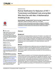
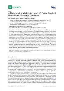
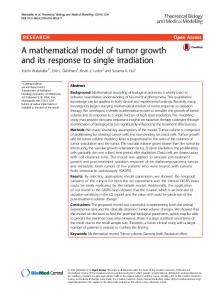
arousal, and a represents the total time of activation elicited by each reinforcer. The cumulative process suggested by Equation 1 is depicted in Figure 1A. The vertical lines represent the impulse Q, which decays exponentially according to ␮. The integral of the decay curves is given by Q␮, justifying the interpretation given to parameter a. Because Equation 1 describes the average arousal between reinforcers, the curve generated by it would lie just below the bold curve that touches the arousal peaks. Applied to within-session responding, the accumulation of arousal may explain the early session increases in response rate (Killeen, 1995). Such warm-up effects failed to be explained by training effects, recovery from handling, and habituation of exploration (McSweeney & Johnson, 1994; McSweeney, Swindell, & Weatherly, 1998; Roll & McSweeney, 1997). According to Killeen (1995), warm-up occurs when successive reinforcers drive the organism to an increasingly high activation state. In support of this hypothesis, it should be noted that within-session responding peaks earlier when reinforcers are scheduled to be presented at high frequency (McSweeney & Hinson, 1992). Besides its utility, Equation 1 is incomplete. It disregards the loss of reinforcer efficacy that inevitably occurs across successive presentations as a result of processes such as satiation and habituation. Those processes are generally claimed to be responsible for the late session decreases in responding observed in many operant

293

sessions (DeMarse, Killeen, & Baker, 1999; Killeen, 1995; McSweeney, 2004). Seeking to incorporate satiety effects in his arousal model, Killeen (1995) postulated that, across an experimental session, a linear decrease in deprivation (d) occurs as a function of time. He also postulated the existence of a motivational drive (h) linked to deprivation in a simple linear or exponential relation. The linear case would be expressed as ht ⫽ ␥dt, were ␥ is a proportionality constant. The exponential case would be expressed as ht ⫽ e␥dt ⫺ ␪, were ␪ represents a minimum threshold that must be exceeded before responding is initiated. Finally, he suggested that the motivational drive h combines multiplicatively with the value (v) of the reinforcer to determine the reinforcer’s specific activation a, so that a ⫽ vht. Consequently, Equation 1 must be rewritten as: ⫺t

៮ ⫽ vh R(1 ⫺ e ␮ ). A t t

(2)

The model entailed in Equation 2 is depicted in Figure 1B and 1C. Panel B describes the accumulation and decay of arousal considering a linear decay of h. Panel C describes the same process, but assuming an exponential decay of h. Again, the curve generated by Equation 2 is not depicted in the figure, but it would follow closely bellow the thick lines that touch arousal peaks.

Figure 1. Models of arousal. The ordinates represent the animal’s arousal level, and the abscissas represent time. The vertical lines illustrate the jolt of arousal elicited by each reinforcer, which decays exponentially as demonstrated by the thin lines. Successive presentation of reinforcers produces an accumulation of effects, resulting in an average level of arousal approximated by the thick line. A presents the seminal model of Killeen et al. (1978), where the jolt of arousal is constant. In B and C, arousal is pushed down by satiation-based drive decay (Killeen, 1995). Drive decays linearly in B and exponentially in C. D represents the model elaborated in the present study. Note that, in D, the thick line does not violate the thin lines of arousal decay.

BITTAR, DEL-CLARO, BITTAR, AND SILVA

294 The Modeling Mistake

Although capable of drawing a bitonic function of arousal along successive reinforcers, Equation 2 presents a modeling mistake. After the peak, the arousal curve is pulled down by the increasingly smaller motivational drive (h). As it can be seen from Panels B and C of Figure 1, the general arousal A assumes a null value when drive h comes to 0. However, because arousal elicited by each reinforcer decays exponentially, and because exponential decay curves never reach 0, the general arousal A could never be completely extinguished. The reason why Equation 2 produces such a distortion is because all the terms in it are multiplied by the motivational drive h. Drive h is a direct function of deprivation d. Therefore, it decays as deprivation does. However, as we can see from Figure 1B and 1C, at some point each new reinforcer will begin to reduce the general arousal, producing some sort of “negative arousal.” This moment is represented in Figure 1 as the point where the thick line (which illustrates the general level of arousal) crosses the thin lines (which illustrate the course of the arousal elicited by each reinforcer). After this point, the vertical lines that illustrate the jolts Q of arousal and that always depart from the remaining arousal from the previous reinforcer would be representing a subtraction of arousal. It could be argued that, after satiation, the reinforcing stimulus becomes aversive, inhibiting instrumental behavior. But this argument would be invalid for two reasons. First, the subtraction of arousal occurs significantly before drive h reaches a null value. Second, in the context of a free-operant session where subjects work to produce reinforcers, after the crossing point they would be working to produce aversive stimuli—if we assume arousal to be related to operant responding, as Killeen (1994) does. Given the problems entailed in Equation 2, we propose a new model of the dynamics of arousal.

␤, Q is attenuated to approximately 36.8% of its initial value. For n ⫽ 0, Q0 ⫽ Q. Considering Equations 4 and 5, at the time a second reinforcer is presented, the arousal level of the subject will be given by: A2 ⫽ A1e

from the first presentation (A1e

A1 ⫽ Q,

(3)

where Q is the jolt of arousal engendered by the reinforcer. The quantity A1 will decay exponentially over time, according to the function ⫺t

At ⫽ A1e ␮ ,

(4)

where ␮ is the exponential time constant. If we assume that satiation decreases the arousing effect of reinforcers, we must consider that, when the next reinforcer is presented, quantity Q will be slightly smaller. If we assume that Q also decays exponentially, then Qn ⫽ Qe

⫺n ␤

,

(5)

where n is the number of reinforcers previously consumed and ␤ is a constant that dictates how fast satiation proceeds. When n ⫽

⫺1 ␤

,

(6)

⫺1

⫺T ␮ )

plus the new jolt attenuated by

a small satiation (Qe ␤ ). Following the same process, arousal at the third presentation will be: A3 ⫽ A2e

⫺T ␮

⫹ Qe

⫺2 ␤

,

(7)

And arousal at the nth reinforcer will be: An ⫽ An⫺1e

⫺T ␮

⫹ Qe

1⫺n ␤

.

(8)

Equation 8 is a recursive function. solving it for n, and assuming A0 ⫽ 0, we can write it as: T

An ⫽

Qe ␮

⫹

1⫺n ␤

n

⫺T

关⫺1 ⫹ e ␤ 共e ␮ 兲n兴 . T

1

(9)

⫺e ␮ ⫹ e ␤ If we want to know arousal A at moment t into session, instead of after a number n of reinforcers, we can assume that reinforcers are presented at an average rate R, which equals 1/T. We can also assume that n ⫽ Rt. Then, At ⫽

To offer a new model of arousal, we first return to Killeen’s model of arousal as originally presented (Killeen et al., 1978). Immediately after the presentation of a reinforcer, the animal’s level of arousal A1 will be given by:

⫹ Qe

where T is the time elapsed since the last reinforcer. Equation 6 simply states that the animal’s arousal at the presentation of the second reinforcer (A2) will be the remaining arousal

1

Fixing the Bug

⫺T ␮

Qe R␮

⫹

1⫺Rt ␤

⫺t

Rt

共⫺1 ⫹ e ␮ ⫹ ␤ 兲 . 1

1

(10)

⫺e R␮ ⫹ e ␤ The arousal model of Equation 10 is illustrated in Figure 1D. The major difference between Equation 10 and Equation 2 is that, here, the only effect of satiation is that the quantity Q (vertical lines in Figure 1) becomes increasingly smaller with successive reinforcers. Eventually, new reinforcers will add almost nothing to the general state of arousal. When this happens, the animal’s arousal will decay respecting the natural decay of the reinforcers previously presented. The thin lines in Figure 1D are not violated. It should also be noted that, even when the animal reaches total satiation, Equation 10 predicts it will continue to respond until all the previously elicited arousal dissipates. The effect of satiation is simply to decrease the arousing effect of each new reinforcer—it cannot affect the general arousal level engendered by the reinforcers presented earlier in the session. This is a very important difference from Equation 2, and may help explain at least one instance of what Morgan (1974) termed “resistance to satiation.” As he noticed, It sometimes happens that an experimenter is careless enough to leave a rat in automated testing apparatus for much longer than the usual session length. When the rat is finally removed, the food cup is often found to be full of reward pellets, that the rat has evidently obtained by lever pressing, but not consumed. (Morgan, 1974, pp. 451– 452)


The lever pressing under satiation is sustained by what is left of the arousal that was previously elicited. The animal continues to respond, but his arousal level is not being augmented anymore. Residual arousal rapidly fades, carrying the response rate along with it. This hypothesis is supported by Myers (1960), who reported that “during the accumulation of pellets . . ., the rats’ response rates decline rapidly until responding ceases entirely.”

A Word on a Controversy Before we proceed to the next step in constructing our model, it is important to clarify that we use the term satiation within a broad definition that includes postingestive factors (e.g., level of sugar in the blood, stomach distension, tissue hydration etc.) as well as preingestive factors (i.e., habituation to the sensory properties of the reinforcer). The relative contribution of post- and preingestive factors to the decrement in responding is still under dispute. While Killeen and his colleagues emphasize the importance of postingestive factors (Killeen, 1995; DeMarse, Killeen, & Baker, 1999), McSweeney and her colleagues have demonstrated that the preingestive factors may overcome the effects of postingestive factors in conditions where these two components of satiation are varied in opposite directions (Aoyama & McSweeney, 2001; McSweeney, 2004). The equations above are silent about this controversy. They simply state that the arousal elicited by each reinforcer (Q) decreases as more reinforcers are presented and consumed. They do not try to answer whether the factors promoting the decay of Q are mainly post- or preingestive.

Constraining Arousal In MPR, arousal is directed by coupling to produce operant responding (Killeen, 1994; Killeen & Bizo, 1998). Operant responding, in its turn, is constrained by time. This point is important: time constrains responding, not arousal. MPR takes arousal as a linear function of reinforcement rate (Killeen & Bizo, 1998; Killeen & Sitomer, 2003). As such, arousal is free to reach unlimitedly high values as the rate of reinforcement increases. Here, we maintain the assumption that organisms behave under constraints. However, we consider that arousal itself is also constrained, because the hypothesis that organisms can be unlimitedly excited seems unreasonable from a biological point of view. To limit the increase of arousal, we may consider it as a variable that varies in the range of 0 to 1. Then, we multiply its value by its distance to the ceiling. In this way, when arousal is low, its growth is not significantly restrained, because the distance to the ceiling is close to 1. As arousal rises, the distance to the ceiling comes close to 0, and growth is heavily restrained. Mathematically, adding this ceiling effect means multiplying Equation 10 by 1 ⫺ A and solving for A, which yields: 1

At ⫽

Qe R␮ 1

⫺Qe R␮

⫹

1 ␤

Rt

⫹

1 ␤

关

⫺t

Rt

共⫺1 ⫹ e ␮ ⫹ ␤ 兲 1

1

共

⫺t

⫹ e ␤ e ␤ ⫹ e R␮ ⫺1 ⫹ Qe ␮

⫹

1 ␤

兲兴

.

(11)

Equation 11 is clearly not as simple as Equation 2, but it is conceptually consistent. It models a process where reinforcers add arousal and satiation subtracts the arousal adding effect of reinforcers, up to a point where it begins to dissipate according to its natural course. Moreover, arousal is presented here as a dimen-

295

sionless variable with range between 0 (no arousal at all) and 1 (maximum arousal supported by the organism’s biology).

From Arousal to Responding Equation 11 describes how arousal accumulates and dissipates in the course of an experimental session, but unless it is placed inside a general model of response rate, it will say much about a hypothetical construct but nothing about objective behavioral data we want to model and predict. Following MPR’s basic assumptions, we now need to consider how coupling directs arousal, producing operant responding (Killeen, 1994; Killeen & Bizo, 1998). To do this, we simple multiply Equation 11 by C, a coupling coefficient that varies between 0 and 1 and represents the degree to which target responses and reinforcers are associated in the subjects’ STM (Killeen, 1994). The product of A and C represents the amount of arousal directed to emission of target responses. Considering a hypothetical situation where the animal is totally aroused (A ⫽ 1), and where there is perfect coupling (C ⫽ 1), we would expect to obtain the maximum response rate attainable. This maximum response rate can be represented as 1/␦, where ␦ is the time required for the emission of a single response. Otherwise, in a situation where directed arousal (AC) is 0.5 we would expect a response rate B ⫽ 0.5/␦. So, as a general law, response rate is given by: AC B⫽ ␦ .

(12)

Equation 12 is the simplest possible formalization of Killeen’s theory of operant behavior (Killeen, 1994). Here, his three principles are present: arousal (A), coupling (C) and time constraints (␦). The relations between these processes and responding are immediately clear: response rate (B) is directly proportional to arousal and coupling, and inversely proportional to the time required to respond. The only reason why Killeen did not come to such a simple solution is because, in his model (Killeen, 1994), arousal is an unconstrained parameter. By assuming A and C as parameters that vary in the range of 0 to 1, we naturally establish a ceiling of 1/␦ to response rate.

Application to Variable Interval (VI) Schedules Killeen (1994) demonstrated that the coupling coefficient for VI schedules is given by: ␳␭B C ⬇ ␭B ⫹ R ,

(13)

where ␭ is the memory-decay rate and ␳ is the coupling constant— related to the proportion of target responses in the overall stream of behavior. For VI schedules, the coupling constant is around 1/3 (Killeen, 1994). Inserting Equation 13 into Equation 12 and solving for B yields: ␳A R B ⫽ ␦ ⫺ ␭.

(14)

The subtrahend plays a significant role only at very high rates of reinforcement, where the reinforcer effects extend back to the prior


296

consummatory response, decreasing coupling and reducing response rates. Omitting it incurs only a small decrease in goodness of fit (Killeen, 1995). For the sake of simplicity, our final model for within-session responding under variable interval schedules will be given by the following: ␳A B⫽ ␦ .

(15)

Next we assess the predictive power of Equation 15 with data from our own laboratory, as well as data from different researchers. But first we refer the reader to Table 1 for a summary of parameters and variables, their interpretations, and dimensions.

Experimental Support Equation 15 postulates that response rate B is a function of ␮, ␳, Q, ␤, ␦, and R. The time constant ␮, which dictates how fast arousal decays, is a variable probably related to the organism’s biology, and therefore should remain constant across a large variety of experimental operations. For most VI schedules ␳ is estimated to remain close to 1/3 (Killeen, 1994). On the other hand, parameters Q, ␤, and ␦ can be indirectly manipulated. We should alter Q and ␤ by changing the reinforcers’ properties, such as its quality and size, as well as the deprivation state. We should alter parameter ␦ through operations that affect response duration. Finally, the rate of reinforcement R can be directly controlled. Now we present empirical data from experiments where within-session response rates were affected by the operations listed above. By fitting Equation 15 to these data we can verify whether its parameters change in the expected directions. In all experiments the model was fitted to data by nonlinear least-squares method. The Excel sheet used for parameter estimates is available to the reader as supplementary material to this article.

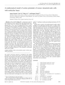
Varying the Rate of Reinforcement (R) In an unpublished experiment from our laboratory (Bittar, 2010), six rats (Group 1) pressed levers under VI schedules of reinforcement with the average interval ranging from 15 to 120 s

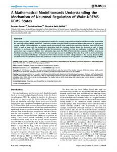
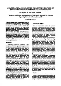
in different conditions. The order of the conditions was randomly determined for each subject, and each condition was maintained in effect during 15 daily sessions. The reinforcers consisted of 0.1 cc of water, and the rats were 20-hr water-deprived at the beginning of each session. Figure 2 shows the within-session response rates during successive 3-min bins, averaged through the last five sessions during which each condition was in effect. Response rates conformed to the patterns typically reported in literature (McSweeney & Hinson, 1992), increasing under VI 60-s and VI 120-s schedules and increasing up to a peak and then decreasing under VI 15-s and VI 30-s schedules. The curves through the data points were drawn by Equation 15, with parameter estimates provided in Table 2. Equation 15 was capable of providing an adequate description of response rates while maintaining parameter estimates at theoretically consistent values. Because the reinforcer stimulus and the deprivation level was the same across different conditions, we set parameter Q at 0.15. Parameter ␮ was set at a constant 6-min value. Parameter ␦ suffered small variations at different VI schedules, floating around 0.5 s per response. Parameter ␤, in its turn, behaved in the most interesting way. It was estimated at 23.6 and 65.2 at VI 15-s and VI 30-s schedules, respectively. Because the reinforcer used in the experiment was a very small amount of water (0.1 cc), it is possible that the minimum satiation provided by each reinforcer dissipated between presentations. At the higher rate of reinforcement provided by the VI 15-s schedule, there was little dissipation, and satiation was faster (smaller value of ␤). At the lower reinforcement rate, however, dissipation of satiation was significant, leading ␤ to a higher value on the VI 30-s schedule. For the VI 60-s and VI 120-s schedules, ␤ took an infinity value, meaning that all satiation dissipated between reinforcements (i.e., deprivation level remained constant throughout the session). Figure 2 also presents data from a different group of five rats (Group 2) responding under a VI 20-s schedule and yet another group of three rats (Group 3) responding under a VI 45-s schedule. Rats on both groups received 30 daily experimental sessions, and the data points represent the response rate averaged over the last five sessions during which each schedule was in effect. Apparatus

Table 1 Parameters and Variables of Equation 15, Their Interpretations, and Dimensions Parameter

Name

B

Response rate

Q

Arousal impulse

R

Rate of reinforcement

␮ ␤ C

Mu Beta Coupling coefficient

␦

Delta

␳

Rho (coupling constant)

Interpretation

Dimension

The number of responses in a time interval divided by the interval’s duration. The jolt of arousal engendered by the first reinforcer in the session. The number of reinforcers presented in a time interval divided by the interval’s duration. The time constant of arousal decay Constant of satiation. The degree to which responses and reinforcers are associated in the animal’s short-term memory. The time required for the emission of a single response. The proportion of target responses in the overall stream of behavior.

1/T 1 1/T T 1 1 T 1


297

Figure 2. Within-session response rates of rats responding on different VI schedules. All circles are from six rats (Group 1), averaged over the last five sessions each condition was in effect. The triangular data points are from three rats (Group 2) on VI 20-s and the diamonds are from five rats (Group 3) on VI 45-s, averaged the same way. The curves were drawn from Equation 15, with parameter estimates given in Table 2.

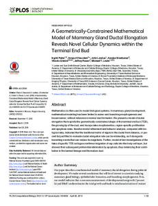
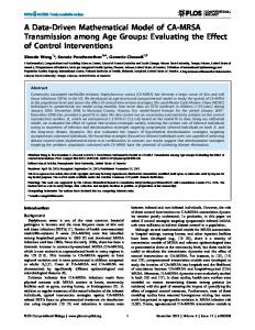
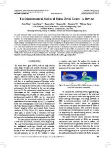
and reinforcer stimuli were the same from the experiment described above. The curve drawn by Equation 15 provided an adequate account of response rates. Estimated parameters are shown in Table 2. Parameters Q and ␮ were settled at their typical values (0.15 and 6-min, respectively). Equation 15 also provided a good fit when applied to McSweeney’s (1992) data. Using lever presses as the target response and 45-mg Noyes pellets as reinforcers, she exposed rats to different VI schedules, presenting her results as proportions (i.e., the number of responses per 5-min component divided by total session responses). We obtained response rate data by multiplying the given proportions by the total session responses and then dividing by 5. Figure 3 demonstrates that Equation 15 provided an accurate description of McSweeney’s results, with the parameter estimates presented in Table 2. Parameters Q and Table 2 Equation 15 Parameter Estimates When Applied to Data From Bittar (2010) and McSweeney (1992) Parameters Study Bittar (2010) – Group 1

Bittar (2010) – Group 2 Bittar (2010) – Group 3 McSweeney (1992)

Condition VI VI VI VI VI VI VI VI VI VI VI

15-s 30-s 60-s 120-s 20-s 45-s 15-s 30-s 60-s 120-s 240-s

␳

␦

Q

␮

␤

1/3 1/3 1/3 1/3 1/3 1/3 1/3 1/3 1/3 1/3 1/3

0.54 0.47 0.45 0.47 0.55 0.74 0.21 0.17 0.17 0.16 0.20

0.15 0.15 0.15 0.15 0.15 0.15 0.15 0.15 0.15 0.15 0.15

6.0 6.0 6.0 6.0 6.0 6.0 6.0 6.0 6.0 6.0 6.0

23.6 65.2 ⬁ ⬁ 21.0 34.2 51.6 67.4 33.1 37.2 32.0

Note. Parameter ␦ is given in seconds, whereas ␮ values are given in minutes.

␮ were set at their standard values. Parameter ␦ floated around 0.18 s per response. Parameter ␤ varied unsystematically, ranging from 32 to 67.4, failing to correlate with the rate of reinforcement. It is probable that parameter ␤ is being forced to correct the simplifications that were adopted when constructing the model. Each simplification is a source of error, which ␤ may be trying to accommodate.

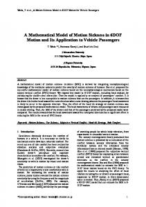
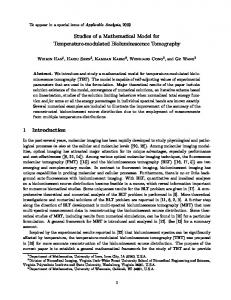
Varying the Response Duration (␦) Melville, Rybiski and Kamrani (1996) trained four rats to press a lever for 45-mg Noyes pellets under a VI 1-min schedule. Then they varied the force required to move the lever from 0.25 N to 1.10 N in different conditions. We fitted Equation 15 to their within-session data, and present the results in Figure 4. The model conformed to the data well, and parameter estimates are presented in Table 3. At all conditions, ␤ took an infinity value, indicating that the deprivation level remained constant along the session. Parameters Q and ␮ were set at their standard values. Finally, only the parameter ␦ changed between experimental conditions. Moreover, the changes were orderly, with ␦ values increasing linearly as the required force increased, as shown in Table 3 (r ⫽ .94). The reader should be reminded that ␦ is the time required to emit a response. Because increasing the force required to operate the lever probably increases the time of the lever-press response, the obtained increases in ␦ shown in Table 3 were expected in advance. The conclusion here is identical to Killeen’s (1994). After analyzing an experiment of Mazur (1982), he concluded that increasing the lever weight results in increases in ␦, while maintaining the arousal level invariant.

Varying the Reinforcer’s Magnitude Cannon and McSweeney (1995) reported an experiment where three pigeons pecked keys on VI 30-s schedules of


298

Figure 3. Within-session response rates of rats responding on different VI schedules in McSweeney’s (1992) experiment. The curves were drawn from Equation 15, with parameter estimates given in Table 2.

reinforcement. The duration of reinforcers (access to mixed grain) varied from 2 s to 20 s in different conditions. They presented their results as the number of responses per 5-min component divided by total session responses, from which we calculated response rate data. The experimental results and the fitted curves from Equation 15 are depicted in Figure 5. Parameter estimates are presented in Table 4. Response duration ␦ was settled at 0.25 s and ␮ at its standard value 6 min. Parameters Q and ␤, on the other hand, were strongly correlated with the reinforcer magnitude, but in opposite directions. As the reinforcer magnitude increased, the jolt of arousal elicited by each reinforcer (Q) increased (r ⫽ .96) while the number of reinforcers needed to produce 63.2% of satiation (␤) decreased (r ⫽ ⫺0.88). In short, we conclude that increasing the reinforcer magnitude affects response rate through a double effect mechanism: Q is increased and ␤ is decreased.

forcer, which decays exponentially throughout the session according to the decay rate ␮.1 Results for both groups, averaged from the last five sessions during which each condition was in effect, are presented in Figure 6, with the curves drawn from the adjusted Equation 15. As can be seen from the parameter estimates presented in Table 5, the most significant changes occurred in the satiation parameter ␤, as could be predicted. This parameter took smaller values (indicating faster satiation) in Group SC than in Group LC. Within groups, satiation proceeded faster at the 5-s hopper access than at the 2-s hopper access condition. When LC subjects responded for 2-s hopper access, no satiation occurred at all (␤ ⫽ ⬁). Parameters Q and ␮ were settled at 0.3 and 6-min, respectively. Parameter ␦ varied around 0.24-s for Group SC and around 0.31-s for Group LC, indicating that SC subjects responded slightly faster.

Alternative Models

Varying the Organism’s Capacity DeMarse, Killeen and Baker (1999) measured the weight of 20 food-deprived pigeons before and after providing 1-hr of access to a food cup. The difference in weight was defined as the pigeons’ eating capacity. The four subjects with greater capacity (M ⫽ 47.5 g) were grouped to form the Group LC while the four subjects with smaller capacity (M ⫽ 19.2 g) formed the Group SC. Then, all pigeons responded under VI 30-s schedules. In different conditions, reinforcers consisted of 2 s or 5 s of access to a hopper containing milo grain. The experimenters also delivered one reinforcer just before the beginning of each session to attenuate warm-up effects (DeMarse et al., 1999). This procedural detail results in the pigeons’ arousal being significantly greater than 0 at the start of the sessions, thus requiring a small adjustment of t Equation 15. To account for their data, we added Qe⫺ ␮ to the arousal model of Equation 11, which is embedded in Equation 15. This term represents the arousal elicited by the presession rein-

Visual inspection of Figures 2 to 6 leaves us with the impression that Equation 15 provides an adequate description of the experiments cited above. However, does Equation 15 describe data better than alternative models? To answer this question we fitted two other models of withinsession responding to the results from the aforementioned experiments. The first model is from Killeen (1995) and the second from McSweeney, Hinson and Cannon (1996). There’s also a linear model from Aoyama (1998), but as Aoyama and t

1

The right thing to do would be to add the initial arousal term (Qe⫺ ␮ ) to Equation 10 and then correct it for ceiling effects to obtain the adjusted model of arousal for this experiment. By adding the term directly to Equation 11 we make it free from ceiling effects, thus allowing arousal to t

exceed 1. However, because adding Qe⫺ ␮ to Equation 10 and then correcting it results in a very complex equation, we choose to privilege simplicity at the cost of a small loss in precision.


299

Figure 4. Within-session response rates of rats, from Melville et al. (1996) experiment. The numbers on the upper-right side of panels represent the force required to move the lever under each condition. The curves were drawn from Equation 15, with parameter estimates given in Table 3.

McSweeney (2001) acknowledged, it cannot account for the bitonic pattern of response rates observed in the behavioral data presented here. Therefore, it was excluded from the analysis below. Before we go on to compare the performance of each of these models, we provide a brief description of these alternative formulations.

M represents the metabolic rate and m represents the size of the reinforcers. Equation 16 simply states that deprivation at time t into session (dt) depends on the initial deprivation level (d0) attenuated by the balance between the resources that have been spent (M) and the resources that have been consumed (mR). To obtain a prediction of operant response rates, Killeen states the following: ៮ kA t

Killeen’s (1995) Model We have seen before that Killeen calculates the within-session arousal level as follows: ⫺t

៮ ⫽ vh R(1 ⫺ e ␮ ). A t t This is Equation 2, and we have already discussed its limitations. The motivational drive ht, in its turn, is given by ht ⫽ ␥dt, where dt ⫽ d␱ ⫹ (M ⫺ mR)t.

(16)

Table 3 Equation 15 Parameter Estimates When Applied to Data From Melville, Rybiski, and Kamrani (1996)

B⫽ ៮ At ⫹ 1

(17)

This equation postulates that response rate is a hyperbolic function of arousal level, scaled by parameter k—the maximum response rate attainable at a specific experimental context, given by C/␦. The entire model has seven parameters (k, v, ␥, d0, M, m, and ␮). Because parameter ␥ is redundant with parameter v, it may be fixed at 1. It is also possible to fix metabolic rate M at 0, assuming that metabolic processes are insignificant in the course of a typical experimental session (Killeen, 1995). Parameter m may be set at 1, leaving deficit d0 to be measured in number of reinforcers. We are finally left with four parameters free to vary: k, v, d0, and ␮.

McSweeney, Hinson, and Cannon’s (1996) Model

Parameters Condition

␳

␦

Q

␮

␤

0.15N 0.25N 0.50N 0.75N 1.10N

1/3 1/3 1/3 1/3 1/3

0.52 0.44 0.56 0.72 0.96

0.15 0.15 0.15 0.15 0.15

6.0 6.0 6.0 6.0 6.0

⬁ ⬁ ⬁ ⬁ ⬁


McSweeney et al. (1996) also provided a model of withinsession operant responding. After examining the fit of several functions to within-session responding data, they arrived at a three parameter equation given by the following: b c P ⫽ eaT ⫺ c ⫹ T .

(18)

where P is the proportion of the total-session responses that occur during successive time bins, and a, b and c are free


300

Figure 5. Within-session response rates of pigeons responding for reinforcers with varied duration between conditions. The curves were drawn from Equation 15, with parameter estimates given in Table 4. The data are from Cannon & McSweeney (1995).

parameters. The first term promotes an exponential decay of response rate attributed to habituation. The second term promotes a hyperbolic increase of response rate attributed to sensitization. These two processes combine to draw a bitonic pattern of response rate along the course of an experimental session. Contrary to Equation 15 and to Killeen’s (1995) model, Equation 18 is an empirical model. Therefore, its parameters have no theoretical meaning.

Comparing the Fits We used the least-squares method to fit Equation 17 (Killeen, 1995) and Equation 18 (McSweeney et al., 1996) to data from all the experiments mentioned above. Then we compared the relative goodness of fit of these models and Equation 15 using the bias-corrected Akaike Information Criteria (AICc), which is preferred over traditional AIC when working with small sample sizes (Spiess, & Neumeyer, 2010). The Akaike weights for all models for all conditions of all experiments are presented in Table 6. At each condition these weights can be interpreted as

the probability of a specific model being the best model among its competitors (therefore, Akaike weights in a row must always add up to 1). Equation 15 performed better than the alternative models in 19 of 25 comparisons (76%). McSweeney’s model performed better in 5 comparisons (20%) and Killeen’s model in one (4%). Besides often providing a better fit to data, Equation 15 also provides a better fit to theory. While McSweeney’s model is admittedly empirical, Killeen’s model has some flaws in its construction. The model outlined here, on the other hand, is solidly grounded in MPR’s core principles (Killeen, 1994). As a consequence, its parameters have clear theoretical meanings, assuming values that are immediately interpretable and easy to compare and understand.

Table 4 Equation 15 Parameter Estimates When Applied to Data From Cannon & McSweeney (1995) Parameters Condition

␳

␦

Q

␮

␤

2-s 5-s 8-s 15-s 20-s

1/3 1/3 1/3 1/3 1/3

0.25 0.25 0.25 0.25 0.25

0.03 0.05 0.04 0.09 0.10

6.0 6.0 6.0 6.0 6.0

53.7 63.7 33.9 10.7 16.9


Figure 6. Within-session response rates of large capacity (LC) and small capacity (SC) rats responding for reinforcers with varied duration between conditions. The curves were drawn from Equation 15, with parameter estimates given in Table 5. The data are from DeMarse, Killeen, & Baker (1999).


Table 5 Equation 15 Parameter Estimates When Applied to Data From DeMarse, Killeen, and Baker (1999) Parameters Condition Group Group Group Group

SC 2-s SC 5-s LC 2-s LC 5-s

␳

␦

Q

␮

␤

1/3 1/3 1/3 1/3

0.23 0.25 0.29 0.33

0.3 0.3 0.3 0.3

6.0 6.0 6.0 6.0

130.1 21.9 ⬁ 63.4


Conclusion In the present study, we relied on simple assumptions to derive a formal model of arousal dynamics. The assumptions were as follows: (a) reinforcers arouse organisms, (b) the arousal decays over time, (c) the arousal accumulates, (d) reinforcers lose their arousal effect trough successive presentations, and (e) there is a limit to the degree an organism can be aroused. The first three assumptions were also present in Killeen’s (1995) model of arousal dynamics. However, the process by which successive reinforcer presentations affect arousal was not clearly devised, leading his model to a modeling mistake. Killeen’s arousal model also lacks a ceiling. Later, additional assumptions were made to allow the prediction of

301

response rates. They were as follows: (f) a fraction C of an organism’s arousal is directed to emission of target responses, and (g) time constrains responding. These two principles are not new, and they are at the core of MPR (Killeen, 1994). These seven assumptions were formally elaborated, resulting in an equation that describes response rate as a function of six variables: (1) the arousal impulse Q, (2) the time constant of arousal decay ␮, (3) the constant of satiation ␤, (4) the coupling coefficient C, (5) the response duration ␦, and (6) the rate of reinforcement R. Application of the model to experimental data from different laboratories demonstrated its generality and comparison with alternative models attested to its adequacy. The model provided a good description of the responding of rats and pigeons working for different reinforcers under different experimental conditions. The parameters of the equation changed in the predicted ways when they were fitted to behavioral data. The arousal impulse Q correlated with the reinforcers’ magnitude. The constant of satiation ␤ correlated with the reinforcer magnitude, with the organism’s capacity, and sometimes with the rate of reinforcement. The response duration ␦ correlated with the force required to respond. The time constant of arousal decay ␮ remained invariant across experimental manipulations, always settled at 6-min. This value of ␮ was also estimated by Killeen et al. (1978), who measured how fast pigeons’ activity decays after a single feeding. Besides providing a consistent model of arousal dynamics, the present study demonstrates the utility of within-session

Table 6 Akaike Weights for Equation 15, Equation 17 (Killeen, 1995), and Equation 18 (McSweeney et al., 1996) for All Conditions of All Experiments Mentioned in the Present Study Model Study Bittar (2010) – Group 1

Bittar (2010) – Group 2 Bittar (2010) – Group 3 McSweeney (1992)

Melville, Rybiski, & Kamrani (1996)

Cannon & McSweeney (1995)

DeMarse, Killeen & Baker (1999)

Note.

Condition VI 15-s VI 30-s VI 60-s VI 120-s VI 20-s VI 45-s VI 15-s VI 30-s VI 60-s VI 120-s VI 240-s 0.15 N 0.25 N 0.50 N 0.85 N 1.10 N 2-s 5-s 8-s 15-s 20-s SC 2-s SC 5-s LC 2-s LC 5-s

Eq. 15 *

0.9885 0.9743 * 0.8121 * 0.9820 0.2273 * 0.9878 * 0.9581 0.1209 * 0.9033 * 0.8422 * 0.7221 0.0773 * 0.8125 * 0.7721 0.0056 0.4700 * 0.8591 * 0.7082 0.2865 * 0.9998 * 0.6917 * 0.9256 * 0.9940 * 0.9488 * 0.9394 *

McSweeney et al. (1996)

Killeen (1995)

0.0106 0.0255 0.1877 0.0178 0.0125 0.0121 0.0418 * 0.8663 0.0899 0.1514 0.2687 * 0.9215 0.1775 0.2230 * 0.9867 * 0.5134 0.1042 0.0191 * 0.7134 0.0002 0.3083 0.0722 0.0060 0.0512 0.0572

0.0009 0.0002 0.0002 0.0002 * 0.7601 0.0001 0.0002 0.0128 0.0068 0.0064 0.0092 0.0013 0.0100 0.0049 0.0077 0.0165 0.0367 0.2727 0.0001 0.0000 0.0000 0.0022 0.0000 0.0000 0.0034

The asterisks indicate the higher Akaike weight for each comparison.


302

operant responding data. Because schedules of reinforcement are generally held constant throughout the session, observed variations in response rate must be primarily attributed to changes in processes such as arousal, satiation, and habituation. As a consequence, within-session data provide a valuable means to clarify the relation between performance and important motivational variables. Finally we demonstrated that, by representing arousal as a parameter in the range of 0 to 1, we can formalize MPR (Killeen, 1994) in the simplest and most intuitive form of Equation 12.

References Aoyama, K., & McSweeney, F. K. (2001). Habituation may contribute to within-session decreases in responding under high-rate schedules of reinforcement. Animal Learning & Behavior, 29, 79 –91. doi:10.3758/ BF03192817 Aoyama, K. (1998). Within-session response rate in rats decreases as a function of amount eaten. Physiology & Behavior, 64, 765–769. doi:10 .1016/S0031-9384(98)00118-8 Bittar, E. G. (2010). Within-session responding under several variable interval schedules of reinforcement. Unpublished manuscript. Cannon, C. B., & McSweeney, F. K. (1995). Within-session changes in responding when rate and duration of reinforcement vary. Behavioural Processes, 34, 285–292. doi:10.1016/0376-6357(95)00009-J DeMarse, T. B., Killeen, P. R., & Baker, D. (1999). Satiation, capacity, and within-session responding. Journal of the Experimental Analysis of Behavior, 72, 407– 423. doi:10.1901/jeab.1999.72-407 Falk, J. L. (1961). Production of polydipsia in normal rats by an intermittent food schedule. Science, 133, 195–196. doi:10.1126/science.133 .3447.195 Falk, J. L. (1972). The nature and determinants of adjunctive behavior. R. M. Gilbert & J. D. Keehn (Eds.), Schedule effects: Drugs, drinking, and aggression. Toronto, Canada: University of Toronto Press. Killeen, P. R., & Bizo, L. A. (1998). The mechanics of reinforcement. Psychonomic Bulletin & Review, 5, 221–238. doi:10.3758/BF03212945 Killeen, P. R., Hanson, S. J., & Osborne, S. R. (1978). Arousal: Its genesis and manifestation as response rate. Psychological Review, 85, 571–581. doi:10.1037/0033-295X.85.6.571 Killeen, P. R., & Sitomer, M. T. (2003). MPR. Behavioural Processes, 62, 49 – 64. doi:10.1016/S0376-6357(03)00017-2 Killeen, P. R. (1994). Mathematical principles of reinforcement. Behavioral and Brain Sciences, 17, 105–172. doi:10.1017/S0140525 X00033628 Killeen, P. R. (1995). Economics, ecologics, and mechanics: The dynamics of responding under conditions of varying motivation. Journal of the Experimental Analysis of Behavior, 64, 405– 431. doi:10.1901/jeab.1995 .64-405 Mazur, J. E. (1982). A molecular approach to ratio schedule performance. M. L. Commons, R. J. Herrnstein & H. Rachlin (Eds.), Quantitative analyses of behavior. Vol. 2: Matching and maximizing accounts. Pensacola, FL: Ballinger.

McSweeney, F. K., Hatfield, J., & Allen, T. M. (1990). Within-session responding as a function of post-session feedings. Behavioural Processes, 22, 177–186. doi:10.1016/0376-6357(91)90092-E McSweeney, F. K., Hinson, J. M., & Cannon, C. B. (1996). Sensitizationhabituation may occur during operant conditioning. Psychological Bulletin, 120, 256 –271. doi:10.1037/0033-2909.120.2.256 McSweeney, F. K., & Hinson, J. M. (1992). Patterns of responding within sessions. Journal of the Experimental Analysis of Behavior, 58, 19 –36. doi:10.1901/jeab.1992.58-19 McSweeney, F. K., & Johnson, K. S. (1994). The effect of time between sessions on within-session patterns of responding. Behavioural Processes, 31, 207–217. doi:10.1016/0376-6357(94)90007-8 McSweeney, F. K., Roll, J. M., & Weatherly, J. N. (1994). Within-session changes in responding during several simple schedules. Journal of the Experimental Analysis of Behavior, 62, 109 –132. doi:10.1901/jeab.1994 .62-109 McSweeney, F. K., Swindell, S., & Weatherly, J. N. (1998). Exposure to context may contribute to within-session changes in responding. Behavioural Processes, 43, 315–328. doi:10.1016/S0376-6357(98)00026-6 McSweeney, F. K., Weatherly, J. N., & Swindell, S. (1995b). Withinsession changes in key and lever pressing for water during several multiple variable-interval schedules. Journal of the Experimental Analysis of Behavior, 64, 75–94. doi:10.1901/jeab.1995.64-75 McSweeney, F. K. (1992). Rate of reinforcement and session duration as determinants of within-session patterns of responding. Animal Learning & Behavior, 20, 160 –169. doi:10.3758/BF03200413 McSweeney, F. K. (2004). Dynamic changes in reinforcer effectiveness: Satiation and habituation have different implications for theory and practice. The Behavior Analyst, 27, 177–188. Melville, C. L., Rybiski, L. R., & Kamrani, B. (1996). Within-session responding as a function of force required for lever press. Behavioural Processes, 37, 217–224. doi:10.1016/0376-6357(96)00008-3 Morgan, M. J. (1974). Resistance to satiation. Animal Behaviour, 22, 449 – 466. doi:10.1016/S0003-3472(74)80044-8 Myers, R. D. (1960). Spontaneous hoarding during operant conditioning. Journal of the Experimental Analysis of Behavior, 3, 154. Roll, J. M., & McSweeney, F. K. (1997). Within-session changes in operant responding when gerbils (Meriones unguiculatus) serve as subjects. Current Psychology: A Journal for Diverse Perspectives on Diverse Psychological Issues, 15, 340 –345. doi:10.1007/s12144-9971011-2 Spiess, A. N., & Neumeyer, N. (2010). An evaluation of R2 as an inadequate measure for nonlinear models in pharmacological and biochemical research: A Monte Carlo approach. BMC pharmacology, 10, 6. doi:10 .1186/1471-2210-10-6 Wallace, M. & Singer, G. (1976). Schedule induced behavior: A review of its generality, determinants, and pharmacological data. Pharmacology, Biochemistry and Behavior, 5, 483– 490. doi:10.1016/00913057(76)90114-3

Received December 12, 2011 Revision received April 10, 2012 Accepted May 3, 2012 䡲