Towards a Mental Probability Logic - CiteSeerX

Towards a Mental Probability Logic∗ Pfeifer, N. & Kleiter, G. D.† Fachbereich Psychologie, Universit¨ at Salzburg (Austria)

(Version October 30, 2007)

Abstract We propose probability logic as an appropriate standard of reference for evaluating human inferences. Probability logical accounts of nonmonotonic reasoning with system p, and conditional syllogisms (modus ponens, etc.) are explored. Furthermore, we present categorical syllogisms with intermediate quantifiers, like the “most . . . ” quantifier. While most of the paper is theoretical and intended to stimulate psychological studies, we summarize our empirical studies on human nonmonotonic reasoning.

1

Introduction

This journal issue is devoted to human thinking and reasoning with inconsistency. The present paper, though, is written within an approach that is deeply obliged to subjective probability and to a property that is at the very core of subjective probability theory, namely coherence. With respect to the present paper the expectations of the reader may mislead him or her. We will neither treat an incoherent approach to human inference, nor shall we try to explain incoherent inferences. On the contrary, we will argue that the traditional gold standard of human reasoning, namely classical logic, is too strong to be an appropriate standard for everyday reasoning and that weaker systems such as subjective probability and nonmonotonic reasoning are more appropriate standards with which human inference should be ∗

A previous version of this paper has been published as: Pfeifer, N. & Kleiter, G. D. (2005). Towards a mental probability

logic. Psychologica Belgica, 45 (1), p. 71-99. † Supported by the KONTAKT 2004/19 Project, Austrian-Czech exchange program.

1

evaluated. Thus, we will try to re-concile the reader’s expectations and the content of our contribution by relaxing the normative standards by which human inference is evaluated. Why do we consider probability theory to be relevant to human inference? In particular, why do we consider probability theory to be relevant even in tasks that apparently do not to involve probabilities or do not explicitly mention uncertainties? Let us anticipate just three main reasons, the details of which will be given in the sequel: 1. Monotonicity is the central property of the classical logical consequence relation: the set of conclusions can only increase but not decrease by adding further premises. This means conclusions cannot be retracted in the light of new evidence. Since retracting conclusions in the light of new evidence makes psychological sense, it is implausible to assume classical logic as the normative standard of reference for evaluating human reasoning—on a priori grounds. 2. Many inferences in propositional logic involve conditionals of the form if A then B in their premises. Typical valid examples are the modus ponens and the modus tollens, which are opposed to the invalid denying the antecedent and affirming the consequent. We do not think that the ordinary conditional appearing in everyday life is the material implication of classical logic. Rather, people evaluate the probability of B given, hypothetically, A, as suggested by Ramsey 80 years ago and recently in psychology (Evans & Over, 2004). In everyday contexts it seems to be more plausible to interpret conditionals not by material implications, but by much weaker conditional probabilities. 3. Likewise, the universal (“all . . . ”) and existential (“at least one . . . ”) quantifiers of predicate calculus are psychologically too strict. For the well-known syllogisms intermediate quantifiers were proposed in the literature. As nonmonotonic conditionals, they allow for exceptions and admit a probabilistic interpretation. We propose a combination of logic and probability, namely probability logic, as an adequate normative standard of reference.

1.1

Logic

There is a tradition of nearly one-hundred years of experiments on deductive reasoning and a tradition of nearly fifty years of experiments on judgment under uncertainty. Usually, the experimental tasks and the normative theories of deductive reasoning are closely related to logic, while the experimental tasks and the normative theories of uncertain reasoning are closely related to probability theory. For 2

many years both traditions were clearly separated. Only recently has the psychology of deductive and of probabilistic reasoning begun to merge (Chater & Oaksford, 1999, 2004; Evans et al., 2003; Evans & Over, 2004; Oberauer & Wilhelm, 2003; Over & Evans, 2003; Pfeifer & Kleiter, 2003, 2005a, 2005b; Politzer & Bourmaud, 2002). Today probabilistic principles are applied to model deductive reasoning and, likewise, principles originally developed in the tradition of deductive reasoning are extended to cover uncertain reasoning. Chater & Oaksford (2004) were among the first who proposed a probabilistic account of Wason’s Selection Task (Oaksford & Chater, 1998), conditional syllogisms (Oaksford, Chater, & Larkin, 2000), and categorical syllogisms (Chater & Oaksford, 1999). Mental probability logic (as proposed in the present paper) is a framework to investigate human reasoning experimentally and theoretically. It is in many respects closely related the Probability Heuristics Model (Chater & Oaksford, 2004). Probability logic, though, seems to be a more systematic approach. It combines explicitly logic and probability. Logic is the language of inferences under certainty and probability logic is the language of inferences under uncertainty. We are challenging the question of the choice of an appropriate normative standard of reference for modeling and evaluating human reasoning. Why is classical logic not an adequate standard of reference for evaluating human reasoning? We discuss two crucial sets of problems: one concerns the material implication, A → B. The other, which is more general, concerns the monotonicity property of the classical logical consequence relation. Problem 1: Material Implication

The problem with the material implication is that it is too strict

for modeling human inference. It neither allows exceptions nor does it allow uncertainty. Furthermore, it is well known that the material implication leads to valid but highly implausible inference rules (Adams, 1975, 1998). Consider the following list:

¬A

∴

A→B

B

∴

A→B

¬A

∴

A → ¬A

¬(A → B)

∴

A

C→B

∴

C∧A→B

3

Why are these inference rules implausible (we omit the proof of their logical validity)? Hardly anyone would infer that “if The sun is shining, then It is raining”, (A → B), from “it is not the case that: The sun is shining”, (¬A). Likewise, “if The sun is shining, then It is raining”, (A → B), will not be plausibly inferred from “It is raining”, (B). Subjects will not infer “if The sun is shining, then it is not the case, that: The sun is shining”, (A → ¬A), from “The sun is shining”, (A). Should we really conclude that “The sun is shining”, (A), from “it is not the case that: if The sun is shining, then It is raining”, (¬(A → B))? Finally, it is also very implausible to conclude that “if The aeroplane is flying at time t and The aeroplane is hit by a missile at time t, then All guests at the aeroplane are rather safe at time t”, (C ∧ A → B), from the conditional “if The aeroplane is flying at time t, then All guests at the aeroplane are rather save at time t”, (C → B). Such implausible, though logically valid, inferences which are consequences of the material implication led many authors to rethink the interpretation of everyday reasoning with expressions of the form “if A, then B”. One attempt to avoid such problems is to combine logic and probability. Let us now turn to the second psychologically problematic property of classical logic. Problem 2: Monotonicity

Monotonicity is the central property of the classical logical consequence

relation: the set of conclusions can only increase but not decrease by adding further premises. Conclusions cannot be retracted in the light of new evidence. A framework that does not have this problematic property is nonmonotonic reasoning. Nonmonotonic reasoning allows one—contrary to classical (monotone) logics—to withdraw conclusions in the light of new evidence. The classical example is the “Tweety” argument: Assume as premises that birds can fly, and that Tweety is a bird. Therefore, you conclude that Tweety can fly. As soon as you learn that Tweety is a penguin you will withdraw the conclusion that Tweety can fly. Classical logic is monotone in the sense that adding arbitrary premises to arguments monotonically increases the set of conclusions, i.e. conclusions cannot be withdrawn.1 Since withdrawing conclusions in the light of new evidence is natural in everyday reasoning, classical logic appears to be an a priori implausible standard of reference for human reasoning. 1

To prove the monotony of classical logic, assume that A |= B (i.e., A logically entails B). Let α be an arbitrary model

such that |=α A ∧ C. Therefore |=α A. Since our assumption claims that for all models β: if |=β A, then |=β B (that is A |= B), we get by instantiation of α for β: if |=α A, then |=α B, which logically implies together with |=α A: |=α B. It is now proven that for an arbitrary α: if |=α A ∧ C, then |=α B. Therefore A ∧ C |= B, and this completes the proof that A |= B logically implies A ∧ C |= B.

4

Nonmonotonic reasoning is often claimed to mimic human common sense reasoning. Compared with the long tradition of psychological experiments on classical logics and syllogistics (Rips, 2002, 1994; Johnson-Laird, 1999; Johnson-Laird & Byrne, 1991; Bacon et al., 2003; Newstead, 2003; Morley et al., 2004), only a few studies, though, have investigated nonmonotonic reasoning empirically (Benferhat et al., in press; Da Silva Neves et al., 2002; Ford & Billington, 2000; Ford, in press, 2004; Pfeifer, 2002; Pfeifer & Kleiter, 2003, 2005a; Pelletier & Elio, 2003; Schurz, in press).

1.2

Subjective Probability

There are several different approaches to probability.2 From a psychological perspective it is highly plausible to compare human uncertain reasoning with an approach that is “close” or “affine” to psychology. This is, no doubt, the subjective approach. Since modern subjective probability theory may not be so well known, we summarize some major points that are relevant to psychology. There are a number of deviations from textbook treatments of probability theory that have important implications for psychological research. For details the reader is referred to Coletti & Scozzafava (2002). Subjective probabilities are coherent descriptions of partial knowledge states. Subjective probabilities are not (objective) physical properties of the external world. Thus, the primary psychological question is how humans process partial knowledge. The question is not how human subjects understand probabilities, where probabilities are conceived as physical properties of the external world. This would lead to what we call the “psychophysics metaphor”, comparing, e.g., actual relative frequencies with estimated relative frequency (Kleiter et al., 2002). The subjective approach conceives probabilities as a mapping of incomplete knowledge states to degrees of beliefs, coherently expressed by numbers between 0 and 1. Relative frequencies and proportions can be important in reducing uncertainty and updating degrees of belief, but they should not be confused with probabilities. Of course, whether human judgments and inferences actually are coherent or not, in which conditions, and to what degree, are empirical questions. The “carrier entities” to which probabilities are assigned are propositions or events. Propositions are 2

One can distinguish objective (e.g., classical probability, Laplace etc.; probabilities as relative frequencies in the long run,

von Mises) from subjective (e.g., probabilities as degrees of belief, de Finetti (1974), Ramsey, Savage, Coletti & Scozzafava (2002)), and mixtures of objective and subjective accounts (Good, Halpern et al. (1996)). Furthermore, there are several different proposals about the entities to which probability-values are assigned: sets (e.g., Kolmogorov (1933)), events, propositions (e.g., early Carnap), etc. Most authors start by introducing absolute (one-place) probabilities, P (·), and then define conditional (two-place) probabilities, P (·|·). Others (originally Popper (1994) and R´enyi (1955), later Coletti, Gilio, or Scozzafava start by giving the axioms of P (·|·).

5

either “true” or “false” and the truth values follow the usual rules of Boolean algebra. Truth values in the context of conditional events, though, behave fundamentally different from truth values of non-conditional events. Let Ai and Bi be two propositions and Ai |Bi denote the conditional event Ai given Bi . We denote by |Ai |, |Bi |, and |Ai |Bi | the indicator function of the respective propositions, mapping the truth values of the propositions into numbers, typically 1 (“true”) and 0 (“false”). What are the truth values of a conditional event Ai |Bi ? If Bi is true the answer is straightforward    1 : if Ai = 1 and Bi = 1, |Ai |Bi | =   0 : if A = 0 and B = 1. i i

What is the truth value of Ai |Bi if Bi is false? For this case de Finetti proposed a third truth value “undetermined”, denoted by ∗ ,    ∗ :

|Ai |Bi | = 

 ∗ :

if

Ai = 1 and

Bi = 0,

if

Ai = 0 and

Bi = 0.

An obvious consequence is that conditioning cannot be treated by the usual operators of negation, conjunction, and disjunction. There is no logical operator of conditioning. “Logic lacks a conditioning operator corresponding to conditional probability” (Goodman et al., 1991). This is a fundamental property (Lewis triviality result), that distinguishes conditioning from material implication. De Finetti’s proposal was improved by Gilio (2002) and Coletti & Scozzafava (2002). If the conditioning proposition is false, then the indicator value of Ai |Bi is the value of the conditional probability P (Ai |Bi ) :

|Ai |Bi | =

      

1 :

if

Ai = 1

and Bi = 1,

0 :       P (Ai |Bi ) :

if

Ai = 0

and Bi = 1,

if

Bi = 0.

This proposal makes it possible to determine upper and lower probabilities by elegant and general methods of linear algebra. If the conditioning event turns out to be false we do not learn anything about the probability of Ai . It remains the same as if we would know nothing about Bi . Expressed in terms of bets, the bet is called off and the prize of the bet is payed back. A similar proposal was made by Ramsey in 1929:

6

“If two people are arguing “If p will q?” and are both in doubt as to p, they are adding p hypothetically to their stock of knowledge and arguing on that basis about q; [. . . ] We can say they are fixing their degrees of belief in q given p. If p turns out false, these degrees of belief are rendered void.” (Ramsey, 1994, Footnote, p. 155) Subjective probability theory provides a tailor-made framework that perfectly fits the structure of logical inference problems. We consider a family of arbitrary conditional events F = (A1 |B1 , . . . , An |Bn ), an associated probability assessment Pn = (p1 , . . . , pn ), and one further conditional event An+1 |Bn+1 . In the context of probability logic the set F corresponds to the premises, Pn to the probabilities of the premises, and An+1 |Bn+1 to the conclusion. In both verity logic and in probability logic we consider a set of premises and a conclusion. In verity logic the truth values of the premises are given and the inference problem consists in finding the truth value of the conclusion. In probability logic the probabilities of the premises are given and the inference problem consists in finding the probability of the conclusion. The set F corresponds to the premises, Pn to the probabilities of the premises, and An+1 |Bn+1 to the conclusion. The problem is solved when P (An+1 |Bn+1 ) is determined. If the probabilities of the premises are precise (point probabilities), then the probability of the conclusion is obtained by the Fundamental Theorem of de Finetti. If the probabilities of the premises are imprecise (upper and lower probabilities, intervals), then the probability of the conclusion is obtained by theorems based on generalized coherence (g-coherence, Biazzo et al. (2002)). F need not be an algebra. That is an important difference to the standard approach. When considering conditional events we need not suppose to know the probability of any other events not occurring in the premises. In the case of a probabilistic modus ponens, e.g., only P (A|B) and P (B) are supposed to be known, not the probability of any of the elementary constituents like P (A ∧ B). Moreover P (A|B) and P (B) need not be given in the form of point probabilities. They may be imprecise and may be specified by upper and lower probabilities only (or may even be given in the form of intervals of a second order probability distribution). If we would suppose to know, say, P (A ∧ B), we would actually introduce an additional premise. This would be analog, say, to supposing that A ∧ B is true in a modus ponens in verity logic. We would not need any of the premises of the modus ponens to infer the truth of the conclusion. Likewise, assuming stochastic independence of A and B would correspond to an additional premise.

7

The standard approach to probability theory is characterized by the syntactical apparatus of measure theory (algebras, σ-algebras, Kolmogorov tradition) and the semantical interpretation of relative frequencies in the long run (von Mises tradition). In the subjective approach probability is syntactically processed as a linear operator and semantically interpreted as a coherent degree of belief. Conceiving uncertainty in the way subjective probability theory does poses two questions for the psychology of uncertain reasoning: First the syntactical question, do human subjects have an intuitive understanding of the linear constraints that govern probability theory and probability logic? And second, how do they process their own degrees of belief and those of other people? There are two equivalent ways how to introduce coherence. First, by the well-known Dutch book condition: A probability assessment P = (p1 , . . . , pn ) is coherent if it avoids sure loss. Second, by the relationship to the standard approach: An assessment is coherent if the family F can be expanded to an algebra A such that P satisfies the Kolmogorov axioms for finite sets of events (Coletti & Scozzafava, 2002). Coherence can be generalized to situations in which only lower and upper probabilities are given (Biazzo & Gilio, 1999).

1.3

Probability Logic

Probability logic combines probability and logic. We distinguish verity logic (i.e., logic in the classical sense) and probability logic (Hailperin, 1996). Verity logic is concerned with the truth or the falsity of propositions and with deductive inferences. Classical argument forms like the modus ponens or the modus tollens belong to verity logic. Probability logic is an extension of verity logic that adds probabilistic valuations to the propositions involved in the inferences. It investigates the same argument forms as verity logic, but propagates of probabilities from the premises to the conclusions instead of binary truth values. The argument forms that are best known are syllogisms. There are two kinds of syllogisms: conditional and categorical syllogisms. Conditional syllogisms only rely on propositional calculus, categorical syllogisms require quantifiers. Conditional syllogisms are part of the classical repertoire of verity logic. Well known are the valid modus ponens and modus tollens, and the invalid denying the antecedent and affirming the consequent. The verity versions of conditional syllogisms were extensively investigated empirically (Evans, 1977; Kern et al., 1983; Marcus & Rips, 1979; Markovits, 1988; Rumain et al., 1983; Taplin, 1971) in experiments on deductive reasoning. For discussions see Evans et al. (1993), Rips (1994), Braine 8

& O’Brien (1998). Each of these verity versions has a parallel form in probability logic. Recently psychologists have used probabilistic models to explain deductive reasoning (Chater & Oaksford, 2004). Examples are Wason’s Selection Task (Oaksford & Chater, 1994), matching or set size effects (Yama, 2001; Evans, 2002; Oaksford, 2002), the suppression effect of the modus ponens (Bonnefon & Hilton, 2002), categorical syllogisms (Chater & Oaksford, 1999), and the expertise of a speaker of the premises (Stevenson & Over, 2001). The Probability Heuristics Model (Chater & Oaksford, 1999, 2004) is of course related to our approach, but they are clearly not equivalent. One difference is that often in these experiments the probabilities are not made explicit to the subjects but are only used as parameters in the computational models. A second difference is that the models are not really using probability logic. Four examples of probability logical inferences are given below in Section 3. Usually logical operators are interpreted by a verity function (or valuation function) V that assigns a truth value v ∈ {0, 1} to a (formalized) proposition. Let A and B be arbitrary (atomic or compound) propositions. Then the verity function V is defined as follows (adapted from Hailperin (1996, p. 23f)): V (A)

∈

{0, 1}

V (¬A) =def. 1 − V (A) V (A ∧ B) =def. min(V (A), V (B)) V (A ∨ B) =def. max(V (A), V (B)) V (A → B) =def. V (¬A ∨ B) where “1” and “0” can be interpreted as the truth-values “true” and “false”, respectively. We write arguments in the form of inference rules. The validity of an inference rule is defined analogously to the validity of an argument: an inference rule is valid iff it is impossible to infer a false conclusion from premises that are assumed to be true. The general form of an inference rule is:

P1 , P2 , . . . , Pn ∴ C , where the literal “P1 , P2 , . . . , Pn ” indicates the elements of the premise set (where n is the number of the premises, n ≥ 0, n ∈ N). The premise set can be empty.3 “ ∴ ” is an indicator of the conclusion set. C stands for the conclusion set (there are of course infinitely many conclusions). An example of an inference rule is the following: 3

Logically true propositions, e.g., can always be inferred from the empty premise set.

9

A, B ∴ A∧B , which is read: If A is a premise and if B is a premise, then infer A ∧ B as the conclusion. This is a mere syntactical definition of an inference rule, since no reference to truth values or to any meaning is made. A semantical definition of an inference rule is given in terms of the verity function V : For any verity function V

V (P1 ) ∈ α1 , V (P2 ) ∈ α2 , . . . , V (Pn ) ∈ αn ∴ V (C) ∈ β , where α1 , α2 , . . . , αn , and β are elements of {0, 1}. A natural way of extending inference rules of propositional logic to inference rules of propositional probability logic can be defined as follows: For any probability function P P (P1 ) ∈ α1 , P (P2 ) ∈ α2 , . . . , P (Pn ) ∈ αn ∴ P (C) ∈ β , where α1 , α2 , . . . , αn , and β are real-valued intervals in [0, 1]. The analogy of this definition to the definition of the inference rule in terms of the verity function V is apparent: P replaces V and the truth-value set {0, 1} is extended to the unit interval [0, 1], such that 0 ≤ x∗ ≤ x∗ ≤ 1, where x∗ is called the lower and x∗ the upper bound of the probability interval αi (or β). In case of x∗ = x∗ we also say that αi (or β) is a point probability value. Examples of reasoning with interval-valued and imprecise probabilities are given in the subsequent sections. The next section gives a summary of some of our empirical studies on nonmonotonic reasoning.

2

Nonmonotonic Reasoning—System P

Among various formal systems of nonmonotonic reasoning4 , system p (Adams, 1975; Kraus et al., 1990; Gilio, 2002) has been broadly accepted by the nonmonotonic reasoning community and has gained con4

Default reasoning (Reiter, 1980; Poole, 1980), Autoepistemic (nonmonotonic reasoning) logic (McDermott & Doyle,

1980; Moore, 1985; Konolige, 1994), Circumscription (McCarthy, 1980; Lifschitz, 1994), Defeasible reasoning (Pollock, 1994; Nute, 1994), Default inheritance reasoning (Touretzky, 1986), Possibility theory (Dubois & Prade, 1988; Dubois et al., 1994), and Conditional and preferential entailment: conditional logic-based (Delgrande, 1988; Schurz, 1998), preferential model -based (Kraus, Lehmann, & Magidor, 1990; Lehmann & Magidor, 1992), expectation-ordering-based (G¨ ardenfors & Makinson, 1994), and probabilistic entailment-based approaches (Gilio, 2002; Adams, 1975; Pearl, 1988, 1990; Schurz, 1998), just to mention some of the most important. For an overview refer to Gabbay & Hogger (1994), Antoniou (1997).

10

siderable importance: every nonmonotonic system should at least satisfy system p properties. system p focuses on the very general notion of nonmonotonic conditionals, α |∼ β

(read: if α, normally β) ,

where α and β stand for propositions. Contrary to the logical conditional, nonmonotonic conditionals permit exceptions: penguins are exceptions to the generic conditional that birds normally can fly. system p consists of a set of rules designed for reasoning with nonmonotonic conditionals and are:5 • reflexivity (axiom): α |∼ α • left logical equivalence: from |= α ↔ β and α |∼ γ infer β |∼ γ • right weakening: from |= α → β and γ |∼ α infer γ |∼ β • or: from α |∼ γ and β |∼ γ infer α ∨ β |∼ γ • cut: from α ∧ β |∼ γ and α |∼ β infer α |∼ γ • cautious monotonicity: from α |∼ β and α |∼ γ infer α ∧ β |∼ γ • and (derived rule): from α |∼ β and α |∼ γ infer α |∼ β ∧ γ The rules serve as rationality postulates for nonmonotonic reasoning. system p is nonmonotonic, because it contains the nonmonotonic conditional that allows for exceptions (i), and all the rules that it entails are nonmonotonic in the sense that they allow for withdrawing conclusions (ii), i.e., monotonic rules like monotony (from α |∼ β infer α ∧ γ |∼ β, also known as “strengthening of the antecedent”), transitivity (from α |∼ β and β |∼ γ infer α |∼ γ, also known as “hypothetical syllogism”), or contraposition (from α |∼ β infer ¬β |∼ ¬α) are not a consequence of system p. For system p, concerning preferred model semantics (Kraus et al., 1990) and infinitesimal (Adams, 1975; Pearl, 1988) and non-infinitesimal probability semantics (Gilio, 2002; Schurz, 1997), a central theorem holds: they all are formally adequate, i.e., complete and correct (Schurz, 1998, p. 67). Moreover, system p is general in the sense that every nonmonotonic system should at least satisfy the system p properties. We cannot discuss further details or extensions here; see Benferhat et al. (2000), Biazzo et al. (2002), and Gilio (2002). 5

The operators ∧ (“and”), ∨ (“or”), → (material implication), ↔ (material equivalence), and ¬ (“not”) are defined as

usual, and “|= α → β” denotes “α implies logically β” (stronger than the mere material implication).

11

We focus only on a probability semantics of system p (Adams, 1975; Schurz, 1997; Gilio, 2002). The nonmonotonic rule α |∼ β is interpreted as the conditional probability P (β|α) > 0.5. More specifically, the nonmonotonic conditional is then written as α |∼x β, s.t.: α |∼x β

is interpreted as

P (β|α) ∈ [x∗ , x∗ ] ,

where x is an element of the probability interval [x∗ , x∗ ] and “x∗ ” denotes the lower and “x∗ ” denotes the upper bound of the interval, 0 ≤ x∗ ≤ x∗ ≤ 1. Gilio (2002) developed a non-infinitesimal probability semantics for system p. It provides rules for inferring the probability intervals associated with the conclusion from the probabilities associated with the premises.6 The semantics is based on coherence, as described in Section 1.2 above. As an example consider the and Rule: If α |∼x β and α |∼y γ, then α |∼z β ∧ γ. The probability of the conclusion is in the interval max(0, x + y − 1) ≤ z ≤ min(x, y) . In our empirical studies of system p (Pfeifer, 2002; Pfeifer & Kleiter, 2003, 2005a, 2005b) we presented the premises in short vignette stories and let the subjects infer the probabilities of the conclusions. Subjects were free to respond either in terms of point values or in terms of interval values with lower and upper bounds. Each subject received a booklet containing a general introduction, one example with a point, and one with interval percentages. Three target tasks were presented on separate pages. Eleven additional target tasks were presented in tabular form. Here is a typical example: Please imagine the following situation: In a train station a tourist party from Alsace is waiting for their train connection. About this tourist party we know the following: exactly 89% speak German. exactly 91% speak French. Please try to determine the percentage of this tourist party that speaks both German and French. The solution is either a point percentage or a percentage between two boundaries (from at least . . . to at most . . .): 6

Table II of Pfeifer & Kleiter (2005a) summarizes the rules of system p and the propagation rules for the probability

bounds.

12

a.) If you think that the correct answer is an point percentage, please fill in your answer here: Point percentage

Exactly . . .% of the tourist party

|——————————–|

speak German and French.

0

25

50

75

100 %

b.) If you think that the correct answer lies within two boundaries (from at least . . . to at most . . .), please mark the two values here: Within the bounds of:

At least . . .%, and at most . . .%,

|——————————–|

of the tourist party speak German

0

25

50

75

100 %

and French.

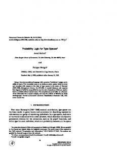
Here, the correct answer is an interval from 80 to 89%. All interval or point responses that lie between these boundaries are coherent probability assessments and we call them “coherent intervals” (or “coherent interval responses”). These boundaries are derived from the inequality given above. In Europe it is well known, that people from Alsace are very likely to speak both German and French. This can be regarded as a salient heuristic stereotype. To control this variable we presented our subjects a tourist party from England. Of this tourist party it is very untypical that there are many people that speak two languages. According to the Heuristics & Biases framework, subjects should infer higher values for the tourist party form Alsace compared with the tourist party from England. Our data did not support this hypothesis. The subjects used similar strategies for solving the problems and were not influenced by the representativeness heuristic that was varied in the premises. This is may be due to the fact that the subjects were asked to think hard. Let us stress that our tasks allow for investigating the lower probability bound: to our knowledge, the lower probability bounds have been neglected in the psychological literature (the conjunction fallacy is a violation of the upper bound only). The lower probability of P (A ∧ B) is greater than zero if P (A) + P (B) > 1. If P (A) = P (B) = .8, e.g., P (A ∧ B) ≥ (.8 + .8) − 1 = .6. Subjects’ lower bounds can be below, within, or above the coherent intervals, and the subjects’ upper bounds can be above, within or below the coherent intervals. Six possible categories of interval responses result (cf. Figure 1): too wide intervals (a), only the upper (b) or only the lower bound is coherent (c), the whole interval is below

13

(d) or above (f) the coherent interval (e). (a) (b) (d)

(c) (e)

(f)

0%

100% coherent interval

Figure 1: Categories of possible interval responses. Coherent interval responses (e). Incoherent interval responses: too wide intervals (a), intervals with both bounds too low (d) or too high (f), intervals where only the upper (b) or only the lower bound (c) are coherent. In our studies on the and-Rule we found a pattern of results that was consistent over all tasks. The mean frequency of coherent interval responses over all 14 tasks was 25.57 (n = 40, SD = 3.74). That is, 63.93% of the subjects responded coherently. Because the coherent category contains the majority of responses compared with the other five categories of the possible incoherent intervals, this may be interpreted as a good agreement of our subjects with the rationality norms. We found clearly more violations of the lower bound (frequencies in categories (b) and (d)) than of the upper bound. This is different from the results reported in the Heuristics & Biases tradition (Kahneman et al., 1982), where subjects committed upper bound violations (conjunction fallacies). Too wide intervals (category (a)) are rather seldom. For details see Pfeifer & Kleiter (2005a). The frequency of coherent responses does not depend upon the size of the normative interval: in one task, the coherent interval was 62-63% and 23 of 40 subjects responded coherently. In another task, the coherent interval was 28 times larger (35-63%) and again 24 of 40 subjects responded coherently. Besides the and Rule, we investigated the left logical equivalence, the right weakening, the or and the cautious monotonicity Rule of system p (Pfeifer & Kleiter, 2005a, 2005b, 2003; Pfeifer, 2002). In the left logical equivalence task 95% of the subjects (n = 20) responded coherent lower and coherent upper bounds. The result was replicated in a second experiment (Pfeifer & Kleiter, 2005a). A similar result was found in a study on the right weakening Rule where 90% of the subjects (n = 20) gave interval responses within the normative lower and upper bounds. 56.80% of these subjects gave the normative lower and the normative upper bounds (Pfeifer & Kleiter, 2005b). Thus, for both the left logical equivalence and the right weakening Rule good agreement was found between system p and the actual inferences of the subjects. 14

In another experiment, we compared the cautious monotonicity Rule with its “incautious” monotonic counterpart, the monotonicity Rule, that is not contained in system p. The second premise of the cautious monotonicity Rule (from α |∼ β and α |∼ γ infer α ∧ β |∼ γ) was omitted in the monotonicity condition (from α |∼ β infer α ∧ γ |∼ β). The investigation of the monotonicity Rule is of special interest, since—contrary to the rules of system p—only the non-informative unit interval, [0, 1], can be inferred whatever the probability value of the premise is. We found that our subject were sensitive to the non-informativeness of the monotonicity Rule: subjects inferred wide intervals with bounds relatively close to 0 and 100%. In accordance with our previous results, the data suggest that people reason nonmonotonically: the subjects in the cautious monotonicity condition inferred significantly tighter intervals and close to the coherent intervals compared with the subjects in the incautious monotonicity condition (Pfeifer & Kleiter, 2005b). Overall, we observed good agreement between the results and the predictions of the probability interpretation of system p. The results corroborated our hypothesis that nonmonotonic reasoning is a plausible candidate for modeling human reasoning. The conditionals of the form α |∼ β are associated with high probabilities. We think that this is the reason for our finding that humans tend to violate lower probability bounds more often as compared with upper bounds. The following list summarizes our studies on system p (Pfeifer & Kleiter, 2005a, 2005b, 2003): • Good overall agreement with system p • and Rule: – Far less upper bound violations (conjunction fallacies) than lower bound violations • Good agreement of the monotonicity and the cautious monotonicity rules: – Intervals of the monotonicity Rule are greater than cautious monotonicity Rule • or Rule: relatively good agreement • left logical equivalence Rule: very good agreement • right weakening Rule: very good agreement Our studies on the probabilistic interpretation of system p suggest nonmonotonic reasoning as a plausible candidate for a theory of human reasoning not only at the normative but also at the descriptive level.

15

3

Conditional Syllogisms

In this section we give four examples of probability logic “at work”. As we are not aware of empirical data of the probability logical versions of these examples, we focus on the formal aspects only. There are two probabilistic forms of the modus ponens depending on how the “if A then C” connective in the first premise is interpreted, whether (i) as a conditional propositions or (ii) as a material implication. The difference between the two interpretations was emphasized by Karl Popper long ago. We present the modus ponens and the modus tollens and two of their invalid counterparts in their conditional and material form. As mentioned above, the Probability Heuristics Model (Chater & Oaksford, 2004) is related but not equivalent to probability logic. Let A and C be propositions, “antecedent” and “consequent”, respectively. Modus ponens 1. Verity form A → C, A

⊢

C

(logically valid) .

2. Conditional proposition (Hailperin, 1996, p. 232) P (C|A) = p, P (A) = q

⊢

P (C) ∈ [pq, 1 − (1 − p)q] .

Numerical example: From p = .9 and q = .5 we conclude P (C) ∈ [.45, .95] . 3. Material implication (Hailperin, 1996, p. 203f) P (A → C) = p, P (A) = q

⊢

P (C) ∈ [max(0, p + q − 1), p] .

Numerical example: From p = .9 and q = .5 we conclude P (C) ∈ [.40, .90] . 4. Probability Heuristics Model (Chater & Oaksford, 2004) P (C|A) = 1 − ǫ , where ǫ is the probability of exceptions of the dependency between A and C. 5. The non-probabilistic modus ponens is actually endorsed by 89-100%7 of the subjects. 7

The percentages are taken from Evans et al. (1993, Table 2.4, p. 36), where seven studies of the non-probabilistic

(material) versions are summarized. Evans et al. selected studies w.r.t. broad similarity in procedure. 89% endorsement was found in a study with abstract material.

16

When P (A) = q = 1, that is, when the “instantiating data” are given for sure, the conditional proposition and the material implication intervals coincide. When both premises have the probability .5, then the material implication gives the interval [0, .5] while conditioning gives the symmetric interval [.25, .75]. The differences between the upper and the lower probabilities of both forms are the same, namely 1 + pq − p − q. Denying the antecedent 1. Verity form A → C, ¬A

6⊢

¬C

(not logically valid) .

2. Conditional proposition P (C|A) = p, P (¬A) = q

⊢

P (¬C) ∈ [1 − q − p(1 − q), 1 − p(1 − q)] .

Numerical example: From p = .9 and q = .5 we conclude P (¬C) ∈ [.05, .55] . 3. Material implication P (A → C) = p, P (¬A) = q

⊢

P (¬C) ∈ [1 − p, min(1 − p + q, 1)] .

Numerical example: From p = .9 and q = .5 we conclude P (¬C) ∈ [.10, .60] . 4. Probability Heuristics Model P (¬C|¬A) =

1 − b − aǫ . 1−a

5. The non-probabilistic denying the antecedent is endorsed by 17-73%8 of subjects. Affirming the consequent 1. Verity form A → C, C

6⊢

A (not logically valid) .

2. Conditional proposition P (C|A) = p, P (C) = q

⊢



P (A) ∈ 0, min



q 1−q , p 1−p



.

Numerical example: From p = .9 and q = .5 we conclude P (A) ∈ [0, .56]. The argument form requires a kind of “inverse probability”, reminding us at first sight of Bayes’ Theorem. Let A be a disease and C be a symptom. We know the conditional probability of 8

17% endorsement was found in a study with concrete material (Evans et al., 1993, p. 36).

17

the symptom given the disease, P (C|A), and the probability of the symptom to be present, P (A). What can we say about the probability of the disease? The answer is tricky. When the symptom probability q is greater than p and close to one, the probability interval of the disease is getting smaller and smaller and is finally approaching zero. The upper probability obtains a maximum when q = p. We see that affirming the consequent is actually very different from Bayes’ Theorem. 3. Material implication P (A → C) = p, P (C) = q

⊢

P (A) ∈ [1 − p, min(1, 1 + q − p)] .

Numerical example: From p = .9 and q = .5 we conclude P (A) ∈ [.10, .60]. 4. Probability Heuristics Model a(1 − ǫ) , b

P (A|C) = where a = P (A), b = P (C) and ǫ = P (¬C|A).

5. The non-probabilistic affirming the consequent is endorsed by 23-75% of subjects (Evans et al., 1993, p. 36). Modus tollens 1. Verity form A → C, ¬C

⊢

¬A (logically valid) .

2. Conditional probability (adapted from Wagner (2004, p. 751)) P (C|A) = p, P (¬C) = q

⊢

P (¬A) ∈ [z ′ , 1],

where, 

1−p−q p+q−1 , if 0 < p, q < 1, then z = max 1−p p ′ if (p = 0) ∧ (0 < q ≤ 1), then z = 1 − q , and ′



,

if (p = 1) ∧ (0 ≤ q < 1), then z ′ = q . Numerical example: From p = .9 and q = .5 we conclude P (¬A) ∈ [.44, 1]. 3. Material implication P (A → C) = p, P (¬C) = q

⊢

P (¬A) ∈ [max(0, p + q − 1), p] .

Numerical example: From p = .9 and q = .5 we conclude P (¬A) ∈ [.40, .90]. 18

4. Probability Heuristics Model P (¬A|¬C) =

1 − b − aǫ . 1−b

5. The non-probabilistic modus tollens is endorsed by 41-81% of subjects (Evans et al., 1993, p. 36). The conditional syllogisms are just a selection of simple argument forms. There are (infinitly) many others, of course. We note an interesting difference when the data are given for sure (q = 1). While in the conditional probability interpretation the conclusion holds with a probability of 1, in the material implication interpretation the conclusion holds with the probability of the rule only.

4

Categorical Syllogisms—Intermediate Quantifiers in Syllogistic Reasoning

There is an ongoing long tradition of psychological studies on classical syllogisms (Chater & Oaksford, 1999; Johnson-Laird, 1999; Bacon et al., 2003; Geurts, 2003; Newstead, 2003; Morley et al., 2004; Politzer, 2004). As with classical logic, we think that syllogistics is not an appropriate standard of reference for evaluating human reasoning. Specifically, the quantifiers involved in syllogistic reasoning are either too strict or too weak. On the one hand, the all-quantifier is too strict because it does not allow for exceptions—like the material implication! On the other hand, the existential quantifier is too weak because it quantifies only over (at least) one individual. Such quantifiers hardly ever occur in everyday life reasoning. Quantifications that—at least implicitly—actually occur in everyday life reasoning like “most . . . ”, “almost-all . . . ”, or “90 percent . . . ” are not expressible in traditional syllogistics. Since such quantifiers lie “in-between” the existential and the all-quantifier they are called intermediate quantifiers (Peterson, 2000). Intermediate quantifiers are promising candidates for investigating and evaluating human syllogistic reasoning. We do not have empirical data yet. We sketch a formal system of intermediate quantifiers to motivate empirical studies. Let us summarize briefly some facts about classical syllogisms. A syllogism is a two premise argument that consists of three out of four sentence types, or moods (Table 1). The order of the predicates involved is regimented by the four figures (Table 2). This leads to 256 possible syllogisms,9 of which 24 are 9 3

4 = 64 ways of constituting a two-premise argument (2 for the premises, 1 for the conclusion) by four moods (A, I, E,

19

Mood name

Notation

Read

Universal affirmative (A)

SaP

All S are P

Particular affirmative (I)

SiP

Some S are P

Universal negative (E)

SeP

All S are not P

Particular negative (O)

SoP

Some S are not P

Table 1: Moods involved in traditional syllogisms.

syllogistically valid. From a predicate logical point of view, only 15 syllogisms are predicate-logically valid. All 15 predicate logically valid syllogisms are also syllogistically valid. The reason is that in syllogistics you can deduce SiP from SaP , i.e.,

∀x(Sx → P x)

⊢syl

∃x(Sx ∧ P x)

This holds because in syllogistics it is implicitly assumed that the subject term Sx is not empty. This assumption is called “existential import”. In predicate logic, ∀x(Sx → P x) does not entail ∃x(Sx ∧ P x). The reason is well known: In predicate logic, formulae like ∀x(Sx → P x) can be “vacuously true”. This is the case when there is no x such that x has the property S, i.e., when the antecedent of the implication within the scope of the universal quantifier is “empty”. Then, clearly ∃x(Sx ∧ P x) is false (since ¬∃xSx is assumed). Hence,

∀x(Sx → P x)

0pl

∃x(Sx ∧ P x)

However, if we make an existential assumption explicit, we get:

∀x(Sx → P x) ∧ ∃xSx

⊢pl

∃x(Sx ∧ P x)

Do subjects make the existential import? How good are subjects in determining validity? Subjects are rather good at determining validity: the 24 valid syllogisms are judged as valid more often (51% of the time on average) than invalid syllogisms (11%; Chater & Oaksford (1999)). We reanalyzed the data summarized by Geurts (2003) and we distinguished syllogistic and predicate-logical validity. The distinction reveals that there is a higher percentage of endorsement with respect to all predicate logically valid O). Multiply 64 by the four figures gives 64 × 4 = 256 possible syllogisms.

20

Figure 1

Figure 2

Figure 3

Figure 4

Premise 1

MP

PM

MP

PM

Premise 2

SM

SM

MS

MS

Conclusion

SP

SP

SP

SP

Table 2: The four figures of syllogisms. S, M , and P are the subject, middle, and predicate term, respectively.

syllogisms (75.13%) than with respect to all syllogistically valid syllogisms (50.67%). Those syllogisms that are syllogistically but not predicate-logically valid are endorsed by only 9.89 % of the subjects. This is close to the percentage of the endorsement of all syllogistically invalid syllogisms (11%). This finding is counter-intuitive (why should subjects not make the existential import?). We don’t have an explanation. An important factor for the difficulty of a syllogism problem is the figure type: syllogisms of Figure 1 are the easiest, of Figure 4 the hardest, and those of figures 2 and 3 are in between (Geurts, 2003, p. 229). The two classical psychological theories of reasoning—the mental model theory (Johnson-Laird & Byrne, 1991; Johnson-Laird, 1999) and the mental rule theory (Rips, 1994; Braine & O’Brien, 1998)—try to explain these findings. Intermediate quantifiers are quantifiers “between” the all quantifier and the existential quantifier. Examples of intermediate quantifiers are Almost-all S are P, Most S are P, Many S are P or Fractionated quantifiers,

n m

S are P. We think that the traditional quantifiers are too strict to model human reasoning:

sentences of the form All S are P hardly ever occur in everyday life reasoning. Again, there are a priori grounds for preferring less strict quantifiers for modeling human reasoning. Intermediate quantifiers have hardly been investigated by psychologists. Exceptions are the logicbased approach by Geurts (2003) and Chater & Oaksford’s (1999) Probability Heuristics Model. We will not discuss these approaches here. Studies on probability judgment can be close to studies on fractionated quantifiers. Peterson (2000) provides algorithms to evaluate syllogisms with intermediate quantifiers. These algorithms are correct and complete with respect to arbitrarily many intermediate quantifier syllogisms ( 51 S are P,

2 5

S are P,

n m

S are P, . . . ). How are intermediate quantifiers interpreted? Consider the following

Venn diagram:

21

........ ........ ............. .................................... ................... ....... ...... ........... ..... ..... ..... ........ ..... ... ... .... ... ... . . ... ... .. .. . . ... ... .. .. . . ... .. .. ..... .... .. .. ... .. ... .. .. .. ................................. ... . ... . .. . . . . . . . . . . . ........ .. ....... ... . . . . . . . . . . ..... . ... .... .... . . . . . . . . . ... . ... ... . . . . . . . . . . ... ... ... .. .. ... ... ... ... .... .... ... .... .. ....... ..... .. ..... ......... ........ .......... ....... .... . . . . . . .............. . . . . . . . . . . . . . . . ............................ . ....................... ... .. ... ... ... .. ... .. . . ... . ... ... ... ... .... .... ...... ..... . ....... . . . . ............ ... .......................

S

P

b

a

c

e

f

d

h

g

M

S, M , and P represent the subject, middle, and predicate terms, respectively. Each term represents a class of objects (the S-class, the P -class, and the M -class). a, . . . , h label the cardinality of the eight possible subclasses of objects. Most S are P is then interpreted by the inequality b + e > a + d, where (b 6= 0 or e 6= 0). The “where . . .” clause makes the existential import explicit. Accordingly, Almost-all S are P is interpreted as b + e ≫ a + d,10 where (b 6= 0 or e 6= 0), and Many S are P is ¬(a + d ≫ b + e), where (b 6= 0 or e 6= 0). “Exactly

m n

n−m of the S are P ” is defined as “( m n of the S are P ) and ( n S are ¬P )” (Peterson, 2000, p.

208). Under this interpretation the traditional square of oppositions can be generalized as in Table 3. Lists of valid syllogisms with intermediate quantifiers and easy methods of proving their validity are given by Peterson (2000). Finally, we note that Peterson’s logic of intermediate quantifiers can easily be related to a probability interpretation based on relative frequencies. A difference between the Probability Heuristics Model of syllogistic reasoning and probability logic is whether independence assumptions are made or not. Chater & Oaksford (1999, p. 244) assume for their Probability Heuristics Model of syllogistic reasoning conditional independence: the end terms (subject and predicate term) are independent given the middle term. In probability logic, this assumption is not made.

5

Concluding Remarks

We have raised the fundamental question of the choice of an appropriate normative standard of reference for evaluating human reasoning. We tried to show why classical logic alone should not serve as a 10

“≫” is read as “greatly exceeds”.

22

Quantifier

Affirmative

Negative

Universal

A: All S are P

E: All S are ¬P

↓

↓

Predominant

P : Almost-all S are P

Majority

↓

↓

T : Most S are P

D: Most S are ¬P

↓

↓

...

...

↓

↓

S are P More-than- n−m n

More-than- n−m S are ¬P n

↓

↓

...

Fraction

(n

≥

B: Almost-all S are ¬P

2m)

m n

...

Common

Particular

m n

S are P

S are ¬P

↓

↓

...

...

↓

↓

K: Many S are P

G: Many S are ¬P

↓

↓

I: Some S are P

O: Some S are ¬P

Table 3: Generalized squares of opposition (Adapted from Peterson, 1985, pp. 351ff). The solid lines indicate contradictions, dashed contraries, dotted subcontraries, and arrows subalternations (i.e. immediate entailments), respectively. ¬ is the negation.

23

standard. Furthermore, we motivated the psychological advantages of subjective probability theory over objective probabilities. After introducing probability logic, we explored the nonmonotonic system p and summarized our empirical studies. Conditional syllogisms, like the modus ponens, were probabilitized in Section 3 in both versions, material and conditional. Finally, we presented categorical syllogisms with intermediate quantifiers, like the “most . . . ” quantifier. Stanovich & West (1999; 2000) found that more intelligent subjects are doing better in reasoning under certainty and uncertainty tasks than less intelligent subjects. Now, more intelligent subjects may be supposed to be more rational than less intelligent ones. Thus, the correlation between intelligence and performance may be taken as a supporting criterion that an appropriate normative model was chosen to evaluate performance. So why do we want to consider normative models that are weaker than those used to evaluate reasoning performance? Do the weaker models make errors in human reasoning to “disappear”? The answer is clearly no in the domain of reasoning under uncertainty. A conjunction fallacy remains a conjunction fallacy, neglecting base rates remains a neglect (Kleiter et al., 1997), etc. Though, it is not the same when probabilistic models are applied to “purely” logical tasks. Using a probabilistic model to Wason’s selection task does indeed lead to different “normative” solutions than using classical logic. The probabilities used in the probabilistic model were not mentioned in the task description given to the subjects. In our experiments we provided the subjects with the relevant probabilities. We do not want to completely discard classical logic as a normative standard of reference for human reasoning. This is obvious from the fact that subjective probability theory is based on the classical propositional calculus. In a similar way as probability theory presupposes propositional calculus na¨ıve probabilistic reasoning presupposes a basic understanding of crisp truth or falsity of propositions and of the elementary relationships between these truth values in a set of propositions. Moreover, if the premises are given for sure and known to be true, then we consider classical logic as the appropriate standard of reference. In everyday reasoning premises are nearly never known for sure, and then probability logic is the appropriate standards of reference. Probability logic represents the appropriate class of models to evaluate human inference under uncertainty. If “degrees of belief” really matter in human reasoning, then we should make them explicit in our models. The question whether humans are rational or not is not our main motivation (has it been a fruitful question after all?). The question is how to appropriately model reasoning under conditions of partial and incomplete knowledge and to trace descriptive theories of the according cognitive processes. That is what we mean by “mental probability logic”. 24

Probability logic is in no way restricted to such simple kinds of inferences. It is in fact a highly general approach to probabilistic inference. An alternatively powerful and general approach to probabilistic inference are graphical independence models. Bayesian networks are the best known subclass of these models. The variables instantiated by observations together with the probabilities and conditional independence relations build the premises. The remaining variables are candidates for conclusions. Actually, the role of the variables is not that simple and the formulation of probabilistic inference in Bayesian networks requires the properties of conditional independence, the theory of Markov properties, etc. A major difference between probability logic and graphical models is that in graphical models probabilities are assumed to be known while in probability logic the information may be incomplete. Thus, the usual graphical models process point probabilities and do not model imprecision.

References Adams, E. W. (1975). The logic of conditionals. Dordrecht: Reidel. Adams, E. W. (1998). A primer of probability logic. Stanford, CA: CSLI. Antoniou, G. (1997). Nonmonotonic reasoning. Cambridge, MA: MIT Press. Bacchus, N., Grove, A. J., Halpern, J. Y., & Koller, D. (1996). From statistical knowledge bases to degrees of belief. Artificial Intelligence, 87 (1-2), 75-143. Bacon, A. M., Handley, S. J., & Newstead, S. E. (2003). Individual differences in strategies for syllogistic reasoning. Thinking and Reasoning, 9 (2), 133-168. Benferhat, S., Bonnefon, J.-F., & Da Silva Neves, R. (in press). An overview of possibilistic handling of default reasoning, with experimental studies. Synthese. Benferhat, S., Saffiotti, A., & Smets, P. (2000). Belief functions and default reasoning. Artificial Intelligence, 122, 1-69. Biazzo, V., & Gilio, A. (1999, 29 June - 2 July). A generalization of the fundamental theorem of de Finetti for imprecise conditional probability assessments. In 1st international symposium on imprecise probabilities and their applications. Ghent, Belgium. Biazzo, V., Gilio, A., Lukasiewicz, T., & Sanfilippo, G. (2002). Probabilistic logic under coherence, modeltheoretic probabilistic logic, and default reasoning in System P. Journal of Applied Non-Classical Logics, 12 (2), 189-213.

25

Bonnefon, J.-F., & Hilton, D. J. (2002). The suppression of modus ponens as a case of pragmatic preconditional reasoning. Thinking & Reasoning, 8 (1), 21-40. Braine, M. D. S., & O’Brien, D. P. (Eds.). (1998). Mental logic. Mahwah, NJ: Erlbaum. Chater, N., & Oaksford, M. (1999). The probability heuristics model of syllogistic reasoning. Cognitive Psychology, 38, 191-258. Chater, N., & Oaksford, M. (2004). Rationality, rational analysis, and human reasoning. In K. Manktelow & M. C. Chung (Eds.), Psychology of reasoning. Theoretical and historical perspectives (p. 43-74). Hove and New York: Psychology Press. Coletti, G., & Scozzafava, R. (2002). Probabilistic logic in a coherent setting. Dordrecht: Kluwer. Da Silva Neves, R., Bonnefon, J.-F., & Raufaste, E. (2002). An empirical test of patterns for nonmonotonic inference. Annals of Mathematics and Artificial Intelligence, 34, 107-130. De Finetti, B. (1974). Theory of probability (Vols. 1, 2). Chichester: John Wiley & Sons. (Original work published 1970) Delgrande, J. P. (1988). An approach to default reasoning based on a first-order conditional logic: Revised report. Artificial Intelligence, 36, 63-90. Dubois, D., Lang, J., & Prade, H. (1994). Possibilistic logic. In D. M. Gabbay & C. J. Hogger (Eds.), Handbook of logic in artificial intelligence and logic programming. Oxford: Clarendon Press. Dubois, D., & Prade, H. (1988). Possibility theory. An approach to computerized processing of uncertainty. New York: Plenum Press. Evans, J. S. B. T. (1977). Linguistic factors in reasoning. Quarterly Journal of Experimental Psychology, 29, 297-306. Evans, J. S. B. T. (2002). Matching bias and set sizes: A discussion. Thinking and Reasoning, 8, 153-163. Evans, J. S. B. T., Handley, S. H., & Over, D. E. (2003). Conditionals and conditional probability. Journal of Experimental Psychology: Learning, Memory, and Cognition, 29, 321-355. Evans, J. S. B. T., Newstead, S. E., & Byrne, R. M. J. (1993). Human reasoning. Hove, UK: Erlbaum. Evans, J. S. B. T., & Over, D. E. (2004). If. Oxford: Oxford University Press. Ford, M. (2004). System LS: A three-tiered nonmonotonic reasoning system. Computational Intelligence, 20 (1), 89-108. Ford, M. (in press). Human nonmonotonic reasoning: The importance of seeing the logical strength of arguments. Synthese. Ford, M., & Billington, D. (2000). Strategies in human nonmonotonic reasoning. Computational Intelli26

gence, 16 (3), 446-468. Gabbay, D. M., & Hogger, C. J. (Eds.). (1994). Handbook of logic in artificial intelligence and logic programming (Vol. 3. Nonmonotonic reasoning and uncertain reasoning.). Oxford: Clarendon Press. Geurts, B. (2003). Reasoning with quantifiers. Cognition, 86, 223-251. Gilio, A. (2002). Probabilistic reasoning under coherence in System P. Annals of Mathematics and Artificial Intelligence, 34, 5-34. Goodman, I. R., Nguyen, H. T., & Walker, E. A. (1991). Conditional inference and logic for intelligent systems. A theory of measure-free conditioning. Amsterdam: North-Holland. G¨ardenfors, P., & Makinson, D. (1994). Nonmonotonic inference based on expectation orderings. Artificial Intelligence, 65, 197-245. Hailperin, T. (1996). Sentential probability logic. Origins, development, current status, and technical applications. Bethlehem: Lehigh University Press. Johnson-Laird, P. N. (1999). Deductive reasoning. Annual Review of Psychology, 50, 109-135. Johnson-Laird, P. N., & Byrne, R. M. J. (1991). Deduction. Hillsdale, NJ: Erlbaum. Kahneman, D., Slovic, P., & Tversky, A. (Eds.). (1982). Judgment under uncertainty: Heuristics and biases. Cambridge: Cambridge University Press. Kern, L. H., Mirels, H. L., & Jomsjaw, V. G. (1983). Scientists’ understanding of propositional logic: An experimental investigation. Social Studies of Sciences, 13, 131-146. Kleiter, G. D., Doherty, M. E., & Brake, G. (2002). The psychophysics metaphor in calibration research. In P. Sedlmeier & T. Betsch (Eds.), Frequency processing and cognition (p. 238-255). Oxford: Oxford University Press. Kleiter, G. D., Krebs, M., Doherty, M. E., Garavan, H., Chadwick, R., & Brake, G. (1997). So subjects understand base rates? Organizational Behavior and Human Decision Processes, 72 (1), 25-61. Kolmogoroff, A. N. (1933). Grundbegriffe der Wahrscheinlichkeitsrechnung. Berlin, Heidelberg, New York: Springer. Konolige, K. (1994). Autoepistemic logic. In D. M. Gabbay, C. Hogger, & H. Robinson (Eds.), Handbook of logic in artificial intelligence and logic programming: Nonmonotonic reasoning and uncertain reasoning (Vol. 3, p. 218-295). Oxford: OUP. Kraus, S., Lehmann, D., & Magidor, M. (1990). Nonmonotonic reasoning, preferential models and cumulative logics. Artificial Intelligence, 44, 167-207. Lehmann, D., & Magidor, M. (1992). What does a conditional knowledgebase entail? Artificial Intelli27

gence, 55 (1), 1-60. Lifschitz, V. (1994). Circumscription. In D. Gabbay, C. Hogger, & H. Robinson (Eds.), Handbook of logic in artificial intelligence and logic programming: Nonmonotonic reasoning and uncertain reasoning (Vol. 3, p. 297-352). Oxford: OUP. Marcus, S. L., & Rips, L. J. (1979). Conditional reasoning. Journal of Verbal Learning and Verbal Behavior, 18, 199-223. Markovits, H. (1988). Conditional reasoning, representation, and empirical evidence on a concrete task. Quarterly Journal of Experimental Psychology, 40A, 483-495. McCarthy, J. (1980). Circumscription: A form of non-monotonic reasoning. Artificial Intelligence, 13, 27-39. McDermott, D., & Doyle, J. (1980). Non-monotonic logic I. Artificial Intelligence, 13, 41-72. Moore, R. C. (1985). Semantical considerations on nonmonotonic logic. Artificial Intelligence, 25, 75-94. Morley, N. J., Evans, J. S. B. T., & Handley, S. J. (2004). Belief bias and figural bias in syllogistic reasoning. The Quarterly Journal of Experimental Psychology, 57 (4), 666-692. Newstead, S. E. (2003). Can natural language semantics explain syllogistic reasoning? Cognition, 90, 193-199. Nute, D. (1994). Defeasible logic. In D. Gabbay, C. Hogger, & H. Robinson (Eds.), Handbook of logic in artificial intelligence and logic programming: Nonmonotonic reasoning and uncertain reasoning (Vol. 3, p. 353-395). Oxford: OUP. Oaksford, M. (2002). Contrast classes and matching bias as explanations of the effects of negation on conditional reasoning. Thinking and Reasoning, 8, 135-151. Oaksford, M., & Chater, N. (1994). A rational analysis of the selection task as optimal data selection. Psychological Review, 101, 608-631. Oaksford, M., & Chater, N. (1998). Rationality in an uncertain world. Hove, GB: Psychology Press. Oaksford, M., Chater, N., & Larkin, J. (2000). Probabilities and polarity biases in conditional inference. Journal of Experimental Psychology: Learning, Memory, and Cognition, 26, 883-899. Oberauer, K., & Wilhelm, O. (2003). The meaning(s) of conditionals: Conditional probabilities, mental models and personal utilities. Journal of Experimental Psychology: Learning, Memory, and Cognition, 29, 680-693. Over, D. E., & Evans, J. S. B. T. (2003). The probability of conditionals: The psychological evidence. Mind & Language, 18, 340-358. 28

Pearl, J. (1988). Probabilistic reasoning in intelligent systems. San Mateo, CA: Morgan Kaufmann. Pearl, J. (1990). System Z. In M. Y. Vardi (Ed.), Proceedings of theoretical aspects of reasoning about knowledge (p. 21-135). Santa Mateo, CA: Morgan Kaufmann. Pelletier, F. J., & Elio, R. (2003). Logic and computation: Human performance in default reasoning. In P. G¨ardenfors, K. Kijania-Placet, & J. Wolenski (Eds.), Logic, methodology and philosophy of science. Dordrecht: Kluwer. Peterson, P. L. (2000). Intermediate quantifiers. Logic, linguistics, and Aristotelian semantics. Aldershot: Ashgate Publishing Company. Pfeifer, N. (2002). Psychological investigations on human nonmonotonic reasoning with a focus on System P and the conjunction fallacy. Unpublished master’s thesis, Institut f¨ ur Psychologie, Universit¨at Salzburg. (http://citeseer.nj.nec.com/pfeifer02psychological.html) Pfeifer, N., & Kleiter, G. D. (2003). Nonmonotonicity and human probabilistic reasoning. In Proceedings of the 6th workshop on uncertainty processing (p. 221-234). Hejnice: 24 - 27th September, 2003. Pfeifer, N., & Kleiter, G. D. (2005a). Coherence and nonmonotonicity in human reasoning. Synthese, 146 (1-2), 93-109. Pfeifer, N., & Kleiter, G. D. (2005b). Nonmonotonicity and human probabilistic reasoning. Unpublished manuscript. Universit¨at Salzburg, Fachbereich Psychologie. Politzer, G. (2004). Some precursors of current theories of syllogistic reasoning. In K. Manktelow & M. C. Chung (Eds.), Psychology of reasoning. Theoretical and historical perspectives (p. 213-240). Hove and New York: Psychology Press. Politzer, G., & Bourmaud, G. (2002). Deductive reasoning from uncertain conditionals. British Journal of Psychology, 93, 345-381. Pollock, J. (1994). Justification and defeat. Artificial Intelligence, 67, 377-407. Poole, D. (1980). A logical framework for default reasoning. Artificial Intelligence, 36, 27-47. Popper, K. R. (1994). Logik der Forschung. T¨ ubingen: Mohr Siebeck. (10. Aufl.) Ramsey, F. P. (1994). General propositions and causality (1929). In D. H. Mellor (Ed.), Philosophical papers by F. P. Ramsey (p. 145-163). Cambridge: Cambridge University Press. Reiter, R. (1980). A logic of default reasoning. Artificial Intelligence, 13, 81-132. R´enyi, A. (1955). On a new axiomatic theory of probability. Acta Mathematica Academiae Scientiarum Hungaricae, 6, 285-335. Rips, L. J. (1994). The psychology of proof: Deductive reasoning in human thinking. Cambridge, 29

Massachusetts: MIT Press. Rips, L. J. (2002). Reasoning. In H. Pashler & D. Medin (Eds.), Stevens’ handbook of experimental psychology, vol. 2: Cognition (3rd ed.). New York: Wiley. Rumain, B., Connell, J., & Braine, M. D. S. (1983). Conversational comprehension processes are responsible for reasoning fallacies in children as well as adults. Developmental Psychology, 19, 471-481. Schurz, G. (1997). Probabilistic default reasoning based on relevance and irrelevance assumptions. In D. Gabbay et al. (Ed.), Qualitative and quantitative practical reasoning (p. 536-553). Berlin: Springer. Schurz, G. (1998). Probabilistic semantics for Delgrande’s conditional logic and a counterexample to his default logic. Artificial Intelligence, 102, 81-95. Schurz, G. (in press). Non-monotonic reasoning from an evolution-theoretic perspective: Ontic, logical and cognitive foundations. Synthese. Stanovich, K. E. (1999). Who is rational. Studies of individual differences in reasoning. Mahwah, NJ: Erlbaum. Stanovich, K. E., & West, R. F. (2000). Individual differences in reasoning: Implications for the rationality debate? Behavioral and Brain Sciences, 23, 645-726. Stevenson, R. J., & Over, D. E. (2001). Reasoning from uncertain premises: Effects of expertise and conversational context. Thinking and Reasoning, 7, 367-390. Taplin, J. E. (1971). Reasoning with conditional sentences. Journal of Verbal Learning and Verbal Behavior, 12, 530-542. Touretzky, D. S. (1986). The mathematics of inheritance systems. Los Altos, CA: Morgan Kaufmann. Wagner, C. (2004). Modus Tollens probabilized. British Journal of Philosophy of Science, 55, 747-753. Yama, H. (2001). Matching versus optimal data selection in the Wason selection task. Thinking and Reasoning, 7, 295-311.

30