ing systems such as Linux and need for synchronized execu- ... When hardware failures occur, .... tion was given to mechanism for ensuring that the monitors.
Towards A Model-Based Autonomic Reliability Framework for Computing Clusters Abhishek Dubey
Steve Nordstrom Ted Bapty
Turker Keskinpala Gabor Karsai
Sandeep Neema
Institute for Software Integrated Systems Department of Electrical Engineering and Computer Science Vanderbilt University, Nashville, TN 37203, USA {dabhishe, steve-o, tkeskinpala, sandeep, bapty, gabor}@isis.vanderbilt.edu
Abstract One of the primary problems with computing clusters is to ensure that they maintain a reliable working state most of the time to justify economics of operation. In this paper, we introduce a model-based hierarchical reliability framework that enables periodic monitoring of vital health parameters across the cluster and provides for autonomic fault mitigation. We also discuss some of the challenges faced by autonomic reliability frameworks in cluster environments such as non-determinism in task scheduling in standard operating systems such as Linux and need for synchronized execution of monitoring sensors across the cluster. Additionally, we present a solution to these problems in the context of our framework, which utilizes a feedback controller based approach to compensate for the scheduling jitter in non realtime operating systems. Finally, we present experimental data that illustrates the effectiveness of our approach.
1. Introduction Reduced cost of commodity computers and the advent of high capacity networks have made cluster computing economical. Clusters are used for solving complex problems that traditionally required the use of a supercomputer [8, 3]. Their advantage lies in the ubiquity of their components commodity computers interconnected using high-speed networks such as Myrinet [22] and Infiniband [14]. This in turn delivers high performance computing at a fraction of price associated with supercomputers. However, only applications that can be parallelized by splitting into a number of smaller job-units can truly reap their benefits. Several such large computing clusters are maintained at Fermi National Accelerator Laboratory (FNAL), some
of which are primarily reserved for solving lattice quantum chromodynamics (LQCD) computations1 (see table 1). LQCD is a challenging field of study that employs largescale numerical calculations in order to extract fundamental parameters of the standard model of nuclear physics from experiments [11]. Table 1. FNAL LQCD clusters Cluster QCD PION KAON
CPU 2.8 GHz Pentium 4 3.2 GHz Xeon 2.0 GHz Dual Opteron
Nodes 127 518 600
OS Linux Linux Linux
One of the primary problems with clusters is to ensure that they maintain a working state most of the time to justify economics of operation. Unfortunately, reliability is not a prime design consideration for the hardware, operating systems, and middleware in commodity computers that are often built for higher performance per dollar. However, when these computers are used together in a cluster, reliable operation is expected. Large analysis campaigns like the ones involved in LQCD are composed of a number of inter-dependent tasks that have to be successfully performed to complete the full workflow2 . In such cases, failure of even a single node can halt progress on all nodes assigned to the job, resulting in loss of both time and money. These failures can be (but not limited to) power outages, hardware failures, nonresponsive job-units, or even ambient cooling failures. While applications can be written to be fault-tolerant, the development cost will be significantly greater and the performance lower. Instead, these applications are constructed 1 See
http://lqcd.fnal.gov/ workflow is a specification of a set of tasks or jobs to be performed, their execution order and their input/output dependencies 2A
for absolute performance. When hardware failures occur, an application-specific set of tasks have to be done. For some LQCD jobs, for example, the distributed job is killed and restarted from a checkpoint. If done manually, this approach can be expensive, slow to respond, and limit scalability. Instead, an autonomic approach is required that can ensure that the resources of the cluster are used to best possible extent and achieve the best possible start to completion ratio of jobs, even in the presence of hardware/software failures. Such a system will also improve response time in problem solving.
Figure 1. Overview of SCARF The Scientific Computing Autonomic Reliability Framework (SCARF), being developed by our research group for the LQCD computing clusters, is one such framework. Fig. 1 illustrates its conceptual architecture. The monitoring and mitigation portions of SCARF are based on the hierarchical Reflex and Healing (RH) framework, presented in [6, 18, 23, 20]. The basic components of this framework are distributed monitoring units, fault-mitigation units and a system wide planner for dealing with resource reallocation in case of severe failures. The primary monitoring units are sensor programs that execute periodically and ondemand across all nodes in the cluster. On the top is a design environment for deploying analysis campaigns and setting up monitoring and mitigation policies. The algorithm and components for the resource reallocation for a workflow have been presented in [19]. SCARF is a model-based reliability framework. It relies upon the use of a model-based specification of workflows, jobs, cluster resources and important monitoring parameters. It also provides for specification of models of mitigation policies based on a well-defined model of computations, along the same lines as those presented in [6]. Furthermore, it allows the realization of the monitoring and mitigation constituents of the framework using model transformations [12]. In this paper, we will present the monitoring portion of this framework. Primarily, the focus of this paper is con-
centrated on two main problems that affect SCARF’s performance. We can summarize them as follows: 1. Operating systems such as Linux, widely used in cluster environments, are designed for good average performance rather than worst-case performance. This leads to a non-deterministic task scheduling, which in turn causes any periodic job running on that node to accrue jitter between the expected start time and the actual start time. This jitter has detrimental effect on cluster management systems as they depend on periodic sampling and correlation of health status data from every node in the cluster. We will discuss this problem further in section 4.1. 2. Synchronization between the various periodic sensor programs running across the cluster is necessary to ensure execution of all instances happen at the same time on all nodes. This is required to prevent the worst-case scenario where a parallel application, waiting for synchronization across multiple nodes of the cluster, can be blocked forever. This can happen if at any time at least one of the nodes required for synchronization is not ready as it is executing the sensors of the reliability framework. This problem will be explained in further detail in section 4.2. It should be mentioned that these problems are generic in nature and will affect any reliability framework designed for large clusters. In the latter half of this paper, we will present solutions to these problems by (a) using a discrete event based sensor scheduler, and (b) employing a feedback controller based approach that compensates for the scheduling jitter in non-real-time operating systems. Additionally, we will also present experimental data that illustrates the effectiveness of our approach.
2. Related Research Generalized frameworks are being increasingly used to monitor the health and status of cluster resources. Early tools such as ClusterProbe [13] concentrate on per node monitoring and visualization without considering the health of the cluster as a whole. Many monitoring tools have been developed at centers for supercomputing at the national laboratories. NetLogger [9] was developed at the Lawrence Berkeley National Laboratory and provides high performance event logging channels for capturing status messages across clusters into a centralized location. The Monitoring and Managing Multiple Clusters (M3C) [2] was developed at Oak Ridge National Laboratory, which provides a web-based GUI administration tool that allows a human administrator to monitor parameters across a federation of clusters on
demand. Further developments of cluster management systems include the Java Agents for Monitoring and Management (JAMM) [25] system that was developed at Lawrence Berkeley National Laboratory to facilitate monitoring of more dynamic configurations of cluster environments using a publisher/subscriber methodology. These frameworks were tailored for centralized, human-in-the-loop management of clusters but little investigation was done to provide autonomic monitoring and control of cluster computing environments. OVIS [1] uses a more complex statistical method to deduce models for a cluster’s baseline status and provides a mechanism for automatic detection of early failures based on a node’s conformity to those models. However, the computational costs of this approach are intensive, and can have a detrimental effect on the available cluster resources. Other tools such as the RVision [7] monitoring system have been investigating the effects of the monitoring framework on the performance of the cluster. Metrics for measuring how the RVision monitoring system interferes with the performance of hosted cluster applications is given by Ferreto in [7]. While the results were promising, no special consideration was given to mechanism for ensuring that the monitors do not interfere with the applications. Moreover, no consideration is given to the necessary failure mitigation portions of a truly autonomic monitoring and control framework. In recent years, many modern frameworks such as Ganglia [17], Nagios [10] have been undergoing development. These frameworks are very well suited toward cluster monitoring and even simple control, and their open source licenses promote their use within the scientific community. While many of these frameworks are easily extended, they provide no mechanisms for bounding either the invocation time or execution time of components within the system beyond mechanisms given by the operating system. Nevertheless, there is a need for modern monitoring frameworks that considers the effect of non-determinism of commercial operating systems and compensates for the same.
3. An Introduction to SCARF Figure 1 shows the basic components of the framework: distributed monitoring units, fault-mitigation units and a system wide planner for dealing with workflow re-planning. The benefit of using the model-based approach is the possibility of policy verification as presented earlier in [5, 6]. In this paper, we will be limiting the description to the monitoring and mitigation portions. This framework employs a hierarchical network of decentralized fault management entities called reflex engines. A reflex engine comprises of several state machines, which change states and perform actions associated with the transitions upon occurrence of certain predefined events. Fig. 2
Figure 2. Implementing the reliability framework using hierarchical reflex engines.
shows the deployment of reflex engines in the framework. To manage scalability, all reflex engines are divided into three logical hierarchical levels, which are global, regional and local. Fig. 2 describes the hierarchical aspect of SCARF. Local managers are the closest to a worker node in the cluster. In response to a mitigation command given by a superior level manager, they can deploy or remove various sensors on their node or even make changes in the configuration, such as a change in periodicity of a particular sensor. These sensors provide monitoring for different health parameters. In effect, they realize the “system health monitor” block from Fig. 1. Local managers are also responsible for actuating the necessary mitigation action dictated by the regional manager. Regional managers supervise and communicate with a number of subordinate managers that are in their area of observation. They also store all the sensory information received from their subordinates in a database to be used for historical correlation in future. A regional manager has a wider area of observation and can correlate diagnosis to ascertain if a problem is common to a number of user applications and take coordinated mitigation action. Together, the local and regional managers realize the fault-mitigation engine block from Fig. 1. The head node of the cluster is usually designated as a single global manager and is used as a resource planner and the gateway to submit new jobs or plan the resources assigned to an existing job.
3.1. Sensors The primary fault-detection entities are sensor programs, which periodically execute on the nodes in the cluster. Data is channeled from the sensors to the local manager, which sends it to the regional manager, where a built-in state machine is used for fault detection. This flow of data is achieved by using Syslog-ng - a next generation version of the popular protocol Syslog used for the transmission of
event notification messages across networks [15]. The faultmitigation commands are sent by the regional manager to a local manager by using UDP. In this case, UDP is preferred over TCP as it is stateless and does not require dedicated socket connections between the two managers, saving precious network bandwidth. Fig. 3 illustrates this dataflow.
Table 2. Sensors in the framework No. 1 2 3 4 5 6 7 8 9 10 11 12 13 14
Sensor CPU Fanspeed Motherboard Fanspeed CPU Temperature Motherboard Temperature Aggregate CPU Utilization CPU Utilization per process Hard Disk Utilization RAM and Swap Utilization Aggregate RAM Utilization Aggregate Swap Utilization CPU Voltage Motherboard Voltage Monitor configuration changes Heartbeat
Period(sec) 10 10 10 10 10 10 10 10 10 10 10 10 60 300
Figure 3. Dataflow of messages exchanged between managers
Table 2 contains the list of 14 sensors currently running on all nodes in the Pion and Kaon cluster (refer to table 1). One of the most critical sensors is the heartbeat sensor. It indicates the health of a node. If more than one contiguous heartbeat is missed then the regional manager checks the health of the node by sending pings to the local manager. If the ping is ignored, it marks the node in question as dead and reallocates its part of the job to another node. Readers are referred to [19] for the algorithm of workflow re-planning in case of faults. A special sensor (number 13 in table 2) is employed to reload the executable code of other sensors if a configuration change is detected in their respective source code, for example, when the local manager changes the periodicity of sensors running on that node. Function of other sensors is obvious from their name. These sensors (except heartbeat) only report the value if it is over or below a certain threshold to reduce network traffic. This threshold is decided based on the historical correlation between faults and health parameter values at that time. Since the sensors execute frequently, it is necessary that they are least intrusive i.e. the average CPU utilization due to sensor measurements should be minimal. In order to achieve this, the scheduler to run these sensors is based on a technique presented in [4] used for simulating discrete event systems. This scheduler is implemented as a single process with one thread to ensure the small CPU load, which executes periodically.
3.2. Sensor Scheduler Algorithm 1 describes a typical discrete-event based scheduling algorithm as seen from the perspective of a single node. All periodic sensor programs have two variables,
a time period (P ) that is constant for a given sensor, and a current clock value (C) that is initialized to the respective time period (P ) of that sensor. The prominent feature of this algorithm is the scheduling step in which the time for the next scheduled iteration is set. This time is set by making the sensor scheduler sleep for a time T , which is decided by evaluating the current clock values (C) of all sensors. Sleep can be realized in standard operating systems, such as Linux, either by a system call or by using an alarm signal and an appropriate signal handler [24]. On any given operating system, the resolution of sleep implementation used in the sensor scheduler determines the minimum periodicity that can be set for a sensor program. Algorithm 1 Sensor scheduler Input: S {Set of periodic sensors. Each sensor has two variables: P(Time period), C (current clock Value)} Pre Condition: (∀s ∈ S)(s.C = P ) 1: loop 2: Set T = minimum((∀s ∈ S)(s.C) 3: Set Alarm for T {Alarm can be implemented by sleep or using signals in both Linux and Windows} 4: (∀s ∈ S)(s.C ← s.C − T ) 5: (∀s ∈ S)(s.C = 0 =⇒ Execute(s)) 6: (∀s ∈ S)(s.C = 0 =⇒ (s.C ← s.P )) 7: Run any aperiodic sensors if present. 8: end loop
At the start of an iteration, clock values of all sensor programs are decremented by the current value of sleep time, T . Subsequently, the scheduler runs any sensor program that has a zero clock value and updates its clock value to the respective time period. Here we wish to distinguish two distinct terms, iteration of the sensor scheduler and the sensor runs. The iteration is the periodic tick of the sensor scheduler, while a sensor run
happens when the sensor scheduler executes the program of a sensor during iteration. Note that the precision of the periodicity for sensors completely depends upon the accuracy of the sleep function provided by the operating system. However, in many cases the standard Linux kernel provides no upper bound on the difference between the actual time of sleep compared to the requested time. In the next section, we will discuss the problems caused by this reality.
4. Problem due to Jitter and Synchronization 4.1. Jitter One of the foremost problems faced in a monitoring framework is the timeliness of sensor readings. Ideally, the nodes in the framework should have a real-time operating system (RTOS) to guarantee the performance and timeliness of sensor readings. However, usually clusters are built with standard version of Linux kernel as the chosen operating system, which is geared towards best average-case performance than the worst-case performance. Consequently, the standard Linux kernel does not guarantee deterministic task scheduling. Non-deterministic scheduling can lead to unbounded jitter between the expected and actual time of the sensor reading and make the task of analysis engines even more difficult. This problem has been studied earlier by P. Marti et. al in [16]. They showed that the jitter can not only lead to performance degradation but can also lead to instability. For example, the regional managers cannot wait forever to determine the absence of a heartbeat from worker nodes. They have bounds on the maximum time that they can wait for before a mitigation action is executed. Consequently, false alarms might be issued if the heartbeat does not arrive within the stipulated time. Moreover, unbounded jitter in sensor readings will eventually lead to a large skew in timestamps of observation that were taken at the same time. This can cause problems in analysis, where a global snapshot of the state of cluster at any particular time might be required. In order to formalize the notion of jitter, consider a generic periodic task τ with a time period T . The ideal release time of such a task would be a sequence < kT >k=∞ k=1 relative to some time, tφ . Let s(kT ) be the start time of k th instance of this task such that the start is delayed by tj(kT ) with respect to the expected start time, tφ + kT . Then total jitter, tj(kT ) = s(kT ) − kT − tφ . Now, consider the k + 1th instance of the same task. If the schedule is set by using sleep for T time, like in line 3 of algorithm 1, then it can be seen that the relative time difference between the two start times is greater than the time period,
s((k + 1)T ) − s(kT ) ≥ T . In such a case, the total jitter will keep accumulating and increase with time. At any point, tj(kT ) will represent all the delays accumulated over time till that point and will be equal to the absolute relative jitter until that instance, which is defined as the maximum deviation between start time and the expected start time among all the instances of a periodic task. Figure 4 illustrates the effect of accumulating jitter. From the figure we can see that if nothing is done the sensor measurements will always be off from the expected time by some value. Two problems arise when this phenomenon of delayed sensor readings is seen from the perspective of the cluster: (a) sensor measurements are not exactly periodic any more. This affects analysis routines that rely on uniform sampling rate of sensor readings; (b) sensors are run at different times on the nodes of the cluster. This affects the performance of jobs that needs to synchronize across the cluster. We explain this problem in detail in the next subsection.
Figure 4. Periodic sensing will accumulate delay when used in a standard OS.
4.2. Synchronization Issue A programming model commonly followed in LQCD computing cluster jobs is Multiple Instruction Stream and Multiple Data Stream (MIMD). In this model, different nodes execute in parallel on different data streams. However, the computation results from various nodes have to synchronize together in order to solve for boundary conditions. For example, in LQCD cluster an application called MILC3 (MIMD Lattice computation collaboration) has to do a global synchronization at a rate of every 45 milliseconds. The requirement is that all nodes in the job must be ready at the time of synchronization i.e. the scheduler on each of those nodes should not be running any other task at that time, otherwise the job is delayed till all the nodes are ready. 3 http://physics.indiana.edu/
˜sg/milc.html
Figure 6. Relationship between a hyperperiod and ticks. Figure 5. Loss in the performance of a MILC job when run in the presence of unsynchronized sensor schedulers across the cluster.
In the current setup, on an average a sensor takes 30 milliseconds for measurement. Moreover, to ensure fairness MILC jobs and the sensor scheduler runs with the same priority. Therefore, it is possible that a sensor run is scheduled such that it preempts the run of MILC task on the node and delays the global synchronization. In the worst case, it might be possible that at any time there is always at least one sensor running on a node, which will preempt the global synchronization of the MILC job across all nodes. In that scenario, the MILC job will be stalled forever. However, in average case we will see a performance drop because of the extra time spent by the MILC job in waiting for the synchronization. For example, Fig. 5 illustrates the drop in MFLOPS achieved from an actual computing job executed across 256 nodes when the unsynchronized sensor framework was brought online on the cluster. In this figure, MILC GFTIME is the name of the application executing on the cluster. It can be seen that the performance of the job drops from around 400 MFLOPS to 300 MFLOPS when the sensor schedulers comes online across the whole cluster.
5. Solution Approach Synchronization and jitter are two interdependent issues. Even if the sensor schedulers across the cluster are started at the same time, they will soon go out of sync because of the inherent jitter. Therefore, the solution for the two problems required an integrated approach. For this, we divide the time scale into hyperperiods and ticks between the hyperperiod as described in Fig. 6. The ticks are instances in time when the sensor scheduler runs a sensor if its current clock value is zero (refer to algorithm 1). If more than one sensor is eligible for execution then the order of run must
be deterministic. A lexical sort on their names is one way of achieving this determinism. The start of the hyperperiod is the time when all sensor schedulers across the cluster reset their clocks and start a new cycle of sensor runs. In effect, this forces them to resynchronize at the start of each hyperperiod. The behavior of all sensor schedulers is such that they must wait for the hyperperiod signal when starting for the first time. One of the existing facilities of Linux operating system is the Network Time Protocol (NTP). By using the global manager as the NTP server, we can ensure that wall clock times of all nodes in the cluster are within a few milliseconds of each other. This provides for an opportunity to use a set time of day as the hyperperiod signal across the cluster. For experimental purposes, we chose every 300 second of the day as the hyperperiod. It should be noted that this decision requires a trade-off. If a very fine hyperperiod is used, say 20 seconds, the performance of the cluster will be reduced. However, if a very coarse hyperperiod is chosen, say 20 minutes, then there will be a large accumulation of jitter between hyperperiod synchronizations. Between any two hyperperiods, the sensor scheduler uses the sleep to space out the ticks for sensor runs. However, even with this hyperperiod synchronization it is possible to accumulate jitter between the expected and actual time of the tick. In effect, this will lead to many unsynchronized sensor runs between the hyperperiod synchronizations. This is why we need a mechanism to control the uniformity of ticks.
5.1. Plant and Controller Model Let T be the minimum time period in algorithm 1. Also, let tj(kT ) be the total jitter accumulated at the kth sensor run. Assume a disturbance d(kT ) that has been accrued till this run due to scheduling activity and finite time taken
by sensors for completing their execution. In a standard operating system, there will be no guaranteed bound on this disturbance. Based on the discussion in this paragraph we can write the difference equation for the plant as : tj((k + 1)T ) = tj(kT ) + d(kT )
(1)
This is the discrete-time state space equation that we will use as our plant model. The state variable in this equation is the total jitter at any time sample, tj(kT ). Now onwards, we will drop the term kT and just use k as the index term.
For this design, we chose a PI controller. The derivative term was dropped because the sudden and frequent changes in the disturbance value would have made the feedback loop unstable. Given that the state space variable is total jitter, tj(k) and the reference value is zero, we can write the error signal as e(k) = −tj(k). The plant and controller equations are: tj(k + 1) = tj(k) + d(k) + c(k), where c(k) = −K[tj(k) +
5.2. Feedback Controller One of the basic feedback configurations is the proportional, integral and derivative (PID) scheme. Basic principle of the PID control scheme is to act on the control variable through a combination of proportional action, integral action and the derivative action. The proportional action is proportional to the error signal, which is the difference between reference input and the feedback signal. Integral action is proportional to integral of error signal and the derivative action is proportional to the derivative of the error signal. In our case, the plant is a discrete-time system with a sample time, T . The principle of PID control scheme applies to such systems as well. The difference is that the integral and derivative components are approximated by trapezoidal summation and difference equation respectively. In [21], the discrete-time PID controller equation is given as:
c(k) =K[e(k) +
j=k T X e(j − 1) + e(j) + Ti j=1 2
Td [e(k) − e(k − 1)]] T
j=1
tj(j − 1) + tj(j) ] 2
(3) (4)
Figure 8. An equivalent block diagram of the control loop shown in Fig. 7. Dashed box indicates the control loop Now, we apply the Z-transformation [21] to both sides of equation 4. Note that we follow the notation of representing discrete-time domain variables with small alphabets, and use the capital alphabets for the corresponding Zdomain value. For example, X(z) = Z[x(k)]. Ki ]T J(z), where (1 − z −1 )
(5)
Ki is the effective proportional gain 2
(6)
C(z) = −[Kp + (2)
T Ti
j=k X
Kp = K − Ki =
KT is the integral gain Ti
(7)
Redrawing the block diagram presented in Fig. 7 as Fig. 8, we can show that the transfer function of this feedback controller is: T F (z) = Figure 7. The feedback control loop for the sensor scheduler
Here, T is the sampling time period, e is the error signal, c is the controller output, K is the proportional gain, Td is the derivative time constant and Ti is the integral reset time constant. Fig. 7 shows this control loop.
1 1 + [Kp +
Ki (1−z −1 ) ]
(8)
For stability, poles of T F must lie within the unit circle in z-domain or |z| < 1 [21]. From equation 8, the characterKi istic equation for finding the poles is 1+[Kp + (1−z −1 ) ] = 0. 1+K
p Therefore, the pole is at z = 1+Kp +K . Since Kp and Ki i are real, the stability criterion implies −(1 + Kp + Ki ) < (1 + Kp ) < (1 + Kp + Ki ). This equation upon simplification yields the condition Ki > 0, or K > 0 (ref equation 7).
Alternatively, in other words the sufficient stability criterion is that the chosen proportional gain is positive.
5.3. Modified Sensor Scheduler with Synchronization and Feedback Controller Algorithm 2 shows the algorithm with the modification made for synchronization and feedback controller to sensor scheduler presented earlier in section 3.2. Note that the feedback controller is executed between two hyperperiods. In each hyperperiod, synchronization is achieved by sleeping till the next hyperperiod. The number of ticks between two hyperperiods is computed by dividing hyperperiod width by the length of a tick and taking its greatest lower bound. The variable tj stores the current value of the total jitter . Iterm is used to calculate the integral component of the feedback compensation in accordance with equation 4. The maximum compensation that can be provided is limited by the value of timeperiod (T) (see line 13 of the algorithm). This is done because sensor scheduler cannot sleep for negative times.
can be applied to other periodic applications that control their own release time by maintaining their own clock. For periodic applications that do not control their own release, or are directly invoked by the kernel, we can incorporate a dummy scheduler with feedback controller between the kernel scheduler and the application.
6. Results In this section, we will present results obtained by implementing the sensor scheduler with feedback loop i.e. algorithm 2. All these experiments use a value of K = 1.0 and Ki = 1.2.
6.1. Experiment1: Performance of feedback controller in controlling jitter.
Algorithm 2 Modified sensor scheduler with synchronization and feedback controller to compensate for jitter Input: S {Set of periodic sensors by name. Each sensor has two variables: P(Time period), C (current clock Value). T is the greatest common factor of sensor time periods.} Input: HY P ER {the Hyperperiod value} 1: S ← Sort(S) 2: loop 3: Use nanosleep() to sleep till the next Hyperperiod signal Pre Condition: (∀s ∈ S)(s.C = P ) 4: Initialize T imeStamp1 ← CurrentT ime() { CurrentTime() returns the current time in the system} 5: Initialize Iterm ← 0 {Integral Term} 6: Count ← F loor(HY P ER/T ) {Floor provides the greatest lower bound integer.} 7: for I = 0 to Count do 8: T imeStamp2 ← CurrentT ime() 9: d(k − 1) ← T imeStamp2 − T imeStamp1 − T {k − 1 because the disturbance is from the last step.} 10: tj(k) ← tj(k − 1) + d(k − 1) 11: Iterm ← Iterm + (tj(k − 1) + tj(k))/2 12: Set T = minimum((∀s ∈ S)(s.C) 13: c(k) ← −(min(T, Ki ∗ Iterm + K ∗ tj(k))) 14: nanosleep(T + c(k)) {nanosleep is a higher resolution sleep function available in Linux} 15: (∀s ∈ S)(s.C ← s.C − T ) 16: (∀s ∈ S)(s.C = 0 =⇒ Execute(s)) 17: (∀s ∈ S)(s.C = 0 =⇒ (s.C ← s.P )) 18: Run any aperiodic sensors if present. 19: end for 20: end loop
The controller and plant model developed here is not specific to this sensor scheduler framework. On the contrary, it
Figure 9. Total jitter accumulated in last 9 hours. Fig. 9 shows the total jitter accumulated by the sensor scheduler’s main feedback loop running over a period of 9 hours. For this test, the sample time period was set as 5 seconds to make it more susceptible to disturbances. It was found that the root mean square (RMS) value of the jitter was 0.2243 after 9 hours, only 4.4% of the sampling time period, 5 seconds. This demonstrates the effectiveness of the feedback loop in controlling periodic jitter.
6.2. Experiment2: Jitter with and without controller with changing CPU Load In order to emulate the step response of this controller, we decided to create a step disturbance by loading the CPU in steps to the 100% capacity manually. For this purpose, we used a number of prime number generators freely available over the internet to load the CPU. Furthermore, to emulate the step response, we initially started the framework without the controller, and then started the controller
(a) Performance with synchronized sensor scheduler
(b) Performance without synchronization. This is a restatement of Fig. 5, reproduced here for ease in comparison.
Figure 10. Improved performance of a MILC job with synchronized sensor scheduler. at a predefined time, in this case the 21st run of the sensor scheduler. Fig. 11 shows the result of this experiment. Notice that the total jitter rises initially when the controller is off. It settles down with a few oscillations when the controller is switched on. This figure also illustrates the contrast in jitter with and without the controller. The RMS value of total jitter in steady state was 0.209 seconds. This shows that the total jitter was bounded even when the system was heavily loaded.
Figure 12. Time take during each iteration.
Figure 11. Plot of total Jitter with varying CPU Load. The controller was switched on at 155th second (dotted line).
6.3. Experiment3: Performance of MILC Job- synchronization problem This test was conducted on 128 nodes in the pion cluster. All instances of sensor schedulers were started from
the head node in parallel . After the launch, sensor schedulers synchronized to the next plus one 5th minute of the hour. In this case, that time was ’Fri Oct 19 09:45:10 2007 (call it base time). Then onwards the sensor scheduler used the feedback controller for iterating every 10 seconds till the next hyperperiod. Sensors were run during an iteration based on their clock value. Lexical order was used to ensure that a deterministic order of sensor runs. Overall, 14 sensors ran on the nodes (see table 2). The test was stopped after 584 iterations with a sampling time of 10 seconds. On an average 12 sensors ran during all iterations. 13th sensor (monitoring changes in sensor codes) was executed in every 6th iteration, while 14th sensor (heartbeat) ran every 30th iteration. Fig. 12 shows the time taken during all sensors. Notice that 95.3% of the sensor runs took less than 500 millisec-
onds for the measurement. Recall that the sensor run is the execution of a sensor program during an iteration of the sensor scheduler. The excess time taken during some sensor runs can be attributed to the non-deterministic scheduling provided by the operating system. Fig. 10 shows the performance drop in the MILC job when synchronized sensor schedulers were switched on in the cluster. Compare figure 10(a) to the earlier result without synchronized sensor scheduler in Fig. 5,restated for comparison as figure 10(b). We can see that, on an average, there is a 50 MFLOPS gain in the performance compared to before. We can attribute the still existing performance drop of 50 MFLOPS to the 500 milliseconds taken on an average in a sensor run, which can still block the synchronization task. However, since the sensor schedulers are synchronized we do not see an accumulated delay in the MILC job as before. During this experiment, the average CPU utilization over a period of 24 hours on one of the nodes due to Sensor Scheduler was found to be 0.024 percent. The corresponding RAM utilization value was 0.318 percent.
[2]
[3]
[4]
[5]
[6]
7. Conclusion and Future works In this paper, we presented a reliability framework for clusters called SCARF that implements this feedback controller based synchronization technique. Experiments presented in the previous sections show that the reduction of total jitter is possible with the use of the feedback controller presented in this paper. Moreover, the use of feedback controller only imposed a trivial amount of extra CPU load. This along with the hyperperiod synchronization allows all sensor runs across the cluster to execute simultaneously. Consequently, the performance drop in parallel jobs with the sensor framework present was reduced. Future investigations will include the semantics of the modeling language to help deploy the analysis routines along with the required monitoring framework. We will also investigate the automatic synthesis of workflows to be deployed on the cluster from a given analysis specification. Our goal is to achieve a holistic framework that enables deployment of workflows along the cluster and manages the health of the cluster to maximize its efficiency.
8. Acknowledgments This work is supported by the National Science Foundation under the ITR grant ACI-0121658. The authors will also like to acknowledge their colleagues at Fermi National Accelerator Laboratory.
References [1] J. Brandt, A. Gentile, D. Hale, and P. Pebay. Ovis: a tool for intelligent, real-time monitoring of computational clus-
[7]
[8]
[9]
[10] [11] [12]
[13]
[14]
[15] [16]
ters. In Parallel and Distributed Processing Symposium, 2006. IPDPS 2006. 20th International, page 8pp., 25-29 April 2006. M. Brim, A. Geist, B. Luethke, J. Schwidder, and S. Scott. M3c: managing and monitoring multiple clusters. In Cluster Computing and the Grid, 2001. Proceedings. First IEEE/ACM International Symposium on, pages 386–393, 15-18 May 2001. R. Buyya. High Performance Cluster Computing: Architectures and Systems. Prentice Hall PTR, Upper Saddle River, NJ, USA, 1999. C. G. Cassandras and S. Lafortune. Introduction to Discrete Event Systems. Kluwer Academic Publishers, Norwell, MA, USA, 1999. A. Dubey, S. Nordstrom, T. Keskinpala, S. Neema, and T. Bapty. Verifying autonomic fault mitigation strategies in large scale real-time systems. In EASE ’06: Proceedings of the Third IEEE International Workshop on Engineering of Autonomic & Autonomous Systems (EASE’06), pages 129– 140, Washington, DC, USA, 2006. IEEE Computer Society. A. Dubey, S. Nordstrom, T. Keskinpala, S. Neema, T. Bapty, and G. Karsai. Towards a verifiable real-time, autonomic, fault mitigation framework for large scale real-time systems. Innovations in Systems and Software Engineering, 3:33–52, March 2007. T. Ferreto, C. de Rose, and L. de Rose. Rvision: An open and high configurable tool for cluster monitoring. In Cluster Computing and the Grid, 2002. 2nd IEEE/ACM International Symposium on, pages 75–75, 21-24 May 2002. Z. Fodor, S. D. Katz, and G. Papp. Better than $1/mflops sustained: a scalable pc-based parallel computer for lattice qcd. Computer Physics Communications, 152:121, 2003. D. Gunter, B. Tierney, B. Crowley, M. Holding, and J. Lee. Netlogger: a toolkit for distributed system performance analysis. In Modeling, Analysis and Simulation of Computer and Telecommunication Systems, 2000. Proceedings. 8th International Symposium on, pages 267–273, 29 Aug.-1 Sept. 2000. R. C. Harlan. Network management with nagios. Linux Journal, 2003(111):3, 2003. D. J. Holmgren. PC clusters for lattice qcd, 2004. ´ L´edeczi, and T. Bapty. ModelG. Karsai, J. Sztipanovits, A. integrated development of embedded software. Proceedings of the IEEE, 91(1):145–164, 2003. Z. Liang, Y. Sun, and C.-L. Wang. Clusterprobe: an open, flexible and scalable cluster monitoring tool. In Cluster Computing, 1999. Proceedings. 1st IEEE Computer Society International Workshop on, pages 261–268, 2-3 Dec. 1999. J. Liu, A. Vishnu, and D. Panda. Building multirail infiniband clusters: Mpi-level design and performance evaluation. In Supercomputing, 2004. Proceedings of the ACM/IEEE SC2004 Conference, pages 33–33, 2004. C. Lonvick. The BSD syslog protocol, 2001. P. Mart´ı, J. M. Fuertes, K. Ramamritham, and G. Fohler. Jitter compensation for real-time control systems. In RTSS ’01: Proceedings of the 22nd IEEE Real-Time Systems Symposium (RTSS’01), page 39, Washington, DC, USA, 2001. IEEE Computer Society.
[17] M. L. Massie, B. N. Chun, and D. E. Culler. The ganglia distributed monitoring system: design, implementation, and experience. Parallel Computing, 30(5-6):817–840, 2004. [18] S. Nordstrom, T. Bapty, S. Neema, A. Dubey, and T. Keskinpala. A guided explorative approach for autonomic healing of model based systems. In Second IEEE conference on Space Mission Challenges for Information Technology (SMC-IT), July 2006. [19] S. Nordstrom, A. Dubey, T. Keskinpala, R. Datta, S. Neema, and T. Bapty. Model predictive analysis for autonomicworkflow management in large-scale scientific computing environments. In EASE ’07: Proceedings of the Fourth IEEE International Workshop on Engineering of Autonomic and Autonomous Systems, pages 37–42, Washington, DC, USA, 2007. IEEE Computer Society. [20] S. Nordstrom, S. Shetty, S. K. Neema, and T. A. Bapty. Modeling reflex-healing autonomy for large scale embedded systems. Systems, Man and Cybernetics, Part C, IEEE Transactions on, 36(3):292–303, 2006.
[21] K. Ogata. Discrete-time control systems (2nd ed.). PrenticeHall, Inc., Upper Saddle River, NJ, USA, 1995. [22] Y. Qian, A. Afsahi, and R. Zamani. Myrinet networks: a performance study. In Network Computing and Applications, 2004. (NCA 2004). Proceedings. Third IEEE International Symposium on, pages 323–328, 2004. [23] S. Shetty, S. Nordstrom, S. Ahuja, D. Yao, T. Bapty, and S. Neema. Systems integration of large scale autonomic systems using multiple domain specific modeling languages. In ECBS, pages 481–489, 2005. [24] A. Silberschatz and P. B. Galvin. Operating System Concepts. Addison-Wesley Longman Publishing Co., Inc., Boston, MA, USA, 1997. [25] B. Tierney, B. Crowley, D. Gunter, J. Lee, and M. Thompson. A monitoring sensor management system for grid environments. Cluster Computing, 4(1):19–28, 2001.