TOWARDS A MORE REALISTIC IONOSPHERIC MAPPING FUNCTION M. Hern´andez-Pajares, J. M. Juan, J. Sanz, M. Garc´ıa-Ferna´ ndez Res. group Astron. & Geomatics, Techn.Univ.Catalonia, gAGE/UPC Mod. C3 Campus Nord UPC, Jordi Girona 1-3, E08034 Barcelona (Spain) Contact e-mail:
[email protected] (
[email protected])
ABSTRACT The purpose of this work is to summarize the first results in order to get a more realistic and practical ionospheric mapping function. It is deduced exclusively from ground GPS data worldwide distributed (from IGS network) where the mean electron density in ionospheric voxels is estimated without using any background model. We demonstrate in this way that it is possible to get realistic and persistent estimates of the ionospheric effective height from ground GPS data which are in good agreement with the corresponding values deduced from independent GPS occultation data. Such validation is performed during 2002 coinciding with available GPS occultation receiver data of the Low Earth Orbiter (LEO) SAC-C. Such characterization of the effective height deduced from ground worldwide GPS data can be extended to representative datasets of the last Solar cycle, and the potential improvement in terms of ionospheric determination and corrections will be also discussed. INTRODUCTION The particular relationship between slant and vertical total electron content (TEC) -the ionospheric mapping functionis one of the first assumptions to consider typically when ionospheric corrections are estimated or applied from Global Navigation Satellite System (GNSS) data. On one hand it depends at a given time on the 3D electron content distribution and varies in terms of local time, latitude, season, Solar cycle epoch or ionospheric activity. But on the other hand, and for the sake of easiness, the typical assumption in many GNSS imaging and navigation systems is to consider a fixed mapping function constant, and associated to a 2D distribution of electron content at a given effective height (typically some value between 300 and 500 km). This can introduce, as it has been demonstrated by several authors a significant, and some times very important mismodelling that can affect to different applications such as global VTEC determination (see for example [1]) and precise navigation (shown in [2]). TOMOGRAPHIC ESTIMATION AND VALIDATION OF THE EFFECTIVE HEIGHT The purpose of this work is to show the feasibility of estimating a more realistic (and accurate) mapping function at global scale, in terms of variable GPS ionospheric effective height (hereinafter GIEH), from dual frequency GPS ground stations. This will be done using a Ionospheric Voxel model (hereinafter IVM), contemplating several shells or layers, solved by means of Kalman filtering of geometry-free carrier phase measurements. This can provide the relative vertical distribution of electron content which leads to estimating the corresponding effective heights. The IVM approach has shown its greater accuracy in previous works in both global scale VTEC determination and real-time ionospheric determination supporting accurate GPS navigation (see for instance [3]). In order to validate such GIEH estimation, an independent dataset and tomographic technique will be used: dual frequency data in occultation scenario (with negative elevations) gathered from the SAC-C LEO GPS receiver during 2002 (see for instance [4]) which provides vertical accurate electron density profiles by applying the improved inverse Abel transform (hereinafter IIAT, see for instance [5]). From each complete density profile, a GIEH value is derived and compared with the corresponding estimate from the IVM solution obtained from global ground GPS data. In both cases the corresponding GIEH has been derived, neglecting the horizontal VTEC gradient among
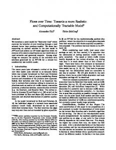
Iono. Effective height determination: ground vs. occultation data
GPS Effective Ionospheric Height / km
750
Ground data & 3-layers (@ 250-550-850 km) Ground data & 2-layers (@ 300-700 km) SAC-C data (electron density profiles)
700 650 600 550 500 450 400 350 300 250 258
259
260
261
262
263
264
GPS Time / days of 2002
Figure 1: Validation of Ionospheric effective height determined from global ground GPS data compared to values derived from electron density profiles computed from SAC-C LEO data (days 258-263 of 2002). other assumptions, by means of the following expressions 1 and 2: M=
S ' V
Z
T RA REC
X Pi r N 1 p i dh ' 2 − p2 V cos X V r i i
h= √
M p − re M2 − 1
(1)
(2)
being M the mapping function computed for a ray of impact parameter p (p is taken corresponding to receiver elevation of 20 deg), S the Slant Total Electron Content (STEC), V the Vertical TEC, X is the zenithal angle at the the given height, N the electron density, Pi and ri the partial TEC and geocentric distance corresponding to the i-th layer, and p is the ray impact parameter and re is the Earth radius. Finally to say that h represents the GPS ionospheric effective height (also known as ionospheric shell height) defined by means of equation 2: It corresponds to a thin layer fitting to the estimated mapping by tomographic techniques by equation 1. Such value is typically higher than the hmF2 values due to the topside electron content included in h definition. DATASETS, COMPUTATIONS AND RESULTS The main comparison presented in this manuscript is performed for six consecutive days (days 258-263 of year 2002) of both global ground IGS data (about 160 permanent selected stations each day) and LEO SAC-C occultation data (about 1600 occultations), still corresponding to the more difficult Solar and Seasonal Maximum conditions. In figure 1 you can see the GPS Ionospheric effective height obtained from IVM runs with ground data with different vertical layout: 2 layers (@ 300-700 km height) and 3 layers (@ 250-550-850 km height). Similar results are obtained with 10 layers (@ 100 to 1000 km height). It can be seen that such determinations are quite compatible between then and with the value deduced from SAC-C data. Both vary mostly due to the periodic change in Local Time, and latitude, along the LEO orbit.
180˚ 90˚
225˚
270˚
315˚
0˚
45˚
90˚
135˚
180˚ 90˚
60˚
60˚
30˚
30˚ 600
0˚
0˚
-30˚
-30˚
600
-60˚
-60˚ 400
-90˚ 180˚
225˚
270˚
315˚
0˚
45˚
90˚
135˚
-90˚ 180˚
07.0UT.heff02261 400
500
600
Figure 2: Example of GPS Ionospheric Effective height (in kilometers) computed from global IGS data for 0700UT, day 261 of 2002. As examples you can see typical snapshots of the effective height and VTEC estimations in figure 2 and 3 respectively (0700 UT, day 261, 2002). It can be seen in particular the known increase of effective height at the beginning and last part of the night, compatible with variations predicted by climatological ionospheric model, such as IRI (see [6]). Such increase is more important at low latitudes, and show a bimodal pattern, around the magnetic equator, before the sunrise. CONCLUSIONS AND FUTURE WORK We have shown in the manuscript the feasibility of estimating reliable ionospheric effective heights from ground GPS measurements, providing a way to get more realistic and accurate mapping functions for GPS users. Such estimates have been validated with electron density profiles deduced independently from SAC-C GPS occultation data. The corresponding global maps, computed in real-time, could potentially help on ionospheric communication issues. This study should be extended to get a characterization of the variable effective height mapping function to a significant part of a Solar cycle, in order to be able to establish a more realistic and accurate mapping function for the GNSS ionospheric users. Moreover, the potential advantage of using the partial to total electron content ratio instead of the effective height description (equation ??), should be considered as well in the future. ACKNOWLEDGMENTS The authors acknowledge to the International GPS Service and JPL the availability of the ground and SAC-C data sets respectively. This work has been partially supported by the Spanish project ESP-2004-05682-C02-01.
180˚ 90˚
225˚
270˚
315˚
0˚
45˚
90˚
135˚
180˚ 90˚
400
60˚
60˚
0
20
30˚
800
30˚
1000 600 1200
0˚
0˚
60
40
0
0
400
-30˚
-30˚ 400
200
200
-60˚
-60˚
-90˚ 180˚ 0
225˚ 100
200
270˚ 300
315˚ 400
500
0˚ 600
45˚ 700
90˚ 800
135˚
-90˚ 180˚
07.0UT.test02261 900
Figure 3: Total Electron Content (in tenths of TECU) snapshot computed simultaneously to the effective height map shown in the previous figure (0700UT, day 261 of 2002). REFERENCES [1] Hern´andez-Pajares, M., Juan, J.M. and Sanz, J, New approaches in global ionospheric determination using ground GPS data, Journal of Atmospheric and Solar-Terrestrial Physics, Vol.61, p. 1237-1247, 1999. [2] Hern´andez-Pajares, M., Juan, J.M., Sanz, J, and O.L. Colombo, Precise Ionospheric Determination and its Application to Real-Time GPS Ambiguity Resolution, proceedings of the ION-GPS’99 meeting, Nashville, TE, USA, Sept.1999. [3] Hern´andez-Pajares, M., Juan, J.M. and Sanz, J, Improving the real-time ionospheric determination from GPS sites at Very Long Distances over the Equator, Journal of Geophysical Research - Space Physics, Vol.107, p.12961305, 2002. [4] http://www.gsfc.nasa.gov/gsfc/service/gallery/fact sheets/spacesci/sac-c.htm [5] Hern´andez-Pajares, M. , Juan, J.M. and Sanz, J., Improving the Abel inversion by adding ground GPS data to LEO radio occultations in ionospheric sounding, Geophysical Research letters, Vol 27, No 16 pp 2473-2476. [6] A. Komjathy and R.B. Langley, The Effect of Shell Height on High Precision Ionospheric Modelling Using GPS, Proceedings of the 1996 IGS Workshop International GPS Service for Geodynamics (IGS), pp. 193-203, Workshop in Silver Spring, MD, 19-21 March 1996.