towards a structured consequential modelling approach for the ...

Faculty of Applied Engineering Research group Energy and Materials in Infrastructure and Buildings

TOWARDS A STRUCTURED CONSEQUENTIAL MODELLING APPROACH FOR THE CONSTRUCTION SECTOR: THE BELGIAN CASE A fairy tale on methodological choices in LCA

Thesis submitted in fulfilment of the requirements for the degree of doctor in Applied Engineering at University of Antwerp Matthias BUYLE

Promotor:

Prof. dr. ir. Amaryllis Audenaert

Antwerp, 2018

Members of the jury Prof. dr. Ing. Tom Breugelmans

Chair

University of Antwerp – faculty of Applied Engineering Research group Advanced Reactor Technology (ART) Prof. dr. ir. Amaryllis Audenaert

Promotor

University of Antwerp – faculty of Applied Engineering Research group Energy and Materials in Infrastructure and Buildings (EMIB) Dr. ir.-arch. Wim Debacker

Member of jury

Flemish institute for technological research (VITO) Prof. dr. Steven Van Passel

Member of jury

University of Antwerp – faculty of Applied Economics Department Engineering Management Prof. dr. Søren Løkke

Member of jury

Aalborg University (DK) - Department of Development and Planning Research Danish Centre for Environmental Assessment Prof. dr. ir. -arch. Karen Allacker

Member of jury

KU Leuven - Department of Architecture Research group Architectural Engineering Prof. dr. ir. Pieter Billen

Secretary

University of Antwerp – faculty of Applied Engineering Research group Biochemical Green Engineering & Materials (BioGEM)

iii

Acknowledgements I would like to thank my supervisor Amaryllis Audenaert for her substantial support, comments and advise throughout the entire journey. Thank you for introducing me in the field of Sustainability Assessment. I am grateful for the chances to learn so many different and new things. And more importantly, to get the opportunity to follow my personal research interests. Amaryllis, this research would not have been possible without you. Also, I would like to ‘put into the flowers’ my two other travel companions Wim & Wim (a.k.a. IDC-members). Wim Debacker, thanks for the endless interesting discussions and your valuable feedback. Even though we approach LCA slightly different, after every meeting at the comfy sofas in Berchem, I always went home full of ideas and renewed motivation. Wim Van den bergh, thank you for being such a nice chairman and I really enjoyed our profound e-mail conversations. Special thanks go to Massimo Pizzol and the rest of the Aalborg University crew. Massimo, thanks for the cooperation and all the support throughout the last three years. During my research stay in Aalborg you showed me what a positive experience doing research in an international context with like-minded people can be! I really appreciate your honest and critical opinion. Your comments were always spot on, which was sometimes confronting, yet they were always constructive. Since I know you really appreciate my writing skills, I like to thank you with this chaotic paragraph! Thanks to everyone who provided data or contributed in another way. I like to thank Waldo and the rest of the æ-lab (VUB) for their contributions to the last chapter on demountable and reusable walls. I hope we can continue this interesting collaboration. I thank the informal Sustainability Assessment group at the University of Antwerp for the collaboration. The crash course project writing last year was really helpful for finishing this manuscript. Also special thanks go to all jury members for their critical remarks, constructive suggestions and the stimulating discussion. I would like to thank all my (former) colleagues of the last eight years, for being such a nice team. In particular I’d like to thank my ‘roommates’ over the years: Lut, Wim, Jan, Giovanni, Joke, Ian, Karolien, Leen, Stijn, Stijn, Sravani, Alex, Imran and Pieter. Ian, thanks for keeping up the good spirits (pun intended) and the sports breaks. Finally, special thanks go to my two LCA-partners-in-crime, Joke and Giovanni. It has been a long and bumpy road for all three of us and for me personally, I don’t know if it was possible to make this journey completely on my own. I also would like to thank my friends and family. Arne, thanks for your significant contribution to the Poisson regression analysis. I’m very grateful to my parents for providing all the chances they’ve given me over the years. Special thanks for my father, for endless proofreading efforts and assisting me at drawing flow-charts that did not violate the basic laws of logic anymore. I also like to thank my grandfather posthumously for

v

proofreading my fist attempts of writing academic papers. These memories mean a lot to me. Finally, I owe many thanks to my favourite three women. Fenja, thanks for enduring my nagging and complaining over the years! And also a bit for all the support, patience and love of course. Abbi, thank you for your proofreading efforts! Your drawings on the draft versions improved the final result significantly. And Syra, together with Abbi, thanks for drawing my attention away from this work. Only this way I could keep things together during these last months. Matti Buyle, May 2018

vi

Abstract TOWARDS A STRUCTURED CONSEQUENTIAL MODELLING APPROACH FOR THE CONSTRUCTION SECTOR: THE BELGIAN CASE A fairy tale on methodological choices in LCA Considering its substantial contribution to the total global energy consumption and its use of raw materials, the construction sector is a clear target for improvement on the way to a more sustainable society. In the last decades, the focus of research and policy broadened from the initial objective of reducing energy consumption of a building in use to a more comprehensive approach that accounts for a building’s entire life cycle, for example by performing a life cycle assessment (LCA). Yet, despite the existence of general frameworks, still many assumptions and methodological choices have to be made throughout an LCA study. In this research, the focus is on consequential LCA, an approach which aims to describe how environmentally relevant flows will change in response to possible decisions. For example to opt for a timber frame instead of a traditional masonry structure. Despite its relevance is generally acknowledged, there is a lack of studies targeting the construction sector following a consequential modelling approach. In addition, its application is often done in a non-systematic and inconsistent way. So in this context, the goal of this work is to assess how consequential LCA can assist in improving the environmental profile of the construction sector, from materials to entire buildings. In other words, how can consequential LCA be applied on a consistent and transparent way across different products and product systems relevant for the construction sector, while maintaining consistent modelling choices? Building on the theoretical framework of Weidema et al. a practical method was developed that facilitates the transition from theory to practice and that is specific and detailed but ensures general applicability and practical feasibility. The central concept of this method is to identify the suppliers that are likely to be affected by a change in demand, i.e. the marginal suppliers. The method describes procedures to identify geographical market boundaries and subsequently the suppliers the most sensitive to a change in demand, based on their production trends. Also different perspectives on development can be included, reflecting past trends or expected future developments. Finally, the proposed method was applied and tested on three cases. In the first case the Belgian electricity grid mix is assessed. The possibilities of the proposed method were explored and used to further optimise the method. The second case focuses on the validation of the method and quantifying the effect of making modelling choices, by analysing a selection of six building products supplied to the Belgian market. While in the last case, demountable and reusable wall designs were evaluated on their environmental performance and compared with conventional designs.

vii

This work demonstrates that it is not only relevant to include a consequential modelling approach in LCA to improve the environmental profile of residential buildings, but also practically feasible to do it in a consistent and structured way. Even though making specific modelling assumptions can affect the results to a great extent, by explicitly accounting for this model uncertainty, more robust results can be obtained to support decisions.

viii

Samenvatting NAAR EEN GESTRUCTUREERDE CONSEQUENTIAL MODELERINGSAANPAK VOOR DE CONSTRUCTIE SECTOR: CASUS BELGIË. Een sprookje over methodologische keuzes in LCA De bouwsector heeft een substantieel aandeel in het totale wereldwijde verbruik van energie en grondstoffen. In het streven naar een duurzamere samenleving is dit dus een gegeven dat niet over het hoofd gezien mag worden. In de afgelopen decennia verschoof de focus in onderzoek en beleid van het verminderen van het energieverbruik naar een meer alomvattende aanpak die rekening houdt met de volledige levenscyclus van een gebouw, bijvoorbeeld aan de hand van een levenscyclusanalyse (LCA). Er bestaat een algemeen theoretisch kader voor het uitvoeren van een LCA-studie, maar per studie moeten er nog steeds aannames en methodologische keuzes gemaakt worden. In dit onderzoek ligt de nadruk op consequential LCA, een benadering die tracht om de milieueffecten in te schatten als gevolg van een beslissing. Bijvoorbeeld de keuze voor een houtskelet i.p.v. een traditionele gemetste structuur. Hoewel de relevantie van consequential LCA over het algemeen erkend wordt, werd dit tot op heden amper op een systematisch en consistente uitgevoerd binnen het bouwgerelateerde onderzoek. In deze context is het doel van dit werk om te evalueren hoe consequential LCA gebruikt kan worden bij het verbeteren van het ecologisch profiel van de bouwsector, van bouwmaterialen tot en met integrale gebouwen. Met andere woorden, hoe kan consequential LCA op een systematische en transparante manier worden toegepast op verschillende producten en productiesystemen die relevant zijn voor de bouwsector? Voortbouwend op het theoretisch kader van Weidema et al. werd er een praktische methode ontwikkeld die tracht de omzetting van theorie naar praktijk te vereenvoudigen en die tegelijkertijd specifiek, gedetailleerd en algemeen toepasbaar is. Het centrale concept van deze methode is het identificeren van producenten die beïnvloed kunnen worden door een veranderende vraag voor een zeker product. Deze producenten worden ook wel de marginal suppliers genoemd. De methode beschrijft procedures om geografische marktgrenzen en de producenten die het meest gevoelig zijn voor een dergelijke veranderende vraag te identificeren op basis van hun productietrends. Bovendien kunnen er verschillende ontwikkelingsperspectieven in rekening gebracht worden, gebaseerd op trends uit het verleden of verwachte ontwikkelingen. Ten slotte werd de ontwikkelde methode toegepast en getest op drie casussen. In het eerste geval wordt de Belgische elektriciteitsnetmix geanalyseerd. De mogelijkheden van de methode werden verkend en gebruikt bij de verdere optimalisatie ervan. De tweede casus richt zich op de validatie van de methode zelf en het kwantificeren van de effecten van verschillende modelleringskeuzes. Dit gebeurde op basis van zes bouwproducten, verdeeld op de Belgische markt. In de laatste cases worden de milieuprestaties van ix

ontwerpen van demonteerbare en herbruikbare binnenwanden beoordeeld en vergeleken met conventionele ontwerpen. Dit werk toont aan dat het niet alleen relevant is om een consequential model te integreren in LCA om acties te evalueren ter verbetering van het ecologisch profiel van woningen, maar dat het ook praktisch haalbaar is om dit op een consistente en gestructureerde manier te doen. Specifieke modelleringskeuzes kunnen het resultaat van een LCA-studie in grote mate beïnvloeden, maar door expliciet rekening te houden met deze modelonzekerheid, kunnen robuustere resultaten worden verkregen om zo gefundeerde beslissingen te kunnen nemen.

x

Table of contents Members of the jury........................................................................................................ iii Acknowledgements .........................................................................................................v Table of contents ............................................................................................................ xi Terminology .................................................................................................................. xv 1 INTRODUCTION ......................................................................................................... 1 Context ............................................................................................................ 1 1.1.1 Towards a more sustainable building stock.......................................... 1 1.1.2 Sustainability assessment....................................................................3 1.1.3 Responsibility paradigms.................................................................... 4 1.2

Objectives and research questions .................................................................. 6

1.3

Outline of the thesis ......................................................................................... 7

2 FROM BUILDING TO SUSTAINABLE BUILDING ......................................................... 9 2.1

LCA in the construction sector (until 2012) ..................................................... 10 2.1.1 Introduction ...................................................................................... 10 2.1.2 A brief history .................................................................................... 11 2.1.3 LCA methodology ............................................................................. 12 2.1.4 Developments in the construction sector .......................................... 15 2.1.5 Discussion and limitations ................................................................ 22 2.1.6 Research opportunities...................................................................... 23 2.1.7 Conclusion........................................................................................ 24

2.2 LCA in the construction sector - revisited (after 2012) .....................................25 2.2.1 Introduction ......................................................................................25 2.2.2 Developments in the construction sector ..........................................25 2.3

Consequential LCA ......................................................................................... 30 2.3.1 Introduction ...................................................................................... 30 2.3.2 Why, what and how? ......................................................................... 31 2.3.3 Marginal supplier identification ......................................................... 33

2.4 Conclusion ..................................................................................................... 36 3 EXPLORATORY CASE STUDIES ................................................................................ 37 3.1

Exploratory case 1. Optimising the environmental profile of dwellings ........... 38 3.1.1 Introduction ...................................................................................... 38 3.1.2 Methods ........................................................................................... 42 3.1.3 Results .............................................................................................. 47 3.1.4 Discussion ......................................................................................... 51 3.1.5 Conclusions .......................................................................................52 3.1.6 Insights and opportunities ................................................................. 53 xi

3.2

Exploratory case 2. the Belgian electricity mix ................................................ 55 3.2.1 Introduction ...................................................................................... 55 3.2.2 Methods ............................................................................................ 56 3.2.3 Results .............................................................................................. 63 3.2.4 Discussion ......................................................................................... 71 3.2.5 Conclusion ........................................................................................ 72 3.2.6 Insights and opportunities ................................................................. 73

4 ON A QUEST FOR A STRUCTURED METHOD........................................................... 75 4.1

Introduction ................................................................................................... 76

4.2 From a state of the art theoretical framework towards a practical method ..... 77 4.2.1 Identifying the scale and time horizon of the potential change studied .............................................................................................. 77 4.2.2 Identifying the limits of a market ....................................................... 78 4.2.3 Identifying trends in the volume of a market ..................................... 79 4.2.4 Identifying suppliers most sensitive to a change in demand .............. 80 4.3

General structure method .............................................................................. 81

4.4 Identification of geographical market boundaries .......................................... 83 4.4.1 General procedure ............................................................................ 83 4.4.2 Time effect ........................................................................................ 85 4.5

Identification of market volume trends and sensitive suppliers .......................86

4.6 Perspective on development .......................................................................... 87 4.7

Validation and sensitivity analysis of defining geographical market boundaries ..................................................................................................... 88 4.7.1 Definition market volume .................................................................89 4.7.2 Time effect ........................................................................................89 4.7.3 Comparison with other models .........................................................90

4.8 Conclusion ..................................................................................................... 91 5 OPTIMISATION, VALIDATION & APPLICATION ....................................................... 93

xii

5.1

Case 1. Building products ............................................................................... 95 5.1.1 Introduction ...................................................................................... 95 5.1.2 Methods ............................................................................................96 5.1.3 Results ..............................................................................................99 5.1.4 Discussion ....................................................................................... 115 5.1.5 Conclusions ..................................................................................... 116

5.2

Case 2. Internal walls designed for change ....................................................117 5.2.1 Introduction .....................................................................................117 5.2.2 Methods .......................................................................................... 119 5.2.3 Results ............................................................................................ 129 5.2.4 Discussion ....................................................................................... 135

5.2.5 Conclusion....................................................................................... 141 5.3

Discussion and Conclusion ............................................................................ 143 5.3.1 Data collection ................................................................................ 143 5.3.2 Implementation and evaluation ....................................................... 146 5.3.3 Practical recommendations ............................................................. 150

6 CONCLUSION AND OUTLOOK ............................................................................... 153 6.1

Research findings & achievements ............................................................... 154

6.2 Added value & strengths .............................................................................. 158 6.3

Limitations & reservations ............................................................................ 159

6.4 Research recommendations & opportunities ................................................ 160 References .................................................................................................................... 165 Figures and tables ......................................................................................................... 178 List of figures ........................................................................................................ 178 List of tables ......................................................................................................... 179 Appendices ................................................................................................................... 181

xiii

Terminology Abbreviations AIC

Akaike Information Criterion

ALCA

Attributional life cycle assessment

C&DW

Construction and demolition waste

CE

Circular economy

CEN TC 350

European Committee for Standardization - Technical Committee 350 “Sustainability of construction works”

CLCA

Consequential life cycle assessment

ENTSO-E

European Network of Transmission System Operators for Electricity

EPBE

Environmental profile of building elements (also known as MMG or Totem)

EPD

Environmental Product Declaration

EOL

End-of-life

FU

Functional unit

GGBFS

Ground granulated blast-furnace slag cement

GHG

Greenhouse gas

ISO

International Organization for Standardization

LCA

Life cycle assessment

LCEA

Life cycle energy assessment

LCI

Life cycle inventory

LCIA

Life cycle impact assessment

MENA

Middle East and North Africa region

nZEB

Nearly zero energy building

PEF

Product Environmental Footprint

PEM

Partial equilibrium model

RES

Renewable energy sources

SETAC

Society of Environmental Toxicology and Chemistry

TBL

Triple bottom line

TRL

Technology readiness level

xv

Glossary Avoided products

See ‘Product substitution’

Constrained suppliers/activity

An activity/supplier that is limited in its ability to change its production volume in response to a change in demand for its product output

Determining products

Product output of an activity for which a change in demand will affect the production volume of the activity. Also referred to as ‘reference product’.

Dependent by-products

Product from a unit process with multiple outputs that is not a determining product.

Marginal supplier

A supplier/producer that will change production capacity in response to a change in demand for a product (increase or decrease)

Market boundary

The spatial and temporal delimitation of a market

System expansion

A procedure for eliminating by-products as activity, thereby including the additional functions related to the by-products and modelling the resulting changes (substitutions) in the product system, especially by including the reduction in supply of the same product from the marginal supplier to the market for the by-product

Product substitution

A replacement of one product or group of products with another product or group of products that are functionally equivalent

Recycled content

The portion of materials used in a product that have been diverted from the solid waste stream

Recycling potential

The portion of materials that can substitute primary materials on the market when a product is disposed. Additional treatment can be required before functional equivalence is reached between the secondary and the substituted primary materials.

Reference flow

A quantified amount of product(s), including product parts, necessary for a specific product system to deliver the performance described by the functional unit

A comprehensive version of this glossary can be found at: https://consequential-lca.org/glossary/ (accessed on March 28, 2018)

xvi

1 1 INTRODUCTION “Answer that and stay fashionable” AFI

CONTEXT 1.1.1

TOWARDS A MORE SUSTAINABLE BUILDING STOCK

“Sustainable development is development that meets the needs of the present without compromising the ability of future generations to meet their own needs” [1, p.54]. Is there a better way to start a doctoral dissertation on environmental assessment than with one of most cited quotes in this field? This definition was introduced in the report “Our Common Future” by Gro Harlem Brundtland back in 1987 as a result of the UN Conference on the Human Environment in Stockholm (Sweden). Later on the importance of the concept of sustainable development - or sustainability in general - was broadly acknowledged and many other more detailed definitions were proposed (see [2]), yet still no consensus is Chapter 1. Introduction | 1

reached at this point. Nonetheless, it is commonly accepted that sustainability encompasses three domains of value, represented by its environmental, social and economic dimension. This is often referred to as Triple Bottom Line (TBL), a term coined by John Elkington in 1994 [3], or as People Planet Profit/Prosperity (PPP or 3P). A whole evolution has taken place since the publication of the Brundtland report. In the European Union the legal framework Energy Performance of Buildings Directive (EPBD) came into effect in 2006 and was revised in 2010 [4,5]. The revision shifted the focus from simply achieving some reductions in energy consumption to establishing ‘nearly zero energy buildings’ (nZEB). In addition, the attention for the materials used and their waste treatment increased, which resulted among others in the development of Construction Product Regulations and the implementation of the European Waste Framework [6,7]. At the same time efforts were undertaken to overcome the divergent interests of economic and environmental prosperity by introducing an alternative to the make-use-dispose paradigm, often referred to as circular economy (CE) [8,9]. The CE endeavours to extend the useful service life of products and promotes recycling and reuse [10,11].To achieve that goal, the potential of all components and materials should be fully utilized. This will lower environmental impact and resource consumption. The European Commission has set goals within its Circular Economy Package to stimulate the transition. These include a target for the recycling of municipal solid waste (e.g. minimum 65% of all waste by 2030) and for the landfilling of solid waste (e.g. maximum 10% of all waste by 2030) [10,11]. More specific to the construction sector, 70% of the non-hazardous construction and demolition has to be recycled or recovered by 2020 [7]. Against this background, it is clear there are many opportunities in the construction sector to contribute to a more sustainable society. The construction sector is responsible for nearly 40% of global energy consumption, 30% of raw material use, 25% of solid waste production, 25% of water use, 12% of land use and 33% of related global greenhouse gas (GHG) emissions [12,13]. In Flanders households have a share of 36–40% of the total energy consumption and the residential sector in Belgium produces about 40% of the emitted CO2 [14,15]. Based on these figures, it is clear that both energy and material consumption contribute substantially to the building related environmental impact. The most important share of energy consumption takes place during the use of a building, caused by heating, ventilating and air-conditioning the building [16]. Materials are not only consumed in the construction phase, but throughout the entire life span of a building; think of repair, maintenance, replacements and refurbishments. Compared to industrial processes and systems, extra complexities arise when one needs to make an assessment in the construction sector. Buildings are unique creations, strongly influenced by the needs and desires of the users. This makes the development of straightforward and generally applicable optimisation strategies more difficult. In addition, buildings have a long life span but they are composed of components that have a different technical or functional life span. Replacements will be necessary during the use phase, whereas the changed needs of users can result in refurbishments. The long life span of a building and the unpredictable user behaviour can make many assumptions largely uncertain, which may influence the credibility of any result [17]. So, taking all previous 2|

considerations into account, assessing the improvement of the environmental profile of a building is a challenging task.

1.1.2

SUSTAINABILITY ASSESSMENT

It is obvious that the construction sector should aim at becoming more sustainable. But then the question arises: how to assess an action that aims to improve sustainability? Given the multiple definitions and interpretations of the concept sustainability, a range of assessment techniques emerged over the years. In this work, the focus will be mainly on the environmental dimension of sustainability. This slightly eases the problem of selecting an appropriate methodology or tool, yet even for the assessment of this single dimension many approaches exist. The initial policy target for improvement was the reduction of energy consumption, as the use phase of an uninsulated dwelling is responsible for 60–90% of the environmental burdens measured over its entire life span [18,19]. To date, the extent to which energy consumption can be reduced is still a predominant condition in the construction sector. For example, it is mandatory to meet the EPBD regulations for new buildings and refurbishments, to present an energy certificate when selling or renting out a dwelling and also the eco-labels of appliances focus solely on energy-efficiency. In this respect, the concepts of ‘passive house’ and ‘nearly zero energy building’ are often considered a synonym for ‘sustainable building’. At the same time, estimating energy consumption is only one aspect of sustainability assessment. Many other tools and guidelines have been developed throughout the years as well. Some of them focus on a single issue (e.g. the use of bio-ecological construction materials by VIBE [20]), some formulate design guidelines (e.g. the SEDA design guide for deconstruction [21]). Others aim to integrate as many relevant indicators as possible. This resulted for example in the creation of rating and certification schemes covering a wide range of criteria (e.g. transport, land-use, materials, waste, health, management, etc.), weighted in a single score or label. The best known examples are BREEAM (UK) [22] and LEED (USA) [23], but a Flemish alternative is available as well, namely ‘Vlaamse maatstaf voor duurzaam wonen en bouwen’1 [24]. Despite the efforts to include a holistic approach, these tools are heavily criticised as being too arbitrary, as they rely on many value choices, or being too simplified [25,26]. Apart from the previous considerations, it is essential to include a life cycle perspective in any research on sustainability. This requirement is all the more compelling for the construction sector, given the importance of, among others, energy and material related environmental impacts and in the light of the long life span of buildings. One of the most widely accepted methods to deal with environmental impacts is life cycle assessment (LCA). LCA aims at investigating environmental burdens of a product or process, considering its entire life cycle from cradle to grave [27]. One of the advantages of using

1

‘Flemish reference system for sustainable buildings’ Chapter 1. Introduction | 3

LCA is that the shift of environmental burdens from one life cycle phase to another can be identified and consequently prevented. Simplified tools are developed specifically for the construction sector (e.g. TOTEM (BE) [28] and Nibe (NL) [29]), reducing the complexity for the users and facilitating the interpretation of the results. However, as the goal and scope can differ for every study and the underlying assumptions of these simplified tools cannot be modified, they are only able to give a rough impression of the environmental impact. In this work the focus will be on the detailed and comprehensive application of LCA for the construction sector.

1.1.3

RESPONSIBILITY PARADIGMS

To improve the environmental profile of products and services, it is important that all actors take responsibility for their actions. But who is responsible for a product if it is manufactured to meet a certain demand? Is it the producer, who makes a profit out of it when satisfying these demands (i.e. ‘income responsibility’)? Or is it the consumer, who created the initial demand in the first place (i.e. ‘consumption responsibility’)? And is a supplier obliged to take responsibility for the entire supply chain or only for the part where he can actually intervene? Such questions are not frequently posed in an LCA. But as environmental studies are typically performed within the context of social responsibility and product life cycle management, the answers do have an effect on the final results [30]. Most LCA studies follow to some extent the ISO 14040/44 standards, which are defining a general framework based on four steps: goal & scope definition, life cycle inventory, life cycle impact assessment and interpretation [27,31]. This framework offers the opportunity to assess all kinds of products and services and to answer different research questions. Many modelling choices and assumptions still need to be made throughout a study though. They can be influenced by the questions raised in the previous paragraph, among others. Translated to LCA terminology, the selection of a responsibility paradigm is often referred to as the choice between attributional and consequential LCA [32]. In attributional LCA, suppliers take responsibility for all activities in their current supply or value chain, whether they can change them or not. This implies that contributions are traced backwards in time, reflecting the environmental impact of something that has already been produced. In other words, the results of an attributional LCA reflect the environmental profile of the current average of a product or service. Consequential LCA on the other hand is a market-based modelling approach that focuses on changes made in response to a decision, like an increase in demand. Suppliers and consumers are responsible for the consequence of their actions, which can take place both inside and outside the direct supply or value chain. Including the consequence of a decision beyond the traditional attributional system boundaries is essential in this case. The importance of this topic can be clarified for example with the assessment of biofuels as an alternative for fossil fuels. Most attributional studies conclude that biofuels have a lower environmental impact compared to their fossil counterparts, when focussing on the direct supply chain only. For instance, Kumar and Murthy [33] performed an attributional LCA of tall fescue grass as fuel crop for ethanol production. They found a reduction in GHG 4|

emissions of more than 57% compared to fossil energy use. But with a consequential modelling approach, various indirect side effects of the increased production of biofuels (based on fuel crops) can be taken into account too. The shift from food crops to fuel crops and the corresponding additional demand for agricultural land resulted in a substantial increase in indirect land-use changes [34]. Apparently large scale production of biofuels could cause massive changes in global agricultural production with environmental impacts outweighing the modest benefits provided by this first generation of biofuels [35]. So in this case the consequential LCA made it possible to draw more balanced conclusions. The previous example illustrates the importance of accounting for the (indirect) consequences of a decision in environmental impact assessment studies. However in studies targeting the construction sector, there is a lack of consequential LCAs2, which arises the need for further analysis.

2

See Chapter 2 for more details Chapter 1. Introduction | 5

1.2 OBJECTIVES AND RESEARCH QUESTIONS This work starts from the assumption that taking into account the consequences of a decision is essential to improve the environmental profile of buildings in a responsible way, which is the central concept in the consequential modelling approach. In literature this is often considered as the most relevant approach as well, at least from a conceptual point of view. However, it soon became clear that despite the existence of many theoretical discussions on consequential LCA, the transition from theory to practice received far less attention. Besides a lack of consistency in the application of consequential LCA modelling principles, also many studies miss a transparent presentation of the applied methods and a justification of the modelling choices. This is reflected by the large methodological diversity in consequential studies, sometimes resulting in rather confusing or ambiguous results. These observations apply in particular to the identification of marginal suppliers, i.e. the suppliers that are expected to respond to a change in demand for a product, one of the key aspects in consequential LCA. Against this background the initial focus of this research shifted from a pure technical building-related optimisation of the environmental profile of a residential building towards the methodological development of a practical procedure, aiming at introducing a more structured approach in consequential LCA. This results in the following central research question: How can a more structured approach in consequential LCA assist in improving the environmental profile of construction projects? The general objective of this work is to contribute to the development of a more structured approach in consequential LCA by introducing a practical method to identify marginal suppliers. This method should be consistent and generally applicable across different products and materials. Such a structured approach would facilitate and encourage the practical application of consequential LCA with respect to the construction sector. To demonstrate the relevance of the method, a thorough validation and the application on a realistic case study are essential. In this context, the central research question will be explored through additional sub-questions: 1. 2. 3.

4.

6|

What is the current state-of-the-art of consequential LCA in building-related research? How can marginal suppliers of construction materials be identified in a consistent and transparent way? What are the consequences of making specific modelling assumptions and to what extent do they affect the identification of geographical market boundaries and marginal mixes? To what extent can demountable and reusable walls contribute to an improvement of the environmental profile of buildings?

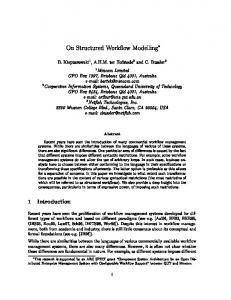
1.3 OUTLINE OF THE THESIS The general structure of this work is presented in Fig. 1.1. It is built on four journal papers (one is still in revision) and one presentation from an international conference. These five key publications are complemented with three additional supporting publications (see Table 1.1). The supporting publications are not directly integrated in this work, yet they represent preliminary work that was essential to achieve this dissertation. To increase the uniformity of this dissertation, the remaining chapters are written in a manuscript style as well. At the beginning of each chapter a short overview is presented that situates the chapter in the dissertation and describes its link with the key and supporting publications. A complete overview of all publications is listed in Appendix P1.

Fig. 1.1 Research structure. The links with the key publications are between brackets.

The first two chapters define the problem statement. Chapter 1 provides insight into the general context of this work and defines the objectives and the research questions. Chapter 2 presents the current state-of-the-art of LCA in the construction sector and consequential modelling, and includes a more detailed definition of the knowledge gaps addressed in this work. Afterwards, two explorative case studies are presented in Chapter 3. The first exploratory case study focusses on an assessment at a building level. Differences between an attributional and a consequential approach and also the practical limitations and research opportunities of both approaches are examined. Taking into account the identified research opportunities, the second explorative case study is about the Belgian electricity grid mix and presents an early version of the general method as presented in Chapter 4. The experience gained during this process enabled the further optimisation of the method by making it more consistent. Based on the insights gained in the first two parts, a method for the identification of marginal suppliers is presented in Chapter 4. It has a particular focus on the definition of Chapter 1. Introduction | 7

geographical market boundaries and the identification of the most sensitive suppliers. In addition to the general method three additional sensitivity scenarios are included in this chapter as well. Chapter 5 contains two case studies. The first case mainly focuses on testing and validating the improved method. The second case leaves the pure testing behind and proceeds with assessing the potential burdens and benefits of demountable and reusable walls. The chapter ends with a general discussion about the proposed method and the practical issues encountered during its application. Chapter 6 summarises the main results of this work. It provides recommendations and some suggestions for future research efforts. Finally, more detailed information about the data collection, assumptions and results is provided in the printed appendices at the end of this work. Extra information such as datasets, calculation files and scripts are available in a digital appendix 3.

Key publications J1

M. Buyle, J. Braet, A. Audenaert, Life cycle assessment in the construction sector: A review. Renewable & Sustainable Energy Reviews. 26, 379–388 (2013)

J2

M. Buyle, J. Braet, A. Audenaert, W. Debacker, Strategies for optimizing the environmental profile of dwellings in a Belgian context: A consequential versus an attributional approach. Journal of Cleaner Production. 173, 235–244 (2018)

J3

M. Buyle, M. Pizzol, A. Audenaert, Identifying marginal suppliers of construction materials: consistent modeling and sensitivity analysis on a Belgian case. The International Journal of Life Cycle Assessment., 1–17 (2017)

J4

M. Buyle, J. Anthonissen, W. Van den bergh, J. Braet, A. Audenaert, Analysis of the Belgian electricity mix used in environmental life cycle assessment studies: how reliable is the ecoinvent 3 mix? (under revision)

C1

M. Buyle, M. Pizzol, A. Audenaert, Defining geographical market boundaries of construction materials: a sensitivity analysis of modelling assumptions, Abstract from 23rd SETAC Europe LCA Case Studies Symposium, Barcelona, Spain (2017)

Supporting publications J5

M. Buyle, A. Audenaert, J. Braet, W. Debacker, Towards a More Sustainable Building Stock: Optimizing a Flemish Dwelling Using a Life Cycle Approach. Buildings. 5, 424–448 (2015)

C2

M. Buyle, J. Braet, A. Audenaert, Life Cycle Assessment of an Apartment Building: Comparison of an Attributional and Consequential Approach. Energy Procedia. 62, 132–140 (2014)

C3

M. Buyle, J. Braet, A. Audenaert, The application of survival analysis for service life prediction of building materials: a proof of concept. In 14th International Conference on Durability of Building Materials and Components: 29-31 May, 2017, Ghent, Belgium, 1–9 (2017)

Table 1.1 Publications included in this work. J = Peer-reviewed journal paper, C = Conference proceeding

3

Retrievable at: https://www.uantwerpen.be/nl/personeel/matthias-buyle/mijn-website/

8|

2 2 FROM BUILDING TO SUSTAINABLE BUILDING “I don't know how to read but I've got a lot of toys” Bad religion

After the general introductory Chapter 1, which defines the objectives and research questions, Chapter 2 is the second chapter that describes and delimits the problem statement of this work. This chapter contains a literature review of consequential LCA in the construction sector. The information provided by this review yields the essential building blocks for the development of the method in the following chapters. This chapter is subdivided in three parts. The first part (Section 2.1) focuses on LCA in the construction sector, mainly targeting research at building level. This part was published in 2013 (key publication J1) and no changes were made compared to the published version. This study is slightly outdated, as the most recent included studies date from 2012. So in the second part (Section 2.2), an update on LCA in the construction sector is presented Chapter 2. From building to sustainable building | 9

including more recent research. The objective of Section 2.2 is not to present a comprehensive literature review for this period, but to assess to what extent the observations of the first part are still valid and to identify new evolutions and trends. The last part (Section 2.3) addresses the current state-of-the-art in consequential modelling, without specifically targeting the construction sector. A comparison between attributional and consequential LCA is included as well. This section ends with a more detailed review on the process of the identification of marginal suppliers. Parts of this last part were published in key publication J3. Parts of this chapter were presented in the following publications:  

M. Buyle, J. Braet, A. Audenaert, Life cycle assessment in the construction sector: A review. Renewable & Sustainable Energy Reviews. 26, 379–388 (2013) M. Buyle, M. Pizzol, A. Audenaert, Identifying marginal suppliers of construction materials: consistent modeling and sensitivity analysis on a Belgian case. The International Journal of Life Cycle Assessment., 1–17 (2017)

2.1 LCA IN THE CONSTRUCTION SECTOR (UNTIL 2012) 2.1.1

INTRODUCTION

In our society buildings are omnipresent, but inevitably they entail negative consequences from an environmental point of view. During their life span, they consume plenty of resources and energy, occupy land and eventually they are demolished. As the interest in environmental issues is rapidly growing, also within the construction industry, more attention is being paid to sustainable housing technologies and construction methods. This general increasing awareness led to the Kyoto-protocol, an international agreement on reducing the emission of greenhouse gasses and global warming [36]. In the construction sector, this resulted for instance in regulations to decrease energy consumption of dwellings and consequently their ecological burdens i.e., the Energy Performance of Buildings Directive 2002/91/EC (EPBD, 2003) and the revised EPBD 2010/31/EU issued by the European Union [4,5]. Such regulations make sense as for example in Flanders households have a share 36–40% of the total energy consumption, and the residential sector in Belgium produces about 40% of the emitted CO2 [14,15]. The European regulations stimulated the emergence of new building concepts such as low-energy and even self-sufficient houses [37,38]. When only focusing on energy consumption, lowenergy houses excel compared to standard houses [39]. But besides energy consumption, also other aspects affect the sustainability of buildings, a concept that covers ecological, economic and social aspects. With the increasing awareness of these issues, plenty of tools have been developed to asses sustainability from different viewpoints and for a variety of users [40]. Some examples are Environmental Impact Assessment (EIA), System of Economic and Environmental Accounting (SEEA), Environmental Auditing and Material Flow Analysis (MFA). In addition, several methods have been developed specifically for the construction sector such as BREEAM and LEED, 10 |

which provide measurement ratings for (green) buildings. A discussion of all these tools is beyond the scope of this review that will focus on life cycle assessment (LCA), because this is commonly used and much more detailed compared to rating tools. LCA is a tool to investigate environmental burdens of a product or process, considering the whole life cycle, from cradle to grave [27]. All aspects considering natural environment, human health and resource depletion are taken into account and together with the life cycle perspective, LCA avoids problem-shifting between different life cycle stages, between regions and between environmental problems.

2.1.2

A BRIEF HISTORY

The first studies on environmental impacts date from the 1960s and 1970s, focusing on the evaluation or comparison of consumer goods, with only a small contribution to the use phase [41]. According to Guinée et al. one of the first (unpublished) studies was executed by Midwest Research Institute (MRI) for The Coca Cola Company in 1969, including resources, emission loadings and waste flows for different beverage containers [41]. In the beginning of the 1980s, life cycle thinking appears in the construction sector with a study of Bekker, with focus on the use of (renewable) resources [42]. These early researches applied diverging methods, approaches, terminologies and results. There was a clear lack of scientific discussion and consensus and the technique was often used for market claims with doubtful results, which prevented LCA from becoming a generally accepted and applied analytical tool [43]. In the 1990s came a period of standardisation, with the organization of workshops and the publication of several hand-books and scientific papers [43–48]. From this decade, the Society of Environmental Toxicology and Chemistry (SETAC) started playing a leading and coordinating role by bringing the LCA practitioners together and harmonizing the framework, methodology and terminology, which resulted in the SETAC ‘Code of Practice’ [49]. From 1994 the International Organization for Standardization (ISO) was involved as well, whose main achievement has been the harmonization of methods and procedures, resulting in the ISO 14040 standard series, first published in 1997 [50]. The result of this standardisation was the creation of a general methodological framework, which made it easier to compare different LCAs. It is important to keep in mind that even with the consensus on the framework, ISO never aimed at defining the exact methods by stating ‘there is no single method for conducting LCA’ [27] . From the start of the 21st century, interest in LCA has been increasing rapidly, as can be seen in the overview of case studies in Table 2.1. Life cycle thinking is also growing in importance within European Policy as, i.e. demonstrated by the Communication from the European Commission on Integrated Product Policy (IPP) [51]. A direct result of the IPP is the development of the International Reference Life Cycle Data System Handbook (ILCD), a practical guide for LCA according to the current best practice published in 2010, complementary with the ISO 14040 series [52–54].To facilitate the use of LCA and to improve supporting tools and data quality, the United Nations Environment Program (UNEP) and SETAC launched the Life Cycle Initiative [55,56]. Another indication of the Chapter 2. From building to sustainable building | 11

growing importance of life cycle thinking is the emergence of Environmental Product Declarations (EPDs) [57,58]. An EPD is a set of quantified environmental data for a product with pre-set categories of parameters based on the LCA standards (ISO 14040 series) and additional environmental information is not excluded. This system makes it easier for designers to choose for eco-friendly products or materials [59]. In the last decade, there have been also some developments specifically targeting the construction sector, in addition to the ISO 14040 standards. In 2003, SETAC published a state-of-the-art report on Life-Cycle Assessment in Building and Construction, an outcome of the Life Cycle Initiative [60]. This study highlights the differences between the general approach of LCA and LCAs of buildings. Such standardisation continued, with two leading organizations, the International Organization for Standardization (ISO) and the European Committee for Standardization (CEN). The first, more specifically the ISO Technical committee (TC) 59 ‘Building Construction’ and its subcommittee (SC) 17 ‘Sustainability in Building construction’, published four standards describing a framework for investigating sustainability of buildings and the implementation of EPDs [61]. The CEN Technical Committee (TC) 350 ‘Sustainability of construction works’ is developing standards for assessing all three aspects of sustainability (economic, environmental, social) both for new and existing construction works and for facilitating the integration of EPDs of construction products [62]. Since these standards are very recent, only very few studies have been executed according to them.

2.1.3

LCA METHODOLOGY

As described in the previous section, in current practice LCAs are executed according to the framework of the ISO 14040 series [27]. To analyse the environmental burdens of processes and products during their entire life cycle, four steps have to be run through, making it possible to compare different studies: goal and scope, Life Cycle Inventory (LCI), Life Cycle Impact Assessment (LCIA) and interpretation [31,63–65]. The first step, goal and scope, defines purpose, objectives, functional unit and system boundaries. One of the strengths of LCA is defining investigated products and processes based on their function instead of on their specific physical characteristics. This way, products can be compared that are inherently different, but fulfil a similar function e.g., paper towels versus reusable cotton towels for drying hands. The second step (LCI) consists of collecting, as well as describing and verifying, all data regarding inputs, processes, emissions, etc. of the whole life cycle. Third (LCIA), environmental impacts and used resources are quantified, based on the inventory analysis. This step contains three mandatory parts: selection of impact categories depending on the parameters of goal and scope, assignment of LCI results to the selected impact categories (classification) and calculation of category indicators (characterization). In the current practice there is a large set of impact categories commonly used, for example global warming potential (GWP), but ISO 14044 states that when the existing categories are not sufficient, new ones can be defined [31]. The LCIA step also contains two optional steps: normalization and weighting. Normalization is the calculation of the magnitude of category indicator results relative to 12 |

some reference information, for example the average environmental impact of a European citizen in one year. Weighting is the process of converting indicator results of different impact categories into more global issues of concern or a single score, by using numerical factors based on value-choices, for example based on policy targets, monetarisation or panel weighting—the authors emphasize the fact that this is the first and major step in an LCA where non-objective measures come in. This is part of the environmental mechanism (see further). The fourth and final step is the interpretation of the results [27,31]. The approaches to calculate environmental impacts can be subdivided into two types, attributional and consequential LCA. Attributional LCA is defined by its focus on describing the environmentally relevant flows within the chosen temporal window, while consequential LCA aims to describe how environmentally relevant flows will change in response to possible decisions [32,66]. Generally, most authors state that consequential LCAs are more appropriate for decision-making, unless their uncertainties in the modelling outweigh the insights gained from it [67,68]. When LCA is used to indicate hotspots of the environmental burdens as base for improvements, the consequences of these implementations should not be neglected. Such actions will influence the production of upstream products, other life cycles and more in general, other economic activities. Both positive and negative mechanisms can occur. If efficiency measures are profitable, economic activities may increase and diminish the environmental benefits. This negative mechanism is also called a rebound effect [69]. A positive mechanism is that investments in emerging technologies are likely to reduce manufacturing costs, which can trigger similar investments of other manufacturers [66]. If such a new technology has a lower impact, this can entail huge savings for the entire society and in that case a consequential approach is more appropriate. Although ISO standards describe the global framework of an LCA, the exact technique to calculate environmental impacts is not defined. Depending on the nature of research, different methods can be chosen, defined by their environmental mechanisms as described in ISO 14044 (see Fig. 2.1). Such a mechanism is the process for any given impact category, linking the LCI results to category indicators i.e., a sequence of effects that can cause a certain level of damage to the environment. These category indicators can be combined to more comprehensible and general indicators. Environmental mechanisms consist of sequences of complex conversion processes and the valuation factors used in environmental mechanisms are the main difference between LCA methods, as they may assign a different importance to the same physical values. To quantify environmental impacts two approaches can be identified, namely the problemoriented (midpoints) and damage-oriented (endpoints) ones, which can be combined as well [70]. The first group of methods uses values at the beginning or middle of the environmental mechanism. Impacts are classified on environmental themes such as global warming potential, acidification potential, ozone depletion potential, etc. This type of method generates a more complete picture of the environmental impacts, although the problem of incomparability may arise: is it worse to have 2 kg CO2 eq. or 1 kg SO2 eq.? Still these midpoints are important as they are directly linked to physical characteristics. The

Chapter 2. From building to sustainable building | 13

Fig. 2.1 Schematic presentation of an environmental mechanism underlying the modelling of impacts and damages in Life Cycle Impact Assessment (ISO 14044: 2006) [31]

second group is at the end of the mechanism, where the midpoints are grouped into general damage categories such as human health, natural environment and resources, which eventually can be calculated into a single score. The results of the latter are easier to understand, but tend to be less transparent [71,72]. Another drawback of the endpoint approach is the use of more subjective factors in the conversion to general categories. This will entail greater uncertainties and affect the reliability of the results. A weakness in current practice of LCA is that different methods applied to an identical case can generate different results, e.g. a narrow scope carbon footprint study versus studies with a set of more differentiated impact indicators [72,73]. Various methods can assign a different importance to properties or impacts, which can result in other suggestions of action to reduce the environmental burdens [74]. Results of an LCA are no absolute values and therefore cannot serve as a certification on itself. They do not guarantee the sustainability of a product or service, but are valuable for the comparison of different products and processes. Comparing results of an LCA is only meaningful when the subjects fulfil exactly the same function in accordance with their goal and scope definitions. Another weakness is the inability to investigate local impacts as, in general, environmental damage is calculated on global scale. In reality such assumptions are not always valid and emissions, for instance, can have a greater impact when they are released in vulnerable areas. A better solution is to combine LCA with tools that are developed to assess local impacts, like Risk Assessment [40]. Additionally, local emissions can have also other consequences i.e., affect the indoor climate of a dwelling. From an environmental point of view, such emissions may deliver no significant contribution, but to ensure a healthy indoor climate within an LCA or other local damage, extra criteria should be integrated in the functional unit, often in order to comply with regulations [75]. This shows once again the difficulty and importance to incorporate qualitative requirements into LCA.

14 |

2.1.4 2.1.4.1

DEVELOPMENTS IN THE CONSTRUCTION SECTOR Academic research

In industrial processes, LCA is widely spread and it is used frequently to evaluate the environmental impact of products and processes [76]. Buildings however are special products that differ thoroughly from these mostly controlled processes. In the construction industry, such a study is therefore on the average much more complex because of multiple issues: the long life span of the entire building (50–100 years [77–79]) and consequently a lower predictability of uncertain variables and parameters (1), a shorter life span of some elements and components (2), the use of many different materials and processes (3), the unique character of each building (4), the varying distances to factories e.g., Canadian wood used in Belgian dwellings (5), the evolution of functions over time because of maintenance and retrofitting (6), etc. [70,78,80,81]. The long life span and dependence of user behaviour thus require much more assumptions, coming with larger uncertainties and consequently influence the credibility of the results [17]. So since the building process is less standardised than industrial processes, such a life cycle assessment is a challenging task. A classification of existing studies could be done according to the magnitude of the subjects, going from materials to building components and finally the analysis of entire buildings [70]. Discussing the analysis of materials and components is beyond the scope of this review, however such studies have proved their value. When applying results of such studies, some things have to be kept in mind. First, when comparing materials two possible alternatives have to fulfil the exact same function e.g., bricks and wood do not have the same structural characteristics. Studies on components, on the other hand, can partly counter this problem by incorporating additional requirements in their functional unit e.g., a cavity wall has to meet legal thermal or structural demands. Such studies are often useful during the design process, as at this stage many decisions are made about structural concepts and used materials, and they are strongly linked to the European policy e.g., the Integrated Product Policy, with tools as EPDs and Ecodesign [70]. In this paper, the main focus lies on LCAs of entire buildings. This way the contribution to the total impact of different products, processes and life cycle stages becomes more clear and environmental hotspots can be identified. The results reveal more about building concepts in general and less about the chosen materials. In these cases, the entire building is the functional unit, but with great differences in building properties, size, location, impact methods, etc. Therefore results are not directly comparable, but still trends can be identified. Table 2.1 contains an overview of published academic studies of LCAs of whole buildings and their main characteristics. A lot of these studies are simplified LCAs only discussing energy, especially the early studies. They are also known as a Life Cycle Energy Assessment (LCEA) and consider the cumulative energy demand during the different phases of the life cycle: embodied (production and construction), operational, demolition and recycling energy [82]. As stated by Huberman and Pearlmutter, this method is a single score indicator. Therefore the same remarks can be made as for the endpoint methods:

Chapter 2. From building to sustainable building | 15

16 |

1997

2001

2010

2003

2007

2012

1998

2009

2009

2001

2007

1996

2009

2009

2005

2000

2007

2011

2008

2004

Adalberth [18]

Adalberth et al. [102]

Allacker [113]

Arena and Rosa [360]

Asif et al. [212]

Audenaert et al. [361]

Blanchard and Reppe [114]

Blengini and Di Carlo [71]

Blengini [96]

Chen and Burnett [109]

Citherlet and Defaux [93]

Cole and Kernan [107]

De Meester et al. [85]

Dewulf et al. [86]

Erlandsson and Levin [99]

Fay et al. [362]

Gerilla et al. [106]

Guardigli et al. [111]

Huberman and Pearlmutter [83]

Junnila [363]

Finland

Israel

Italy

Japan

Australia

Sweden

Belgium

Belgium

Canada

Switzerland

China

Italy

Italy

USA

Belgium

Scotland

Argentina

Belgium

Sweden

Sweden

Country

1

1

2

2

2

1

1

65

12

3

2

1

2

2

1

1

2

16

4

3

Cases

O

R

R

R

R

R

R

R

O

R

R

R

R

R

R

R

S

R

R

R

Type Build.

LCA

LCEA

LCA

LCA

LCEA

LCA

LCEA

LCEA

LCEA

LCA

LCEA

LCA

LCA

LCEA

LCA

LCEA

scr. LCA

LCA

scr. LCA

LCEA

Type

Midpoints

Cum. En. + GWP

Cum. En. Midpoints + External costs Eco-Ind.99

BYKR

Cum. Exergy

Cum. Exergy

Cum. En.

CML 2

Cum. En.. + GWP Midpoints + Eco-Ind.99 + EF + EPS2000 Midpoints + Eco-Ind.99 Cum. En.

Eco-Ind.99

Cum. En.

50

50

?

35

100

35

50

75

50

?

40

40

70

50

?

?

50

60

External Costs Midpoints (SBID)

50

50

Cum. En. Midpoints (SBID)

Life span

Impact Method

x

x

x

x

x

x

-

x

x

x

x

x

x

x

x

x

x

x

x

x

Prod.

x

x

-

x

x

x

-

x

x

x

-

x

x

x

x

-

x

x

x

x

Use

x

-

-

x

-

-

x

x

x

x

x

x

x

x

x

-

-

x

x

x

EoL

-

-

-

x

x

-

x

-

x

x

-

x

-

x

-

-

-

x

x

-

Sens.

x

x

x

x

x

-

x

x

?

x

x

x

x

x

-

-

x

x

x

x

Transp.

Table 2.1. Overview case studies

R = Residential, O = Office, S = School, x = Included, - = Excluded, ? = Unknown, Cum. En. = Cumulated Energy, EF = Ecological Footprint, GWP = Global Warming Potential, BYKR = Swedish Building Eco-Cycle Council

Year

Author

Chapter 2. From building to sustainable building | 17

2008

2006

2004 2009

2010

2001

2003 2012 2012 2003 1998

2000

2002 2006 1999 2011 2008

2005

Kofoworola and Gheewala [19]

Marceau and VanGeem [108]

Mithraratne and Vale [105] Ortiz et al. [92]

Ortiz et al. [103]

Peuportier [75]

Reddy and Jagadish [364] Rosa and Aqisa [104] Rossi et al. [365] Scheuer et al. [366] Suzuki and Oka [367]

Thormark [73]

Thormark [94] Thormark [95] Winther and Hestnes Wu et al. [368] Xing et al.[369]

Zimmermann et al. [370] Switzerland

Sweden Sweden Norway China China

Sweden

India UK Belgium USA Japan

France

New Zeeland Spain Spain Colombia

USA

Thailand

Country

-

1 1 5 1 2

2

3 3 2 1 10

3

2

3 1

2

1

Cases

All

R R R O O

R

R R R S O

R

R

R R

R

O

Type Build.

LCA

LCEA LCEA LCEA LCEA LCA

LCA

LCEA LCA LCEA LCA LCEA

LCA

LCA

LCEA LCA

LCA

LCA

Type

CML 1 (+ extra indicators) Cum. En. CML 2 Cum. En. + GWP Midpoints + Cum. En. Cum. En. + GWP Eco.Scar.1990 + EPS1992 + ET1992 Cum. En. Cum. En. Cum. En. Cum. En. + CO2 Midpoints Eco.Scarc.1990 + GWP + 2000 W soc.

CML 2

Midpoints Eco-Ind.99 + EDIP96 + EPS2000 Cum. En. CML 2

Impact Method

?

50 50 50 50 50

?

? 50 50 75 40

80

50

100 50

100

50

Life span

x

x x x x x

x

x x x x x

x

x

x x

x

x

Prod.

x

x x x x x

-

x x x x

x

x

x x

x

x

Use

-

x x x ?

x

x x x -

x

x

x -

-

x

EoL

-

x x -

x

x -

x

x

x

x

-

Sens.

x

x x x x -

x

x x x x -

x

x

x x

x

x

Transp.

Swedish Building Eco-Cycle Council

Table 2.1. Overview case studies (continued)

R = Residential, O = Office, S = School, x = Included, - = Excluded, ? = Unknown, Cum. En. = Cumulated Energy, EF = Ecological Footprint, GWP = Global Warming Potential, BYKR =

Year

Author

it is easier to draw conclusions, but the results are much more subjective and less reliable [83,84]. A variation on this method is Life Cycle Exergy Assessment, developed by De Meester and Dewulf, which takes the quality of the energy into account [85,86]. Exergy is the work potential of an amount of energy with respect to its environmental conditions [87]. According to this method, the conversion of high grade energy (electricity) into low grade energy (heat) should be highly discouraged. Less frequent are the LCAs considering also other impact categories, which sometimes take the entire life cycle into account, but often only some life cycle stages. A wide variety of impact methods is used, from midpoint to endpoint (e.g. CML, Eco-indicator 99, Carbon footprint), sometimes a set of different methods is applied or results are examined whether they comply with policy targets. A detailed discussion on these impact methods is beyond the scope of this review, nevertheless in Table 2.1 the applied impact method is represented for each of the studies (an overview can be found in [88]). As cited in Section 2.1.3, from a methodological point of view, a subdivision can be made between damage- and problem-oriented methods. In practice however, as can be seen at the presented studies, there appears to be a more complex variety, where the wide range of generally accepted methods sometimes are combined with specifically developed variants. The most basic studies are the ones using only midpoint results directly related to impact categories, without any grouping nor weighting however as mentioned before, they are also the most objective (1). Next are the analyses calculating a selection of possible impacts of a life cycle e.g., the cumulative energy or exergy demand and carbon footprints (2), as discussed before. A third group comprises the distance-to-target-methods evaluating sustainability related to fixed or legal policy targets (3) e.g., BYKR and Ecological Scarcity 2006. Some other methods are strongly simplified and thus have to be interpreted with care, especially if they are widely spread (4) e.g., Ecolizer 2.0. The more commonly used and generally accepted methods are the damage-oriented ones (5) e.g., Eco-Indicator 99, EPS, EDIP, external costs, and the problem oriented (6), e.g. CML 2001. Finally, one of the newer methods is Recipe, combining both the midpoint and the endpoint level and based on Eco-Indicator 99 and CML-IA (7); yet, it has not been utilized within the present review [88–90]. Before looking at the results of the studies, some remarks must be made, since the characteristics of the cases differ sometimes substantially. First, not all studies have the same coverage of the life cycle. The following aspects are sometimes excluded: transport, waste treatment, maintenance, water use, etc. Also the accuracy differs i.e., some studies are coarse and not as detailed which only take the most obvious products and processes into account; therefore a distinction can be made between detailed LCAs and screening LCAs as well, not based on methods, but on the level of detail. Next, there is a wide variety in the methods used. Fourth, various topics were subject of research. Most of the studies consider residential buildings, but schools and office buildings have been investigated as well. The cases differ in construction period, level of technology or building concept. Finally, not always all phases of the life cycle have been included. In addition, some extra steps can be included besides the mandatory steps of an LCA, namely a sensitivity check and an uncertainty analysis. The first one is to verify the sensitivity of significant data elements of the results by varying parameters, choice of data, 18 |

assumptions or impact assessment methods to check if the results are still valid. If not, this has to be documented. Another optional step is to investigate uncertainties of the life cycle inventory which can be divided into different categories: variability and stochastic error of the figures which describe the inputs and outputs due to e.g., measurement uncertainties, pro-cess specific variations, temporal variations, etc. (1), appropriateness of the data (2), model uncertainty e.g., due to inappropriate descriptions of processes (3) and finally neglecting the important flows (4) [91]. Uncertainties related to deviations of the first category are inherent to every practical process and data quality indicators are sufficiently available, for example in the Ecoinvent database; however only the study of Blengini and Di Carlo included this step [71]. As mentioned before, the parameters of the existing research vary substantially, but nevertheless some common trends can be indicated. One of the conclusions of almost every research is the dominance of the use phase, especially due to energy consumption of heating and cooling. The share of the use phase of standard houses is in the range of 60– 90% of the total environmental burdens, mainly with a contribution to global warming potential [18,19]. Even in very different climates this conclusion appears to be valid, as studies in Nordic and Mediterranean countries come to similar results [18,92]. A common conclusion of these studies is therefore the necessity of reducing the need for heating and/or cooling by improving insulation, improving air-tightness and controlling ventilation. Some of these aspects can be found in the European Policy, which is strongly focused on reducing energy consumption [4]. The conclusions mentioned in the previous paragraph are generally taken into account during the design and execution of low-energy houses whereby the energy use can strongly be reduced. Several studies of this kind of buildings have been carried out which often also analyse the impact of optimisation suggestions, however only on dwellings so far. Blengini and Di Carlo investigated a low energy dwelling in Italy. Although the energy consumption was ten times lower than the reference standard house, the total environmental impact was only reduced by a factor 2.1 [71]. So when the energy use is pushed back, the other phases of the life cycle are growing in relative importance, like for example construction methodology, the choice of materials and end-of-life scenarios. Huberman reaches similar conclusions: if operational energy (use) decreases, embodied energy (materials) increases relatively, a trend which occurs more often since industrialization [83]. Citherlet and Defaux mention that it is only relevant to pay much attention to the impact of the production and end-of-life phase (referred to as ‘indirect impacts’) when the yearly energy consumption is below 150 MJ/m² [93]. As new buildings are designed more energy-efficiently, a next step in research is to pay more attention to the growing relevance of the other phases. Thormark focused on the recycling potential and the concept ‘Design for disassembly’, while Blengini examined the demolition of a flat to verify and/or complete the literature data [73,94–96]. Both studies show the benefits of reuse in the first place, which is slightly superior to recycling, yet they do have reservations about the feasibility of reuse on a large scale since it requires major changes from current practice and may not be profitable. Goverse et al. describe problems of a switch-over of existing economic structures, especially in this case, where large Chapter 2. From building to sustainable building | 19

changes in technical and network dimensions are necessary [97]. In line is the research of Erlandsson and Levin focusing on the benefits of refurbishment, a construction method that is gaining importance as can be seen in Belgian statistics: the share of building permits for renovations increased with more than 30% over the last 15 years [98]. Refurbishment is generally more eco-friendly, but urban regulations are a limitation that often do not allow all optimal measures, especially if they occur on the outside of the building, for example additional insulation [99]. Complementary to the previous paragraph is the static and inflexible approach of the calculation of the use phase of most studies. In the best case, and the most common, replacements of components are included after the predicted technical life span by the same components. In reality however, they are more likely to be replaced by technologically more advanced components with a better performance. In addition, during the life span of a building, more radical renovations will often be carried out to meet current (or future) comfort demands [99,100]. These aspects influence the use phase, particularly when they improve the energetic performance and therefore they should be included. However LCA is a static tool, this drawback can be overcome by including scenarios, as described in the study of Van Nunen [100]. In this study different scenarios for renovation cycles have been developed and they provide a better understanding of the importance of maintenance and refurbishments. Such an approach is also useful to indicate priorities for renovating a building, as described in the study of Verbeeck and Hens, which compares i.e., scenarios for optimising new buildings with scenarios for renovations [101]. The international nature of research on LCA in combination with local production chains makes the comparison more difficult. The regional electricity mix, for instance, has a great influence on the impact of the use phase [102]. The study of Ortiz-Rodríguez et al. compares a dwelling in Spain with one in Colombia [103]. In this study, 20% of the total required energy is covered by electricity, of which the production differs significantly between the two countries. The environmental burden of electricity production is twice as large in Spain as in Colombia for most of the impact categories, mainly due to the larger share of hydropower. Another example is the study of Braet, that compares container pipeline transport versus road transport [76]. As sensitivity analysis, different scenarios for electricity production are included and they have a great effect on the results, also strongly related to impact assessment methods. In the coal energy scenario the road concept performs better than the pipeline concept using the ReCiPe or IPCC GWP 100a method. In the natural gas scenario both concepts have an equal environmental impact for all available methods used. In all other electricity production scenarios, such as nuclear energy, the pipeline concepts outperforms the road concept for all available impact assessment methods used. Cuéllar-Franca and Azapagic investigate also the influence of the choice of functional unit, which is in most studies the entire building or net habitable floor area [104]. This study however compares three dwelling type alternatives (detached, semi-detached and terraced), each with their typical size and characteristics. The number of inhabitants is assumed to be the average UK household size, consisting of 2,3 people. When looking to the impact per square meter as functional unit, the detached house has the lowest impacts 20 |

per unit of floor area. This is mainly due to the impacts related to the household size, such as water consumption, energy for cooking, etc. which is the same for all three dwelling type alternatives. When looking at impact per inhabitant however, the smallest and most compact alternative (terraced) has the lowest impact. Not only energetic but also structural concepts have been compared, mainly renewable (wood) versus non-renewable materials (masonry, concrete, steel) in the context of lowenergy dwellings. Most research assigns better results to wooden structures [105–107]. Wood is easier to manipulate and CO2 neutral, while production of steel and concrete induces more burdens due to production and processing and has a higher embodied energy. However, the use of timber frames is limited to buildings up to three floors [107]. Only the research of Marceau and VanGeem comes to opposite conclusions, with a preference for concrete structures, mainly because of the higher land use of wood [108]. Another frequent conclusion is the minor importance of the transportation of materials during construction. Almost all the research included this aspect, but as building materials are often locally produced, the travel distances and associated impacts are limited, for example 1% or less according to Adalberth and Ortiz et al. [18,92]. Even when some parts are transported over a long distance, the associated impact does not play a major role. Designers and public administrators participating in the Italian study by Blengini and Di Carlo on a low energy house were surprised by the minor contribution of transportation, as it was feared that triple glazed windows imported from Germany and cork slab transported over long distances by truck and ship would compromise the environmental performances [71]. Only when almost all materials are transported over a great distance, transportation becomes an issue of concern, which can be seen in the research of Chen et al. Materials of two analysed office buildings in Hong Kong are mostly imported, often overseas, which can be seen in the contribution of transportation of 7% to the total environmental burdens [109]. 2.1.4.2

Regulatory developments

The previous sections demonstrate that in current academic practice, only general trends can be derived from the examined studies. However buildings are not directly comparable. All these studies are executed according to the framework described in the ISO 14040 series, which is applicable to all types of studies. As life-cycle thinking becomes more integrated in policy and marketing, there will be a need for a more delineated framework, specifically for buildings. As mentioned in Section 2.1.2, international organizations like ISO and CEN are working on the standardisation of LCAs in the construction sector in order to improve the comparability of such studies. A main goal of the latter is documenting the environmental performance of a building for use in e.g., declaring environmental performance, labelling and marketing. As stated by CEN TC 350 in EN 15978:2011, ‘the purpose of this European Standard is to provide calculation rules for the assessment of the environmental performance of new and existing buildings’ [110]. These rules consist in the description of functional equivalent, system boundaries, procedures to be used for the inventory analysis, a list of environmental indicators and procedures for the calculation of the impact categories, rules for reporting and communicating results, etc. This framework

Chapter 2. From building to sustainable building | 21

is very similar to the one of EPDs, which encourages and facilitates the incorporation of results of external studies. The previously mentioned regulation is part of a larger set of standards, also focusing on other aspects of sustainability like social and economic performance, both at the building and product level. Such rules for standardisation can be a limitation as well, by excluding environmental indicators which are integrated in commonly used impact methods. For example the successor of Eco-indicator 99, ReCiPe, that combines midpoints and endpoints, takes land use into account, an impact category that is excluded in the new standards [89,110]. Since this is a popular series of methods, many (existing) studies are therefore not in line with the new standards. The exclusion of land use can affect results significantly, especially if a lot of wood is used e.g., when comparing timber frame with heavyweight constructions. Guardigli et al. investigated a wood structure in Italy and states the main environmental impact is due to the land use of wood [111]. A possible solution is to follow the new standards, but supplement them with other relevant impact categories.

2.1.5

DISCUSSION AND LIMITATIONS

This review focuses on case based LCA studies of entire buildings, being a great tool to investigate building concepts and to support decision-making to reduce environmental burdens. Nevertheless the LCA methodology has some inherent limitations, consequently results should be interpreted and used with care. First, the cases are difficult to compare because of their specific properties like lay-out, climate, comfort requirements, local regulations, etc. The widespread estimations of the life span of buildings is a second limitation. These two limitations can be partly overcome by calculating the annual burdens per square meter useful floor surface or per person, still other aspects of the studies can differ e.g., system boundaries, assumptions, level of detail, LCIA methods, etc. Next, LCA is merely a model and simplification of reality, so assumptions have to be made that can generate uncertainties on different levels: model, scenario and parameter uncertainties [112]. The first two aspects are difficult to process statistically and are often excluded, but with the latter this is possible as data quality indicators are available for all materials and processes in the ecoinvent database (see also Section 2.1.4). Parameter uncertainty is also often enhanced by data gaps, resulting in less accurate data to be used. When considering the variability and stochastic error of the figures, the reliability is enhanced but the interpretation has to be performed by using probability statements, which are less common but still useful conclusions can be drawn. As mentioned before, the use phase of buildings is the dominant factor of the environmental burdens over the entire life cycle, especially through the high energy consumption. The burdens of this phase are based on estimations, taking average values of the whole society into account. Since individual inhabitant behaviour is difficult to predict, it is also an issue of concern when considering the reliability of any conclusion on energy consumption. This limits the practical importance of LCA, no matter how accurate calculations may have been carried out. Research concluded that many efficiency improvements do not reduce energy consumption as much as predicted. As they make 22 |

energy services cheaper, the demand for these services will increase. For example, if a dwelling is well insulated, residents are more likely to heat up the spaces above the calculated temperature, since this entails only a limited additional cost. This psychological phenomena is called the rebound effect and until now this has not been taken into account [69]. A stochastic approach based on real data could partly counter this problem; however, rebound effects will always occur as economic savings will trigger other (non-building related) expenditures which of course entail also environmental burdens. An extra difficulty is the fact that user behaviour and consumption habits are often regionally defined, as investigated by Ortiz-Rodríguez et al. The difference in environmental impact between a Spanish and Columbian dwelling is partly caused by such social differences [103]. Another drawback of current LCA practice within the construction sector is the isolated approach of environmental issues. Often the focus is limited to the search for environmental optima, but without linking it to other aspects. For example, LCA does not take into account any quality, energetic, structural nor aesthetic requirements. According to Allacker, the design plays a major role in the environmental profile, but this has been barely investigated yet [113]. Also financial feasibility is hardly ever taken into account, although ready-to-use tools are available, for example Life Cycle Costing. Only a few researchers include financial and ecological aspects and give a more complete picture, like Allacker, Blanchard and Reppe, and Verbeeck [101,113,114]. Although new regulations and frameworks have been worked out for assessing all aspects of sustainability, at the moment they are not frequently implemented.

2.1.6

RESEARCH OPPORTUNITIES

The growing importance of LCA as a scientific tool to evaluate environmental burdens is a positive trend; however there are still many research opportunities and areas to improve current practice. The construction sector causes unwanted environmental effects, but economic costs to repair or avoid them rarely appear in the resulting prices of goods and services. Internalization is nevertheless crucial if our society wishes to enhance its sustainability on the long term, without burdening future generations. As this is currently not occurring systematically, it is a challenge to reflect environmental costs of building materials and processes in their sales prices. This way manufacturers or service providers should be held responsible to repair or counter the environmental effects of their production processes. The link between environmental impact and cost implications needs to be established and clearly communicated. Currently the main focus is at energy reduction, both in policy and research. However, the research of Allacker states that other aspects may play an important role too, like water consumption. The impact of water consumption equals 18% for a non-insulated dwelling and up to 88% for a low-energy dwelling of the burdens of heating. As reducing energy consumption is starting to get established, it is possible to pay increased attention to other issues. So now, besides the impact of materials and end-of-life treatment, reducing the

Chapter 2. From building to sustainable building | 23

water consumption of households is gaining importance too [113]. The reduction of water consumption will have to be examined more thoroughly in future research. Another conclusion of the same research is the importance of architectural design, which has often more effect than purely technological improvements. Solar gains, orientation and compactness are quickly overlooked, since they are very site dependent and subject to urban regulations. A set of instructions, guidelines and the incorporation within the urban policy could trigger a positive evolution towards a more sustainable building stock. The fourth research opportunity is related to the commonly used data, which are mostly deterministic values. Although these values often come from averages, more research is needed to evaluate if they are representative for a specific case study. A study of Aktas and Bilec investigates the influence of the assumptions on the functional lifetime: they consider the lifetime as a distribution, compared to the deterministic derived from average values [115]. They state that the use of distributions instead of deterministic values for lifetime of products and buildings improves accuracy of the study and make results more objective and comparable. This approach has a huge potential for improving the reliability of LCA results, by expanding the use of distributions. Aspects as energy and water use, transport loads and distances, cutting waste, etc. should be evaluated by using probability density distributions reflecting the effective variability of parameters in practice. Especially all aspects related to the dominant phases of the life cycle (energy, water) can have a great influence, although a major problem can be the lack of data. The last opportunity is to incorporate other methods to assess the influence of the life span of components e.g., the factor method [116]. During the life span of an entire building, many components have to be replaced. In practice such replacements do not always occur as the technical life span is expired as usually assumed in current practice in LCAs. The factor method takes aspects as local setting, parameters and quality of execution into account to adjust the technical life span and convert it to more case specific number (this can both shorten or prolong the expected service life). This can provide a more precise image in terms of practice of the contribution of maintenance and replacements, however the same remarks can be made as in the previous paragraph: the factor method works with deterministic values, which should be replaced by stochastic distributions. Van Nunen tried this, but a lack of data prevented the development of a global applicable tool [100].

2.1.7

CONCLUSION

This analysis of case studies indicates a growing attention for sustainability in the construction sector. Current regulatory frameworks are developed to facilitate the implementation of the assessment of environmental performances. Despite some limitations of the LCA technique, it is still a powerful and science-based tool to evaluate the environmental impacts. The listed cases focus on analysis of whole buildings, so environmental hotspots can be indicated and priorities for action can be defined. A recurrent conclusion is the dominance of the use phase, especially in conventional buildings, mainly caused by the need for heating and cooling. As a consequence new building concepts, focusing on energy efficiency, have arisen. Within the life cycle of the 24 |

latter, there occurs a shift of environmental burdens from use phase to construction, materials and end-of-life treatment. As well-insulated buildings will become the new standard, these other issues deserve more attention. Until now, European policy focused mainly on controlling energy consumption, but as illustrated by this review, new fields of action emerge, like for example controlling and reducing water consumption and paying more attention to a smart design. To increase the reliability of results, there should also be more attention for the use of probability density distributions instead of deterministic values for representing independent variables and parameters. Finally, to enhance a sustainable society, people should be aware of the environmental impact of products and services. This could be achieved by internalization, so the environmental effects would be reflected in market prices.

2.2 LCA IN THE CONSTRUCTION SECTOR - REVISITED (AFTER 2012) 2.2.1

INTRODUCTION

The literature review presented in the previous Section 2.1 includes studies up to 2012. Afterwards the attention for LCA intensified even more in research related to the construction sector. This is illustrated by a sharp increase in the number published peerreviewed journal papers in recent years [117]. In this section an update will be presented focusing on recent research output (i.e. after 2012), once more targeting both academic research and regulatory developments. The main objective is not to present a comprehensive literature review for this period, but to (1) assess to what extent previous observations are still valid and (2) to identify new evolutions and trends. In addition, given the general research questions of this work, special attention will be paid to studies who claim to apply a consequential modelling approach.

2.2.2 2.2.2.1

DEVELOPMENTS IN THE CONSTRUCTION SECTOR Academic research

One of the most important observations in Section 2.1 was the dominant share of the use phase in the total environmental impact, in particular for non-insulated buildings. However, energy regulations continue to impose stricter requirements, so the other life cycle phases will gain in importance. One example is the European Union final deadline for all new buildings to be nearly Zero Energy Buildings (nZEB) from 2020 [4,117]. To meet such targets, pushing back energy demand by means of increasing the level of insulation is insufficient, which makes the optimisation of nZEB designs more complex. In this context, most recent studies focus on improving the level of insulation, complemented with highperformance technical services. Himpe et al. analysed different scenarios for designing a zero-energy house in Belgium. They concluded that there was a potential for reducing the non-renewable life cycle energy by 50% based on ‘a combination of the durable design of the building and a conscious selection of all construction materials and building services in Chapter 2. From building to sustainable building | 25

practice’ [118]. Buyle et al. stated that multiple non-hierarchical actions for improvement were relevant. A combination of a compact building design with one of the two following possible ways to reach a similar environmental optimum: firstly by following the current regulations for insulation complemented with the most efficient technical services, and secondly by an extensive reduction of energy losses - entailing a reduced (but not negligible) influence of the efficiency of technical services on the results [119]. Similar conclusions were drawn by Dahlstrøm et al. [120], Wiberg et al. [121], Pal et al. [122] and Kristjansdottir et al. [123], including the need for smaller and compact dwellings, efficient technical services and the maximization of renewable energy production (e.g. photovoltaic panels). Nevertheless some issues observed in Section 2.1 remain unsolved, despite the growing research output. The variety in definitions of the functional unit and system boundaries are still considered as the most important reason for the lack of comparability between studies [124–126]. Chastas et al. attempted to normalize 95 case studies, but many building specific properties could not be neutralized (e.g. design, climate, domestic electricity mixes) [126]. As a result they call for further standardisation in LCA, but it can be questioned if this is possible given the uniqueness and specific context of each individual building. Recent review studies also indicate that there is still a strong focus on energy efficiency (e.g. ‘embodied energy’ and ‘operational energy’) or CO2 as single environmental impact category for creating an environmental profile of a building and its components [117,124–128]. However, multiple studies emphasize that such an approach is insufficient, especially when considering buildings with low operational energy consumption [71,82– 84,118,129]. The development of harmonised rules for the calculation of the environmental performance of products and buildings (e.g. EPDs) in combination with certification schemes applying (to some extent) LCA (e.g. BREEAM and LEED) resulted in a growing interest among the building stakeholders [130,131]. Despite these efforts, variations have been reported in generic data for products and EPDs [132]. Anand & Amor state that the main issues for LCI modelling of buildings relate to variations in EPD results and data gaps in background databases [124], supporting similar previous conclusions of Silvestre et al. [133]. Also other studies report that the quality of data is the main source of uncertainty 4, combined with the selection of LCIA method [117,125,126]. As a consequence of the focus on improving data quality and the harmonization of calculation rules, the debate on methodological developments is less intense compared to other research fields (e.g. demonstrated by the example on biofuels in Chapter 1). If mentioned, such a discussion is mostly limited to the choice between recycled content vs. recycling potential and allocation vs. system expansion [71,82–84,118,129]5.

4

The focus here is on LCI related uncertainties. Uncertainties regarding building specific properties such as assumptions to be made when modelling the long life span of a building are generally acknowledged in literature, however they have no inherent link with LCA in itself. 5 These concepts are discussed more in detail in Chapter 3. 26 |

The question of how to model wood-based products is an exception to the previous statements6. This was already mentioned in Section 2.1, yet the discussion is still ongoing. Häfliger et al. includes biogenic carbon as a negative CO2 value for the production of woodproducts, as these products store the carbon as long they are in use [134]. This assumption has the strange consequence that the construction of a lightweight dwelling with a woodbased structure results in an environmental benefit. The large effect of the modelling assumptions made and the supply chain considered was confirmed by Röder et al. as well, resulting in a difference of a factor 10 in CO2-eq emissions for wood pellets burning between scenarios [135]. De Rosa et al. performed a consequential LCA on wood that accounts dynamically for the annual carbon fluxes [136]. They assessed the effect of making modelling choices such as the selected climate indicator, chosen time horizon and the inclusion of indirect land-use changes (iLUC). All assessed modelling choices had a major effect, with results ranging from −24 up to 3220 kg CO 2 eq. for 1 m³ of structural spruce timber. Given the fact that wood is often promoted as a way to improve the environmental performance of buildings, this is definitely a topic that deserves more attention in future research. A relative new trend is the growing attention for a transition towards a circular economy (CE). CE aims to overcome the divergent interests of economic and environmental prosperity by closing material loops through technological innovations, recycling and reuse, as well as by introducing new business models, including sale-and-take-back or lease contracts [9]. Industrial symbiosis and extended product life are two important aspects that illustrate the ideas of a circular economy. For the construction sector this intensified research efforts concerning (1) the end-of-life phase and the treatment of construction and demolition waste (C&DW), (2) service life extension of buildings by means of refurbishments and (3) the use of by-products and waste as alternative raw material. First, recycling and/or recovery of C&DW is being carried out in many countries, however large amounts of materials with a residual potential are landfilled [125]. Silva et al. state that selective demolition is the most effective approach to maximize the recycling rates [137]. Nonetheless, even with reasonably easy solutions it appears to be still difficult to overcome the barriers that prevent the wider use of recycled aggregates, such as limiting standards and client perception. Also Diyamantoglu & Fortuna report that environmental and economic benefits of recycling are dependent on the way the deconstruction process is carried out and on the transport distances [132]. In contrast to the analysis of the entire life cycle, the environmental performance of a treatment scenario is sensitive to transport modes and distances [132]. Nevertheless, despite the benefits of a sound recycling practice, these are not enough to offset the induced impacts of the initial materials [138]. Second, the potential for improvement of existing buildings is generally acknowledged [127]. Compared to the current building stock, the yearly number of new buildings is relative small, e.g. less than 1% of the Belgian building stock is replaced by new buildings

6

It can be noted that most of these studies do not specifically target the construction sector, but rather focus in the forestry sector in general or on biomass as fuel. Chapter 2. From building to sustainable building | 27

[139,140]. LCA studies on refurbishments can broadly be categorized in the assessment of energy retrofitting interventions and the assessment of the residual potential of a building. In other words, comparing the current with an improved situation or comparing a refurbishment with a new building. The observations in Section 2.1 apply on the first category, as a comparison is made between a non- or poorly insulated building and an improved situation after the interventions [141,142]. For the second category Gaspar et al. state that for constructions that are not designed to be disassembled, it can be more sustainable to extend the service life of buildings in order to optimise the initial embodied impacts and minimising the production of waste [143]. However, this should be assessed case by case. Two possible strategies to maximize the use of the residual value of a building are the development of a dynamic building envelope [144] or transformable building components [145]. Finally, some studies focus on the use of alternative materials, relying on waste materials and by-products of other industrial processes as raw material input. Replacing Portland cement by fly ashes (FA) and ground granulated blast furnace slag (GGBFS) is examined in many studies, resulting in a reduction up to 20% in the total environmental impact [146,147]. Lawania et al. not only focused on FA and GGBFS, but also on the use of polyethylene terephthalate (PET) foam core from recycled plastic bottles in concrete mixtures as well [148]. The combination of these three substitutes resulted in a reduction of GHG emissions of almost 10%. Itini & Kühtz assessed the production of a thermal insulation panel made of polyester fibre recycled from post-consumer PET bottles [149]. They concluded that the recycled insulation panels outperform multiple primary insulation materials when taking into account five impact categories. The studies mentioned in the previous paragraphs mainly follow an attributional modelling approach. For example, the studies assessing the use of by-products and waste products do not take into account any kind of constraints. GGBFS is a by-product of steel production that is fully utilized [150]. Promoting the use of slag cement as a green alternative for Portland cement will not result in environmental benefits, since an increased demand for cement will not affect steel production. Also for the use of waste products there are some limitations. Prosman & Sacchi make a distinction between the final products, which are demand driven, and the (former) waste as input material, which is supply driven [151]. Even though it can be beneficial to use waste as input material, it is important to assess if the proposed use actually improves the situation instead of just redirecting waste flows, i.e. resulting in green washing. This illustrates the relevance of including a consequential modelling approach in building related research as well. So far, only a limited number of studies applied consequential LCA to the construction sector. Vieira and Horvath analysed different end-of-life solutions for buildings and the use of concrete in particular, accounting for elasticities in supply and demand [152]. A difference between attributional and consequential results was observed but the preferred optimisation scenarios were identical for both approaches. Sandin et al. came to a similar conclusion comparing two alternative roof construction elements: glue-laminated wooden beams and steel frames: the results differ, but the overall conclusions stayed the same [153]. Eriksson et al. investigated the influence of the construction of one million apartment 28 |

flats per year with a wooden instead of a massive structure by 2030 in Sweden and Finland and included a sensitivity analysis with an increasing demand on a European scale as well [154]. The scenarios on a national scale could not identify major shifts in forest management, but the European scale scenario pointed out an important change in carbon emission, production volumes and trade flows. Some other studies only include a very simplified version of the consequential modelling approach as they only apply the ecoinvent consequential system model without any validation [155]. Other studies just claim to follow a consequential modelling approach without assessing any change. Kua et al. presented a series of studies as consequential LCAs, comparing an alternative material to meet the same functional unit such as copper slag vs. sand [156], concrete vs. bricks [157], steel slag vs. sand [158], tempered glass vs. polycarbonate [159] and steel vs. concrete [160]. No real consequences of these substitutions are accounted for as ‘no changes to the demand’ are assumed (p.194 [157]). Recently, consequential LCA in the construction sector received a bit more attention. The assessment of refurbishment strategies in New Zealand by Ghose et al. is one of the few detailed studies at building level [147]. Waste recovery and re-use at site turned out to be the most beneficial strategies. Sacchi presented a method to model the marginal supply of products based on the analysis of trade networks [161]. The method was exemplified with Portland cement and points out the importance of the impacts of indirect trade. 2.2.2.2

Regulatory developments

The CEN TC 350 framework was already introduced in Section 2.1.4.2, including EN 15804 describing the core rules for EPDs of construction products and EN 15978 for the assessment of the environmental performance at building level. An important feature of these EN standards is their modular approach, allowing the direct use of EPDs within the LCA of buildings. At the time of the initial publication 7 of Section 2.1, only a few standards of the framework were published and it was barely applied yet. However, recent reviews indicate that many studies now follow (to some extent) the modular framework of CEN TC 350 [126,134,162]. Over the years other initiatives to harmonize LCA emerged as well, resulting in the publication of other standards (e.g. the British PAS 2050 on carbon foot printing [163]), guidance documents (e.g. on the application of EN15804) and product category rules (e.g. National supplement NBN/DTD B 08-001:2017 [164]). The Product Environmental Footprint (PEF) is considered as the most important ‘competing’ alternative approach of attributional LCA of products [165]. This general assessment method has been developed in 2013 by JRC/EC and is applicable to all product sectors, so not only limited to building products. Additional developments regarding normalisation and weighting of assessment results and end-of-life allocation (i.e. circular footprint formula) were made in the following years. In this section, the main focus will be on the CEN TC 350 framework and PEF. A first important observation is that both methods have a different goal and scope. The PEF method is developed to compare the life cycle environmental impact of products

7

Key publication P1, see Chapter 1 Chapter 2. From building to sustainable building | 29

directly through the development of PEF Category Rules, while the objective of the CEN TC 350 framework is to make an evaluation at building level [166]. In other words, a direct comparison of PEF and EPD results is not relevant and often not possible. The first PEF Guide was published in 2013 and afterwards tested in several pilot projects from 2014 until 2018 [167]. Initially, an end-of-life allocation formula was presented based on the 50:50 approach, i.e. 50% of the burdens and benefits of recycling were assigned to the initial production and 50% to the treatment at the end-of-life. However, after the evaluation of the pilot projects, this formula was modified and labelled as the ‘Circular Footprint Formula’ (CFF) [165]. The CFF allows for a more flexible allocation of the burdens and benefits between supplier and user of recycled materials depending on the market situation. This is in contrast with the CEN TC 350 approach, where all benefits are assigned to the user of recycled material (i.e. recycled content). Potential benefits of recycling need to be reported separately in the heavily debated ‘Module D’ as it relies on a completely different modelling logic compared to modules A to C [134]. Other differences exist, such as the hierarchy in handling multi-functionality, data requirements, included impact categories and impact assessment methods. For example, PEF allows for system expansion, while CEN TC 350 only allows this in the separate Module D. For a more comprehensive comparison, see Passer et al. [168] Steps towards a harmonisation of both methods are taken, for example by the Amendment of Mandate M/350 with the aim ‘to deal with differences between the contents of the standards developed by CEN under mandate M/350 and the methodological requirements included in the Product Environmental Footprint method’ [169]. Among others, alignment will be sought for the impact categories (impact assessment models, indicator’s units and characterisation factors), the end-of-life formulas, definitions, system boundaries, etc. Also the consistency between product and building level is an issue of concern in the Amendment of Mandate M/350, as the PEF Category Rules can be different per product (e.g. a reduced set of required impact categories for a specific product). Commissioned by the European Commission DG Environment, this is currently investigated in the PEF4Buildings project [170]. The general objective of this project is ‘ensuring that there is a practical link between the assessment of the building level and the environmental footprint assessments at the product level’.

2.3 CONSEQUENTIAL LCA 2.3.1

INTRODUCTION

In the previous sections the concept of consequential LCA was already briefly introduced and its relevance for this work highlighted. In this section, the focus is on the current stateof-the-art of consequential modelling and a comparison is made with attributional LCA. In the first part, the general principles of both consequential and attributional LCA are reviewed. In the second part, the scope is narrowed down to one of the key elements, namely the identification of marginal suppliers. Because the focus is on the methods and not on the results, studies on all possible topics are included. 30 |

2.3.2

WHY, WHAT AND HOW?

A variety of definitions of attributional and consequential LCA appear in literature, with the one of Curran et al. [32] being the best known: attributional LCA aims at describing the environmentally relevant flows within the chosen temporal window while consequential LCA attempts to estimate how flows to and from the environment will change as a result of different potential decisions. In other words, consequential LCA tries to capture the effects of a decisions, while attributional LCA does not. To estimate such effects, consequential LCA includes (some) market effects and consequences outside the direct supply chain. This inherently adds an additional layer of complexity, but increases dramatically the knowledge gained about the system [171–173]. The increased complexity can be justified if the analysis is reported transparently in its assumptions and choices regarding the different considered consequences [174]. In this context, the corresponding uncertainty of consequential LCA is sometimes used as an argument to favour attributional LCA. Lundie et al. suggest to avoid consequential LCA when the modelling uncertainties outweigh the insights gained from it [175]. However, this discussion can be framed more nuanced based on the concepts of precision and accuracy [176]. In general, attributional LCA is more precise, with smaller deviations around the mean. By including only the affected suppliers and market effects, consequential LCA tends to be closer to reality resulting in a higher accuracy, i.e. the results are closer to a ‘true’ value. On the other hand, the need for multiple scenarios typically results in less precise results. The decision on whether precision or accuracy is preferable is beyond the scope of this review, however a common statement in this context is that ‘it is better to be vaguely right than exactly wrong’ (p. 272 [177]). Attributional LCA

Consequential LCA

Goal & Scope

Descriptive

Consequences of changes

System boundaries

Complete global system of activities. No rebound effects. Considers both constrained and unconstrained activities/suppliers indistinctly

Only affected parts. Considers only activities/suppliers able to react to a change in demand. Constrained suppliers are excluded

Constraints

Ignored

Identified/captured

Co-production

Allocation

Substitution (system expansion)

Market effects

Ignored

Identified/captured

Data

Average

Marginal

Table 2.2 Main differences between attributional and consequential LCA [178]

From a more practical point of view, the distinction between attributional and consequential LCA results in the application of different modelling principles as presented in Table 2.2. In practice however, many studies borrow from both approaches. To avoid confusion, in this work a clear separation between both approaches will be maintained. In first instance, the differences between both approaches can be explained by how the system boundaries are defined [178]. Attributional LCA includes all activities of a supply chain. Given its descriptive nature, average data is used. In the case of processes with Chapter 2. From building to sustainable building | 31

multiple outputs, the environmental impacts are allocated to the different outputs based on a chosen factor. Such allocation factors can be based on mass, energy/exergy, revenue, etc. Consequential LCA on the other hand includes only the affected parts, however these can be outside the direct supply chain [30]. For example, the system boundaries are expanded for processes with multiple outputs, with the dependent co-products8 substituting other products on the market. The affected activities or suppliers are typically referred to as the marginal ones. Both the affected activities within the supply chain and the substituted products on the market involve marginal changes [68]. A comprehensive discussion on all subtleties is beyond the scope of this review, as this topic is discussed extensively in literature [174,178–182]. All consequential LCAs share the goal of assessing the effects of a certain change or a decision. Nevertheless, consequential LCA is rather a conceptual categorization of different models instead of a uniform modelling approach. Consequential models are typically static and steady-state models. Or as stated by Zamagni et al., ‘in consequential LCA we are interested in two main aspects from the temporal point of view: the end time of consequences (t1, t2, …, tn) and the storyline on how to arrive at that point. Then, consequential LCA is defined for a given point in time, and at that point, the changes occurred are modelled in a steady-state way, using the information given by the storyline’ [165, p.912]. Slightly less poetic, most authors refer to the temporal point of view as the time horizon of a study, while the storyline represents the underlying logic of how cause–effect relationships are modelled [32,183]. Based on this two criteria, two broad categories can be observed as proposed by Earles and Harlog: heuristic and equilibrium models [182]. The four-step procedure of Weidema et al. [179] is the best known heuristic model and also the most applied consequential model in general. The first version was published in 1999 as a theoretical framework for identifying affected technologies [180]. Over the years, the method was refined and a synthesis of previous versions was published in 2009, reducing the number of steps from five to four. The four steps are (1) identifying the scale and the time horizon of the potential change studied, (2) identifying the limits of a market, (3) identifying trends in the volume of a market and (4) identifying suppliers most sensitive to a change in demand. In general the focus is on long-term changes, resulting in the assumption of perfectly elastic markets. Marginal suppliers are identified based on their ability to alter their production capacity, while constrained suppliers are identified and excluded, as they cannot react to a change in demand. Typically, as long as products are technically equivalent, a 1:1 substitution rate is assumed. This method was among others applied by Schmidt & Thrane [184] to assess the effect of opening a new aluminium smelter

8

A process with multiple outputs has typically one determining product, for which a change in demand will affect

the production volume of the process. This is in general the most profitable output. The other outputs are considered as dependent products (or by-products) and an increase in demand for this products will not affect the production volume. For example, slag is a by-product of the steel-making process and can be used as alternative for Portland cement. Steel is in this case the determining product, as an increased demand for steel will be met by an increased production. But an increased demand for cement will not be met by a larger steel-production, so steel-slag is a dependent product. For more examples, see https://consequential-lca.org/ [accessed 2018-03-13]

32 |

in Greenland, by Deng & Tian to analyse a shift from glass fibres to flax fibres as reinforcements in composite fabrication [185] and by Sevigné-Itoiz et al. [186] to identify the potential benefits of plastic waste recovery. A more comprehensive description of this method is included in Chapter 4. The second category are equilibrium models, partial (PEM) or computable general equilibrium models (CGEM), building on consumer utility maximization, producer profit maximization and market equilibrium [187]. The equilibrium is maintained through changes in the price for a commodity, while the impact of a change in the price on the flows in the market is quantified by the price elasticity [178]. PEMs include only a part of the market, e.g. one commodity, while the rest of the economy remains unchanged. This concept can be expanded to Multi-Market, Multi-Region Partial Equilibrium Models or MMMR-PE models [188]. CGEM on the other hand includes the entire economic system, which makes them more comprehensive. But as they rely on more aggregated data to make the model manageable, they typically lack the amount sectoral level detail of PEMs [189]. In consequential LCA, equilibrium models can be used to estimate how a change in demand or supply of a product will affect the rest of the market [178]. However, such models are typically used to assess the result of a “shock” such as the introduction of a new policy measure and are in particular relevant for short term effects [190]. An advantage is that by relying on price elasticities, the assumption of a 1:1 substitution rate can be relaxed [191]. This way, the absolute and often normative constraints of the heuristic model can be avoided. An early example of combining PEM and consequential LCA is the work of Ekvall and Ekvall & Andrae [192,193], which mainly focuses on assessing the feasibility and relevance of this integrated approach. More recently, Chalmers et al. [194] assessed the effect of a 1% tax increase on whole milk and the corresponding effect on the consumption of functionally equivalent products (e.g. low fat milk and soy milk). They concluded that 1:1 substitution ratios were not realistic in this case. Rajagopal proposed a general multimarket equilibrium framework as a new standard for consequential LCA, however, they only demonstrated the feasibility on a theoretical and simplified example [195].

2.3.3

MARGINAL SUPPLIER IDENTIFICATION

In the previous section, the different approaches to perform a consequential LCA were explained. However, this discussion mainly focused on the general concepts and less on the practical implementation. Zamagni et al. [174] and Earles & Halog [182] have previously reviewed consequential LCA studies. Yet, a more systematic review was necessary in order to gain specific insight into what is the current practice of identifying marginal suppliers, as it is one of the most crucial aspects on the consequential modelling approach. 31 recent case studies were reviewed, covering a broad variety of products. A selection of the most detailed studies regarding marginal suppliers identification is presented in Table 2.3. Full details of the review can be found in Appendix D2. Including additional criteria, for example on how multi-functionality is handled and which criteria are applied for identifying avoided products.

Chapter 2. From building to sustainable building | 33

The four-step procedure of Weidema et al. [179] was taken as a starting point for the systematic review. LCA studies were classified according to the topic of the study and how strict they follow the four-step procedure. The scale and time horizon of the studied change in each study was identified. The level of detail of the geographical market delimitation9, identification of trends in the volume of the market, identification of production constraints and identification of the suppliers most sensitive to a change in demand was rated on a three point ordinal scale. The criteria used and the models applied to identify the most sensitive suppliers, and the perspective on development adopted in the LCA studies were determined. The perspective on development is the approach used to anticipate the future effect of a change in demand. The two possible perspectives considered in this review are the retrospective and the prospective ones. A retrospective approach assumes that the future represents a logical extension of the past, so that historical trends can be used to predict future ones. A prospective approach on the other hand implies that future trends can be different from the historical ones [68]. The review showed a lack of consistency in the application of consequential LCA modelling principles from theory into practice. Weidema defines consequential LCA as a steadystate, linear, homogeneous modelling approach and proposes a well-defined procedure [68], whereas according to other studies performing a consequential LCA study simply means avoiding allocation through substitution [196–198]. Many studies lack a transparent presentation of the applied methods and a justification of the modelling choices. Other general conclusions from the review exercise are: -

-

-

A proper delimitation of the geographical market boundaries is missing in most studies. Dalgaard et al. [199] include an elementary analysis based on trade data, Pizzol & Scotti [200] perform an advanced analysis of the geographical market boundaries for wood products. Different criteria and models to identify the most sensitive suppliers are applied. Two approaches can be observed: regression models for determining trends in production volume [184,185] and equilibrium models based on costs and elasticities [154,194,201–203]. However, most studies lack a detailed analysis of the most sensitive suppliers: results are taken from literature, sensitive suppliers are presented without any justification [204,205] or the identification of sensitive suppliers is replaced by the use of average values of current practice [206]. Only five out of thirty-one studies adopt a prospective approach [154,184,194,201,202]. Four other studies mix the two perspectives on development: these studies primarily follow a retrospective approach and only for the electricity mixes a prospective approach is adopted [34,185,199,207].

Summing up, the review indicates that despite a growing interest for consequential modelling and the existence of a general theoretical framework, there is a large variability in the type and level of detail of the operational procedures used and modelling choices being made.

9

In this study and in the systematic review exercise, temporal market delimitation is not taken into account.

34 |

Chapter 2. From building to sustainable building | 35

Topic

Scale

Time Market Market horizon delimitation trend

Production constraints

Sensitive suppliers

Criteria and applied models Perspective for identifying sensitive development suppliers

Deng & Tian [185]

plastics

long

+

+/++

-

++

Table 2.3 Summary literature review on marginal supplier identification

small

regression model based on Retro production volume Alvarez-Gaitan et al. water treatment Partial equilibrium model based small long + ++ +++ +/+++ mix retro - pro [207] - electricity on costs and elasticities Sevigné-Itoiz et al. Mass flow analysis based on plastics n.s. n.s. + + + + retro [186] production volume regression model based on Schmidt [208] vegetable oils small long + + ++ ++ retro production volume regression model based on Pizzol & Scotti [200] Forestry small n.s. +++ +++ retro production volume Food and large and regression model based on Dalgaard et al. [199] n.s. ++ ++ +/++ mix retro - pro agriculture small production volume Regional partial equilibrium construction Vieira & Horvath [152] small short + +++ model based on costs and retro waste elasticities conditional demand system Food and Chalmers et al. [194] large short ++ + ++ +/+++ model based on costs and pro agriculture elasticities Regional partial equilibrium small Menten et al. [201] biofuels long + + +++ +/+++ model based on costs and pro meso elasticities Schmidt & Thrane regression model based on Aluminium small long + ++ ++ +++ retro, pro [184] production volume Energy system analysis based Lund et al. [202] electricity small long + +++ +++ pro on costs and elasticities construction small, Global partial equilibrium model Eriksson et al. [154] long + ++ ++ -/++ pro wood large based on costs and elasticities Cement regression model based on Sacchi [161] small n.s. + +++ +++ retro bananas production volume retro = retrospective, pro = prospective, n.s. = not specified, - = not included, + = low level of detail, ++ = medium level of detail, +++ = high level of detail. If two results are given (e.g. +/+++) not all parts of the study have the same level of detail

Author(s)

2.4 CONCLUSION The initial observation of the dominance of energy consumption during the use phase is not entirely valid anymore. Based on EU policy targets, all new residential buildings will be nearly Zero Energy Buildings in the near future. To reach this goal in a sustainable way, multiple (parallel) strategies are possible, such as a further reduction of energy losses by increasing levels of insulation, introducing highly efficient technical services, increasing renewable energy production, smart and compact building design, using more environmental friendly materials, etc. This multitude of possibilities makes the design of a sustainable nZEB not a straightforward optimisation exercise. The complexity increases even more due to the growing attention for circular economy. Stepping away from linear business models to utilize the potential of materials to its maximum inherently results in more complicated and intertwined economic structures, also referred to as industrial symbiosis. An issue that is often overlooked is the fact that byproducts and (former) waste products are supply driven, while the final products that use them as input materials are demand driven. To avoid green washing and assure that a shift towards a circular economy actually results in a more sustainable society, the concept of system thinking is essential. Only this way the risk on just shifting the problem can be reduced. The consequential modelling approach includes system thinking to assess the consequences of a decision and is a relevant approach in this context. Despite its acknowledged relevance, consequential LCA is very little applied in buildingrelated research. Hence, the scope of the review was broadened by including consequential studies on all possible topics. Regardless the existence of various theoretical guidelines and the publication of some very detailed and transparent studies, many questionable practices and ambiguous claims were observed. The translation from the theoretical concepts towards the practical implementation seems to be problematic in these cases. This clearly highlights the need for a practical procedure to introduce consequential LCA in building-related research.

36 |

3 3 EXPLORATORY CASE STUDIES “Danger, danger, high voltage!” Electric 6

After the definition of the objectives and research questions (Chapter 1) and the literature review to explore the current knowledge gaps more in detail (Chapter 2), this chapter contains two explorative case studies that paved the way for the development of the general method described in Chapter 4. A first explorative case study (Section 3.1) at building level is presented, assessing the differences between an attributional and a consequential modelling approach. Furthermore a sensitivity analysis of the consequential scenario explores among others the importance of defining geographical market boundaries. In the second explorative case (Section 3.2) the Belgian grid mix is assessed based on an attributional and consequential modelling approach and compared with the ecoinvent 3.1 mix. For the consequential part, a first simplified version of the general

Chapter 3. Exploratory case studies | 37

method is presented and the knowledge gained during this study was used to further optimise it. The two case studies presented in this chapter are a published paper (key publication J2) and a paper under review (key publication J4). No changes were made compared to the original published or submitted version. However, after each case study a section is added, presenting the insights gained and the identified research opportunities which are relevant for the development of the general method described in Chapter 4. This chapter is presented in the following publication: 



M. Buyle, J. Braet, A. Audenaert, W. Debacker, Strategies for optimizing the environmental profile of dwellings in a Belgian context: A consequential versus an attributional approach. Journal of Cleaner Production. 173, 235–244 (2018) M. Buyle, J. Anthonissen, W. Van den bergh, J. Braet, A. Audenaert, Analysis of the Belgian electricity mix used in environmental life cycle assessment studies: how reliable is the ecoinvent 3 mix? (under revision)

3.1 EXPLORATORY CASE 1. OPTIMISING ENVIRONMENTAL PROFILE OF DWELLINGS 3.1.1 3.1.1.1

THE

INTRODUCTION General

The growing environmental awareness of the last decades resulted in identifying the construction sector as one of the major targets for improvement. The building sector is responsible for nearly 40% of the global energy consumption, 30% of raw material use, 25% of solid waste production, 25% of water use, 12% of land use, and 33% of the total global greenhouse gas (GHG) emissions [12,13]. This awareness resulted in Europe in energy regulations such as Energy Performance of Buildings Directive (EPBD) 2002/91/EC and the revised EPBD 2010/31/EU issued by the European Union [4,5]. But attention for the improvement of the environmental profile of construction materials and their waste treatment emerged as well and resulted for example in the development of Construction Product Regulations and the implementation of the European Waste Framework [6,7]. But before any conclusions can be drawn about the environmental profile of buildings or their components, the environmental impact of the entire life cycle has to be investigated, based on the methodology of a life cycle assessment (LCA). This methodology is a commonly accepted way to assess the environmental impact of products or services. Despite the fact that LCA takes the entire life cycle into account, still many assumptions and methodological choices have to be made throughout a study, which can lead to different outcomes. Traditionally, attributional LCA (ALCA) and consequential LCA (CLCA) are considered to be the two main approaches, however, only in the last decade consequential LCA is becoming better known and more implemented [174]. Over time, many definitions emerged describing the differences between attributional and consequential LCA [32,68,181]. In general, attributional LCA is defined by its focus on 38 |

describing the environmentally relevant flows within the chosen temporal window, while consequential LCA aims to describe how environmentally relevant flows will change in response to possible decisions. So in the case of attributional LCA, contributions are traced backwards in time, making use of data on specific or market average suppliers at a certain point in time. In the case of multi-functionality, impacts are allocated over the different outputs according to a certain ratio representing the relevant underlying causal relationship [54]. Consequential LCA on the other hand is market-based and only takes the actual affected suppliers into account [68,179]. Since economic forecasting involves a lot of uncertain factors, a scenario based approach is appropriate to provide robust results. This can be done on micro- or macro-level, where in the first case only the existing production capacity is affected while in the second case also changes in capital goods might occur [179]. The market-based reasoning is also applicable on processes with multiple outputs. By-products are eliminated by including the counterbalancing products they substitute on the market, so allocation can be avoided by means of system expansion [208]. This is also applicable on the end-of-life phase, with the discussion on how to take the benefits of recycling and reuse into account. In consequential LCA, the benefits are assigned to the end of the life cycle when recycled products replace other products on the market (recycling potential). In attributional LCA on the other hand, the benefits are often assigned to the selected materials (recycled content) [54]. Since both approaches have their strengths and weaknesses, it is relevant to apply both, depending on the type of research questions. 3.1.1.2

Current LCA practices in the built environment

To date, multiple tools exist to support house owners, designers, architects and policy makers by providing information on the environmental profiles of dwellings and materials. Some of them are descriptive based rating tools that only follow the LCA methodology to a certain extent e.g., BREEAM (UK) [22], others provide more detailed performance based environmental information on commonly used materials, e.g., Ecolizer 2.0 (BE) [209] and Nibe (NL) [29]. All previous examples rely on the attributional approach, just like the most elaborated study in Flanders to date, ‘Environmental profile of building elements’ (EPBE) published by the Public Waste Agency of Flanders [129]. The purpose of the latter is to assist designers, architects and building owners to reduce environmental impacts of a building over the entire lifetime at the design phase of the construction process by providing data on building components. EPBE describes with an attributional modelling approach the current environmental profile of 115 building components [129]. For identifying products that are on average produced with the lowest environmental profile, the approach of this tool makes sense. Provided that the allocation is done according to the drivers of the relevant environmental impacts. However when it is used for eco-design (so changes in future production are involved) or serves as basis for policy-making, the nature of the functional unit changes and it is necessary to take the consequences of such a decision into account. Especially in the Belgian context, but also in a broader international context, there is a lack of consequential studies concerning the construction sector to support the decision making [66,78,81,182,210,211].

Chapter 3. Exploratory case studies | 39

Independently of the modelling approach, buildings however are special products that differ thoroughly from more controlled (industrial) processes. In the construction industry, an LCA study is therefore on average much more complex and uncertain because of multiple issues such as the long life span of the entire building, in combination with a shorter life span of some elements and components, the use of many different materials and processes, the unique character, design and geography of each building, the evolution of functions over time due to maintenance and retrofitting, etc. Therefore results of previous studies are not directly comparable, however still trends can be identified. An overall trend is the dominance of the use phase, mainly with respect to space heating and cooling demands [18,75,103,108,128,212,213]. This is directly related to the long life span of buildings. Additionally, in low energy buildings also lighting and auxiliary energy can have an important contribution to the use phase [71,214]. Most of the optimisation scenarios focus on improving the level of insulation, complemented with highperformance technical installations. Blengini and DiCarlo investigated a low-energy dwelling in Italy and found that although the operational energy was 10 times lower compared to the reference standard house, the total environmental impact was only reduced by a factor two. Additionally, when the level of insulation and energy efficiency increases, the share of material related impacts increases, both in relative and absolute terms [71]. Buyle et al. analysed the influence of building type, level of insulation and different technical services in order to improve the environmental profile of Flemish dwellings [119]. It was found that taking into account the current energy regulations, multiple non-hierarchic actions for improvement were relevant. A combination of a compact building design with one of the two following possible ways to reach a similar environmental optimum: firstly by following the current regulations for insulation complemented with the most efficient technical services, and secondly by an extensive reduction of energy losses - entailing a reduced (but not negligible) influence of the efficiency of technical services on the results. Himpe et al. come to similar conclusions for the Belgian situation by performing an LCEA [118]. Another recent Belgian study by Stephan et al. pointed out that a passive house was preferable to a standard one, even if the embodied energy exceeds the operational energy in the passive scenario [215,216]. So when energy consumption is reduced, the reduction of impacts related to materials deserves more attention. However, there is no consensus on how this should be achieved, on neither of the level of materials or structural systems. For example, some studies assign a lower impact to dwellings composed of renewable materials such a wooden timber frame structures, while others conclude that because of the higher land use of wood, massive structures (brick, concrete, steel) have a lower environmental impact [105,106,108,217,218]. Also building design and used materials are strongly correlated, a topic which covers more than reducing the surface-area-to-volume ratio to minimize heat losses [119]. Allacker states that there is a great potential for improving the environmental profile through building design [219]. Annemans et al. worked on this topic as well and concluded that after operational energy is pushed back until a financial bearable point, a pure material optimisation can reduce material related impacts by 21% [220]. However, when the building is designed for deconstruction and disassembly, building components 40 |

can be replaced separately and reused afterwards. Such a strategy can decrease material related impacts even more, up to 35% [221]. Rickwood et al. in contrast, demonstrated that in, an Australian context, the differences of life cycle energy between residential building types are rather small, since the energy benefits are often diminished due to the increased embodied energy related to structural requirements [222]. In the previous paragraphs it is demonstrated that energy efficiency, material selection and design are crucial topics to improve the environmental profile of residential buildings. However, all these conclusions are based on attributional studies. Vieira and Horvath analysed different end-of-life (EoL) solutions for buildings and the use of concrete in particular [152]. Markets are analysed taking elasticity of the period in 1971-2004 into account and consider the markets in the USA as a proxy for global markets. A difference in results between the attributional and consequential approach was found, but the authors stated that ‘the choice between the use of attributional or consequential LCA for buildings may not be as critical a decision as expected’, since the preferred optimisation scenarios were identical for both approaches. Sandin et al. came to a similar conclusion comparing two alternative roof construction elements: glue-laminated wooden beams and steel frames: the results differ, but the overall conclusions stayed the same [153]. Eriksson et al. investigated the influence of the construction of one million apartment flats per year with a wooden instead of a massive structure by 2030 in Sweden and Finland and a sensitivity analysis on a European scale [154]. The scenarios on a national scale could not identify major shifts in forest management, only the macro scale scenario pointed out an important influence. Buyle et al. compared different optimisation strategies for a Belgian apartment block and pointed out that especially when the energy market is involved, the results of optimisation strategies could differ substantially [223]. 3.1.1.3

Research objectives

This literature review on LCA in the construction sector pointed out the growing importance of material related impacts, next to the classic topic of energy efficiency. However, so far these issues have mainly been analysed from a static and attributional point of view. Especially when future scenarios are involved, there is a need for consequential studies with regard to the construction sector as well. So in this context, the goal of this case study is to complement the (attributional) EPBE study with a consequential version so designers can apply information of the most appropriate approach to support decisions. For illustration purposes, a representative Flemish dwelling is selected and analysed according to the two approaches. Some conceptual improvements will be investigated. Furthermore, the difference in ranking the environmental profile of optimisation strategies when choosing a modelling approach (i.e. attributional or consequential LCA) will be analysed. The analysed improvements are systems for thermal insulation and exterior cladding. Finally, to maximize the comparability and robustness of the results, a sensitivity analysis is included as well: a consequential model with identical geographical system boundaries and corresponding transport scenarios as described in the attributional model.

Chapter 3. Exploratory case studies | 41

3.1.2

METHODS

3.1.2.1

Case study and optimisation scenarios

As described in Section 3.1, the main goal of this case study is to compare the results according to an attributional and consequential approach, applied on the same case. The case study is part of a new development located in Niel, in the north of Flanders, Belgium. This development consists of a series of housing groups, each composed of three connected dwellings. The dwellings have a net floor surface of 117 m2, distributed over two floors and a habitable attic, and can accommodate four people. The main façade is oriented to the East (see Fig. 3.1). This dwelling is considered to be representative since the average size of new buildings in Belgium is approximately 102–107 m2 for the period 2008–2014 [224]. In the same period the yearly average share of new buildings is approximately 0.7%. About 80% of the current Flemish building stock consists of single-family dwellings, though only 50% of the new buildings are single family dwelling [224,225]. The dwelling under study has three bedrooms, comparable to 50% of the Flemish single family dwellings [225].

Fig. 3.1 (a) Floor plans; (b) View of front façade

Element

Composition

Thickness (m)

U–Value (W/(m2·K))

Floor slab

in situ reinforced concrete slab, PUR, screed, ceramic tiles

0.30

0.28

Cavity

gypsum plaster, brickwork, PUR, air cavity, brick façade stone

0.34

0.23

Pitched roof

gypsum plasterboard, timber frame, glass wool (between rafters), ceramic roof tiles

0.21

0.22

Windows

PVC frame, double glazing

-

1.68 - 1.75

Table 3.1 Composition building elements

42 |

The dwelling is constructed in accordance to the Belgian building tradition, consisting of a massive structure with load-bearing masonry brick walls, air cavity and brick façade, concrete floor slabs and pitched roof (see Table 3.1). In line with other Belgian research and the EPBE study, the estimated life span of the building is 60 years, though individual components can have a shorter service life [118,129,225]. The estimated service lives are derived from BCIS (UK) and SBR (NL), identical to the results of the entire dwelling [226,227]. More details can be found in Appendix P2 Additional to the analysis of the already built case study, a conceptual optimisation for insulated exterior cladding systems was carried out. In Belgium, post–World War II residential buildings are traditionally composed of load-bearing masonry walls with an air cavity and in more recent buildings an insulation layer is included as well. However, due to the increasing requirements for insulation imposed by the European EPBD regulations and their Flemish implementation (referred to as EPB), the overall thickness of outer walls increased from 28 cm on average for non-insulated walls up to more than 50 cm for passive buildings [228]. In order to reduce the thickness of outer walls, multiple alternatives are available, some of which are commonly applied in other European countries. Since load bearing masonry walls are still the standard structural concept for Belgian dwellings, the optimisation scenario concerns only the outer layers i.e., insulation and exterior cladding. All scenarios have the same thermal performance, complying with the Flemish EPB regulations of 2015, with a u-value of 0.24 W/(m²·K). So only production, replacements and the end-of-life treatment is taken into account. The included scenarios and their properties are listed in Table 3.2.

Building Element

Composition

Service

Replace-

Thickness

life (yr)

ments

(m)

60-100

0

0.38

60-100

0

0.34

Cavity wall - rock wool

Rock wool 12 cm, air cavity, facing brick

Cavity wall - PUR

PUR 8 cm, air cavity, facing brick

Synthetic plaster EPS

EPS 12 cm, reinforcing mesh, synthetic plaster

15-25

2

0.28

Synthetic plaster PUR

PUR 10 cm, reinforcing mesh, synthetic plaster

15-25

2

0.26

Synthetic plaster rock wool

Rock wool 14 cm, reinforcing mesh, synthetic plaster

15-25

2

0.30

Facade panels wooden structure

timber frame, rock wool 15 cm, membranes, air cavity, fibre cement facing tiles

30

1

0.34

Facade panels aluminium structure

Aluminium frame, PUR 14 cm, membranes, air cavity, fibre cement facing tiles

30

1

0.33

Table 3.2 Optimisation scenarios exterior cladding

Chapter 3. Exploratory case studies | 43

3.1.2.2

Research structure

Attributional and consequential LCA try to answer different research questions, but the object of study and functional unit is the same. The functional unit is defined as follows: A single semi-detached dwelling located in Flanders (Belgium) with a net floor area of 117 m² and an estimated life span of 60 years. Similar for the optimisation scenarios: One square meter of insulated exterior cladding system, attached to a load bearing masonry wall, with a thermal transmittance (U-value) of 0,24 W/(m²·K) and an estimated life span of 60 years. The differences occur in the field of application of the results, where this functional unit represents a current dwelling in attributional LCA and a future building or an addition to the building stock in consequential LCA. Besides the general modelling assumptions described in the introduction, specific to this case study it means that generic data is applied, as EPBE is a guidance document at societal level. However the geographical delimitation is different for both approaches. In attributional LCA it is assumed that basically all building products on the Belgian market are produced in Western-Europe. Only some exceptions are made such as wood, with a large share of import from outside the EU borders and ceramic tiles which are mainly produced in Italy and Spain. As a default in consequential LCA, it is assumed that all markets are global, unless the existence of local markets can be justified. The analysis of the geographical delimitation, along with the identification with the affected suppliers, has been performed more in detail for the most contributing material groups. For other products and processes default ecoinvent values have been applied. This case study focuses on the long term, so it is assumed markets are perfectly elastic. Besides the general standards of the ISO 14040-series, EPBE (and the attributional model) to a great extent follows also an additional guidance specific for the construction sector developed by the European Committee for Standardization (CEN). A major difference is that more impact categories have been taken into account, which are weighted to a single score based on external costing. To improve the comparability of results between different studies, the CEN Technical Committee 350 “Sustainability of construction works” (CEN TC 350) developed standards for assessing all three aspects of sustainability (economic, environmental, social) both for new and existing construction works and for facilitating the integration of Environmental Product Declarations (EPDs) of construction products. This framework is composed of a modular structure, with more specific calculation rules compared to the ISO 14040-series. Similar to the EPBE study, in the attributional model all mandatory modules are included as defined in the standards EN 15804 and EN 15978: production and construction (A), use (B), and end of life stage (C) [110,229]. The optional module D concerning recycling and reuse has an inherently different (and consequential) modelling logic and is excluded to prevent confusion. The life cycle environmental impact is defined in formula 1. Some modules are excluded as a simplification such as maintenance, repair and refurbishment (B2, B3, B5) or because their contribution is assumed to be negligible such as impacts related to the erection of the initial construction (A5). 44 |

𝐿𝐸𝐼 = {𝐸𝐼𝐴1−𝐴3 + 𝐸𝐼𝐴4 } + {𝐸𝐼𝐵1 + 𝐸𝐼𝐵4 + 𝐸𝐼𝐵6 + 𝐸𝐼𝐵7 } + {𝐸𝐼𝐶1 + 𝐸𝐼𝐶2 + 𝐸𝐼𝐶3 + 𝐸𝐼𝐶4 } Where: -

(1)

LEI: total environmental impact over the entire life cycle EIx: environmental impact within life cycle stage x A1–3: production of construction materials (cradle-to-gate) A4: transport to and from construction site B1: use (land use parcel) B4: replacement of components during the use phase B6: operational energy use B7: operational water use C1: deconstruction C2: transport to disposal/treatment facilities C3: waste processing C4: final disposal

The functional unit is identical for both approaches, so the used foreground data is identical as well. The construction team delivered all data concerning the actual situation (drawings, bill of quantities) and the other data were simulated accordingly. The energy calculations were carried out by using EPB software Flanders (version 1.8.3), a static calculation tool used to verify compliance with the energy requirements but it can also be used to estimate the yearly energy consumption as well. The estimated water use is derived from Belgian statistics [230]. The replacement rates are based on the expected service life as described by BCIS (UK) [226] and SBR [227] (NL). All data are derived from ecoinvent 3.1 and if necessary adapted to meet the modelling assumptions [231]. As described in the EPBE study, only the top level of the pedigree of the background data is harmonized to the research assumptions as it is assumed the influence of the harmonization of lower levels is negligible. EPBE provides data on transport- and end-of-life-scenarios as well, relevant for the Belgian context. Since the transport scenarios for the construction materials are related to the geographical delimitation, these are only implemented in the attributional approach. For the consequential approach, the global transport scenarios of Ecoinvent 3.1 are maintained. The end-of-life scenarios on the other hand are relevant for both models, even if recycling is cut-off in attributional LCA while the entire treatment process and substitution of recycled products on the market is included in consequential LCA. The system boundaries and included life cycle stages are displayed in Fig. 3.2 and Fig. 3.3. Finally, an additional scenario has been included as a sensitivity analysis. This is scenario follows the consequential approach as described in the previous paragraph, but some adaptions are made to make it correspond more closely to the original EPBE study. The two main differences are geographical coverage and transport scenarios. Instead of the default assumption of global markets, the same geographical delimitation as in the attributional and described in the EPBE study have been applied. So the default is a Western-Europe instead of global market. Transport scenarios have been adapted accordingly. For more details on assumptions and LCI, see the Appendix P2.

Chapter 3. Exploratory case studies | 45

3.1.2.3

Life cycle impact assessment

As the impact assessment is independent of the chosen approach (attributional vs. consequential LCA) only one impact method will be applied. This is a deviation from the CEN TC 350 framework, which describes its own set of midpoint categories. However, to facilitate interpretation of the results a single score indicator is applied, namely the ReCiPe Endpoint method with a Hierarchist perspective (1.10), which is considered as the default model [232]. Previous research pointed out the importance of the choice of impact method as incorporated value choices can affect the results, but since the main goal of this case study is to evaluate different modelling approaches, no sensitivity analysis is added by using various impact methods [39,72,210]. In first place the results of the entire life cycle will be investigated and the distribution of this impact over the different phases. This general analysis is complemented by a

Fig. 3.2 System boundaries attributional model. End-of-waste system boundary according to annex B EN15804+A1:2013

Fig. 3.3 System boundaries consequential model

46 |

contribution analysis. The third step is the analysis of the optimisation scenario to see whether the choice of research approach has an influence on the preference for certain scenarios. Finally, a comparison is made as sensitivity analysis between regular models and the additional consequential model. A final remark concerns the presentation and visualization of the results. It is important to note that EN 15804 does not allow for aggregation of results and EN 15978 only allows it at the level of a life cycle stage when all modules are included. Since the main goal of this case study is to compare the results of different modelling approaches, the different results per life cycle stage (modules) are added up. This way results become more readable and on the other hand the linked and market-based approach of consequential LCA makes it hard to split up the results in the rather strict categories of the CEN TC 350 framework.

3.1.3

RESULTS

Environmental impacts were first compared over the entire life cycle. In the following paragraphs, the attributional approach is considered as the reference when comparing both approaches. The overall results shows a discrepancy of 2.7 % of the total impact (see Table 3.3 and Fig. 3.4). When distributing the impact over the different life cycle phases, it appears the ratio between the phases is completely different. Some of these differences seem logical; for instance the lower impact of the production stage of attributional LCA due to recycled content of materials and the negative values of end-of-life of consequential LCA due to recycling benefits. In addition, when taking only material-related impacts into account, the discrepancy increases to over 8%. The difference in the impacts of the use phase is lower, mainly due to an almost identical impact of natural gas for both approaches, used for space heating. The largest difference can be observed at the water consumption during the use phase. The reason behind this is a typical example of the differences of the underlying models: the unconstrained marginal treatment technologies differ substantially from the current market average. Since a wide variety of materials is used in a dwelling, possible differences in the results are levelled out due to the aggregation. This topic will be elaborated more in detail in the next paragraph, however, it should be noticed that there is a big difference between the initial materials and the ones used for replacements. The previous paragraph showed a difference of over 8% when only considering construction materials. Table 3.4 shows the 15 main contributing materials over the entire life cycle, so excluding land use of the building site, energy and water consumption of the use phase. Especially the materials with the biggest contribution show a clear discrepancy between the approaches. This discrepancy goes both ways, which explains why the differences are not so pronounced in the aggregated results. Concrete is the material with the biggest impact, mainly due to the production of cement. Cement can be manufactured from clinker (Portland cement) or from ground granulated blast-furnace slag (GGBFS), a dependent and therefore constrained by-product of steel production. In the Belgian construction sector GGBFS cement has an important share,

Chapter 3. Exploratory case studies | 47

Construction (Pt)

Land use building site (Pt)

Use Replacements (Pt)

Use Water (Pt)

Use Energy (Pt)

EoL (Pt)

Total (Pt)

ALCA

5 940

167

3 320

401

17 820

605

28 259

CLCA

7 750

167

3 920

633

17 540

-1 010

29 010

CLCA sensitivity

6 830

167

3 680

633

17 540

-839

28 020

ALCA vs. CLCA

30,6%

0,0%

17,9%

57,9%

-1,6%

-266%

2,7%

ALCA vs. CLCA (materials only)

30,6%

-

17,9%

-

-

-266%

8,1%

Table 3.3 Comparison LCIA of the individual life cycle stages and entire life cycle, including sensitivity analysis LCIA OF THE DIFFERENT MODELING APPROACHES

103%

99%

100%

100%

98%

100%

98%

158%

158%

CLCA - sensitivity

100%

118%

CLCA

111%

100%

100%

100%

100%

130%

150%

100%

200%

115%

ALCA

100% 50% 0% -50%

Construction

Land use building site

Use phase replacements

Use phase – Water

Use phase – Energy

End-of-life

Total

-200%

Life cycle stages

-167%

-150%

-139%

-100%

Fig. 3.4 LCIA of the different modelling approaches. ALCA is the reference scenario

especially for in situ applications, but since it relies on a dependent by-product, it is constrained. Clinker production, which is not constrained, is an energy intensive process, so it is obvious that concrete has a larger environmental impact when it is modelled consequentially. The second most contributing material group is structural steel. Recycling rate (41%) vs. recycling potential (95%) turns out to be the main reason for the deviation. Besides some small losses, steel can be recycled completely with minimal loss of quality and therefore reduces the demand for virgin steel. On the other hand the demand for steel is higher than the supply of iron scrap, resulting in a recycled content in the attributional approach that is well below the recycling potential in consequential LCA. The modelling of by-products plays a role as well, where in consequential LCA GGBFS replaces clinker, while a cut off is applied in attributional LCA. The previous reasoning about end-of-life treatment is also applicable on bricks and PVC window frames. Bricks barely contain any recycled material, but can be used after treatment for example as road foundation. The recycling market for PVC is still immature resulting in a negligible recycled content, however window profiles are easy to separate and recycle, resulting in a much higher recycling potential. A 48 |

Process name

Concrete Structural steel Brick Alkyd paint Ceramic tile Window frame (PVC) Copper Cement mortar Autoclaved aerated concrete block Sawn softwood PUR insulation Zinc Fibreboard Glass Glass wool insulation

ALCA

CLCA

CLCA - sens.

Comparison

Pt

%

Pt

%

Pt

%

ALCA vs. CLCA (Pt)

CLCA vs. CLCA sens. (Pt)

1,990 919 861 667 391

20.7% 9.6% 9.0% 6.9% 4.1%

2,347 633 735 596 353

22.4% 6.1% 7.0% 5.7% 3.4%

1,970 611 840 518 383

18.7% 5.8% 8.0% 4.9% 3.6%

354 -286 -125 -71 -38

-377 -22 105 -78 30

380

4.0%

446

4.3%

452

4.3%

66

6

213 210

2.2% 2.2%

173 228

1.7% 2.2%

173 191

1.6% 1.8%

-40 18

0 -37

194

2.0%

213

2.0%

209

2.0%

19

-4

170 166 162 148 139

1.8% 1.7% 1.7% 1.5% 1.5%

196 172 89 186 135

1.9% 1.6% 0.9% 1.8% 1.3%

196 225 90 156 129

1.9% 2.1% 0.9% 1.5% 1.2%

26 6 -72 37 -4

0 53 1 -30 -6

119

1.2%

136

1.3%

135

1.3%

18

-1

Table 3.4 Process contribution materials and sensitivity analysis

quite different type material is paint, with a relative high contribution due to the high replacement frequency. During the production of titanium dioxide, Ilmenite is needed which is co-mined with magnetite. In the attributional model, this is solved by applying revenue allocation, while in the consequential model magnetite is substituted on the market resulting in an overall lower impact. It is important to keep in mind that the differences described in the previous paragraph are not the only possible explanation. Foreground scenarios can play a role as well, for example the difference for sawn wood can mainly be explained by the selection of the regional markets. The difference in transport scenarios of EPBE and the consequential model (ecoinvent v3.1) is another element the might contribute to the divergence between de models. Looking at the results of the optimisation scenarios presented in Table 3.5, the ranking of the cladding systems is different for the two approaches. A synthetic plaster on EPS insulation is preferred in both cases, despite the relative short service life. The differences basically affect the ranking of place two to five. The main reasons for the changes are similar as for the contribution analysis, described in the previous paragraph. The difference here is that insulation and cladding systems combine multiple products, thus the results are aggregated. The discrepancies per material are therefore a bit damped. For example, there is not a clear preference to apply rock wool over PUR. Chapter 3. Exploratory case studies | 49

A final step is the inclusion of an extra scenario as sensitivity analysis. This additional model is a consequential one, but some assumptions where adopted from EPBE. This model can also be regard as an intermediate model. The logic of the selection of affected suppliers, handling multi-functionality and end-of-life remains the same, only all markets are delimited to Western Europe with the corresponding local transport scenarios. The results are shown for the life cycle phases and the contribution analysis (see Table 3.3 and Table 3.4). The distribution over the life cycle phases demonstrates clearly the substitution approach at the end-of-life, but also the significant lower impacts compared to the reference consequential LCA scenario. Looking at the contribution analysis, the differences become more visible. The discrepancies are again the most pronounced at the highly ranked materials. Since the geographical definition of the markets and transport scenarios are the variables, the identification of the reason of the discrepancy is in most cases straight forward. Electricity

ALCA

CLCA

Difference

Optimisation scenario rank

Pt

rank

Pt

Pt

%

Synthetic plaster - EPS

1

4.86

1

5.20

0.34

7.0%

Cavity wall - rock wool

2

5.10

3

5.69

0.59

11.6%

Cavity wall - PUR

3

5.28

2

5.61

0.33

6.3%

Facade panels - wooden structure

4

7.44

5

8.28

0.84

11.3%

Synthetic plaster - PUR

5

7.74

4

7.45

-0.29

-3.7%

Synthetic plaster - rock wool

6

10.07

6

11.41

1.34

13.3%

Facade panels - aluminium structure

7

14.89

7

14.05

-0.84

-5.6%

Table 3.5 Optimisation scenarios

LCIA OPTIMISATION SCENARIOS

Synthetic plaster - EPS

Cavity wall – rock wool

Cavity wall PUR

Facade panels – Synthetic wooden plaster - PUR structure

94%

Synthetic Facade panels – plaster – rock aluminium wool structure

Optimization scenarios Fig. 3.5 LCIA of the optimisation scenarios. ALCA is the reference scenario

50 |

100%

113%

100%

96%

100%

111%

CLCA 100%

106%

100%

112%

100%

107%

120% 100% 80% 60% 40% 20% 0%

100%

ALCA

production in Europe is in general more environmental friendly compared to other regions. This becomes in particular very clear at energy intensive processes without closed loop recycling such as cement based products. Transport on the other hand plays an important role for brick, one of the few materials with a higher impact for the sensitivity scenario. Since the brick sector was already identified as a European market, the same suppliers are already taken into account, but the EPBE transport scenario mainly assumes truck transport with a higher impact per ton-kilometre. To conclude, the sensitivity scenario shows clear similarities with the regular consequential model, some significant differences do occur.

3.1.4

DISCUSSION

In the previous section, the results demonstrated a clear difference in environmental profile of the same case, depending on the applied model. Since each model has its own underlying reasoning it is obvious that such differences occur. The most important issue when comparing models is not necessarily the differences between results, but the direction the models point to and the research questions that can be answered accordingly. In general an attributional model is well suited to analyse the past or current situation of a system or static systems, so it is preferred to support decisions that reward or blame past actions. An example can be eco-taxation. While the consequential approach is preferred to analyse the impact of decisions, whether they concern small scale individual decisions or have an effect on societal level. In the case of the EPBE study, the goal and target group of the study is defined as: “Decision-makers, i.e. architects, engineering agencies, contractors, proprietors, project developers and government bodies, often lack the environmental information that is required for objective and transparent creation, selection or support of ecofriendly materials solutions. In addition, some manufacturers and distributors are unaware of the potential environmental impact that building materials have during their life cycle.” [129]. Actually the previous statement indicates that the study tries to support two types of decisions. The first one is to identify hotspots for improvement, starting with an assessment of current practice, the second one is to assist decision makers at different levels at making choices affecting the future situation. These are in fact two completely different situations and they should be modelled accordingly. The EPBE study follows an attributional logic and is therefore well suited for supporting the first kind of decisions, the hotspot identification of past and current practice. Notwithstanding, to improve current practice the future situation is affected and such strategies should be based on the results of a consequential model. The second goal of EPBE is to inform and support decision makers to improve current situation, which is a typical example where current decisions affect the future and a consequential model is more suitable. So the consequential model described in this case study could be an added value to provide the right model for one of the two goals of the EPBE study. Since the results presented in this paper are more a proof-of-concept rather than a finalised research project, there are some limitations as well. Only one case has been investigated so far, albeit a representative one for newly built dwellings in Belgium. It would be premature to draw generalized conclusions based on these results for implementation on Chapter 3. Exploratory case studies | 51

a larger scale. Scenarios that consider thorough renovation cycles during the use of a building could complement this case study, since a life span of 60 years is currently applied, but in practice the life span is often longer and renovations should be taken into account as well. To date, quantified uncertainties at the unit process level have largely been generated using the Pedigree approach only, disregarding inherent uncertainties (inaccurate measurements) and spread (variability around means due to averaging). As part of the EU FP7 SEAT project Henriksson et al. developed a method dealing with all three categories of dispersions [233]. The method only deals with LCI unit process data, and not with LCIA or other data and neither with methodological choices such as FU, system boundaries or allocation. The sensitivity analysis demonstrates that within a certain modelling approach, other assumptions can affect the results. A limitation is that only one extra scenario has been added. In particular for the consequential approach, criteria to define the market delimitation and for identifying marginal suppliers can have a big effect on the outcome. Therefore, rather than focusing on process uncertainty only, a future research opportunity is to address model uncertainty by developing scenarios on a transparent and consistent way. But not only modelling assumptions should be assessed more extensively, also building related scenarios should be expanded. In this case study, different façade finishing systems were examined. But multiple possibilities for structural systems, building type and technical services should be taken into account as well. This case study, furthermore, is based on a process LCA, which tends to underestimate overall environmental impact. All examined scenarios are composed of similar materials and structural concepts, so it is assumed that comparison still provides useful insights, but interesting future work could complement this research using a hybrid I/O approach [234– 236].

3.1.5

CONCLUSIONS

Multiple studies and guidance documents exist concerning environmental issues in the construction sector. However, nearly all of them are following an attributional approach. Both attributional and consequential approaches include models with different underlying assumptions and they try to answer different research questions. So it is important for decision makers to have the right information at their disposal, otherwise this can induce wrong or no relevant conclusions. To date, the most elaborate study in Flanders, ‘Environmental profile of building elements’ (EPBE), published by the Public Waste Agency of Flanders, is an attributional study. The study aims at informing different kind of decisionmakers (building client, building professionals and policy makers) and to assist manufacturers and distributors at identifying hotspots for improving industrial systems. However, if the results of the study are used to support future policy or to improve a production system, a consequential model would be more appropriate. This case study describes a consequential model that can complement the EPBE study to provide the required information for all types of decisions. To demonstrate the relevance of this addition, both models have been applied on the same case, a new dwelling in Niel in the 52 |

north of Belgium. A conceptual optimisation scenario of insulated exterior cladding systems is discussed as well. The results of the entire life cycle indicate potential differences, in direct relationship to the underlying modelling assumption. For example the negative impact of the end-of-life phase due to the recycling potential of the consequential model. The discrepancies become more pronounced when looking at the separate materials to avoid the effect being damped as a consequence of the aggregation of the results. Especially the three most contributing materials (steel, concrete and brick) show clear differences. In accordance with the Belgian tradition with a focus on massive structures, this can have a big influence on the development of possible improvements. The optimisation scenarios underline previous statement, since the ranking of the different solutions changes according to the chosen approach. Although the differences might not be substantial in some cases, it still emphasizes the importance of the applied approach on the results and conclusions. Finally, to enhance a sustainable society it is needed that policy is focused on the entire life cycle of buildings instead of merely on energy efficiency, but this should happen in a proper manner with the right choice of approach depending on the specific objectives. Unfortunately currently this is not the case in the construction sector, which mainly focuses on attributional LCA.

3.1.6

INSIGHTS AND OPPORTUNITIES

In addition to the published version, the contribution of the first explorative case study to the entire research process is highlighted in this section. The main goal of this case study was to compare the results of an attributional LCA with a consequential one, applied on the same building and on a simplified optimisation exercise. Even though the differences were rather small, it was shown that the choice for a specific modelling approach could affect the ranking between different optimisation scenarios. . Given the limited application of consequential LCA in targeting the construction sector, this case study illustrated the need for additional research efforts in this field. For the consequential scenarios, the theoretical framework of Weidema et al. [179] served as a reference. In these cases, the modelling approach of the consequential system model of ecoinvent v3 was taken as a starting point for the practical implementation. This resulted in three important observations and research opportunities, which were addressed in the next explorative case study. First, ecoinvent v3 only relies on the current level of a technology for identifying marginal suppliers, in combination with the current production volumes. Other possible criteria such as production cost, trends in production volume or additional installed capacity of an individual supplier are not taken into account. This is a very simplified approach, which does not necessarily reflect the competitiveness of an individual supplier. As a result, in the next case study this simplified approach was compared with an alternative approach that focusses on the trends in production volume of individual suppliers.

Chapter 3. Exploratory case studies | 53

Second, in ecoinvent only by-products are considered as constrained suppliers. Other possible constraints, such as policy or natural ones, are not taken into account. To come to more realistic results, in the reminder of this work, a more comprehensive set of possible constraints will be analysed. Finally, the default assumption in ecoinvent is that markets are global. For construction products with a high mass-to-price ratio this is not realistic. In this first explorative case study the assumptions of the EPBE study were followed as an alternative scenario. Clear differences were observed, but based on these results it was impossible to point out a preferred option. What is lacking in this context, is a structured way to define geographical market boundaries quantitatively.

54 |

3.2 EXPLORATORY CASE 2. THE BELGIAN ELECTRICITY MIX 3.2.1

INTRODUCTION

Life cycle assessment (LCA) according to ISO 14040:2006 is a well-known tool for the assessment of the environmental impact of a product or service, from cradle to grave. All aspects considering natural environment, human health and resource depletion are taken into account and together with the life cycle perspective, LCA aims at avoiding problemshifting between different life cycle stages or different scenarios [210]. Although LCA is an accepted method and useful to provide information to support (policy) decisions, it was found in literature that several studies on similar products, processes or services often yield different results (e.g., the environmental impact of concrete pavements compared to asphalt pavements [237,238] or renewable (wood) versus non-renewable materials (masonry, concrete, steel) in the construction sector [105–107]). National electricity production mixes play an important part in many LCA studies and are one of the aspects that can deviate substantially from one study to another. The electricity sector is strongly influenced by governments and consequently developments take place differently compared to other industrial sectors. Environmental and social targets may influence historic and future developments such as decreasing emissions from energy production processes, increasing the share of renewable energy production, safety issues or national electricity self-sufficiency. Another aspect of the complexity in the electricity sector is the increasing liberalization of the market and thereby the growing interconnection between regions. Various LCA studies emphasize the importance of the selection of the electricity mix and its influence on the results. Braet includes a sensitivity analysis for an alternative electricity mix in an LCA case study [76]. The Belgian electricity mix was compared to the continental mix, solely nuclear energy, wind energy, coal energy and natural gas energy. It was found that the preference based on environmental assessment for a specific transport concept in the Antwerp Harbour might turn over from pipeline to road depending on the electricity mix. Also Buyle et al. performed a sensitivity analysis to investigate the influence of the electricity mix on the life cycle assessment results [119]. It was found that the electricity mix has a substantial influence on the LCA results. Limited research is available concerning the Belgian grid mix. Rangaraju et al. and Messagie et al. analysed the composition of the Belgian grid mix for the year 2011 on hourly basis [239,240]. The studies focus more on a detailed temporal resolution in relation with smart grids, rather than on developments on a longer time horizon. The selection of electricity mixes is often complex and involves economic, operational, social and policy constraints, but methodological modelling choices affect the results to a great extent as well [241]. These choices determine which research questions can be answered and can among others relate to the definition of system boundaries and time horizon, how multi-functionality is handled and if a retrospective or prospective approach Chapter 3. Exploratory case studies | 55

is applied (i.e., use of historical or outlook data) [242]. For example, the composition of a regional mix can be different if a consequential (including only marginal technologies) or an attributional approach (representing an average mix) is applied [243,244]. Some studies take the effect of different modelling choices into account [245–247]. However, most studies use the electricity mixes as defined by existing life cycle inventory (LCI) databases (e.g. ecoinvent) without examining the composition of this mix for compatibility with the real situation or affected suppliers. Ecoinvent is one of the most important LCI databases and accepted as the default LCI database in Europe [248]. Ecoinvent contains electricity mixes for 71 different non-overlapping regions. Three different system models are available in ecoinvent v3.1: allocation at the point of substitution (‘default’) and cut-off (‘recycled content’) for attributional LCA and one for consequential LCA. The choice for a specific system model depends on LCA modelling choices (allocation or substitution, average or marginal suppliers, how assessing by-product treatments etc.). In this context, this paper aims to answer the following main research questions: -

Does the data record in ecoinvent v3.1 correspond with the Belgian low voltage electricity mixes for the different system models? What is the effect of the modelling choices on the resulting electricity mixes? To what extent differs the environmental impact of ecoinvent mix compared to the mixes of this case study?

Only the Belgian electricity mix is analysed in the current contribution, but the methodology can be used for other regions as well. The case study is scientifically relevant for all LCA practitioners because verifying life cycle inventory data is essential in order to obtain robust LCA results. Exploring the effect of modelling assumptions also assists to improve the transparency of current LCA practice.

3.2.2

METHODS

3.2.2.1

General

This case study investigates the electricity mix of Belgium by comparing the ecoinvent 3.1 mix with multiple scenarios. These scenarios are built on the findings of the previous section and focus on some of the key modelling choices: LCI modelling approach (attributional or consequential), used type of data (historical or outlook data) and the identification of geographical market boundaries. Following aspects are valid for all included scenarios. The functional unit for the environmental impact assessment is 1 kWh electricity low voltage as available on the Belgian grid. Transmission, distribution and conversion losses are included. The used life cycle impact assessment method is ReCiPe. ReCiPe implements both midpoint (impact) and endpoint (damage) categories and contains a set of weighting factors to calculate a single score impact. The single score indicator is used in this case study for the interpretation of the results. Results of all midpoint impact categories are included in Appendix D3. The default perspective is the hierarchist, which is based on the most common policy principles with regards to 56 |

time-frame and other issues. The hierarchist ReCiPe version with European normalization and average weighting set was chosen. More information about the chosen LCIA-method can be found in literature [249–251]. The approaches to compute life cycle inventories (LCIs) can be subdivided into two main approaches: attributional and consequential. Attributional LCA is defined by its focus on describing the environmentally relevant flows within the chosen temporal window, while consequential LCA aims to describe how environmentally relevant flows will change in response to possible decisions [32]. The specific modelling principles for both approaches are discussed in the Sections 3.2.2.2 and 3.2.2.3. Data collection was split in two parts: historical data for the period 2006-2015 and data predictions for the period 2010-2030. Historical data were taken from the statistical database of the European Network of Transmission System Operators for Electricity (ENTSO-E). The Belgian figures on the ENTSO-E web pages are related to the Belgian territory and reflect the national figures (including all voltage levels). These figures represent the hourly average of real measurements and estimates. Elia is the Belgian transmission system operator and forwards the relevant information of the Belgian electricity system to ENTSO-E [252]. Figures of total load (definition see Fig. 3.6) are used for the composition of the mixes. Total load is calculated from the net generation and accounting for the import and exports according to model 2 of the report by Itten et al. as presented in Fig. 3.7 [253]. Ecoinvent uses the same model for calculating import and export of electricity in the mix. There are some gaps in the data from ENTSO-E until 2013. The total production of aggregated categories (e.g., fossil fuels) does not always equal the sum of the individual contributing generation types (e.g., coal, oil, gas, lignite). This was corrected by upscaling the values of the individual technologies, but respecting their mutual ratio. Also the data is subdivided in less categories before 2013 (e.g., subdivision of hydropower in run of river and pumped storage). As much as possible all data was transformed to the categories from 2013 and beyond. If no sufficiently detailed information was available, the original categories were maintained (e.g., solar and hydropower in 2006-2007). Outlook data for the electricity mix in the period 2010-2030 were taken from the Federal Planning Bureau [254,255]. The composition of the mix is calculated based on the gross generation and the exchange balance (= import – export). As can be seen on Fig. 3.6, this differs from the calculation setup used for the historical data but was applied since absolute values of import and export are missing in the report of the Federal Planning Bureau. Besides, the classification of various electricity generation methods slightly differs for the data from the Federal Planning Bureau compared to ENTSO-E. For the outlook data no detailed information on the distribution of different feedstock materials for biomass and waste was available. It is assumed that the electricity production from industrial (blast furnace gas and coal gas) and municipal waste is constrained since it is dependent on the amount of waste generation [256]. Hence, the absolute electricity production (in GWh) of these types is kept equal in comparison to the data of 2015. The additional electricity

Chapter 3. Exploratory case studies | 57

Fig. 3.6 Definition of generation, consumption and load in national electricity mixes [257]

Fig. 3.7 Model approaches for imports and exports in national electricity mixes in LCA [253]

production by biomass for 2030 compared to 2015 is associated to the electricity production by biogas and wood chips while keeping the ratio between these two constant. Future predictions are per definition uncertain, so four possible pathways are included that differ in the level of ambition in the field of energy efficiency and renewable energy deployment. An important remark is that these electricity mixes stem from a study on the entire Belgian energy system, including all kinds of energy use (e.g., including transport). For example a fuel shift can result in a reduction of the total national energy consumption, 58 |

but at the same time induce an increased demand for electricity. The included scenarios are briefly described below, for more details see [254,255]. -

-

-

-

Ref.: evolution of the Belgian energy system under current trends and adopted policies in the field of climate, energy and transport while integrating the 2020 Climate/Energy binding objectives. No additional actions to meet respectively 2030 and 2050 targets are included. Scenario v1: 40% and 80% greenhouse gas (GHG) emission reduction targets in respectively 2030 and 2050 are achieved at EU level. No additional energy efficiency policies compared to the Reference scenario and no pre-set renewable (RES) target are defined. Scenario v2: adds ambitious energy efficiency policies and measures to scenario v1. For example carbon pricing incentivizes fuel shifts, energy savings and nonenergy related emission reductions. The 2030 as well as the 2050 GHG reduction target are achieved at EU level. Concerning RES, there is no pre-set target, but energy efficiency policies contribute to higher RES shares as they reduce total energy consumption Scenario v3: complements scenario v2 with a binding EU RES target of 30% in 2030. Beyond concrete energy efficiency policies, carbon pricing continues to incentivize fuel shifts, energy savings and non-energy related emission reductions

There is a trend of increasing interconnectivity between countries, resulting in more crossboundary trade. However, since it is not practically feasible to store electricity on a large scale a connected grid infrastructure is needed. Hence the identification of geographical market boundaries is restricted to surrounding countries. In this case study, two possible modelling choices concerning market boundaries are included: taking only domestic production into account, and include trade as well. Attributional scenarios represent the average national supply, so scenarios without trade are not included. For the consequential scenarios on the other hand, both the inclusion and exclusion of trade are taken into account. The latter is the default assumption of ecoinvent 3.1, under the assumption that all countries strive for self-sufficiency on the long run [231]. Summarizing, the included scenarios are listed in Table 3.6.

Data type Historical data

Outlook data

Domestic production only

Domestic production + trade

CLCA [H-]

ALCA [H+]

CLCA [F- ref]

ALCA [F+ ref] CLCA [F+ ref] CLCA [F+ v1] CLCA [F+ v2] CLCA [F+ v3]

Table 3.6 Included scenarios. Minus and plus signs refer to small (Domestic production only) and large (Domestic production + trade) market respectively. “H” refers to “Historical”, “F” refers to “Future”

Chapter 3. Exploratory case studies | 59

In ecoinvent, more detailed information is available per generation type compared to both the historical and outlook data in this case study. For example solar, wind and biomass electricity generation are mixes of different technologies. The solar electricity is generated by two types of photovoltaic panels (monocrystalline and multi-crystalline silicon solar panels). Wind energy is divided in four different types of installations, depending on the power and location (onshore or offshore) of the installation. Electricity produced from biomass includes five different feedstock materials: biogas, wood chips, blast furnace gas, coal gas and municipal waste. For calculating the environmental impact per generation type, the ratio of the different technologies is taken from ecoivent 3.1. Since no other data was available, this ratio was maintained for all scenarios. For each generation type, a relevant process is available in the ecoinvent database, for both attributional and consequential LCA modelling. All electricity datasets in ecoinvent 3.1 were calculated for the reference year 2008 and if applicable extrapolated to the year 2014. Technological evolutions in the generation processes are beyond the scope of the current case study and therefore not taken into account. The environmental impacts from the transmission network itself, the transmission and distribution losses, the conversion between different voltage levels and emissions from the electro-magnetic field are not analysed in detail. These impacts are included by applying the values from the ecoinvent database. The full LCI can be found in Appendix D3. 3.2.2.2

Attributional LCA

Ecoinvent 3.1 includes two system models (‘allocation, default’ and ‘allocation, recycled content’) that can be used for attributional LCA modelling. Both system models use the average supply of products. This means that all electricity generation types with a contribution to Belgium low voltage grid mix are included. Both system models apply allocation to convert multi-product datasets to single-product datasets. The allocation, default system model allocates at the point of substitution, by the expansion of product systems to avoid allocating within treatment systems, based on the market value of the products (economically). The allocation, recycled content system model makes a cut-off. This means that the secondary (recycled) materials bear only the impacts of the recycling processes. The allocation, recycled content system model is used in the current contribution because this system model is easier to understand as allocation takes place directly in the treatment systems and it is aligned to ecoinvent 1 and 2 modelling approach. However, the different system model have no effect on the composition of the national electricity mixes. 3.2.2.3

Consequential LCA

The concept and methodology of consequential LCA have been described extensively by Ekvall and Weidema in terms of system boundaries, avoiding allocation and data selection and by Weidema related to the identification of marginal technologies [180,181]. The presented four-step procedure of Weidema is the most commonly applied approach to identify a marginal technology, taking into account scale and time horizon of the research, market delimitation, market trend, potential to increase capacity and competitiveness [68]. Consequential studies typically focus on long-term market trends and how suppliers will change their production capacity in response to an accumulated change in demand. However short term changes can be analysed as well, which only affect the currently 60 |

installed capacity. Previous research applying this four-step procedure can be categorized by whether the simple or dynamic marginal technology was identified [258]. The first category includes the (long-term) marginal technology without taking into account the possibility to react to an increased demand at any time e.g., including wind turbines. The second category takes only the (long-term) technologies into account that always can react at an increase in demand e.g., conventional thermal power plants. In reality however, a (short-term) marginal technology can change on an hourly basis, depending on time of the day, season and climate conditions. Additionally, an increased production volume of one technology might affect the production volume of other technologies as well, since they are all connected to the regulated grid. So instead of focusing on a single marginal technology, a third approach is defining the complex marginal technology, which consists of a mix of technologies [258]. Such a mix is described by Lund et al. as “the long-term yearly average marginal (YAM) technology takes into account the fact that a change in capacity has to be adjusted to the existing energy system” [202]. The advantages of working with a YAM technology mix are, among others, (1) that not only the installed capacity is taken into account but also how this is used and interact with existing capacity, (2) short-term changes in marginal supply are included and (3) also non-flexible technologies can contribute if their capacity is increased. The Belgian consequential mix in this case study is modelled according to the principles described in the previous section, working with YAM technologies. In other words, longterm changes in capacity and its utilisation are taken into account, both of flexible as nonflexible technologies. Since the identification of future developments is per definition uncertain, multiple scenarios are developed as described in Section 2.1. An important conclusion of the outlook studies with regard to the four-step procedure is related to defining the market boundaries. After the phase-out of the nuclear plants, there will be a structural deficit in production capacity which is covered by imports. On the long-term (2050) however, the share of imported electricity is expected to decrease. The latter results in two scenarios for the market delimitation: (1) domestic production only and (2) expanding the market by taking into account import and export. To define the boundaries of the market including trade, the ratio of a trade flow compared to the total production volume of the market is applied as main criteria. The criteria to define the countries included in this market is based on the size of individual cross border trade flows compared to the total production volume of the market. If a trade flow is smaller than 3% of the total production volume of the market, it is assumed that the trade connection is not significant and the country is excluded from the market. On the other hand, if a flow is above the threshold of 3%, the market boundaries are extended by including the country into the market. This procedure has to be repeated until all individual cross boundary trade flows are identified as insignificant and the final market size can be determined. For more details on this procedure, see [242]. A second parameter in the scenarios relates to the selection of marginal technologies. The simplest way is to assume current trends represent future developments, of course taking (future) constraints into account as well. The contribution to the marginal mix can be calculated as the share of the increment in production volume of a supplier over certain Chapter 3. Exploratory case studies | 61

period of time compared to the total increase in production volume of the market (see eq. 1). In this case study, it is assumed that the increased production volume is an empirical proof of competitiveness, so no cost data are included. The slope of the linear regression of historical data is used as indicator for the increment [184]. Such scenarios are of course only relevant if no fundamental changes in the market structure occur. A more complex way is to model outlook scenarios to identify the changes in production volume. Similar to the historical data, the share of a technology in the marginal mix is the proportion of the change of this technology in comparison with the total change. As pointed out by Mathiesen et al. it is relevant to model multiple possible futures [258]. The focus of the outlook scenarios is the effect of Belgian policy decisions, so only one scenario is included per neighbouring country, based on the European forecasts up to 2030 [259]. These mixes are calculated based on the methods described in this section as well. 𝑓𝑖 =

𝑠𝑖 ∑𝑠

; 𝑎𝑛𝑑 𝑠 > 0

(eq. 1)

With: -

fi = share of supplier i in the marginal mix, si = slope of linear regression of production time series of supplier i ∑ 𝑠 = sum of all positive slopes of unconstrained suppliers

Modelling approach

This case study

ecoinvent

Yearly data from 2006-2015 (ENTSO-E), Outlook data up to 2030 (FPB)

Data from 2008, extrapolated to 2014 (IEA)

Including trade

Including trade

Including all supplying technologies

Including all supplying technologies

Yearly data from 2006-2015 (ENTSO-E), Outlook data up to 2030 (FPB)

Data from 2008, extrapolated to 2014 (IEA)

Quantitative identification geographical market boundaries (based on trade and production data) and extra scenarios excluding trade

Excluding trade

Included constraints: policy, natural and byproduct

Included constraints: by-product

Identification marginal technologies: trend in production as indicator for competitiveness for all unconstrained technologies

Identification marginal technologies: only including ‘modern’ technologies for high voltage and ‘current’ technologies for low and medium voltage.

Market shares based on the increment in production volume of a technology compared to the total increase in production volume of the market

Market shares are in proportion to the annual production volumes (2014) of the unconstrained technologies

ALCA

CLCA

Table 3.7 Comparison of the modelling assumptions of this case study and ecoinvent

62 |

3.2.2.4

Ecoinvent system models

The presented scenarios are based on other data, modelling choices and assumptions than ecoinvent. The most important aspects of the applied methodology and the used data described in Section 3.2.2.2 and 3.2.2.3 and ecoinvent are compared and shown in Table 3.7. The attributional scenarios and ecoinvent system models rely on a similar methodology, including all technologies and trade. The main differences are the used input data, where ecoinvent relies on extrapolated data from 2008 and this study includes data on multiple years and a forecast up to 2030 as well. In the case of consequential LCA on the other hand, there are substantial differences in modelling approach. In ecoinvent, trade is not taken into account, including only domestic suppliers. Additionally, only technologies with electricity as determining product (constrained by-products) and which are labelled as ‘modern’ (high voltage) or ‘current’ (medium and low voltage) are included. Their market shares are in proportion to the annual production volumes. This case study is based on the four-step procedure of Weidema and covers a quantitative identification geographical market boundaries, takes into account more types of constraints and identifies marginal technologies based on their increment in production volume as indicator for their competitiveness.

3.2.3

RESULTS

Table 3.8 presents the historical electricity production and Table 3.9 presents the forecast of future electricity production. The composition of the market mixes for both attributional and consequential modelling were calculated based on these data. If a generation type does not contribute to the electricity mix and so the value is zero, the field is left empty in the following tables. 3.2.3.1

Composition market mixes – attributional LCA

In attributional LCA, all electricity generation types are included, even when they are a by-product from another production process e.g., the heat and power co-generation from biogas or constrained e.g., nuclear power. The data presented in Table 3.8 are converted to the electricity mix composition in terms of percentage (for 1 kWh) as presented in Table 3.10 as the composition of the attributional LCA scenarios. The national electricity mix of France, Luxembourg, The Netherlands and the United Kingdom from ecoinvent is used to represent the import from these countries. For the single score impact per generation type in Table 3.10, the weighted average for 2015 was taken if more technologies are available (wind, solar, biomass). For 2015, the domestic annual production according to ENTSO-E is rather low compared to 2008, the reference year in ecoinvent: a reduction of 6.4% (see Table 3.8). It can be concluded that the decrease in annual Belgian electricity production is mainly due to the decrease in production by nuclear reaction and gas combustion. The decrease in nuclear electricity production might be explained by i) problems of little cracks in the steel walls of the reactor vessels (Doel 3 and Tihange 2) since 2012 resulting in temporal closures; and ii) the first phase of the nuclear power phase-out originally scheduled for 2015. Regarding the

Chapter 3. Exploratory case studies | 63

ENTSO-E 2006

2007

2008

2009

2010

2011

2012

2013

1,225

3,770

3,669

2,796

2,191

2,411

2,555

2014

2015

3,763

3,628

Net generation (GWh) Coal

1,854

Gas

27,141 28,852 24,933 26,416 28,235 22,665 23,711 21,706

Oil

183

102

92

160

50

11

8

17,171 19,942 34

50

Nuclear

39,704 40,902 39,661 39,105 38,654 39,402 34,891 36,622 30,057 23,421

Hydro

1,445

hydro renewable r.o.r. hydro pumped storage Wind

322

1,493 370

282

250

166

402

322

249

269

1,225

1,235

1,142

1,041

1,110

1,185

1,092

1,017

576

859

1,088

1,960

2,611

3,211

4,155

5,100

40

141

468

1,075

1,477

2,185

2,654

2,963

2,894

3,775

4,260

4,603

4,923

2,887

2,831

4,216

5,409

438

Solar Biomass

2,725

Import (GWh) France

9,655

7,579

6,742

1,401

3,203

7,341

6,732

7,898

10,217

9,355

Luxembourg

2,251

1,892

1,507

1,531

1,941

1,581

1,271

641

1,316

462

The Netherlands

5,082

4,784

7,514

4,746

7,768

4,663

7,345

7,084

8,803

12,787

Total Load (GWh)

90,362 90,160 90,205 83,805 90,199 87,020 84,857 86,239 83,728 84,403

* 10-5 accuracy needs a nuanced interpretation Table 3.8 Historical electricity production and import [260] Outlook Federal Planning Bureau 2010 Gross generation (GWh) Coal Gas Petroleum production & derived gases Nuclear Hydro renewable r.o.r. Wind Solar Biomass Waste Geothermal

2030 [F+ ref]

[F+ v1]

[F+ v2]

[F+ v3]

4,190 31,420

1,882 36,567

1,882 32,550

1,882 36,436

1.882 30.504

2,164 47,944 312 1,292 560 3,994 1,888

1,562

722

742

742

395 19,926 5,122 6,722 2,053 289

395 22,448 5,131 6,686 2,053 289

395 20,864 5,291 6,204 2,053 289

395 25.313 5.291 7.687 2.053 289

Import (GWh) France Luxembourg The Netherlands United Kingdom

2,921 2,574 898

10,217 5,400 5,000 400

10,063 5,318 4,924 394

10,111 5,344 4,948 396

10.111 5.344 4,948 396

Total (GWh)

94,315

95,535

92,855

94,956

94,956

* 10-5 accuracy needs a nuanced interpretation Table 3.9 Forecast of future electricity production in different scenarios (with respect to base level 2010) [254,255]

64 |

latter, the current Belgian government postponed the closures of the first phase to 2025. The decrease in electricity production by gas plants is due to the closure of many units in Belgium during the last decade as a consequence of economic and political decisions. The contribution of renewable electricity production to the mix is increasing during the last decade. It is important to note that the energy generation by “other hydro” (pump storage) is smaller compared to the energy consumption by the pumps used for this energy production. Hence hydropower generation by pump storage plants has some efficiency loss [Reference: e-mail contact with Dries Couckuyt, Belgian correspondent for the ENTSO-E data and market analyst at Elia (Extra High Voltage System Development)]. When the electricity demand is low, energy is consumed to pump water from a lower reservoir to an upper reservoir. When the energy demand is high, the water flows through pressure pipes into turbines, generating electricity. Hydropower production by pumped storage is considered as non-renewable electricity. A part of the electrical production by fossil fuels still comes from coal and oil with an installed generation capacity of 470 MW and 190 MW respectively in 2015 [261]. It was seen from [261] that the power plants Langerlo 1 and Langerlo 2 use hard coal in combination with biomass and natural gas. Fossil oil is mainly used in small electrical power plants for the production during peak hours. Belgium has several turbojet plants using kerosene. Belgium exchanges electricity with three neighbouring countries: France, Luxembourg and The Netherlands. The electricity import increased with 43% in 2015 compared to 2008. This trend is especially strong for 2014 and 2015. The most important differences between the attributional mix for 2015 and the mix for 2030 based on the outlook data of the Federal Planning Bureau are the termination of nuclear production and production by hydro pumped and an increase in electricity production by wind power. In general, it was seen that there is a strong resemblance between the Belgian Electricity mix as defined in the database ‘ecoinvent 3.1, Allocation, Recycled content’ and the electricity mix generated based on the ENTSO-E data. For both mixes, the same electricity generation types contribute to the composition and the shares of the different techniques are in the same order of magnitude. The ecoinvent 3.1 electricity mix includes the import of electricity from the same countries as defined by the ENTSO-E data.

Chapter 3. Exploratory case studies | 65

66 |

9.27

10.5

57.6

56.9

56.9

Geothermal

Import FR

LU

NL

UK total impact per scenario (mPt/kWh)

27.3

5.62%

2.49%

10.7%

3.02%

27.0

5.31%

2.10%

8.41%

3.21%

0.49%

1.27%

0.38%

45.4%

0.11%

32.0%

1.36%

2007

29.3

8.33%

1.67%

7.47%

4.18%

0.04%

0.64%

1.36%

0.41%

44.0%

0.10%

27.6%

4.18%

2008

29.8

5.66%

1.83%

1.67%

5.08%

0.17%

1.03%

1.47%

0.34%

46.7%

0.19%

31.5%

4.38%

2009

30.4

8.61%

2.15%

3.55%

5.10%

0.52%

1.21%

1.27%

0.28%

42.9%

0.06%

31.3%

3.10%

2010

[H+]

26.2

5.36%

1.82%

8.44%

5.66%

1.23%

2.25%

1.20%

0.19%

45.3%

0.01%

26.0%

2.52%

2011

28.2

8.66%

1.50%

7.93%

3.40%

1.74%

3.08%

1.31%

0.47%

41.1%

0.01%

27.9%

2.84%

2012

26.5

8.21%

0.74%

9.16%

3.28%

2.53%

3.72%

1.37%

0.37%

42.5%

25.2%

2.96%

2013

Composition ALCA scenarios

28.5

10.5%

1.57%

12.2%

5.04%

3.17%

4.96%

1.30%

0.30%

35.9%

0.04%

20.5%

4.49%

2014

Table 3.10 ALCA scenarios – composition market mixes and life cycle impact

* 10-3 accuracy needs a nuanced interpretation

24.1

Biomass (mix)

0.36%

3.35

14.4

1.23%

41.1

Solar (mix)

0.37%

0.56

Hydro r.o.r. Hydro pumped Wind (mix)

43.9%

0.20%

87.9

2.60

30.0%

2.05%

Nuclear

Gas

2006

Oil

90.5

46.8

Coal

Generation

ReCiPe single score (mPt/kWh)

32.5

15.1%

0.55%

11.1%

6.41%

3.51%

6.04%

1.20%

0.32%

27.7%

0.06%

23.6%

4.30%

2015

36.3

0.42%

5.23%

5.65%

10.7%

0.30%

9.19%

5.36%

20.9%

0.41%

1.64%

38.3%

1.97%

2030

[F+ ref]

29.7

8.49%

1.70%

7.75%

5.85%

0.07%

0.66%

1.40%

0.43%

44.8%

0.38%

23.2%

5.23%

ecoinvent 3.1

Chapter 3. Exploratory case studies | 67

13.3

14.3%

34.9%

50.8%

[H-]

17.8

0.922%

8.70%

14.5%

59.4%

16.4%

[F- ref]

14.9

7.98%

5.50%

25.5%

0.562%

5.30%

8.87%

36.2%

10.0%

[F+ ref]

11.5

8.11%

5.53%

26.2%

0.583%

5.43%

9.22%

42.7%

2.28%

[F+ v1]

14.5

7.84%

5.36%

25.2%

0.559%

4.28%

9.16%

37.9%

9.71%

[F+ v2]

10.7

7.70%

5.27%

24.8%

0.550%

7.02%

9.00%

45.7%

[F+ v3]

9.00

0.920%

7.93%

12.0%

76.6%

2.50%

[F+ ref] FR

Composition CLCA scenarios

20.5

0.0382%

5.29%

11.3%

59.2%

2.06%

0.432%

21.7%

[F+ ref] DE

Table 3.11 CLCA scenarios – composition market mixes and life cycle impact

* 10-3 accuracy needs a nuanced interpretation

total impact per scenario (mPt/kWh)

20.5

9.04

NL

17.2

Solar (mix)

DE

3.50

Wind (mix)

9.00

14.6

Hydro (mix)

Import FR

2.60

Nuclear

10.7

93.1

Oil

28.9

47.0

Gas

Biomass (mix) Geothermal

90.9

Coal

Generation

ReCiPe single score (mPt/kWh)

9.04

8.59%

3.33%

83.0%

3.49%

1.56%

[F+ ref] NL

constraints for Belgium

14.6

-

-

-

-

-

0.07% -

1.25% -

3.46% natural

85.3% political

-

-

9.94% political

ecoinvent 3.1

3.2.3.2

Composition market mixes – consequential LCA

The composition of the market mixes for the different consequential scenarios is calculated according to four-step procedure, based on data presented in Table 3.8 and Table 3.9. The first step is to define the scale and time horizon of the study. A long-term and large scale is assumed. The latter is in particular true for the future scenarios as fundamental changes in development of the electricity sector are taken into account. The second step is defining the market boundaries. Both the domestic market and a market including imports are taken into account. In this particular case, Belgium is assumed to import substantially from the Netherlands, France and Luxembourg. According to a study of the International Energy Agency (IEA) Luxembourg is a net importer and not planning to increase its capacity. Therefore it is assumed Luxembourg is only a transit country for German electricity, since it has only a grid connection with Belgium and Germany [262]. So the included countries in the expanded market are Belgium, the Netherlands, France and Germany. If a smaller threshold is desired, the UK grid could be included. In this case, all trade flows to regions outside the cluster are below 1.5% of the clusters’ production volume. Since Belgium has no direct connection with the UK, this would affect the final results only to a small extent. Third, the market trend was determined. The historical data have a stable to slightly decreasing trend, while the outlook data take a stable situation into account. Since no sharp decreasing trend is observed, it is assumed the marginal suppliers should be the most competitive ones. Fourth, the constrained suppliers should be excluded as potential marginal suppliers. Multiple types of constraints occur in this situation: political, natural and by-product constraints. Nuclear generation is the most obvious example of a political constraint due to the planned phase-out, together with the ban on new coal-based power plants. Hydro power has a natural constraint in the Belgian context, no new spots are left to expand capacity. The last group of constraints are the non-determining by-products. Only an increase in demand for the determining product will result in a growing production volume. Energy recuperation at municipal waste incineration plants and other industrial processes are typical examples of technologies that cannot contribute to the marginal mixes. The final step is to identify which of the unconstrained suppliers are the most sensitive to a change in demand. Technologies with a decreasing trend are excluded in the mix (e.g. oil), the others contribute to the mix with shares computed according eq. 1. In Table 3.11 all mixes are presented, as well as the ecoinvent 3.1 mix for Belgium. The variation in the composition of the mixes is noticeable, but a general observation is the dominant share of technologies based on renewable energy sources (RES) both for the historical as the future scenarios. To date, these technologies are growing fast, but they represent only a small part of the total mix. The future scenarios indicate however that the trend is expected to continue, resulting in a significant contribution to the market share. The situation of gas plants is less clear, appearing only in some of the mixes. Gas plants in Belgium produce electricity at a high cost compared to other domestic technologies and imported electricity. This resulted in the last years in a reduced working load of gas plant and even in some closures. However in future scenarios, gas plants are expected to play an important role as they are able to supply a constant base-load in contrast to most RES technologies. Geothermal production is an expected new technology in the future

68 |

scenarios. Despite it has only a small contribution in the mixes, it still points out the growing attention for renewable energy sources. Compared to the presented scenarios, the composition of the ecoinvent 3.1 mix is completely the opposite. Nuclear, coal and hydro account for almost 99% of the mix, while in this research these technologies are considered to be constrained. On the other hand, technologies based on RES are barely represented in this mix. 3.2.3.3

Impact assessment

The results are presented in Table 3.10 and Table 3.11 , showing the environmental impact per generation type per kWh, the composition of the electricity mixes for all included scenarios with corresponding impact and the ecoinvent 3.1 mix. The single score impacts of 1 kWh low voltage electricity by different production types are compared using the corresponding ecoinvent processes. Only the final single scores are included in the tables, more information on the midpoint categories can be found in Appendix D3. An important remark is that due to transmission losses, the final impact per scenario is higher than the combination of the share per technology with its impact. The results of the environmental impact per generation type show similar trends for both the attributional as the consequential system model. This makes sense since the impact is calculated per process regardless its contribution to a mix or potential constraints. Differences occur due to the modelling assumptions in the background system, but the order of magnitude is the same. It is seen in Table 3.10 that there is a large difference in environmental impact per kWh electricity depending on the generation type. In general, electricity production based on fossil fuels (in particular coal and oil) causes a large environmental burden. Besides, the cogeneration of heat and electricity with wood chips has an important environmental impact in the category agricultural land occupation (see Appendix D3 for more details). This results in a high environmental impact for the electricity generation by the biomass mix. In the consequential system model, biomass based production is modelled with electricity as determining product instead of heat. The electrical production with low environmental impact stems from nuclear reaction (see also Section 3.2.4), wind and hydro power (run of river). In the attributional biomass mix, no environmental impact is assigned to the electrical production by the combustion of municipal waste materials because the system model allocation recycled content is used (see Section 3.2.2.2). On the other hand, the impact of the imported country mixes differs significantly between the two system models. In this case the differences are caused by the composition of the mixes induced by underlying assumptions of the system model and not by a difference in impact for the same generation type. Identical as for the Belgian mix, in the attributional mixes is worked with the average production (ecoinvent data used), while the consequential mixes only include the technologies that can respond to an increase in demand. As the composition of the attributional electricity mixes changes over time, the environmental impact of these mixes changes as well. It can be seen from Table 3.10 that the environmental impact is slightly lower in 2006, 2007, 2011 and 2013; while high impact per kWh is seen in 2009, 2010 and 2015. The environmental impact of 1 kWh in 2015 is 23% Chapter 3. Exploratory case studies | 69

higher compared to the impact of 1 kWh in 2013 and 11% higher compared to the impact of 1 kWh in 2008, the reference year. The lower impacts in 2006, 2007 and 2011 can partly be explained by the low amount of import from The Netherlands (the electricity mix of The Netherlands has a high environmental impact) and a high share of nuclear electricity (with a low environmental impact) in the mix. The low environmental impact in the electricity mix in 2013 is a consequence of an increasing amount of energy produced by wind power, solar and waste incineration; a constant amount of nuclear electricity and import from France and a low amount of import from Luxemburg with a high environmental impact. The high environmental impact of the electricity mix in 2009 and 2010 are caused by a high amount of electricity production from gas with a relative high environmental impact and less import from France. The high environmental impact of the electricity mix in 2015 is caused by the decreased production of nuclear energy with a low environmental impact and the increased electricity from biomass and import from The Netherlands with a higher environmental impact, caused by the large share of fossil fuel based power generation. The consequential electricity mixes are subject to a large variation in the composition for the different scenarios. This is also reflected in the range of the environmental impacts, going from 10.7 to 17.8 mpt/kWh. The differences in the contribution of gas-based generation are the main reason for the fluctuations in the impact per scenarios. Gas is, together with biomass, the only type of unconstrained fuel that is fully flexible, and which can be used for the base load generation. The production cost per kWh however is higher compared to for example nuclear power. In the [H-] scenario, cheaper nuclear power is still the main base load technology, resulting in reduced share of gas-based generation. In most future scenarios though, natural gas and to a lesser extent biomass are the main domestic base load technologies, resulting in a noteworthy share in the mixes. Solar power has an opposite evolution in comparison with natural gas: it is much stronger represented in the historical mix (35%) than in the future ones (9-15%). This can be explained by strong financial incentives in the last decade for RES technologies, which mainly affected the installation of photovoltaic panels and biomass plants. These incentives have been cut back recently, so the steep increase is not expected to last as can be seen in the future scenarios. Wind power appears to be the leading technology instead in all future scenarios. In the [F+] scenarios, where trade is taken into account, the large share of French import is remarkable. In the reference year 2010 there was a net export to France, while in 2030 France is expected to be the main foreign supplier to the Belgian grid. The French consequential future mix is dominated by wind (77%) and solar (12%) power resulting in a reduction of the impact compared to the scenarios with only domestic generation. This reasoning is also valid for import from The Netherlands (83% wind). Finally, the environmental impacts of the electricity in the different scenarios are compared to the electricity mix in ecoinvent according to the two system models. The scenario ALCA [H+] is compared to the generic data in ecoinvent v3.1 kWh “Electricity, low voltage {BE}| market for | Alloc Rec, U”. It is seen that the environmental impact for 1 kWh from the mix of 2015 is 9.4% higher compared to the mix in ecoinvent. Nevertheless, there are similarities in the order of magnitude for the contribution of different generation types in the electricity mix. Despite significant differences between the consequential mixes, the 70 |

general trend is the large share of renewable energy sources combined with a flexible technology such as natural gas. The consequential energy mix of ecoinvent 3.1 is completely the opposite and is almost entirely composed of constrained technologies. The impact of this mix (14.6 mpt/kwh) fits within the range of the other scenarios, but is not relevant to draw any conclusions based on this mix. The combination of a large share of nuclear energy (low impact) combined with a small share of coal (high impact) is averaged into a realistic values. However, this is rather coincidence instead of a causality.

3.2.4

DISCUSSION

In this case study multiple scenarios are developed for the composition of the Belgian electricity grid mix according to an attributional and consequential modelling approach. Both a time series of historical data and outlook data were applied. The same source data has been used for both system models, but their goal and underlying modelling assumptions differ. The mixes presented in the results section clearly indicate a growing trend of renewable energy sources in the Belgian power production. This can be directly explained by the European Energy policy, imposing quotas for the share of renewables by 2020 and beyond [263,264]. However, the increasing capacity of renewables is reflected differently depending on the approach. In the attributional mix, the share in the total production volume is small in the historical scenarios. At the consequential mixes on the other hand, these technologies are the most important marginal suppliers as they are the only ones with an increment in capacity and production volume. In the future scenarios, renewables are expected to have a much larger share in the total production volume, making the differences smaller between the two approaches. Both the included scenarios and the ecoinvent system models are based on other modelling choices and assumptions. The scenarios answer different research questions, so deviations in results should be interpreted with care. The included attributional scenarios and the ecoinvent attributional system models have a similar approach with market shares of the supplying generation types proportional to the annual electricity production volume [265]. In these cases, the input data has the greatest impact on the results e.g., historical versus outlook data or the effect of temporal closure of several nuclear reactors in the period 2012-2015. Of course data considerations play a role in the consequential scenarios as well, however more methodological differences occur as described in Section 3.2.2. The ecoinvent consequential system model implies that “electricity markets are not supposed to represent the marginal kWh covering additional power demand [..] with already installed generation capacities, but the additional capacity to be installed in the future for covering increasing (or stable) electricity demand” (p. 1261 [265]). This is not the case in version 3.1, a limitation that is acknowledged by ecoinvent as they suggest to “create consequential electricity markets according to more specific information concerning constrained/unconstrained power generation in specific geographical regions” (p.2 [266]). The results of this case study clearly point out the need for a more detailed analysis of the technologies which will be affected by a change in demand. The choice for the included types of constraints are the main reason for the differences in market composition in the Belgian context. However, defining geographical market boundaries (include trade or not) Chapter 3. Exploratory case studies | 71

and using (predicted) production trends instead of an average of a single year can affect the results to a great extent as well. The latter is illustrated by the import from France: nuclear power production has a stable to slightly decreasing historical and forecasted trend, so based on the methodology presented in this case study, it is assumed that French nuclear power will not respond to a change in demand and does not appear in the mix. In ecoinvent on the other hand, nuclear power production is considered as a modern technology with electricity as determining product and has a share of over 80% in the mix. An extensive review of Masanet et al. based on a meta-analysis by the National Renewable Energy Laboratory (NREL) identifying nearly 300 LCA studies of electric power technologies, came to similar conclusions regarding renewable technologies. For example, in most analysed mixes RES technologies have only a small share in the mixes, but they are growing in importance. Additionally, if future scenarios are taken into account most analysed studies are restricted to a ‘set of scenarios with a priori backgrounds of how the technology might function and are conducted based on understandings of the current or previous technology, costs, and market’ [241,267]. As a result, coal fired power plants appear often as marginal technology in the few consequential studies. It is important to note that the current impact assessment analysis does not take into account all environmental issues. It is known that the Belgian power plant Rodenhuize 4 imports 30% of its wood chips from British Columbia (Canada) resulting in very long transport distances (transport by ship) causing an environmental impact which is not included in this comparison [239]. Besides, for nuclear power generation safety issues and the radioactive residual waste are not included in the current impact assessment. Furthermore, Belgian nuclear energy is politically constrained in the consequential modelling approach, which is an uncertain factor as such decision might be reversed. At the time of writing, the stepwise phase-out is postponed, but the final closing date of 2025 is still the policy target. In future research, these topics could be elaborated more in detail. The Belgian electricity consumers can influence the environmental impact of the current electricity mix by choosing an energy supplier that invests in the construction of power plants for low impacting, renewable energy production. As mentioned in Section 3.2.2.1, technological evolutions in the generation processes are beyond the scope of the current case study. Data on these evolutions are not available, which is a pragmatic limitation of this case study. The technological evolutions in the generation processes can be the subject for further research.

3.2.5

CONCLUSION

The aims of this case study are (1) to verify whether the records in ecoinvent v3.1 correspond well with the Belgian low voltage electricity mixes for the different system models, (2) analyse the effect of the modelling choices on the resulting electricity mixes and (3) how this is reflected in the environmental impact per kWh. The analysed system models are an attributional model (‘allocation, recycled content’) and the consequential model. Multiple scenarios are included, based on historical statistics or future predictions, and whether trade is included or not. In the case of the attributional model, the scenarios 72 |

represent the historical and expected average, while the consequential scenarios represent the historical and future trend of increasing technologies. The composition of the historical attributional mixes is fluctuating over time, but the order of magnitude of the different technologies remains the same. These mixes are quite well represented by the ecoinvent 3.1 mix. The future scenario on the other hand is completely different, with a large share of renewable technologies. The analysis of the consequential scenarios is the opposite. Current trends of increasing capacity of renewables is expected to continue in the future, though with a shift of importance from solar to wind power. It was observed as well that the ecoinvent 3.1 consequential mix is composed for 99% of constrained technologies for the Belgian grid mix, however the other modelling assumptions can play an important role as well. In future research, more attention is needed to take into account the effect of these assumptions on the final results. The proposed procedure for computing consequential electricity mixes is consistent and generally applicable and can serve as starting point for future methodological developments. The impact assessment shows no clear trend and is scenario dependent, especially on the case of future predictions. The attributional scenario shows an increase in impact due to elimination of nuclear power, while in the case of consequential scenario the situation might improve or become worse depending on the base load technology.

3.2.6

INSIGHTS AND OPPORTUNITIES

In this second explorative case study, a first attempt was made to address the research opportunities identified in the first case. More in particular by accounting for production trends and multiple types of constraints for the identification of marginal suppliers. Also a very simplified approach to define geographical market boundaries was introduced. Comparing the results with the ones of ecoinvent, extreme differences up to 99% were observed. This clearly highlighted the relevance of this alternative approach. Additionally, an important novelty introduced in this case study is the inclusion of both a retrospective and a prospective approach. Based on the same procedures but by using different input data, different perspectives on development can be included. The first one reflecting current trends, the last one representing expected future developments. Most of the research opportunities identified in the previous case study were addressed in this second explorative case study. However, to meet the general objectives of this work, the methods proposed in this second case need to be further improved. First, the procedure to define geographical market boundaries is still very basic and should be elaborated more in detail. Also a thorough testing of the effect of selecting specific threshold values in such a procedure is crucial. Second, in this research only a limited set of marginal technologies is assessed. In a general procedure, it should be possible to exclude the least important marginal suppliers to ensure the practical feasibility, in particular when dealing with a large number of potential marginal suppliers. These research opportunities were addressed and resulted in the general method, presented in Chapter 4.

Chapter 3. Exploratory case studies | 73

4 4 ON A QUEST FOR A STRUCTURED METHOD “Man I need a new direction, like a positive regression” Guttermouth

Building on the observations and conclusions of the general problem statement (Chapters 1-2) and the explorative case studies (Chapter 3), in this chapter the main innovative contribution of this work is presented. The most important observed knowledge gaps in the context of this work were the limited attention for consequential LCA with respect to the construction sector and the problematic transition from theory to practice. To narrow this gap, a practical method to identify marginal suppliers of construction materials is presented, based on the theoretical framework of Weidema et al. This method aims to be transparent, consistent and generally applicable across different products and materials. Since very limited research has been carried out in this field, a sensitivity analysis on the

Chapter 4. On a quest for a structured method | 75

definition of geographical market boundaries is presented as well. This method will be extensively tested and validated in the following chapter. The method presented in this chapter was not developed straight away, but it is the result of consecutive research efforts. A first simplified version was included in a study on the Belgian grid mix (Section 5.1). Afterwards, the method was fine-tuned and described in a more structured way, including two distinct procedures. The first one for the definition of geographical boundaries, the second one for the identification of suppliers the most sensitive to a change in demand. This version was published in key publication J3 and forms the core of this chapter. Afterwards, the extra scenarios on the procedure for defining geographical market boundaries were developed and presented at the 23rd SETAC Europe LCA Case Studies Symposium. In this chapter, the synthesis of these efforts is presented. Parts of this chapter were presented in the following publications: 





M. Buyle, J. Anthonissen, W. Van den bergh, J. Braet, A. Audenaert, Analysis of the Belgian electricity mix used in environmental life cycle assessment studies: how reliable is the ecoinvent 3 mix?.(under revision) M. Buyle, M. Pizzol, A. Audenaert, Identifying marginal suppliers of construction materials: consistent modeling and sensitivity analysis on a Belgian case. The International Journal of Life Cycle Assessment., 1–17 (2017) M. Buyle, M. Pizzol, A. Audenaert, Defining geographical market boundaries of construction materials: a sensitivity analysis of modelling assumptions, Abstract from 23rd SETAC Europe LCA Case Studies Symposium, Barcelona, Spain (2017)

4.1 INTRODUCTION The number of life cycle assessment (LCA) studies based on a consequential modelling approach has increased in recent years, in particular studies focusing on energy systems [268,269] and agricultural products [199,208]. A key assumption in consequential LCA is that only specific activities will be affected by a change in demand for a product, the socalled marginal suppliers [181]. These suppliers must be identified by taking into account a number of constraints and the suppliers’ potential to adjust production capacity [180]. The identification of marginal suppliers is therefore a critical aspect of consequential LCA, affecting the results of an LCA study to a great extent. However, the variety of the studies defining themselves as consequential shows this concept has been implemented in many different ways. Zamagni et al. note that the application of the consequential modelling is often done in a non-systematic and inconsistent way [174]. If results of consequential studies are not consistently repeatable due to excessive subjectivity in the modelling choices, the credibility of consequential LCA for decision support might be affected. In this context, the goal of this chapter is to investigate how the identification of marginal suppliers can be performed systematically across different products while in the meantime maintaining consistent modelling choices. The objectives are (1) to propose a practical method for marginal supplier identification that is specific and detailed but ensures general applicability and practical feasibility and (2) to include a sensitivity analysis of the effect of the modelling choices and to identify the most influential parameters involved. 76 |

4.2 FROM A STATE OF THE ART THEORETICAL FRAMEWORK TOWARDS A PRACTICAL METHOD The method proposed in this chapter builds on the findings of the systematic literature review of marginal supplier identification in consequential LCA (Chapter 2.3) and the conclusions of the exploratory case study (Chapter 3). The four-step10 procedure of Weidema et al. [179] is to date the most well-described theoretical framework for marginal supplier identification. It defines consequential LCA as a steady-state, linear, homogeneous modelling approach and will serve as a general guideline and starting point. The four steps are (1) identifying the scale and the time horizon of the potential change studied, (2) identifying the limits of a market, (3) identifying trends in the volume of a market and (4) identifying suppliers most sensitive to a change in demand. In the following sections a short summary of the four steps is presented (based on different documents describing the method [68,179,180,183,270]), and if relevant complemented by a concise analysis of the potential for improving the practical implementation of each step.

4.2.1

IDENTIFYING THE SCALE AND TIME HORIZON OF THE POTENTIAL CHANGE STUDIED

The first step is to define the scale and the time horizon of a decision under study to delimit the suppliers and markets that can be affected. The scale of the possible changes induced by a decision can be small (marginal) or large (incremental). In the first case, the overall structure and the determining parameters of a market are not affected. The consequences of the decision can therefore be assumed to be linearly related to the size of the change (e.g. the effects of the decisions to build one or two houses with a timber frame structure instead of a traditional masonry structure relate proportionally). In the second case, the overall market structure will be affected. So the previous assumption of linearity is no longer valid and other economic models should be included (e.g. the decision to build from now on all new Belgian houses with a timber frame structure can distort the current market situation so the effects are no longer proportionally related to the previous example). In this case, many small decisions may accumulate up to a more substantial change, so it can be relevant to assess possible large scale effects despite the small scale of the decision studied in a separate scenario. Social and economic background conditions may change over time, so the considered time horizon is of interest as well. Short-term changes affect capacity utilisation only but not capacity itself, while long-term changes tend to affect also capital investments. In the case of short-term changes it is likely that the usage of the older (with higher operation costs) technologies will be affected more, since newer (with lower operation costs) technologies will be utilised as much as possible and will therefore be affected less. For example, in a company with two production lines, one using older and the other one using more modern

10

Previous versions of this procedure included five-steps, see Weidema [68]. Here the latest published version available is used, which is also a synthesis of previous versions. Chapter 4. On a quest for a structured method | 77

technology, it is likely that the utilisation rate of the modern production line will be maximized whereas the older production line may not have to work at full capacity under regular working conditions. Short term fluctuations in demand will therefore mainly affect the older production line. Similar to the scale size, each individual short-term purchase decision will contribute to the accumulated trend in the market volume, which forms the basis for decisions on capital investment. But once new capacity has been installed, further changes in short-term demand will still affect the older technologies. To summarize: ‘the long-term effect of the demand is therefore the additional exchanges from the newly installed technology, and the short-term effects can be seen as a mere background variation for this long-term effect.’ (p.11 [179]).

4.2.2

IDENTIFYING THE LIMITS OF A MARKET

Users and suppliers are linked by a market, which is a central concept in delimiting who is affected by a change in demand. A distinction can be made between geographical, temporal and customer segments11. -

-

Geographical market segments can be identified by the lack of import and export of a product across geographical boundaries. Temporal segmentation occurs when demand fluctuates or if adequate supply or storage capacity is missing (e.g. peak and night hours in electricity consumption, seasonal cycles for food products)12. Customer segmentation is defined in terms of clearly distinct function-based requirements, expressed as obligatory properties of a product (e.g. functionality, technical quality or aesthetics).

In some cases only a specific (group of) supplier(s) can possibly be affected by a change in demand. If such market ties can be identified, the entire procedure can be cut short and the final marginal supplier(s) identified. For example in the case of products with a high weight-to-price ratio, transport costs may prohibit all other but the local producers being the marginal ones (e.g. the direct link between clay supplier and brick producer). However, the four-step procedure can only be terminated here if the production volume of a specific supplier is actually expected to change as a result of the studied decision. The importance of this step is that by delimiting a market, based on the goal and scope of a life cycle study, a first selection is made of the suppliers that may be affected by a change in demand. The decision to include or exclude suppliers can affect the final results to a great extent. So due ‘to the importance of these steps, the market segmentation is one of the places where it may be relevant to apply several alternative scenarios to reflect the limits of knowledge’ [ p.27, 159].

11

In the remainder of this dissertation, the focus will be on geographical market segments. In this context, the terms segment and boundary are used interchangeably 12 General evolutions and developments of a market in time (e.g. technology developments) are not considered as temporal segmentation 78 |

Potential for improving the practical implementation: Few studies include a detailed and quantitative analysis of the limits of a market. Temporal and customer segmentation are very case specific, but the delimitation of geographical market boundaries relies on trade data, which are available for most products. Given the importance of this step, the first potential aspect for improvement is to develop a quantitative approach that is generally applicable across products for delimiting geographical market boundaries.

4.2.3

IDENTIFYING TRENDS IN THE VOLUME OF A MARKET

Markets can have an increasing, a stable or a decreasing trend. In the context of marginal supplier identification, this can be narrowed down to two situations: markets can be (1) generally increasing, stable or slowly decreasing 13 (at a rate less than the average replacement rate for the capital equipment) or (2) sharply decreasing. The direction of the market trend is important because, just as for the time horizon, other suppliers will be affected by the studied decision (see Table 4.1). For short-term changes, being independent of market trends, typically the least competitive suppliers (or older technologies) will be affected first, since mostly these suppliers (or technologies) have capacity available. For long-term changes on the other hand, capacity adjustments are involved. In an increasing market, new capacity must be installed, consisting often of modern and competitive technology. In a sharply decreasing market, capacity adjustments will result in the phasing out of capital equipment, affecting the least competitive suppliers (or older technology) first. If a market shows a decreasing trend at about the average replacement rate for production equipment, which is the critical zone between a sharply decreasing and an increasing market, the long-term affected suppliers may shift back and forth between the most and least competitive ones. In this case the inclusion of multiple scenarios is essential. Time horizon

Sharply decreasing market trend

Increasing market trend

Short-term

Least competitive (Old technology)

Least competitive (Old technology)

Long-term

Least competitive (Old technology)

Most competitive (Modern technology)

Table 4.1 The affected suppliers based on the relation between the time horizon of a study and the expected market trend

Potential for improving the practical implementation: The default assumption in consequential studies is to focus on the long-term effects of small scale decisions. However, most of the included studies in the review exercise (see Chapter 2) only adopt a retrospective approach, assuming past trends are representative for long-term future changes. The second potential aspect for improvement, besides focusing on observed historical trends, is to explicitly account for expected future trends as well. This means including both a retrospective and a prospective approach.

13

In the remainder of the dissertation, this situation will be referred to as an increasing market Chapter 4. On a quest for a structured method | 79

4.2.4

IDENTIFYING SUPPLIERS MOST SENSITIVE TO A CHANGE IN DEMAND

Current LCA studies commonly rely on the assumption of perfect elasticity of supply: if the demand increases (or decreases) with one unit, the suppliers will react by increasing (or decreasing) their production with one unit. ‘The assumption of full elasticity of supply is in accordance with the theoretically expected long-term result of a change in demand on a unconstrained, competitive market, where there are no market imperfections and no absolute shortages or obligations with respect to supply of production factors, so that production factors are fully elastic in the long term, and individual suppliers are price-takers (which means that they cannot influence the market price) so that the long-term market prices are determined by the long-term marginal production costs (implying that long-term market prices, as opposed to short-term prices, are not affected by demand)’ (p.3 [179]). However, the assumption of perfectly elastic markets no longer holds if suppliers are constrained or markets are imperfect. Different types of constraints can be identified: -

-

-

policy-related constraints: political decisions can result in minimum or maximum quota, embargos, etc. (e.g. the planned phase-out of nuclear power production and the ban on new coal-based power plants in Belgium) natural and operational constraints: limited availability of raw materials, energy, potential locations for installing new capacity etc. (e.g. the lack of adequate spots prohibits new instalments of hydro power plants in Belgium) by-product constraints: dependent (non-determining) by-products are constrained because in multi-functional processes a change in demand for the dependent by-product would not result in a change in production. The burdens and benefits of these by-products when substituting other (marginal) products need to be taken into account when modelling a change in demand of the determining product. (e.g. municipal waste incineration plants with energy recuperation will not be affected by a change in demand for electricity)

If only a part of the suppliers in a market are constrained, a change in demand will exclusively affect the unconstrained suppliers. However some suppliers will be more sensitive to such a change than others. Which suppliers will be affected depends on the expected market trend and the time horizon of the decision, as shown in Table 4.1. The default and most common situation in LCA studies are long-term decisions in an increasing market, targeting the most competitive suppliers. Competitiveness is typically determined by the production costs per unit. In this context, it should be noted that the distinction between constraints, costs and competitiveness is not always sharp. For example a high production cost or additional costs (e.g. transportation, taxes) can be perceived as an economic constraint. To conclude, ‘the most sensitive suppliers/technologies are determined from the production costs, while taking into account constraints and non-monetarised costs as perceived by those who decide about the change in capacity (long-term) or capacity utilisation (short-term).’ [p16., 94]. 80 |

Potential for improving the practical implementation: From the concluding quote in the previous section, it is clear that the most/least competitive unconstrained suppliers in a market should be identified. However, there is a great discrepancy between such idealized theoretical statements and their implementation in current practice in LCA. So the third potential aspect for improvement will be to develop a practical guidance on how to identify the most sensitive suppliers and thereby making the concept of competitiveness more tangible.

4.3 GENERAL STRUCTURE METHOD Based on the observations in the previous sections, a practical method is proposed for marginal supplier identification which is specific and detailed while maintaining general applicability. According to their potential for improving current practice when applying the four-step procedure of Weidema et al., the following aspects are accounted for: -

the delimitation of geographical market boundaries, using both trade and production data, a systematic identification of market volume trends and the suppliers the most sensitive to a change in demand, using trade data only, the inclusion of two perspectives on development, namely retro- or prospective development.

The first two aspects focus on modelling choices to be made, resulting in transparent and reproducible procedures, while the last aspect mainly relates to the type of input data used. To ensure the analysis will be applicable consistently and systematically to different products, trade and production data are used in the two procedures (first two aspects), so in both cases retrospective and prospective (trade and production) input data can be used (third aspect). In principle, the proposed method is applicable to products supplying a general market (e.g. the market for cement) and products with more strict function-based requirements (e.g. the market for white cement). However data availability can be a limiting factor in the latter case. For the remaining steps, modelling choices still have to be made depending on the subject, the goal and the scope of a study. In this context the following remarks should be kept in mind: -

-

The default assumption is to consider only long-term effects of small and medium-scale changes in demand, thus assuming perfectly elastic markets. The latter is the default assumption in the ecoinvent consequential system model as well [231]. In accordance with the four-step procedure, geographical market boundaries need to be identified without taking into account any kind of constraints. However, constrained products should be excluded prior to the identification of market volume trends and sensitive suppliers.

Chapter 4. On a quest for a structured method | 81

-

After defining geographical market boundaries, more detailed temporal and customer segments can be defined if needed. This is beyond the scope of this method and should be done case based.

It could be noted that the method proposed in this work can be used in the process of analysing product substitutions, because the substituted activity is always the marginal one [179]. However, the analysis of when and how the substitution process should be implemented is beyond the scope of this method. Later on this will be addressed separately for each case study. Since most of the available data are aggregated at country level in the remainder of this work, individual countries will be treated as suppliers. Yet the proposed method is applicable at technology level as well, which will be demonstrated in Chapter 5. An overview of the modelling steps, criteria and parameters included in the method is presented in Table 4.2 and is described more in detail in the next sections.

Modelling step, identification of:

Parameters used in the modelling 𝑛𝑖 𝑁

(1)

geographical market boundary

𝑡𝑖 (2) ∑𝑝

𝑠𝑖 𝑓𝑖 = ( 3) ∑𝑠 market volume trends and most sensitive suppliers

-

𝑎𝑛𝑑 𝑠 > 0

𝑝𝑖 ∑𝑝

-

-

(4) -

Parameter name

ni : number of times supplier i is included in the geographical market Tyear 𝑁 : total number of years analysed ti : amount of import from supplier i to suppliers already included in the geographical market for one year Tmarket ∑ 𝑝 : total production volume of all suppliers already included in the geographical market fi : share of the marginal mix, supplier i si : slope of linear regression of production time series of supplier i Tshare ∑ 𝑠 : sum of all positive slopes of unconstrained suppliers pi : production volume of supplier i for one reference year Tprod ∑ 𝑝 : total production volume of all suppliers

Table 4.2 Summary of modelling steps, criteria, parameters, and values used in the analysis

82 |

4.4 IDENTIFICATION BOUNDARIES 4.4.1

OF

GEOGRAPHICAL

MARKET

GENERAL PROCEDURE

A precondition for a supplier being able to respond to a change in demand, is that both the supply and demand side operate within the same market [183]. A consistently and systematically applicable way of defining the geographical boundary of a market is accomplished by using trade data, i.e. data on product import and export quantities between countries. In Section 4.2.2 it is mentioned that, from a theoretical point of view, geographical market segments can be identified by the lack of import and/or export of a product across geographical boundaries. However, this definition is not of practical use: each country has plenty of trading partners, but sometimes trading takes place in only very small quantities. For example, clay for brick production is considered as a local product, often with a direct link between clay supplier and brick producer (e.g. maximum transport distance by truck of 10 km) [271]. On the other hand, based on Un Comtrade statistics for 2014, Belgium turns out to have 15 partner countries, among them China, Congo and the USA [272]. Including such countries in the Belgian market for clay would not be realistic. In this context, a procedure is developed to determine which trade flows are relevant when defining geographical market boundaries. The central concept is to define market boundaries by comparing the traded volume of a product to the total production volume of a market (Fig. 4.1). The underlying idea is that if a traded amount is small compared to the total production volume of a market, it can be assumed that the contribution of that partner country can be neglected and the country therefore does not need to be included within the geographical market boundaries. Additionally, only import is accounted for, since the ultimate goal is to identify which suppliers outside the initial market will be able to react to a change of demand. All imports supplying this market are evaluated individually by dividing the amount of import per supplying partner by the total production volume of the initial market (see equation 2, Table 4.2). The outcome of the evaluation is compared to a chosen value, the parameter Tmarket. If the result is higher than Tmarket the evaluated import is considered as relevant and the exporting country will become part of the geographical market, otherwise it is not. Selecting a value for Tmarket determines the identified boundaries to a large extent. To understand the effect of setting a threshold, different values will be tested in Section 5.1. The first time this procedure is run, geographical market boundaries are defined based on direct trade connections with the initial market only. Yet the identified partner countries have their own trade partners as well. It can be assumed that, even if no direct or relevant trade connection with the initial market exists, such additional partner countries can be affected by a change in demand in the initial market. Therefore the procedure needs to be repeated iteratively until no further countries can be added. At first sight this may seem an endless process, but as the production volume of a market is increasing rapidly per iteration, in practice only a limited amount of rounds will be necessary to obtain the final definition of the market boundaries. Chapter 4. On a quest for a structured method | 83

Fig. 4.1 Iterative procedure for identifying geographical market boundaries

The entire procedure is visualized in Fig. 4.1 and described more in detail below: 1. 2. 3.

84 |

Start with delimiting an initial market, for example the area where the analysed change of demand takes place. Calculate the total production volume of all suppliers included in the market at the beginning of the iteration. In the first iteration, this is the initial market. Identify and evaluate all imports based on equation 2 (Table 4.2) and compare the outcome of the evaluation to a chosen value for the parameter Tmarket. If the result is strictly higher than Tmarket, the partner country is selected to become part of the market, otherwise the trade flow is considered too small. Based on this particular trade flow, the partner country will not be included in the market.

4. 5.

If all imports are evaluated, the market boundaries are redefined by including all partner countries that meet the criteria of step 3. This procedure should be repeated, starting from step 2, until no extra partner countries can be identified and the final market boundaries are identified.

In order to clarify this procedure, a simplified example is given: identifying the market boundaries in the case of an increased demand for cement in Belgium, presented schematically in Fig. 4.2. The market is assumed to be geographically limited to Belgium, which is the initial market. In 2013 Belgium produced 6,119 ktonnes of cement, imported 72 ktonnes from Luxembourg (whose production is 1,200 ktonnes), and imported 640 ktonnes from Germany (whose production is 31,308 ktonnes) [272,273]. If a value of 2% is chosen for Tmarket, Luxembourg would not be included in the geographical market (72/6,119 < 2%) but Germany would (640/6,119 > 2%). Hence the next iterative round would start from a market consisting of Belgium and Germany with a total production volume of 37,427 ktonnes, taking into account import from other countries such as Denmark, Poland, etc.

Fig. 4.2 Schematic representation of the simplified example for a Belgian demand for cement

4.4.2

TIME EFFECT

Trade and production data are typically collected by statistical agencies on a yearly basis, making it possible to identify geographical market boundaries for multiple years and for a specific value of Tmarket. However, trade and production patterns may change over time. In order to account for temporal fluctuations and to exclude outliers, the previous procedure is repeated using data from several consecutive years, thus defining geographical markets yearly. In the further analysis 11-13 years are covered depending on the data availability of a specific product (see Chapter 5).

Chapter 4. On a quest for a structured method | 85

Then, with a constant value of Tmarket, a second parameter Tyear is introduced to define the required minimum frequency a supplier should be included in a market over the analysed period (see equation 1, Table 4.2). The higher the value of Tyear, the stronger the corresponding country needs to be represented in the geographical market. Similar to the parameter Tmarket, multiple values for Tyear will be tested.

4.5 IDENTIFICATION OF MARKET VOLUME TRENDS AND SENSITIVE SUPPLIERS Within a growing market, the suppliers most sensitive to a change in demand should theoretically be identified based on the long-term production costs, accounting for constraints and non-monetarized costs as well. However, such data is rarely available in a systematic way. Depending on the time horizon of the study and the market trend observed, different types of data have been used in literature to quantify competitiveness: production cost, production volume, additional installed capacity and capacity utilization [183]. In this work the most sensitive suppliers are identified, based on their potential for expanding production capacity as a proxy measure of their competitiveness. The increment in production volume over a certain period was chosen, under the assumption that the suppliers yielding the largest increment in production volume also are the most competitive ones [179,184]. Production data at country level can be retrieved for many products consistently and systematically, thus ensuring the general applicability of the proposed procedure.

i)

ii)

Fig. 4.3 Schematic representation of identification of market volume trends and the sensitive suppliers

86 |

The increment in production volume was calculated by applying a linear regression analysis to the time series of the production data. The slope of the regression line served as an indicator of the market volume trend. By selecting only the suppliers showing a positive production trend, a so-called ‘marginal mix’ of suppliers can finally be identified. The sum of all positive slopes of unconstrained suppliers represents the total increment in production volume of a market. The share of a supplier in the marginal mix is then determined by dividing the slope of the supplier’s regression line by the slope of the total increment (see equation 3, Table 4.2). Similar to the procedure followed when defining geographical market boundaries, two parameters were introduced to exclude the less important non-sensitive suppliers. Tshare is the minimum quantity a supplier needs to contribute to the total increment of the market. Tprod is the minimum value of the production volume for a supplier to be considered having a relevant contribution to the total production volume of a market (see equation 4, Table 4.2). For both Tshare and Tprod 17 values were considered in the analysis. This procedure is illustrated schematically in Fig. 4.3. The evolution in production volume of three suppliers over a period Δt is shown in the left graph (i) and the corresponding regression lines in the right graph (ii). Supplier A and B show an increasing trend, supplier C a decreasing one. So supplier C is excluded from further analysis. The sum of all positive slopes is illustrated by the grey line (a+b). The increment of supplier A is three times higher compared to supplier B, so supplier A contributes 75% to the marginal mix (3/(1+3), supplier B 25% (1/(1+3)).

4.6 PERSPECTIVE ON DEVELOPMENT From a conceptual point of view, expected trends in competitiveness are the preferred source to identify the most sensitive suppliers. However, the uncertainty of the predictions can be perceived as too high or such data may not even be available with a sufficient level of detail. So in this work, both a retrospective and a prospective approach are included as separate scenarios. The parameters described in Sections 4.4 and 4.5 can be estimated by using historical time series or forecasted time series, adopting a retrospective or a prospective approach respectively. Historical production and trade data are available from statistical agencies, whereas forecasted production and trade data can be obtained from models. To forecast future volumes of production and trade with the same level of detail and disaggregation as by using the retrospective approach is not feasible as these estimates are inherently uncertain. Since both past statistics and future projections of production data were available, it was possible to apply both the retrospective and prospective approaches to identify the most sensitive suppliers for most of the analysed products. On the other hand, market boundaries could only have been identified based on historical trade data due to the lack of detailed future trade forecasts. Extra scenarios will be included in the sensitivity analysis to determine the effect of this limitation (see next section).

Chapter 4. On a quest for a structured method | 87

4.7 VALIDATION AND SENSITIVITY ANALYSIS OF DEFINING GEOGRAPHICAL MARKET BOUNDARIES From the three identified areas where current practice could be improved, identifying geographical market boundaries received the least attention so far in literature. To validate and ensure the robustness of the proposed procedure to define market boundaries, three additional sensitivity analyses are included. The first analysis focuses on the evaluation criteria that decide if a trade flow is large enough to include a partner in the market. The second analysis adds extra scenarios to assess the time effect on market boundaries more in detail. Finally, in a third scenario a comparison is made with one other published methods on defining geographical market boundaries, namely the network analysis proposed by Pizzol & Scotti [200]. A summary of the modelling steps of the extra scenarios compared to the reference scenarios is presented in Table 4.3.

Scenario

Parameters used in the modelling 𝑛𝑖 (1) 𝑁

Reference scenario

𝑡𝑖 (2) ∑𝑝

(1)

-

-

𝑡𝑖 (3) ∑ 𝑝 + ∑ 𝐼𝑚𝑝 − ∑ 𝐸𝑥𝑝 -

Scenario 2a. Time effect Linear weighting

𝑦 = 𝑎 ∙ 𝑥 (4)

Scenario 2b. Time effect Exponential weighting

𝑦 = 𝑏 𝑥 (5)

Scenario 3. Network analysis

-

𝑛𝑖 𝑁 Scenario 1. Net market volume

-

𝑡𝑖 (2) ∑𝑝

𝑡𝑖 (2) ∑𝑝 𝑛𝑎𝑖𝑗 𝑁𝐴

ni : number of times supplier i is included in the geographical market Tyear 𝑁 : total number of years analysed ti : amount of import from supplier i to suppliers already included in the geographical market for one year Tmarket ∑ 𝑝 : total production volume of all suppliers already included in the geographical market Identical to reference

Tyear

∑ 𝐼𝑚𝑝 : total imported volume of all suppliers already included in the geographical market Tmarket ∑ 𝐸𝑥𝑝 : total exported volume of all suppliers already included in the geographical market

-

y : the weighting factor per year a : slope x : sequence number per year

a

-

Identical to reference

Tmarket

-

y : the weighting factor per year b : base x : sequence number per year

b

-

Identical to reference

Tmarket

-

naij = number two suppliers i and j appear in the same geographical market Tna 𝑁𝐴 = total number runs

(6) -

Table 4.3 Summary of modelling steps of the sensitivity analyses

88 |

Parameter name

4.7.1

DEFINITION MARKET VOLUME

In the reference scenario, import is being evaluated by comparing it to the total production volume of all suppliers already included in the market. However, given the market-based logic of consequential LCA, it can be argued that the evaluation will make more sense if it is based on the total market volume available for consumption instead. In other words, including trade as well. This approach can be in particular relevant for suppliers with a final demand, but with little domestic production. In such cases, the small size of the total production volume can have as a result that small and irrelevant trade flows meet the evaluation criterion. So in scenario 1, the total production volume of a market has been replaced by the total net market volume (total production plus net trade, see eq 3. in Table 4.3) as evaluation criterion. The time effect will be accounted for in the same way as the reference scenario does.

4.7.2

TIME EFFECT

In order to account for temporal fluctuations and to exclude outliers, markets in the reference scenario are defined for multiple consecutive years and a minimum frequency a country should be included in a market is set. In this approach, the outcomes of all years are treated equally. By focusing on frequencies only, it can occur that some relevant trends are not detected and therefore be neglected. Some examples of the problems that may arise: -

-

Suppliers with a decreasing trade trend can appear only in the first years of the studied period (e.g. because of reduced domestic production), but may still meet the required frequency. It can be expected that such suppliers will not be a part of the market in the future. New and emerging suppliers might be excluded, even though they are highly sensitive to a change in demand.

To investigate the effect of such trends on the identification of geographical market boundaries, two scenarios are included that prioritize recent developments. Similar to the reference scenario, data of the entire considered period are taken into account, yet with a greater importance assigned to more recent years. Input data is weighted first and subsequently summed over the entire analysed period. Afterwards the dataset is evaluated in a similar way as in the reference scenario (Equation 2, Table 4.3). Weighting will be done based on linear and exponential functions (see Fig. 4.4). -

-

Scenario 2a: Data will be weighted linearly based on equation 4 of Table 4.3. The effect of a positive slope a will be compared to a zero slope situation (horizontal line). Scenario 2b: Data will be weighted exponentially based on equation 5 of Table 4.3. Different values for basis b will be compared ranging from 0 (horizontal line, no weighting) up to 2.25 (contribution of basically the last 2-3 years only).

Chapter 4. On a quest for a structured method | 89

Fig. 4.4 Sensitivity of the time effect: visual representation of the weighting factors

4.7.3

COMPARISON WITH OTHER MODELS

To quantitatively validate the procedure, a comparison will be made with the trade network analysis proposed by Pizzol & Scotti [200]. In their analysis a clustering technique, namely a network analysis, was applied to global trade data from FAOSTAT [274] aiming to identify geographical markets, see Fig. 4.5. This is a top-down approach identifying clusters from a global trade network as opposed to the bottom-up approach used in this work, where boundaries are delimited by taking one country as a starting point. A second difference consists in the fact that in a network analysis trade flows in both directions (import and export) are taken into account. Hereby the focus is on the strength of a trade connection between partner countries rather than on trade flows that supply the market with a change of demand. In order to make the results of the network analysis comparable with the proposed iterative approach in this work, a few adaptations have been made: -

-

90 |

The general model was slightly adapted to fit other data sources as well. For this work data from the UN Comtrade database were of great importance, providing global trade data on a wide range of commodities based on the HS Nomenclature 2017 of the World Customs Organization (WCOOMD) [272,275]. The output of the trade network analysis consists of contingency tables containing the frequency of appearance of each possible pair of countries in the same community (e.g. the probability of two countries being part of the same market). Starting from an initial market, namely a specific location with a change in demand, countries are added to this market after meeting a minimum frequency required for their appearance in the contingency table, namely Tna (Equation 6, Table 4.3).

Fig. 4.5 Visual representation of clusters for sawnwood based on network analysis, adopted from Pizzol & Scotti [200]

4.8 CONCLUSION In this chapter, the methodology has been described that will be applied and tested in different levels of detail in the next chapter. Three opportunities to improve current practice were identified. They form the basis for the proposed method: delimitating geographical market boundaries, carrying out a systematic identification of the market volume trends and the suppliers most sensitive to a change in demand and finally the inclusion of two perspectives on development. So far, the identification of the geographical market boundaries has been receiving less attention in literature. Therefore additional sensitivity scenarios on this aspect were described as well, to ensure the robustness of the results.

Chapter 4. On a quest for a structured method | 91

5 5 OPTIMISATION, VALIDATION & APPLICATION “I'm fishing for a valid excuse, and when I think of one, I will put it to good use” Guttermouth

In this chapter, the results of two separate case studies are presented. In both of them the method described in Chapter 4 is applied, but with a different purpose and level of detail. The first case (Section 5.1) mainly focuses on testing and validating the method based on the assessment of six building products. The results are analysed both qualitatively, by comparing them with literature, and quantitatively, by analysing them statistically, to assess the effects of making specific modelling choices. Also the results of the sensitivity analysis are discussed in this section. Similar to Chapter 4, this section is a synthesis of key Chapter 5. Optimisation, validation & application | 93

publications J3 and C1. The second case (Section 5.2) goes beyond model testing. The potential burdens and benefits of the introduction of demountable and reusable internal walls to the Belgian residential construction sector are assessed. This chapter concludes with a general discussion about the proposed method, including some practical recommendations (Section 5.3). An overview of the properties of the two explorative case studies (Chapter 3) and two main case studies are presented in Table 5.1.

Properties case studies

Explorative case 1

Explorative case 2

Case 1

Case 2

Target

Exploring

Method development

Testing

Application

Topic

Building

Electricity

Building products

Internal wall designs

From literature

Iterative (simplified)

Iterative & Network analysis

Iterative & Network analysis

Technology level

Production trend

Production trend

Production trend

Retrospective

Retro- & Prospective

Retro- & Prospective

Retro- & Prospective

LCI

x

x

x

x

LCIA

x

x

Goals & scope

Methods Geographical market boundaries Sensitive suppliers Perspective of development Life cycle stages

x

Sensitivity analysis Outlook scenarios

x

Market boundaries

x

x

End-of-life scenarios

x x

Table 5.1 Overview properties case studies

Parts of this chapter were presented in the following publications: 



94 |

M. Buyle, M. Pizzol, A. Audenaert, Identifying marginal suppliers of construction materials: consistent modeling and sensitivity analysis on a Belgian case. The International Journal of Life Cycle Assessment, 1–17 (2017) M. Buyle, M. Pizzol, A. Audenaert, Defining geographical market boundaries of construction materials: a sensitivity analysis of modelling assumptions, Abstract from 23rd SETAC Europe LCA Case Studies Symposium, Barcelona, Spain (2017)

5.1 CASE 1. BUILDING PRODUCTS 5.1.1

INTRODUCTION

Considering its substantial contribution to the total global energy consumption and its use of raw material, the construction sector is a clear target for improvement on the way to a more sustainable society [12,13]. The initial environmental awareness triggered a trend of building increasingly energy-efficient, which subsequently broadened its focus aiming to reduce material related environmental impacts as well [119]. So, energy efficiency and material selection turn out to be essential opportunities for improving the environmental profile of buildings. Despite a certain amount of industrial inertia inherent to the construction sector, a continuation of the current evolution is expected to take place. Some changes are driven by regulations (e.g. energy performance of buildings directives [4]), others by market trends (e.g. the increased market acceptance of timber frame structures [276]). In order to improve the environmental profile of a building, such trends should be emphasized on (rather than focusing on the average current practice) as they can affect the estimation of the consequences of a decision. Nonetheless, only a limited amount of studies accounts for such trends and their corresponding changes by applying consequential LCA. Given this background, the Belgian construction sector is taken as a case study to test the method to identify marginal suppliers proposed in Chapter 4. An additional sensitivity analysis on the identification of geographical market boundaries is included as well. The objectives of the current case study are (1) to validate and test the applicability and practical feasibility of the proposed method, (2) to quantify the effect of making modelling choices and (3) to identify the most influential parameters. To meet the objectives, the output of the method was analysed in two different ways. First, one single set of values for all parameters was selected and the included countries in the markets and/or marginal mixes were compared to existing data from literature. This was done in order to validate the method. Second, combinations of multiple values per parameter were evaluated based on the number of suppliers included in a market or marginal mix and tested statistically with a Poisson regression model. This yielded an analysis of the effect of making modelling choices. Both the results of the proposed method and the additional sensitivity analysis on the geographical market boundaries were analysed based on this principle of including a qualitative analysis and a statistical test. In the first case only a single value for all parameters is included, while in the second case a set of values per parameter is analysed. The analysis focuses on six products supplied to a general market 14 (i.e. without including additional specific function-based requirements) and relevant for LCAs of construction projects. They are: aggregates (sand and gravel), cement, sawnwood, particle board, steel and electricity. The five materials form the cornerstone of the two dominant types of structural building concepts in Belgium: traditional massive structures (e.g. concrete and 14

For the sake of simplicity, in the remainder of this dissertation Products supplied to a general market without specific function-based requirements will be referred to as Generic building materials Chapter 5. Optimisation, validation & application | 95

steel) and timber frame structures [276]. The identification of marginal suppliers of electricity is included because substantial amounts of electricity are used in the construction and demolition phase as well as in the use phase. Additionally, these products have widely divergent properties, challenging the proposed method to its maximum at the verification of its robustness and general applicability. For example, (1) electricity has limited storage possibility and requires grid infrastructure, (2) steel has many applications outside of the construction sector and is traded on a market which is typically assumed to be global [277], in contrast to (3) aggregates, which are often considered as a local product with limited field of application outside of the construction sector [68].

5.1.2

METHODS

To apply the method described in Chapter 4, it is indispensable to make some additional assumptions. In this case study only small and medium scale changes in demand and longterm effects were considered, thus assuming perfectly elastic markets. After identifying the geographical market boundaries, constrained suppliers were excluded, followed by the identification of market volume trends and sensitive suppliers. The constraints were identified qualitatively, based on literature information. A complete overview of all constraints is presented in Table 5.2. Additional information on data collection can be found in Appendix P3. Since the aim of this case study is to examine how consequential modelling is applied to different products rather than to compare product alternatives, products are analysed based on a reference flow instead of a functional unit. The reference flow represents the supply of one additional product unit (kg, m³ or kWh) to the Belgian market. Notice that no impact assessment is included. In principle, the proposed method can be used to identify retro- and prospective geographical market boundaries, as well as the most sensitive suppliers at country, technology or company level. However, for reasons of data availability, only retrospective markets and the most sensitive suppliers at country level (both retro- and prospective) were included (as pointed out in Chapter 4). The only exception here is electricity: due to the higher data availability both retro- and prospective markets were defined and specific technologies were identified per country as the most sensitive suppliers. For example, suppliers to the Belgian electricity grid can be Belgian wind turbines, Dutch gas plants, etc. The values for the parameters in the statistical analysis were selected based on preliminary test results, which indicated that the biggest differences could be observed between low values for the parameters Tmarket, Tshare and Tprod. For this three parameters a minimum value was set at 0.1%. In regard to the preliminary results, the maximum values were chosen per parameter and they represent market boundaries and marginal mixes including only a single supplier for all products. Within this range, values were set on a logarithmic scale, assigning a greater importance to the low values. For Tyear less differences were observed in the preliminary tests, so only three values were selected. A summary of the modelling steps and the number and range of the included values per parameter is presented in Table 5.3 (for full details, see Table 4.2 and Table 4.3). 96 |

Constrained supplier/technology

Product

Perspective

Type

References

BE aggregates FR aggregates DE aggregates NL aggregates (gravel only)

prospective

Policy-related Policy-related Policy-related Policy-related

[271,278,279] [279] [279] [279]

Ground granulated blast-furnace slag cement

retro- and prospective

non-determining by-product

[196]

Electric arc furnace technology for recycling steel scrap

retro- and prospective

raw material supply

[68]

retro- and prospective

non-determining by-product policy-related natural policy-related

[280,281] [280,281] [282]

Aggregates

Cement Steel

Waste incineration Electricity retrospective

BE - nuclear BE - hydro DE - nuclear

[68]

Table 5.2 Overview of constrained suppliers and technologies Modelling step, identification of: geographical market boundary

Parameters used in the modelling 𝑛𝑖 𝑁

𝑡𝑖 (2) ∑𝑝 𝑓𝑖 =

market volume trends and most sensitive suppliers

(1)

𝑠𝑖 ( 3) ∑𝑠

𝑎𝑛𝑑 𝑠 > 0 𝑝𝑖 (4) ∑𝑝

Parameter name

Number and range of included values

Tyear

3 [50 - 90%]

Tmarket

28 [0.1% - 35%]

Tshare

17 [0.1% - 10%]

Tprod

17 [0.1% - 10%]

Table 5.3 Summary of modelling steps, parameters and values used in the analysis

Both a general analysis of the proposed method applied to the six products and an additional sensitivity analysis are included, based on similar methods and data. Two important remarks about the sensitivity analysis need to be made: (1) the geographical market boundaries for electricity are not included, so the analysis is limited to five materials (aggregates, cement, sawnwood particle board and steel) and (2) the results of the reference scenario in the sensitivity analysis show small deviations compared to the general analysis. More recent data were used for the sensitivity analysis, which were not available yet at the time of publishing the general results. Yet, it has been checked and this issue does not have an effect on the interpretation of the results nor on the final conclusions drawn. 5.1.2.1

Identification of marginal mixes

The marginal mixes under the most relaxed assumptions were used in the analysis of the results. This mixes represent the largest number of potential marginal suppliers and can be obtained by choosing the lowest possible value for all parameters (50% for Tyear; 0.1% for Tmarket, Tshare and Tprod). It was not possible to perform the complete analysis when prospective data were unavailable. In these cases, the geographical market boundaries were defined quantitatively according to the proposed method based on retrospective Chapter 5. Optimisation, validation & application | 97

data, afterwards constrained suppliers were excluded and finally a marginal mix was identified qualitatively based on literature on expected future developments. These additional marginal mixes were only included in the qualitative discussion handling the results of the market mixes and not in the quantitative sensitivity analysis. All results were compared with qualitative information available from literature on the expected size and development of each product’s marginal mix. 5.1.2.2

Statistical modelling effect parameters

To analyse the effect of selecting specific values for the four parameters, combinations of multiple values per parameter were evaluated. The output was tested statistically with a log-linear Poisson regression model, focussing on the number of suppliers included in a market or marginal mix. Poisson models are generalized linear models for count data with Poisson error and log link function [283,284]. A Poisson distribution is thus appropriate to model the count data of this specific case study, i.e. the count of suppliers within the geographical market boundaries and marginal suppliers in the marginal mix. This way, the significance and effect size of the parameters (Tyear, Tmarket, Tshare and Tprod, the independent variables) on the final predicted outcome (number of suppliers in the geographical market boundaries and in the marginal mix, the dependent variables) was analysed. The effect of varying the values of Tyear and Tmarket on the geographical market boundaries was analysed first and separately, since the same markets are used in both the retro- and prospective approach. 84 different market boundaries were obtained from all possible combinations of Tyear and Tmarket values (see Table 5.3). Then, the effect of changing the values of all four parameters on the final marginal mix was quantified. 24,276 marginal mixes were obtained from all possible combinations of Tyear, Tmarket, Tshare and Tprod values. Each mix differs in terms of number of marginal suppliers included and their contribution to the mix. The number of suppliers was chosen as the dependent variable in the regression model, as preliminary tests have shown it was the most sensitive indicator and the most useful one for the interpretation of the results. The fitting of the model was evaluated by the Akaike Information Criterion (AIC), which is a measure of the relative quality of statistical models for a given set of data [285]. The parameters were transformed in order to improve the model fit. A log transformation for Tmarket, Tshare and Tprod resulted in a better model fit, whereas transforming Tyear did not affect the model fit. Therefore, all variables were log transformed to facilitate the interpretation of the results. No interaction between the variables was considered. The general model formulations are reported in eq. 5a and 5b. 𝑦𝑀𝐵 = 𝛽𝑀𝐵,0 + 𝛽𝑀𝐵,1 . log(𝑇𝑦𝑒𝑎𝑟 ) + 𝛽𝑀𝐵,2 . log(𝑇𝑚𝑎𝑟𝑘𝑒𝑡 )

(5a)

𝑦𝑀𝑆 = 𝛽𝑀𝑆,0 + 𝛽𝑀𝑆,1 . log(𝑇𝑦𝑒𝑎𝑟 ) + 𝛽𝑀𝑆,2 . log(𝑇𝑚𝑎𝑟𝑘𝑒𝑡 )

(5b)

+𝛽𝑀𝑆,3 . log(𝑇𝑠ℎ𝑎𝑟𝑒 ) + 𝛽𝑀𝑆,4 . log(𝑇𝑝𝑟𝑜𝑑 ) With: 98 |

𝑦𝑀𝐵 = number of suppliers included in the geographical market boundaries 𝑦𝑀𝑆 = number of suppliers included in the marginal mix 𝛽𝑥 = parameter estimates

The effect size exp(β) was calculated for the reference model of all products, i.e. including all transformed variables. The effect size expresses the factor of change of the predicted output in percentage: it is the change in the value of the dependent variable for a unitary change of a single independent variable, maintaining all other independent variables constant. The change of one unit relates to the variables included in the model. For example, one log-transformed unit corresponds to a change by a factor 10 of the original untransformed variable. A limitation of Poisson models is that no coefficient of determination can be calculated in analogy with linear regression models. For instance the fact that the effect of a variable is significant does not necessarily mean that this variable has a relevant effect on the final outcome. To gain more insight into the explanatory value of the variables, the reference model based on all variables was compared to models leaving out variables one by one. If the AIC remained approximately the same, the excluded variable did not add much information to the reference model and is of minor importance. Additionally, for all models the observed and predicted values were compared. In contrast to the Poisson model this relationship should be linear, so a simple linear regression model was applied. The coefficient of determination r² was calculated, providing a well-known indicator for comparing results. Similar to the first additional step, if r² is not affected by leaving out a certain variable, this variable has little effect in the reference model. A precondition for applying a Poisson regression model is that the variance of the independent variables equals the mean. Descriptive statistics of the results pointed out that in many cases, the variance was much higher compared to the mean thus indicating overdispersion. Other models without this precondition were tried as well, such as a negative binominal with log link, but they resulted in a worse model fit. Therefore, it was decided to use a quasi-Poisson model with Pearson chi-square as a scaling method, thus accommodating the overdispersion yet maintaining the high level of the model fit. Parameter estimates and predicted values remained unchanged, but the corresponding confidence interval has been widened (see Appendix D4).

5.1.3 5.1.3.1

RESULTS Market volume trends for each product

The market volume trends calculated for each product are presented in Table 5.4. Three time frames were considered: the pre-crisis trend (2000-2005), the trend during the financial crisis (2006-2013) and a forecasted trend. The percentages express the evolution in production volume relative to the reference year (2000, 2006 and 2014). The production of aggregates and cement decreased during the financial crisis. In the future however, all the analysed markets are assumed to grow at least to a certain extent. Since none of the markets has a strong declining trend, the marginal suppliers are the most competitive ones.

Chapter 5. Optimisation, validation & application | 99

region

2000 2005

2006 2013

Predictions

time horizon predictions

references

Aggregates

EU

16%

-23%

1-2%15

2020

BGS [286–288], IHS Economics [289]

Cement

EU

4%

-9%

-2% +12.5%

2050

BGS [286–288], Van Ruijven et al. [290]

Sawnwood

Global

17%

-8%

10%

2020

FAO [274,291]

Particle board

Global

40%

41%

25%

2020

FAO [274,291]

Steel

Global

35%

44%

30%

2030

World Steel Association [277]

electricity

Global

19%

27%

42%

2030

IEA [292,293]

Commodity

Table 5.4 Trends in production volume relative to reference years 2000, 2006 and 2014

Commodity Trade data

Production data retrospective

Production data prospective

Geographical coverage

Aggregates

CEPII [294]

BGS [286–288]

-

EU

Cement

CEPII [294]

USGS [295]

-

Global

Sawnwood

FAO [274]

FAO [274]

UNECE/FAO [296,297], FAO Global [298], FIM Services Ltd. [299]

Particle board FAO [274]

FAO [274]

UNECE/FAO (2011)

Steel

CEPII [294]

World Steel Association [300,301]

Ito et al. [302], Firoz [303], OECD Global [304], Zweig et al. [305]

Electricity

FPB [280,281], ENTSO-E [306] ENTSO-E [306]

EU

FPB [280,281], Capros et al. [259] EU

Table 5.5 Data collection and geographical coverage

5.1.3.2

Identified marginal mixes for each product

Since only historical trade data were available, geographical market boundaries were identified with a retrospective approach for all products. However, detailed forecasted trade data of electricity were available so it was possible to identify a geographical market for electricity with a prospective approach as well. Prospective and retrospective market trends and sensitive suppliers were identified for all products except aggregates and cement. Due to a lack of data for these two products only one prospective marginal mix was included. Data sources and geographical coverage of the data are reported Table 5.5 and the marginal mixes were obtained using the lowest threshold for all parameters (i.e. the most relaxed assumption) are reported in Table 5.6. An example of the Excel files used in the calculation16 as well as the full results can be found in Appendix D5.

15 16

Data for growth of the total construction sector, which is the main driver for the use of aggregates All calculation sheets can be obtained under request

100 |

Aggregates are typically assumed to be a local commodity [288], however in the retrospective approach more than 70% of the marginal supply in Belgium is covered by import. Germany is an important supplier of sand, Norway of gravel. The large share of import of German sand does not necessarily mean that aggregates are not a local product. Trade of aggregates in Europe is not limited by national borders but by distance, for example 50 km for transport by truck [271]. The large share of import from Norway on the other hand contradicts the default assumption of a local market. The latter is confirmed in the prospective scenario. Even though aggregates are abundantly available locally, regulations regarding nature conservation are putting pressure on the domestic Belgian supply resulting in a policy-related constraint [271,278]. A similar trend occurs in neighbouring countries as well. In particular, aggregates from Germany and France and gravel from the Netherlands are likely to be policy-constrained in the near future [279]. As a result, only two suppliers are showing an increasing trend and are identified as prospective marginal suppliers: sand from the Netherlands and gravel from Norway. In the case of cement, geographical market boundaries were identified based on data of Portland cement only due to the lack of other data, thus excluding cement produced with other technologies. However, Portland cement represents more than 90% of European cement production, so the effect on the results will be negligible [307]. Cement is a product with a high weight-to-price ratio with transport distances as a limiting factor, which suggests a narrow and local geographical market boundary [68]. However only China and Turkey are identified as potential marginal suppliers in the retrospective approach, since all other suppliers in the market are European countries with a decreasing production trend. The retrospective results are supported by the additional prospective marginal mix, albeit only Turkey was identified as a marginal supplier [308–311]. The importance of geographical proximity is expected to decrease because of reducing transport costs and the decline of the competitiveness of the European cement sector on a global scale. Especially regions with good access to a port, such as Belgium, are more likely to be affected [272,288,312]. The European cement sector is reforming, with firms merging to increase their competitiveness. Such multinational corporations operate at a global scale to optimise plant efficiencies [313]. However this does not mean that cement becomes a global commodity as most of the exported volumes stay within a region. Consequently China is not considered as a stable long term supplier of cement to the Belgian market and Turkey is identified as only prospective marginal supplier [314]. In contrast to aggregates and cement, the market for sawnwood is larger and more globalized, yet not completely global, i.e. large suppliers such as China are not represented in the market. Geographical market boundaries span over multiple continents. Comparing the retro- and prospective results show some clear differences in the composition of the marginal mixes: suppliers from Latin America and Western Europe are replaced by suppliers from Eastern European countries. What does not change is the importance of Russia as a sawnwood supplier. In literature similar results can be found: even though the forestry sector is at a turning point which reduces the reliability of forecasts, a shift from West to East due to faster economic growth and smaller labour costs is acknowledged [315,316]. The competition between eastern-European, Russian, and Chinese producers, Chapter 5. Optimisation, validation & application | 101

102 |

Pro

6.5%

7.1%

3.1%

Retro

1.7%

8.3%

5.8%

5.3%

Retro

0.6%

26.6%

9.3%

6.0%

4.5%

Pro

Particle board

0.3%

1.6%

89.9%

0.3%

Retro

Pro

1.6%

12.3%

56.2%

1.3%

6.3%

0.7%

Steel

NL - solar

NL - oil

NL - nuclear

NL - hydro

NL - biofuels

FR - wind

FR - solar

FR - biofuels

DE - wind

DE - solar

DE - hydro

DE - gas

DE - biofuels

BE - wind

BE - solar

BE - oil

BE - gas

BE - biofuels

0.7%

6.3%

0.3%

1.2%

0.7%

0.7%

0.8%

32.3%

22.6%

2.7%

29.6%

technology Retro

0.1%

0.2%

0.6%

2.7%

0.4%

0.3%

3.1%

0.6%

0.1%

1.1%

0.3%

41.1%

12.5%

2.1%

23.5%

5.9%

Pro

Electricity

Table 5.6 Composition of marginal mixes identified with the lowest values for all parameters. this is the mix of marginal suppliers for a unitary increase in demand of each product to the Belgian market.

6.3%

Lithuania

22.1%

7.3%

0.1%

2.0%

4.9%

1.1%

Pro

Latvia

Japan

Ireland

Iran

India

Germany

France

0.3%

97.8%

Retro

2.3%

Pro

Sawnwood

Estonia

27.3%

28.8%

Retro

Cement

Czech Republic

China

Chile

Canada

Brazil

Belgium

Belarus

Austria

Australia

ountry

Aggregates

Chapter 5. Optimisation, validation & application | 103

100%

100%

1.3%

8.6%

100%

100%

100%

100%

100%

total

100%

100%

3.1%

total

100%

technology Retro

100%

Pro

Electricity

Table 5.6 Composition of marginal mixes identified with the lowest values for all parameters. this is the mix of marginal suppliers for a unitary increase in demand of each product to the Belgian market (continued).

5.3%

United Kingdom

0.8%

0.7% 0.7%

Turkey

Ukraine

1.7%

3.9%

Taiwan

Switzerland

Sweden

3.3%

8.3%

5.8%

0.1%

100%

42.7%

27.0%

Pro 1.4%

Spain

2.2%

Retro

0.7%

53.2%

36.9%

2.8%

Pro

7.9%

4.4%

1.3% 16.0%

0.0%

Retro

2.9%

50.0%

2.9%

2.6%

0.1%

Pro

South Korea

100%

50.0%

0.6%

Retro

South Africa

Russian Federation

Romania

Poland

Norway

43.8%

Pro

Steel

0.2%

New Zealand

50.0%

Retro

Particle board

Netherlands

Pro

Sawnwood

0.2%

Retro

Cement

Mexico

country

Aggregates

both in the European markets and in the export markets outside Europe, is likely to increase [317]. The market for particle board is less globalized compared to sawnwood, with only European countries being included. There are some big differences between the prospective and retrospective approach, in particular the increasing contribution of Germany and Spain in the former at the expense of Romania in the latter. When comparing the result of sawnwood and particle board, it can be observed that the contribution of Western European countries is shifting from sawnwood to particle board. This evolution was found by Manninen as well, with traditional sawnwood being replaced by engineered wood products such as panels, I-joists and cross laminated timber (CLT) [318]. Since steel is mostly traded as an intermediate (semi-steel) or a finished product, geographical markets were identified based on trade data of semi-steel while production data of crude steel were used to determine the marginal mixes. Steel is considered a global commodity in literature [305]. The geographical market boundary identified with the method described in Section 3.1 resulted in a list of 33 countries (see Appendix D6). Nevertheless the identified geographical market seems to be a good proxy of a global market. The top 20 of the largest producing countries are included, representing 98% of the total world production. For the marginal mixes, the extreme growth of Chinese steel simply overrules all other countries in the retrospective approach. In future, the Chinese steel industry is expected to become more mature with a moderate growth, which results in a more diverse set of suppliers in the prospective mix. The prospective approach matches well with the aggregated outlook of the World Steel Association, predicting the slowdown of Chinese production and the increasing importance of India, Brazil, Russia and to a lesser extent South Korea [305]. In contrast to the other products relevant for the construction sector, electricity has limited storage possibilities. Geographical markets were identified based on net import to Belgium. The most important difference in applying the retrospective and prospective approach to geographical market delimitation is the inclusion of France in the prospective geographical market. In the last decade, the trade of electricity between France and Belgium has seen large variations: a net Belgian import in some years and a net Belgian export in some others. However in the future a structural need for imported electricity from France is expected [280]. The identified marginal mixes show similarities for both perspectives (see Table 5.6). The main difference is the larger share of Belgian gas plants in the prospective approach. This can be explained by the planned phase out of nuclear energy and the need for flexible base load capacity. Basically all other technologies are renewables, with a shift from solar to wind power between the two approaches. Summarizing the results presented, some general observations can be made. Clear differences exist between the retrospective and prospective approach. When the results are compared to literature, similar trends are identified for most products, suggesting that the proposed procedure leads to valid results. However deviations from default assumptions in LCA were observed as well, such as the existence of large regional geographical markets instead of local ones for cement and aggregates.

104 |

5.1.3.3

Results statistical modelling

With a few exceptions, all models return significant results for the entire Poisson model and the individual independent variables. In other words, the distribution fits the data and the independent variables have an effect on the dependent variable. Results for the market boundaries and marginal mixes are presented in Table 5.7 and Table 5.8 respectively. The observed versus the predicted number of countries for geographical market boundaries, retrospective and prospective marginal mixes of sawnwood and steel are shown in Fig. 5.1 (similar figures for the other products are provided Appendix P4) Both Tyear and Tmarket influence the identification of geographical market boundaries. All effect sizes lie below one, indicating that setting a higher threshold will result in delimiting a smaller market. Tyear has the biggest effect size, though this number should be nuanced: the values for Tyear vary from 0.5 to 0.9 (Δlog = 0.25) compared to the range 0.001 to 0.35 (Δlog = 2.5) for Tmarket. The retrospective electricity market for example has the most divergent results for both parameters (effect sizes of 0.09 and 0.49 for Tyear and Tmarket). If Tyear is increased from the minimum to the maximum value (0.5 to 0.9) the number of countries in the market decreases with 46%. If the same is done of Tmarket (0.001 to 0.35) the decrease is 86%. This means that Tmarket is the most sensitive parameter. Leaving out variables one-by-one shows results in only a slight increase of the AIC if Tyear is left out, while this is not the case for Tmarket where the AIC increases substantially. A similar observation can be made for the r². The retrospective electricity market is the only exception where Tyear has substantial effect on the AIC. The latter can be explained by the large variations in the quantities of imported electricity, among others due to a temporal shut down of multiple Belgian nuclear reactors for safety reasons. The results of the marginal mixes based on all four variables show a larger variability across products. Hence it is not possible to draw general conclusions. Again almost all variables have a highly significant effect, but the effect sizes vary substantially. For example, the effect size of Tshare and Tprod is negligible in the case of aggregates, cement and particle board but not for the other products. The small differences of AIC and r² values between the reference model and the models obtained by leaving out Tyear show the limited importance of this variable compared to the other ones. The only exception is the case of cement, since the only two potential marginal suppliers Turkey and China are only included if Tyear is 50% at most. For higher values of Tyear no marginal suppliers could be identified. Additionally, the AIC and r² of the different models indicate that across all products, Tmarket is the most important variable, while Tshare and Tprod have a smaller effect on the composition of the final mix of marginal suppliers. Electricity is an exception where Tprod has a larger effect than Tmarket. This is explained by the fact that the renewable energy technologies merely contribute for a small share of the total electricity production volume in a market, but they are the only technologies showing an increasing trend in production volume.

Chapter 5. Optimisation, validation & application | 105

Fig. 5.1 Number of observed vs. predicted countries for geographical market boundaries, retrospective and prospective marginal mixes for sawnwood and steel

106 |

Effect size exp(β)

Goodness of Fit - AIC

Commodity

Retro

Pro

Intercept

log (Tyear)

log (Tmarket)

Aggregates

1.35

0.76

Cement

0.53

0.23

Sawnwood Particle board Steel

1.83 0.36 1.03

Electricity

0.30

Electricity

1.17

Ref.

excl. Tyear

0.58

77,406

0.45

69,684

0.42

0.43

0.22

r² - observed vs. predicted

excl. Tmarket

Ref.

excl. Tyear

77,482

91,954

0.85

0.85

0.01

71,461

94,614

0.93

0.81

0.06

104,094

106,160

194,726

0.91

0.89

0.02

0.32

75,563

78,342

141,172

0.94

0.86

0.03

0.32

0.32

101,221

105,302

273,166

0.94

0.91

0.02

0.09

0.46

62,223

65,390

77,142

0.83

0.64

0.11

0.56

-

-

25,578

-

-

0.73

a)

-

excl. Tmarket

a) no time series available

Table 5.7 Geographical market delimitation: effect size, goodness of fit and r²

Concluding on the statistical analysis, Tyear shows a significant but very limited contribution to the final result, both for the market boundaries and the marginal mixes. Since Tyear quantifies the frequency of a supplier being included in a market over a certain period, this may be interpreted as a sign that markets are relative stable over the analysed period. This supports the approach proposed in this case study, i.e. to define geographical markets with the retrospective approach, and assume they are valid for prospective analysis of market trends as well. The identification of geographical market boundaries, based on Tmarket, has the biggest effect on the results both for the size of the market boundaries and the marginal mixes, while the identification of the sensitive suppliers, based on Tshare and Tprod, is less important.

Chapter 5. Optimisation, validation & application | 107

108 |

Pro

Retro

Effect size exp(β)

0.55

0.08

Particle board

Electricity

0.05

Sawnwood

0.02

0.56

Electricity

Steel

0.02

Steel

0.39

Sawnwood

0.06

0.00

Cement

Particle board

0.82

0.82

0.67

0.76

0.90

0.67

0.78

0.45

0.97

0.75

0.94

-a)

0.58

0.55

0.87

0.56

0.61

0.62

0.88

0.78

0.95

0.91

31,660

64,889

63,881

74,773

82,784

63,419

49,768

79,455

10,405

61,632

Ref.

31,660

65,488

64,683

75,697

83,159

63,567

50,118

79,737

19,873

61,669

excl. Tyear

32,658

104,390

114,228

100,794

83,472

88,312

75,997

90,662

14,414

63,891

excl. Tmarket

34,395

66,161

64,127

78,258

84,670

73,562

49,781

81,865

10,409

61,630

excl. Tshare

Goodness of Fit - AIC

36,372

70,943

64,322

82,261

90,209

67,263

49,970

81,234

10,407

61,772

excl. Tprod

Table 5.8 Marginal mixes: effect size, goodness of fit and r²

a) no significant effect. b) no relevant results could be obtained. c) no time series available

0.26

-c)

0.25

0.40

0.89

0.35

0.27

0.35

0.33

0.32

0.54

0.58

0.38

0.60

0.24

-b)

0.57

0.73

0.75

Inter- log log log log cept (Tyear) (Tmarket) (Tshare) (Tprod)

Aggregates

Commodity

0.71

0.64

0.75

0.68

0.54

0.74

0.74

0.68

0.77

0.52

Ref.

0.71

0.64

0.73

0.67

0.50

0.73

0.72

0.67

0.13

0.50

excl. Tyear

0.58

0.11

0.03

0.19

0.47

0.24

0.02

0.17

0.38

0.04

excl. Tmarket

0.41

0.58

0.74

0.56

0.42

0.39

0.74

0.54

0.76

0.52

excl. Tshare

r² - observed vs. predicted

0.27

0.46

0.73

0.45

0.16

0.57

0.72

0.55

0.76

0.47

excl. Tprod

5.1.3.4

Sensitivity analysis of the geographical market boundaries

In the first additional scenario, the total production volume of a market was replaced by the total net market volume in the procedure to define market boundaries. Only the markets for sawnwood and steel are shown in Table 5.9 and Table 5.10 as no substantial differences can be observed for the other three materials (full details for all materials can be found in Appendix P5). For both sawnwood and steel a slightly larger market can be observed compared to the reference scenario. This can be explained by a negative trade balance, resulting in a smaller net market volume compared to the total production volume. As a consequence the evaluation in the procedure is less strict, which can lead to smaller trade flows meeting the criteria as well. Belgium has a net export of steel of more than 50% of the domestic production (effect in the first iteration), while the included European countries together with Russia are net exporters of sawnwood (effect in the second iteration). None of the five materials match the opposite situation of a substantial net import and/or limited domestic production. However, the third case study (see Chapter 5.2) includes an example of this situation, namely gypsum. Belgium basically has no domestic production of gypsum, so all demand is covered by import. Inspecting the statistical results of the effect of selecting values for Tyear and Tmarket, the observations for the reference scenario are confirmed (see Table 5.11). Tmarket turns out to be the most influential parameter, while Tyear only has a very limited explanatory value. The results of the weighted datasets in scenario 2a and 2b do not differ substantially from those in the reference scenario (see Table 5.9, Table 5.10 and Appendix P5). Out of the five materials, only for sawnwood some difference is noticeable, namely the inclusion of Brazil and Guyana in the linearly weighted scenario 2a. Both countries are typical examples of outliers that should be excluded; Guyana for reasons of poor data quality (e.g. trade to UK fluctuates between 39 026 m³ and 85 m³ with plenty of estimated data in the FAOSTAT database [274]), while Brazil has a trade peak for one single year17. Due to the fact that data are weighted into a single dataset, the contribution of Tyear to the model fit could not be used as an indicator for a potential time effect in the statistical analysis (see Table 5.11). However, neither slope a nor base b turned out to be a significant parameter in the Poisson regression model. Therefore it can be concluded that no statistical differences could be observed when more weight was assigned to more recent years. This conclusion holds even in the extreme case of an exponential weighting with only the two or three most recent years contributing substantially.

17

The reported import from Brazil to Belgium for 2007 is more than 30 times higher compared to the other years. These are official data and not estimated data originating from trading partner’s databases. However the magnitude of the difference suggests this data point is an outlier and has to be excluded. Chapter 5. Optimisation, validation & application | 109

Parameter values

Nr. of countries

Included countries

16

Belarus, Belgium, Canada, Estonia, Finland, France, Germany, Latvia, Lithuania, Luxembourg, Netherlands, Norway, Poland, Russian Federation, Sweden, Ukraine

18

Austria, Belarus, Belgium, Canada, Czech Republic, Estonia, Finland, France, Germany, Latvia, Lithuania, Luxembourg, Netherlands, Norway, Poland, Russian Federation, Sweden, USA

Ref.

Tmarket Tyear

0.5% 50%

Scen. 1

Tmarket Tyear

0.5% 50%

Scen. 2a

Tmarket

0.5% 0.075

19

Austria, Belarus, Belgium, Brazil, Canada, Estonia, Finland, France, Germany, Guyana, Latvia, Lithuania, Luxembourg, Netherlands, Norway, Poland, Russian Federation, Sweden, Ukraine

Scen. 2b

Tmarket

0.5% 1.25

17

Austria, Belarus, Belgium, Canada, Estonia, Finland, France, Germany, Latvia, Lithuania, Luxembourg, Netherlands, Norway, Poland, Russian Federation, Sweden, Ukraine

a

b

Table 5.9 Countries included in the Belgian market of sawnwood. Differences between the scenarios are highlighted in bold

Parameter values

Ref.

Scen. 1

Scen. 2a

Scen. 2b

Tmarket Tyear

Tmarket Tyear

Tmarket a

Tmarket: b

0.5% 50%

0.5% 50%

0.5% 0.075

0.5% 1.25

Nr. of countries

Included countries

23

Austria, Belgium-Luxembourg, Brazil, China, Czech Rep., France, Germany, India, Iran, Italy, Japan, Netherlands, Other Asia, Poland, Rep. of Korea, Russian Federation, So. African Customs Union, Spain, Sweden, Turkey, Ukraine, United Kingdom, USA

29

Austria, Belgium-Luxembourg, Brazil, Canada, China, Czech Rep., Egypt, Finland, France, Germany, Hungary, India, Iran, Italy, Japan, Netherlands, Other Asia, Poland, Rep. of Korea, Romania, Russian Federation, Slovakia, So. African Customs Union, Spain, Sweden, Turkey, Ukraine, United Kingdom, USA

24

Austria, Belgium-Luxembourg, Brazil, China, Czech Rep., France, Germany, Hungary, India, Iran, Italy, Japan, Netherlands, Other Asia, Poland, Rep. of Korea, Russian Federation, So. African Customs Union, Spain, Sweden, Turkey, Ukraine, United Kingdom

23

Austria, Belgium-Luxembourg, Brazil, China, Czech Rep., France, Germany, India, Iran, Italy, Japan, Netherlands, Other Asia, Poland, Rep. of Korea, Russian Federation, So. African Customs Union, Spain, Sweden, Turkey, Ukraine, United Kingdom, USA

Table 5.10 Countries included in the Belgian market of steel. Differences between the scenarios are highlighted in bold

110 |

Effect size exp(B)

Goodness of Fit - AIC

Scenario Commodity a/b Aggregates Cement Ref. Sawnwood Particle board Steel Aggregates Cement Scen. 1 Sawnwood Particle board Steel Aggregates Cement Sawnwood Scen. 2a Particle board Steel Aggregates Cement Scen. 2b Sawnwood Particle board Steel NS: no significant effect

NS NS NS NS NS NS NS NS NS NS

log (Tyear) log (Tmarket) 0.76 0.25 0.42 0.22 0.34 0.77 0.25 0.36 0.22 0.29 -

0.58 0.45 0.43 0.32 0.31 0.57 0.45 0.36 0.34 0.37 0.58 0.31 0.44 0.29 0.32 0.00 0.32 0.45 0.32 0.33

Ref.

excl. Tyear

excl. Tmarket

273 244 366 267 353 270 247 345 279 397 183 181 250 191 251 450 458 612 480 624

271 248 371 275 364 268 251 352 287 419 -

321 325 678 492 968 321 330 733 508 1,044 -

Table 5.11 Sensitivity analysis of the geographical market delimitation: effect size and goodness of fit (reference scenario, scenario 1 and 2)

Finally, the reference scenario (Tmarket = 0.5%, Tyear = 50%) was compared with scenario 3, which relies on a completely different model, since it is based on a network analysis (Tna = 25%). For both the reference scenario and scenario 3, the countries that meet the threshold values are presented and for scenario 3 the frequencies of the contingency tables are provided as well18 (see Table 5.12). Due to the different nature of the models no statistical comparison was possible, so the results are only discussed qualitatively. A preliminary comparison focusing on the wood-based materials only, suggested a good match between both models regarding the marginal suppliers identified [200,242]. However, by adding other materials to the comparison and limiting the scope to geographical market boundaries only, there are some clear differences to be observed: For aggregates, some obvious direct trade partners such as neighbouring countries are not included in scenario 3, while distant countries such as Israel and Algeria join the market, yet with a relatively low frequency. For cement trade transport distances over land are often considered as a limiting factor [272,288,312]. However, many countries identified in scenario 3 lack a geographical proximity to Belgium, so their inclusion in the Belgian market does not seem to be realistic. China on the other hand was not identified as an important trade partner of Belgium in scenario 3, due to its stronger trade

18 So for scenario 3, there is clear a hierarchy which is not available for the reference scenario

Chapter 5. Optimisation, validation & application | 111

112 |

x

x

x

BelgiumLux.

Germany

Netherl.

x

UK

x

Algeria

x

x

Israel

France

x

Estonia

x

x

x

ref Scen.3

Aggregates

Country

0,03

0,14

0,26

0,28

0,36

1,00

1,00

1,00

freq

0,02

0,03

0,30

0,40

0,45

0,61

0,64

0,65

0,65

0,70

0,83

0,89

1,00

1,00

1,00

x x x x x x x x

Belarus Lithuania Canada Lux. Germany Russia Ukraine

x

x

x

x

x

x

x

x

ref

x

x

x

x

x

x

x

x

x

x

x

x

x

x

x

x

x

0,18 0,07

0,22

0,25

0,00

0,37

0,39

0,40

0,46

0,47

0,53

0,53

0,53

0,53

0,59

0,59

0,62

0,66

0,75

0,78

0,86

1,00

Scen.3 freq

Sawnwood

Poland

Estonia

Sudan

Ireland

UK

Latvia

Sweden

Portugal

Spain

Denmark

Netherl.

Finland

Norway

France

Belgium

Country

Sweden

Slovakia

Hungary

Spain

Portugal

Poland

Australia Czech Rep.

Croatia

Denmark

Slovenia

Austria

Italy

Lux.

Germany

UK

Ireland

France

Swiss

Netherl.

Belgium

x

x

x

x

x

x

x

x

x

x

ref

x

x

x

x

x

x

x

x

x

x

x

x

x

x

x

x

x

x

x

x

0,30

0,35

0,38

0,42

0,42

0,44

0,48

0,50

0,55

0,57

0,66

0,71

0,72

0,72

0,74

0,77

0,77

0,77

0,78

0,81

1,00

Scen.3 freq

Particle board Country

Table 5.12 Comparison geographical market boundaries reference scenario with scenario 3

x

x

Finland

China

x

Venezuela

x

x

Hungary

Portugal

x

Swiss

x

x

x

x

x

x

x

x

Scen.3 freq

x

x

x

x

x

ref

Cement

Denmark

France

Norway

Poland

Slovakia

Netherl. Czech Rep.

Germany

BelgiumLux.

Country

x

Czech Rep.

x x

x

Bosnia Herz. Morocco Serbia

x

x

x

x

x

x

x

x

x

x

x

x

x

x

x

x

x

x

x

0,67 0,49

0,68

0,94

0,99

0,99

0,99

0,99

0,99

0,99

0,99

0,99

0,99

0,99

0,99

0,99

0,99

1,00

1,00

1,00

1,00

1,00

Scen.3 freq

Latvia

Slovenia

Slovakia

Hungary

x

x

x

x

x

x

x

x

x

ref

UK

Sweden

Poland

Norway

Netherlands

Germany

Finland

Denmark

Austria

Italy

Spain

Portugal

France

BelgiumLux.

Country

Steel

Chapter 5. Optimisation, validation & application | 113

ref Scen.3

Aggregates

Country

freq ref

Scen.3 freq

Cement Country ref

Scen.3 freq

Sawnwood ref

Scen.3 freq

Particle board Country

Table 5.12 Comparison geographical market boundaries reference scenario with scenario 3 (continued)

Country

x x

Japan Rep. of Korea

x x

x

Iran

x

x

India

Turkey Ukraine

0,00

x

China

Russia

0,00

x

Brazil

0,00 0,00

0,00

0,00

0,00

0,00

0,00

0,00

x

USA

0,00

0,30

0,30

x

x

0,47

SA Cust. Un.

x

x

Scen.3 freq

Bulgaria

x

Algeria Greece

ref

Country

Steel

-

-

connections with African and Asian countries. So China was only included in the reference scenario. The results of the wood-based materials resemble to a great extent for both scenarios and match with literature as well [317]. However, some suppliers for sawnwood who proved to be important in the reference scenario are not included in markets of scenario 3 (e.g. Russia and Germany). Finally, the market for steel is often considered as a global one. However many important steel producers are not included in scenario 3, e.g. China, India, Russia, South Korea, etc. [305], but much more European countries are included instead.

The biggest discrepancies between both scenarios can be observed for aggregates, cement and steel. Aggregates and cement are two examples of a product with a relatively high weight-to-price ratio, resulting in an economic restriction of its transport distance. In their total market volume, the contribution of the domestic production is considerable. For this type of products a model such as scenario 3, that is accounting for trade data only, does not seem to be the most suitable choice. For a product such as steel, being traded on a global market, one would expect scenario 3 to return the most relevant results. However, in this case a market with mainly European countries was identified in scenario 3, whereas in the reference scenario the main global suppliers were included. This suggests that a bottom up approach is suitable for such situations as well 19. In the case of wood-based products, no conclusion can be drawn on which one of the two theoretical models provides the most relevant results. Summarising the sensitivity analysis: -

-

-

19

For most of the analysed materials the incorporation of the total net market volume (scenario 1) turned out to have only a limited effect on the results. On the other hand, in specific market situations with relatively large net trade balances (negative or positive) or for initial markets with little domestic production, replacing total production volume by net market volume in the procedure offers the possibility to generate more realistic results. In order to assign more importance to trends in recent years, data were weighted and aggregated before running the procedure in scenario 2. However no significant effect of this weighting could be observed. This supports the interpretation of the limited contribution of Tyear in the reference scenario, namely that markets are relative stable over the studied period. It is worth noting that with the approach of scenario 2 outliers are not excluded as efficient as in the general method. This can be considered as a drawback of that scenario. Clear differences were observed when comparing the reference scenario with the results of the global trade network analysis of scenario 3. At least for products with a relatively small traded volume, the reference scenario provides more realistic results than scenario 3.

An important side note here is that Belgium, due to the presence of the Port of Antwerp, can be considered as a trade hub. More research is needed before this observation can be generalized. 114 |

5.1.4

DISCUSSION

The marginal mixes presented in Table 5.6 were obtained by setting the lowest values for all parameters. As a consequence, the marginal mixes reflect the maximum number of potential suppliers included in a marginal mix, reaching up to a maximum of 13 suppliers. By increasing the values of the parameters, marginal mixes of a smaller size are obtained. To ensure the practical implementation of the method, a smaller set of values for all parameters might be desirable as well. Tmarket is the most influential parameter in the model, affecting the size of a geographical market. This parameter is not related to the competitiveness of suppliers, so increasing its value does not necessarily mean that the least important suppliers are excluded from the final marginal mix. Tyear has only a minor effect, so it can be sufficient to analyse it for only one year instead of in a time series - or one default value can be chosen if a time series is desired. Tshare is closely related to the competitiveness of the suppliers. When a threshold is set for this parameter, the suppliers with the smallest contribution are excluded from the marginal mix. Tprod can result in the exclusion of suppliers with a positive increment, as demonstrated in the case of electricity. Clear differences in results were observed when applying the retrospective or the prospective approach. Both approaches have their strengths and weaknesses. The retrospective approach is characterized by a high availability of data with a low level of uncertainty. A key assumption in this case is that historical trends are representative for future situations. Such data are in particular relevant for a relative short time horizon. In reality however development is typically not a linear process, but it follows rather a Sshaped curve [317]. The prospective approach relies on forecasting models. They can provide a more nuanced image of expected future developments and they are relevant when a structural reformation of a segment of the economy can be expected. The latter can be market driven, e.g. a decreasing demand for pulpwood in the paper industry, combined with a sharp increasing demand for wood fuel [317], or due to legislation, e.g. the prevalence of renewable electricity production in expected newly installed generation capacity [259]. Yet future predictions are per definition uncertain. For example, future predictions for the forestry sector differ notably between studies [317,319,320]. Special care should be taken when comparing results which have been obtained with both the retrospective and prospective approach. Even if a similar trend is found for both perspectives, the underlying causal relationship can differ. For example after the collapse of the USSR, the Russian forestry sector suffered severely and the historical trend basically reflects its recovery. The forecasted increment on the other hand represents its expected modernization and increased competitiveness [298]. The clear distinction between a retro- and prospective approach should ideally be incorporated at the definition of the geographical market boundaries as well, but for reasons of data availability this is often not feasible. However, the results of the reference scenario and the additional sensitivity scenario 2 suggest that markets are relative stable over time, so that retrospective markets are an acceptable proxy for the identification of prospective marginal suppliers. The latter was found as well by Pizzol and Scotti [200], accounting for the period 1998-2013. On the other hand, this does not mean that markets

Chapter 5. Optimisation, validation & application | 115

do no evolve over time, as demonstrated by prospective market for electricity is this case study. The sensitivity analysis showed a big discrepancy can exist between the results of different models. There has no analysis of other possible modelling choices been carried out as this was beyond the scope of this case study. Only one criterion was applied to define the market boundaries, based on the incoming trade flows and the size of a market. Furthermore only one way of assessing the competitiveness was considered, being based on a linear regression analysis on time series of production data. Even though this procedure is state-of-the-art in LCA studies focusing on marginal supplier identification for the moment [185,208], more advanced regression techniques could have been used as well as other types of data, such as information on costs and capacity adjustments. Detailed data on production volumes and trade quantities are required to be used as input data for the method presented in this case study. Often these data are only available at country level or even more aggregated. However the analysis of the Belgian electricity grid mix illustrates that the method can be used for identifying marginal technologies as well. Further research should investigate how to systematically build specific life cycle inventories, once the marginal supplying countries have been identified. Electricity mixes, technology mixes, transport scenarios, climate zones and geography could all be analysed per country. A further subdivision in supplying regions might be appropriate as well, for example if a country covers a large geographical area with multiple climate zones (e.g. wood production in Russia).

5.1.5

CONCLUSIONS

In this case study, the method described in Chapter 4 was tested by applying it to six products relevant for the Belgian construction sector. To validate the method, first the results under the most relaxed assumptions were compared to non-LCA related studies. In most cases similar conclusions could be drawn. However, sometimes a deviation from a typical default assumption in LCA was observed as well. Afterwards, to analyse the effect of selecting specific values for the four parameters, combinations of multiple values per parameter were evaluated based on a Poisson regression model. According to the analysis presented in this section, the method seems to deliver relevant results Summarizing, the method and the corresponding sensitivity analysis are an attempt to gain insight into the effect of modelling choices in the context of the identification of marginal suppliers for consequential LCA. Further research should focus on refining the method, with special attention to validating the procedure for defining geographical market boundaries. However more steps are needed before environmental impacts can be calculated, this procedure can serve as a starting point for practical use and further discussion. In the next case study the method will be applied to a more practical and applied case study. This can be seen as an additional verification.

116 |

5.2 CASE 2. INTERNAL WALLS DESIGNED FOR CHANGE 5.2.1

INTRODUCTION

The need to include a life cycle perspective in research on sustainability is already widely acknowledged, i.e. it is one of the key tools of industrial ecology (IE), having emerged in the 1990’s [321]. On the other hand, circular economy (CE) is only recently gaining momentum. CE is aiming to overcome the divergent interests of economic and environmental prosperity by closing material loops through technological innovations, including recycling and reuse, as well as by introducing new business models, including sale-and-take-back or lease contracts [9]. Industrial symbiosis and extended product life are two important aspects that exemplify the ideas of a circular economy. However, such concepts inherently add complexity to economic structures and production systems, with each product having its own specific life cycle and all products interacting dynamically in space and time [322]. In the last decades, the focus of research and policy addressing the construction sector broadened from the initial target of reducing energy consumption of a building in use to a more comprehensive approach that accounts for the entire life cycle of a building [210]. Due to the increasing requirements for the level of insulation of the building shell and the energy efficiency of the technical services, the share of material related impacts is gaining importance both in relative and absolute terms [71]. Therefore several studies aim at finding an optimal balance between energy efficiency and the corresponding material use [118,119,323]. Despite these efforts in building related research, the practical application of circular economy thinking in the construction sector is still in its infancy. It is mainly limited to waste minimisation and maximizing recycling [324–328]. Attempts are undertaken to increase the use of the residual value of materials by treating buildings and infrastructure projects as material banks [329–331]. Yet current research tends to focus mainly on short-lived manufactured products, neglecting the inherent complexity specific to buildings [332]. Only a few studies focus on demountable and reusable building components such as internal walls [333,334] and dynamic building components [335]. In the context of the transition towards a circular economy, there is still a large potential for improvement and innovation in the construction sector. The possibilities range from product and building design (e.g. design for disassembly) and valorisation of (former) waste products (e.g. use of slag and fly ashes) to product and building management (e.g. maximizing the utility of a building by implementing demountable and reusable internal walls), and its effectiveness to reduce the sector’s environmental burdens while supporting societal development and prosperity. Although promising from a conceptual point of view, increasing circularity does not automatically lead to more sustainable products or buildings. For example, to simply utilise waste streams as an input in other processes would not automatically assure a reduction in environmental impact [336]. Often, literature on CE tends to be approbatory, uncritical, descriptive and deeply normative [337]. Given its prominence in academics and policy, it is important that the concepts of a circular economy are subject to critique and are assessed Chapter 5. Optimisation, validation & application | 117

quantitatively, so as to avoid the creation of some dogmatic principles rather than a useful tool to increase sustainability [338]. One way of approaching the assessment of sustainability is built upon the concept of life cycle thinking [339], which is the central idea in established methods for assessing environmental impacts such as life cycle assessment (LCA) [210]. Yet, despite the existence of a general framework for performing LCAs described in ISO 14040/44, many assumptions and methodological choices still have to be made throughout a study, which undoubtedly can have an impact on the results [27,31]. In literature attributional LCA and consequential LCA are often considered as the two main approaches [32,68,181]. Attributional LCA aims at describing the environmentally relevant flows within the chosen temporal window, while consequential LCA focuses on how environmentally relevant flows will change in response to possible decisions. However, the process of making methodological choices is much more complex than just selecting one of these two options. For example, the way the goal and scope are defined can affect the approach of how marginal suppliers [161,184] and substitution routes [186] are identified, whether or not to account for elasticities of supply and demand (e.g. equilibrium models [195]), to replace a process-based LCA by an environmental (hybrid) Input-Output LCA [235,340], etc. However, the validation of such choices is in general limited by the ability of conducting controlled experiments. As a consequence, results and models are often verifiable nor falsifiable [341]. In general, different classes of models tend to yield an inadequate representation of reality but it is plausible they capture parts of it [342]. Academic discussions debating the most appropriate system model to answer specific research questions are abundantly available. Yet, very few studies account for the corresponding model uncertainty once a model, method or tool has been selected, though this can have a major effect on the final results [242]. Only recently the concept of a multimodel approach has been proposed: evaluating collective results of multiple models instead of relying on a single model or a single class of model(s) [187]. When the predictions of several models are pointing in the same direction, they will provide a more reliable indication of what could occur, whereas a lack of unanimity between models will make any decision highly uncertain, bringing added value by transparently representing the risks for making decisions in these cases [343]. In properly assessing the potential burdens and benefits of different optimisation strategies, there is a role to play not only for the modelling assumptions, but also for the way how future life cycle interventions will be accounted for. The long life span of an entire building in contrast to the shorter life span of some of its elements and components, the changing functional requirements over time and the considerable uncertainties related to user behaviour are only a few examples that illustrate why LCA of buildings is a challenging task [210]. Estimates and forecasts concerning the use of a building and the possible changes over time involve a lot of uncertain factors, leading to the conclusion that a scenario based approach is appropriate to increase the robustness of results [344]. In this context the goal of this case study is to assess the potential environmental benefits and burdens of introducing circular building strategies for internal wall designs to the Belgian market. This assessment is implemented by performing a consequential LCA and acknowledging the dynamic nature and time dependence of those strategies. The 118 |

objectives of this case study are (1) to analyse multiple internal wall designs, (2) to introduce various modelling approaches in order to improve the relevance and robustness of the results and to explicitly account for the corresponding modelling uncertainty and (3) to include multiple end-of-life scenarios to address the uncertainty regarding future life cycle interventions. As a case study ten internal wall designs are assessed, each with a space dividing and a partitioning variant. In order to provide a sound basis for comparison, these designs encompass a series of both conventional and demountable alternatives, which can be categorised as: -

-

5.2.2

static (or ’conventional’) building solutions: they are designed for a typical linear service life with conventional refurbishment and end-of-life scenarios, demountable but non-reusable building solutions: these are designed for a more responsible end-of-life processing, in particular by maximizing the recycling potential, demountable and reusable (or ’dynamic’) building solutions: those are designed with a maximal reuse20 potential at the end of their functional service life.

METHODS

When introducing new internal wall designs based on the concepts of the circular economy, the possible consequences of the choices that have been made should be taken into account. In this regard consequential LCA is the most appropriate approach to provide supporting information for decision making. In this case study the theoretical framework of Weidema et al. [179] was followed. So only small and medium scale changes in demand and long-term effects were considered, thus assuming perfectly elastic markets. Within this methodological system delimitation, all designs and their alternatives are compared with respect to the following two functional units, namely: A 1m² space dividing wall and 1m² partitioning wall (both non-load bearing) covering a period of 60 years, meeting the Belgian fire safety regulations and the Belgian requirements for energetic and acoustic performance for residential buildings. The definition of the functional unit was based on technical requirements only. Other function-based requirements such as aesthetics are not considered as they are highly user dependent. For example no attention has gone to the visual aspects of the finishing layer: it could be a smooth and seamless paintable surface as well as a wood texture with visible seams and screws.

20

In this study is distinction is made between materials and components which are used again directly and indirectly. In the first case, they are applied in same building without additional treatment or transportation. In the second case, they are applied in another building or for an other application, thus requiring at least some extra transport. Chapter 5. Optimisation, validation & application | 119

5.2.2.1

Case study and modelling the use phase

This case study includes ten wall designs with divergent technical properties, providing a space dividing and partitioning alternative for each design (see Fig. 5.2). Per design, both alternatives have a similar composition regarding their structural system and finishing layer, yet each one has to apply to other requirements. As a reference, the first four designs (Wall 1 – 4) resemble to the most commonly applied conventional walls in the Belgian construction sector [276], namely masonry walls and drywall systems. These designs are static building solutions. They do not follow any concept of circular economy on purpose, but will serve as a baseline to evaluate the environmental performance of the demountable and reusable designs. Walls 5 to 7 feature a demountable structure: the fifth design consists of prefabricated wooden boxes and the latter two are supported by a metal stud structure. All three demountable structures can be combined with a conventional finishing layer (e.g. gypsum plasterboards with wet lining) or a wood-based dry boarding (e.g. plywood). These two possible types of finishing layers will be assessed as separate alternatives per structure, with alternative a. representing the wet lining and b. the dry boarding finishing layer. An overview of the designs is presented in Table 5.13 (for more details see Appendix P6). Wall name

Structure

Finish

Wall 1. Clay brick masonry

Extruded clay bricks, cement mortar

Plaster, paint

Wall 2. Sand-lime brick masonry

Sand-lime bricks, adhesive mortar

Skim coat plaster, paint

Wall 3. Drywall - metal stud structure

Metal stud structure, stone wool filling

Gypsum plasterboards, gypsum putty (wet lining joints), paint

Wall 4. Drywall - wood frame structure

Timber frame structure, stone wool filling

Gypsum plasterboards, gypsum putty (wet lining joints), paint

Wall 5a. Woodbox wall – wet lining Wall 5b. Woodbox wall – dry boarding Wall 6a. Cross-shaped metal studs – wet lining Wall 6b. Cross-shaped metal studs – dry boarding Wall 7a. Combined Lshaped metal studs – wet lining Wall 7b. Combined Lshaped metal studs – dry boarding

Prefabricated wooden boxes (wood frame, OSB cover) filled with stone wool, attached with steel profiles

Structure composed of demountable cross-shaped steel profiles, stone wool filling

Gypsum plasterboards, gypsum putty (wet lining joints), paint Plywood boarding, varnish OSB attached to profiles, gypsum plasterboards, gypsum putty (wet lining joints), paint

Plywood boarding, varnish

Structure composed of combined Lshaped steel profiles, stone wool filling

OSB attached to profiles, gypsum plasterboards, gypsum putty (wet lining joints), paint

Plywood boarding, varnish

Table 5.13 Overview of the composition of the wall designs

120 |

Fig. 5.2 Conceptual representation of the analysed designs

Chapter 5. Optimisation, validation & application | 121

Fig. 5.2 Conceptual representation of the analysed designs (continued)

All walls have to meet the Belgian fire safety regulations and the Belgian requirements regarding their energetic and acoustic performance for residential buildings. Table 5.14 contains a summary of the concerned requirements and the corresponding performances of the various designs. It is important to note that the designs do not have the same technology readiness level (TRL) [345,346]. The conventional designs are mature systems that have proven their worth over a long period. They have been thoroughly tested and it is safe to say that, if executed properly, they will meet all requirements (TRL 9). The demountable designs on the other hand are still at an early development stage (TRL 2-3), with only a few prototypes realized. For the included demountable designs, no certificates are available and only some preliminary tests have been performed so far. However, there is another space dividing wall with a demountable and reusable system that is commercially available. It is certified regarding its fire safety and acoustic performance [347]. This system relies on a similar concept as Walls 6 and 7, as it has metal studs filled

122 |

Design name

Wall 1. Clay brick masonry Wall 2. Sand-lime brick masonry Wall 3. Drywall - metal stud structure Wall 4. Drywall - wood frame structure Wall 5a. Woodbox wall wet lining Wall 5b. Woodbox wall dry boarding Wall 6a. Cross-shaped metal studs – wet lining Wall 6b. Cross-shaped metal studs – dry boarding Wall 7a. Combined Lshaped metal studs – wet lining

Adaptability

Acoustical comfort [dB]

Thermal conductance [W/m²K]

Fire safety

Space

Part.

Space

Part.

Space

Part.

C

43

61

2.0

0.5

EI60

EI120

C

45

66

2.4

0.5

EI60

EI120

C

47

66

0.4

0.2

EI60

EI120

C

47*

66*

0.3

0.2

EI60*

EI120*

0.2

#

66*

D-NR #

47-54 D-R

0.3

EI30

-

-

66*

D-NR #

47-54

Min. EI60*

0.3

0.2

#

EI30

Min. EI60*

D-R

-

-

D-NR

66*

Min. EI60*

47

Wall 7b. Combined Lshaped metal studs – dry boarding

D-R

Requirements

no

0.5

0.2

EI30#

D nT,w ≥ 43 dB21

D nT,w ≥ 58 dB21

-

no

< 0,6 W/m² K

EI30 or EI6022

EI60 or EI12023

C = Conventional and not adaptable, D-NR = Demountable but not reusable, D-R = Demountable and reusable, * = Deemed-to-satisfy based on Wall 3., # = Deemed-to-satisfy based on [347], - = no data available, Space = Space dividing wall, Part. = Partitioning wall

Table 5.14 Requirements for and properties of the included designs (space dividing and partitioning)

with stone wool and is covered with a single wood-based panel at each side. So it can safely be assumed that even if no certified data are available for Walls 5 to 7, they will be able to meet all requirements of the functional unit. Yet, additional optimisations may be needed in further development stages. The studied period is 60 years, which corresponds to the estimates of other Belgian research for the entire life span of residential buildings [118,129,225]. Individual components can have a shorter service life though. For the classification of the different repair and replacement routines additional guidance documents specifically for the construction sector were followed, namely EN 15804 and EN 15978, both developed by CEN TC 350. They introduce a modular structure with more specific calculation rules compared to the ISO 14040-series and aim at facilitating the integration of Environmental

21

Requirements for increased acoustic comfort based on NBN EN ISO 140-4 EI30 for low rise buildings (h < 10 m) with sleep function, EI60 for medium or high rise buildings (h > 10 m) with sleep function 23 EI60 for low or medium rise buildings (h < 25 m) with sleep function, EI120 for high rise buildings (h > 25 m) with sleep function 22

Chapter 5. Optimisation, validation & application | 123

Product Declarations (EPDs) of construction products in studies at building level [110,229]. This is an attributional framework that does not fit the goal and scope of this case study, however its clear classification of the use phase stages is relevant and will be followed. The following modules presented in EN 15804/15978 focus on the use of a building and its components (they are more extensively discussed by Galle [344]): -

-

B1 - Use or application of the product. B2 - Maintenance. B3 - Repair. This includes occasional repairs, e.g. due to accidental damage. B4 - Replacements. When components do no longer comply with the expected functional requirements or the necessary performances, they need to be replaced. Such replacements are expected to take place after the estimated service life of the components. B5 - Refurbishments. If a building’s performance does not meet its (changing) requirements, refurbishments can take place (e.g. a change in the floor plan). In contrast to a replacement (B4), a refurbishment does not necessarily imply the replaced components have reached the end of their service life.

For this case study, B1 is not relevant and B2 is negligible, so both these modules are excluded. Replacement rates due to repairs (B3) and the interaction between replacements (B4) and refurbishments (B5) are derived from Galle [344]. The repair regimes are defined by their periodicity, extensity and intensity. For instance, damage can happen rarely or frequently (periodicity) and locally or widespread (extensity). In case of damage a component can be replaced entirely or partially (intensity). Replacements are based on the estimated service lives derived from BCIS (UK) [226], while a periodicity of 15 years is assumed for refurbishments as described by Galle [344]. In the case of a demountable wall, maximizing reuse is an obvious strategy. However, the number of times a wall can be used again is limited by its estimated service life. If such a wall has for example a service life of 30 years and it is assumed that refurbishments take place every 15 years. For the first intervention, the wall can be used again directly. But the next time an intervention is necessary, the wall reaches the end of its reference service life and needs to be disposed of, for example by low quality recycling. A similar reasoning applies to the third intervention and at the end of the building’s service life. This is also schematically represented in Fig. 5.3, which will be discussed more in detail in the next section. 5.2.2.2

Inventory analysis and scenario description

In consequential modelling, the life cycle inventory is based on how the flows and activities are affected by a change in demand for a product or a process. So in this case study it is assumed that the production of the initial wall together with the following replacements will lead to an increased demand for raw materials and energy, required for the production of the components. On the other hand, after each replacement the removed materials need further treatment. This can necessitate some kind of waste treatment, but if the used materials still have a residual value they can be recycled or, in the ideal case, used again directly (i.e. the recycling potential of products and components). The previous concepts can be linked directly to two of the most important aspects of consequential modelling, 124 |

Fig. 5.3 Conceptual representation of life cycle replacements and the consequential modelling approach

namely (1) the identification of marginal suppliers (i.e. the affected activities) and (2) the substitution of non-determining by-products on the market. The identification of the marginal suppliers can have a major effect on the final results of an LCA study [202,242,348,349]. The theoretical four-step procedure of Weidema et al. [179] was followed as a general guideline. But given the importance of making specific modelling assumptions, several practical methods are added as well and their results will be presented in parallel, as proposed by Yang & Heijungs [187]. These methodological scenarios will be explained more in detail in the next sections. Constrained suppliers are included to define the geographical market boundaries, but excluded when identifying the most sensitive suppliers (see Weidema et al . [179]). Substitution is a way of dealing with processes with multiple outputs, but it can be applied to disposed products as well. A material intended for further treatment can be considered as a non-determining by-product, since the supply of disposed products cannot be adapted to an increasing demand for it. For example, if a material like iron scrap is recycled, it can replace primary steel products on the market, but an increased demand for steel will only affect the unconstrained primary production and not the supply nor the production of the secondary materials (note that iron scrap is a constrained input material in this example). The concept of substitution in the context of this case study is presented in Fig. 5.3. First of all, products are always assumed to be produced with primary materials and the possible credits for recycling or reuse are assigned to the end-of-life phase. For example, in the case of a product used again directly, the need for a new primary product is assumed. At the same time, by using the product again, an identical amount of primary material production can be avoided. So the avoided impact almost equals the impact of a new product and the Chapter 5. Optimisation, validation & application | 125

net impact per intervention is limited to the losses caused by the replacement of a wall. Low quality recycling on the other hand results in a smaller avoided impact and thus a higher net impact per intervention. As a consequence, the decision regarding the treatment option at the end of the service life of a component can have a major impact. Given the importance of marginal supplier identification, substitution and the end-of-life practice, multiple scenarios are included: four methodological scenarios regarding the identification of marginal suppliers and five end-of-life scenarios. The substituted activities and the avoided products, are always the marginal ones [179]. So as a consequence, the methodological scenarios affect all life cycle stages including the end-of-life stage. An overview is presented in Table 5.15.

Design properties

Conventional Demountable wet lining Demountable boarding

Affected life cycle stages

Method. scenarios

End-of-life scenarios

All

{Bau}

{En}

{Rec 1}

{Rec 2}

{Reuse}

Production B3, B4, final disposal B5 Production B3, B4, final disposal B5

x x x x x x

x x x x

x x x x

x x x x

x x

-

Production B3, B4, final disposal B5

x x x

x x

x x

x x

x x

x x

Table 5.15 Overview included End-of-life scenarios per life cycle stage. {Bau}: Business-as-usual, {En}: Maximized energy recovery, {Rec 1} First optimisation recycling, {Rec 2}: Second optimisation recycling, {Reuse}: Maximized reuse

Methodological scenarios: marginal supplier identification A first important step in the identification of marginal suppliers is the definition of the geographical market boundaries. Both the bottom-up and top-down approaches are included, described in Chapter 4. In the bottom-up approach [IT] an iterative procedure is starting from the specific location of the change in demand, using trade and production data. In the procedure the total production volume is replaced by the total market volume available, similar to the first sensitivity scenario in Chapter 4 (see Section 4.7.1). Applied values are Tyear = 75% and Tmarket = 0.25%. In the top-down approach [NA] a network analysis is applied to global trade data where the clusters represent geographical markets. This is the slightly adapted model of Pizzol & Scotti [200] as described in the third sensitivity scenario in Chapter 4 (see Section 4.7.3). The applied value is Tna = 25%. Next, the suppliers most sensitive to a change in demand are identified. Within a growing market, suppliers are evaluated based on their potential for expanding production capacity, which is a proxy measure of their competitiveness. In this case study production volume was chosen as a criterion, under the assumption that the suppliers yielding the largest increment in production volume are the most competitive ones too. The increment in production volume was calculated by applying a linear regression analysis to the time series of the production data. Included values are Tprod = 0% and Tshare = 5%. 126 |

In addition, the marginal suppliers were tracked down using two types of data. The retrospective approach (RETRO) is based on historical data available from statistical agencies, reflecting current trends. The prospective approach (PRO) is based on forecasted data obtained from other models, reflecting expected trends. A pairwise combination of the previous approaches results in four methodological scenarios: RETRO[IT], RETRO[NA], PRO[IT] and PRO[NA]. End-of-life scenarios The ten designs have a different end-of-life potential, ranging from direct reuse to demolition with limited recycling potential. However, what will happen in reality is highly user dependent and might not result in the expected benefits. To illustrate what can happen, five possible end-of-life scenarios are included. For the modelling of these end-oflife scenarios, the Belgian reference study for LCA in the construction sector, namely Environmental Profile of Building elements (EPBE) [129], was followed as guideline. This attributional study applies a cut-off approach, yet it contains relevant information about the current Belgian practice concerning the pre-processing of disposed products and the share per treatment process. The pre-processing includes onsite sorting, transport and pretreatment at a collection point or sorting facility, while the share per treatment process affects the distribution between landfill, incineration and recycling. Fig. 5.4 shows a scheme of the general modelling of waste processing after deconstruction or demolition. It is based on the EPBE study but it is adapted to include the substitution of recycled products. The five scenarios are briefly described below (for more details see Appendix P7 and D7). -

-

-

-

-

Business-as-usual {Bau}: This is the current practice in Belgium, as described in the Belgian LCA reference study for in the construction sector EPBE Recycling rates are based on enquiry of expert judgements by the Belgian Building Research Institute (BBRI) and reflect the current share and technology level per treatment process. Maximized energy recovery {En}: All combustible waste is sent to waste incineration plants featuring energy recovery. For non-combustible waste the {Bau} scenario is applied. First optimisation recycling {Rec 1}: This is an improved recycling practice, based on higher recycling rates compared to the {Bau} scenario. It anticipates on future technology developments. Second optimisation recycling {Rec 2}: This is a further improved recycling practice, including higher recycling rates and, if possible, components will be used again off-site after deconstruction, which can be accomplished by the optimal separation of materials at the construction site. It is assumed that this can only be achieved if the design-for-disassembly concept is taken into account. Maximized reuse {Reuse}: Components are used again directly in the same building without any additional treatment or transport.

Not all scenarios are applicable to all designs (see Table 5.15). For the conventional designs, only the three most conservative scenarios can be included. Direct reuse of the Chapter 5. Optimisation, validation & application | 127

components is technically not possible in those cases and they cannot be disassembled, so both the most advanced recycling scenario {Rec2} and the {Reuse} scenario are excluded. The inclusion of {Rec2} is justified as soon as the structure becomes demountable while the {Reuse} scenario can only be included for designs with a demountable and reusable plywood boarding as finishing layer. Furthermore, per design scenarios may be excluded if they turn out to be irrelevant. For instance, the scenario focusing on maximizing the energy recovery is excluded in the case of masonry walls.

Fig. 5.4 General modelling of waste processing after deconstruction or demolition, modified from the EPBE study [129]

5.2.2.3

Data collection and modelling

Based on the methods described in the previous sections and in Chapter 4, marginal suppliers can be identified at country or at technology level. The required trade and production data are derived from statistical agencies such as FAOSTAT, EUROSTAT and UN Comtrade and they are typically available per country [272,274,350]. Therefore in this case study, marginal supplying countries were identified. A complete overview of all used data can be found in Appendix P8. The only exception here is electricity, for which the marginal technologies per country were identified. Only domestic production is included, which is the default assumption in the ecoinvent consequential system model as well [231]. This results in identical retro- and prospective electricity mixes for both the [IT] and [NA] scenarios. Country specific LCIs were built for all identified marginal suppliers. The ecoinvent database v3.3 was used to model background processes and its principle of separating market and production processes was applied in this case study as well [231]. Country specific markets include the mix of identified marginal suppliers and the corresponding transport modes and distances, with respect to the location of supply and demand. For the production processes, ecoinvent records were used as a starting point, while data on the marginal mixes of fuels and energy production were modelled in detail for all materials, e.g. electricity, gas, coke and coal. Furthermore, in the case of wood-based products, more specific data were added, among which the production yields and the direct land use based on the climate zone, the dominant species and the forestry practice of the supplying countries. Finally the marginal mixes of the most important raw materials were modelled in detail. For instance Poland is a marginal supplier of the Belgian market for gypsum plasterboards, so the marginal gypsum suppliers for the Polish market were identified as well. Table 5.16 presents an overview of the products for which a detailed analysis of the 128 |

marginal mixes is included. However, prospective data were not always available, they are missing for bricks and gypsum based products among others. But most of these materials have a low price-to-mass ratio with small geographical market boundaries. So in these cases the retrospective scenario was assumed to be a relevant proxy. Type

Products included in the detailed analysis of marginal suppliers

Final products

Sand-lime brick, clay brick, steel, stone wool, gypsum plaster, gypsum plasterboard, sawn softwood, plywood, OSB, MDF

Intermediate products and raw materials

Aggregates, clay, gypsum, cement, softwood sawlogs, paper and paperboard, pulpwood

Energy

Electricity, coke, coal

Table 5.16 Overview of the final and intermediate products and energy processes included in a detailed analysis of the marginal suppliers

5.2.2.4

Impact assessment

The life cycle impact assessment method that was used is ReCiPe v1.13. ReCiPe implements both midpoint and endpoint categories and contains a set of weighting factors allowing the calculation of a single score impact. In this case study, only the single score indicator is used for the interpretation of the results. The default perspective, namely the hierarchist ReCiPe version with European normalization and average weighting set, was applied. More information about the selected impact assessment method can be found in literature [249–251]. 5.2.2.5

Sensitivity analysis

Given the uncertainty regarding future life cycle interventions, two additional refurbishment scenarios are included as a sensitivity analysis. In the general scenario, a refurbishment is assumed each 15 years (B5). In the extra scenarios, two more extreme situations are described, with a refurbishment each 5 or each 30 years. The interaction with replacements for technical reasons (B4) is modelled identically in all three use phase scenarios, based on the estimated service life of the materials. Repairs (B3) are not affected by the extra use phase scenarios, as these only cover occasional repairs.

5.2.3 5.2.3.1

RESULTS Single replacements

The environmental performance was analysed first for a single replacement, without taking into account the estimated service life of the walls, thus assuming that direct reuse would be possible. As such results are less aggregated compared to the impacts over the entire studied period, they are facilitating the analysis of the maximum potential per intervention and per design. In this section only the results of the space dividing alternatives are discussed, but similar conclusions apply to the partitioning wall alternatives. The results are presented in Fig. 5.5 and full details of all scenarios on both the space dividing and partitioning walls can be found in Appendix P9 (Table P9.1 is including data on the entire studied period as well). Chapter 5. Optimisation, validation & application | 129

WALL 1. CLAY BRICK MASONRY

ReCiPe Single score (Pt)

20

Initial construction a = RETRO[IT]

15 5 0 -5

a b c d

ReCiPe Single score (Pt)

a b c d

a b c d

a b c d

a b c d

{Rec2}

{Reuse}

-10 -15

{Bau}

{En}

{Re1}

WALL 2. SAND-LIME BRICK MASONRY

20 15 10 5 0 -5

a b c d

a b c d

a b c d

a b c d

a b c d

-10 -15 -20 20

ReCiPe Single score (Pt)

Net Intervention impact d = PRO[NA]

10

-20

{Bau}

{En}

{Re1}

{Rec2}

{Reuse}

WALL 3. DRYWALL ON METAL STUD STRUCTURE

15 10 5 0 -5

a b c d

a b c d

a b c d

a b c d

a b c d

{Rec2}

{Reuse}

-10

-15 -20 20

ReCiPe Single score (Pt)

Treatment Avoided products b = RETRO[NA] c = PRO[IT]

{Bau}

{En}

{Re1}

WALL 4. DRYWALL ON WOOD FRAME STRUCTURE

15 10 5 0 -5

a b c d

a b c d

a b c d

a b c d

a b c d

{Rec2}

{Reuse}

-10 -15 -20

{Bau}

{En}

{Re1}

Fig. 5.5 Environmental impact of a single replacement per wall type

130 |

WALL 5A. WOODBOX WALL - WET LINING

ReCiPe Single score (Pt)

20

ReCiPe Single score (Pt)

Net Intervention impact d = PRO[NA]

20

15 10

5 0

0 a b c d

-5 -10

-10

-15

20

{Bau}

{En}

{Re1}

{Rec2}

{Reuse}

-20

WALL 5B. WOODBOX WALL - DRY BOARDING

15 10 5 0 -5 -10 -15 -20 20

ReCiPe Single score (Pt)

Treatment Avoided products b = RETRO[NA] c = PRO[IT]

10

-20

{Bau}

{En}

{Re1}

{Rec2}

{Reuse}

WALL 6A. CROSS-SHAPED STUDS - WET LINING

15 10

5 0 a b c d

-5 -10 -15 -20 20

ReCiPe Single score (Pt)

Initial construction a = RETRO[IT]

{Bau}

{En}

{Re1}

{Rec2}

{Reuse}

WALL 6B. CROSS-SHAPED STUDS - DRY BOARDING

15 10 5 0 -5 -10 -15 -20

{Bau}

{En}

{Re1}

{Rec2}

{Reuse}

Fig. 5.5 Environmental impact of a single replacement per wall type (continued)

Chapter 5. Optimisation, validation & application | 131

WALL 7A. COMBINED L-SHAPED STUDS - WET LINING

ReCiPe Single score (Pt)

20

Treatment Avoided products b = RETRO[NA] c = PRO[IT]

Net Intervention impact d = PRO[NA]

15 10 5 0 -5

a b c d

a b c d

a b c d

a b c d

a b c d

{Rec2}

{Reuse}

-10 -15 -20 20

ReCiPe Single score (Pt)

Initial construction a = RETRO[IT]

{Bau}

{En}

{Re1}

WALL 7B. COMBINED L-SHAPED STUDS - DRY BOARDING

15 10 5 0 -5 -10

-15 -20

{Bau}

{En}

{Re1}

{Rec2}

{Reuse}

Fig. 5.5 Environmental impact of a single replacement per wall type (continued)

A first observation is that conventional walls have a lower initial impact compared to the ones with a demountable structure. The differences are substantial and can go up to a factor three in some cases. On the other hand, their potential savings after demolition are almost negligible compared to what can be expected when working with demountable walls. Combining initial impact and potential savings it turns out that demountable walls, if used again, have the lowest impact (Walls 5b, 6b and 7b). For example, the use of demountable walls limits its impact to around 16% of the impact of the masonry walls (Walls 1 and 2) and less than 35% of the impact of the drywall systems (Walls 3 and 4). The fact that reused walls are assigned an impact at all is a consequence from the assumption of a 5% loss each time they are demounted and used again. However, in case the demountable walls are not reclaimed, their net impact per intervention will increase to more than the double of the conventional designs, and this goes for all five end-of-life scenarios. This time the much smaller environmental savings do not compensate any longer the larger initial impact. The variants with a plasterboard finish with wet lining on a demountable structure (Walls 5a, 6a and 7a) perform worse compared to the drywall systems, with an impact twice as high. The different end-of-life scenarios mainly affect the demountable walls, with a considerable discrepancy between the worst case scenarios {Bau} or {En} and the best case scenario {Reuse}. This discrepancy can be explained by the fact that much of the used materials still have a substantial residual value, like the used steel profiles or the plywood 132 |

boarding. If not treated properly, 66% of their residual value will be spilled. Conventional walls on the other hand are composed of materials with less potential after treatment, resulting in a more narrow range in outputs for the different end-of-life scenarios. For example, plaster, gypsum plaster and stone wool are mostly landfilled for technical reasons, while inert waste like masonry and concrete is often used as a low quality substitute for gravel in road foundations. Walls 5b, 6b and 7b show a similar performance, at least in the case of a direct reuse. The major part of the impact is due to the plywood boarding, which is identical for the three designs. The discrepancies in the results can mainly be explained by their different structural systems. The frames of the wooden boxes from Wall 5b have a lower impact compared to the metal studs from Wall 6b and 7b, but an additional layer of OSB is required to close them. So all in all, this higher initial impact of Wall 5b results in an increased net impact per intervention compared to the two other demountable designs. The lower impact of Wall 6 compared to Wall 7 is a direct consequence of its slimmer profiles. The fact that in Wall 7 steel profiles with standardised sections are applied, can be seen as a benefit, but not from an environmental point of view. The previous observations about the demountable designs showing a larger variation apply to the methodological scenarios as well. In the case of the conventional designs there is only a small divergence in results of around 10% between the scenarios, while for the demountable walls this deviation can range up to 25%. Many of the typical construction products such as aggregates, clay, bricks, cement and gypsum products are traded on relatively small markets. Therefore the identified marginal suppliers do not vary that much between the scenarios, nor does the impact per supplier. The situation for wood-based products is completely different, which apparently leads to larger discrepancies in results in the case of demountable walls. For one, the trade in these products occurs more intensively and over larger distances. This results in bigger deviations between the iterative procedure [IT] and the network analysis [NA] when the geographical market boundaries are defined. Secondly, climate, forestry practice and dominant tree species can all have a major effect on the final environmental impact, in particular for the midpoint category land use. In the case of plywood for example, which has sawlogs as the most important raw material, the network analysis [NA] results in a market dominated by European countries, as they have intensive trade relationships. The iterative procedure [IT] adds China as an important partner country too, given its direct trade connection with Belgium. The inclusion of China leads obviously to increased transport distances, resulting in a higher impact for the [IT] scenarios. Additionally, in the retrospective approach, the Chinese market for sawnwood is mainly covered by imports, among others from Russia which has less favourable climate conditions, poorer forestry practices and larger transport distances. In the prospective approach the domestic Chinese sawnwood production, which has a lower impact compared to Russia’s, has a much larger share. A similar reasoning applies to the [NA] results, with a shift from Western to Eastern European countries in the retro- and prospective scenarios. However, in this case, the impact increased in the prospective scenario due to higher transport distances and less favourable climate conditions between others. This is clearly visible for the demountable walls with the lowest Chapter 5. Optimisation, validation & application | 133

impact for RETRO[NA], but which increases in the prospective PRO[NA], and the highest for RETRO[ITT], which decreases in PRO[ITT]. 5.2.3.2

Total service life buildings

In the second part of the analysis, the designs are assessed over the entire studied period of 60 years, with a refurbishment each 15 years. In Fig. 5.6 the results of the four most relevant designs are presented, namely the conventional wall with the lowest impact (Wall 4) and the three demountable and reusable designs with plywood boarding finish (Walls 5b, 6b and 7b). The conventional wall serves as a reference. To enhance the readability of the graphs, the impact of the end-of-life treatment and the avoided products are added up to a single number. Also the data of B3 and B4 are summed, which seems acceptable given the small contribution of B3. The non-aggregated results for all designs can be found in Appendix P10. Contrary to the results of the single replacements presented in the previous section, the demountable walls show a similar impact for most of the methodological scenarios when compared to Wall 4. Only for the RETRO[NA] scenario a clear preference can be observed for the demountable walls. The discrepancies between the methodological scenarios are mainly induced by the plywood boarding as explained in the previous section. The reason for the smaller mutual differences is that some materials of the demountable walls have a shorter estimated service life compared to the total studied period. Plywood for example has an estimated service life of 35years. In other words, even though these walls are designed to be fully reusable, after 30 years they need to be replaced by new ones. Due to their much higher initial impact the benefits of a single replacement with reuse are almost cancelled out at the end of the entire studied period. Wall 5 has a much larger initial impact compared to Wall 6 and 7. So given a refurbishment rate of 15 years, this design is not competitive with reference Wall 4 from an environmental point of view. And worse, if the potential of the reusable walls is not fully exploited because they are replaced early, the conventional scenario performs even better. In Fig. 5.7 the minimum and the maximum values of the life cycle impact for the methodological scenarios are presented for all designs, for both the space dividing and the partitioning walls. To improve the readability of the graph, Walls 5a, 6a and 7a are not included in Fig. 5.7. It is clear that the range of possible outcomes is much larger for the demountable walls, both for the methodological scenarios and the end-of-life scenarios. There is a difference of almost a factor four between the lowest and the highest result. Yet it can be concluded that, if the potential of the demountable walls is used to its maximum, their worst performance regarding environmental impact is comparable to the best performance of the conventional design.

134 |

5.2.3.3

Sensitivity analysis

The results of the two additional use phase scenarios are presented in Fig. 5.8. As one could expect in the case with a refurbishment each five years, the environmental performance of the demountable and reusable Walls 5b, 6b and 7b will be better compared to conventional ones if their reuse is maximized over their entire life cycle. This observation is valid for all methodological scenarios. However, the deviation between the results obtained by the conventional wall type scenario and the sub-optimal end-of-life scenarios for the reusable walls has grown more important as well. This indicates an increasing risk on a reduced environmental performance of the reusable walls due to improvident use and building management. For the scenario with only one refurbishment after 30 years, no direct reuse is possible. Because the methodological scenarios show a rather wide variation in their results, no clear conclusions can be drawn here. The minimum values for Wall 6b and 7b suggest a potential preference for these two designs, yet the results are less uniform compared to the results of the conventional designs. As a final remark it is notable that the environmental impact of the demountable walls remains more or less stable for the three use phase scenarios - if they are reclaimed properly. The impact is almost completely due to the initial production and the replacement after 30 years for technical reasons, which is a prerequisite for all included use phase scenarios.

5.2.4

DISCUSSION

In this case study ten internal wall designs are investigated by subjecting them to four methodological scenarios, based on a consequential approach. Additionally, five possible end-of-life scenarios were taken into account. The demountable and reusable designs perform similarly or better compared to the conventional ones, provided that regular refurbishments or transformations take place. However, the large range in possible outcomes illustrates the importance of a comprehensive environmental assessment in the search for reliable conclusions. Up to now there are only a few studies in which a quantitative assessment of demountable and reusable internal wall designs is included. According to Vandenbroecke et al. reusable designs clearly outperform the conventional ones [145]. This research followed an attributional modelling approach and observed a higher initial impact of the demountable walls, but the differences are less pronounced compared to current case study: around 25% more than the conventional designs. However, only refurbishments (B5) are taken into account for the demountable and reusable walls, but no replacements (B4). In current case study the need for such intermediate replacements turned out to be the main reason why the benefits of demountable and reusable wall designs were substantially smaller over the entire studied period than in the case of a single refurbishment. Debacker et al. assessed demountable and reusable internal walls for different cases studied [335]. In the case of their application in an apartment building, similar conclusions were drawn compared to Vandenbroecke et al. [145]. Also if they were applied in a school building, the demountable and reusable wall Chapter 5. Optimisation, validation & application | 135

LIFE CYCLE IMPACT - WALL 4. SPACE DEVIDING DRYWALL ON WOOD FRAME STRUCTURE Initial construction

B3+4 - production

B3+4 - EoL

B5 - EoL

End-of-Life

Net life cycle impact

a = RETRO[IT]

b = RETRO[NA]

c = PRO[IT]

B5 - production d = PRO[NA]

ReCiPe Single score (Pt)

80 60 40 20 0 -20

a b c d

a b c d

{Bau}

{En}

a b c d

a b c d

a b c d

{Rec2}

{Reuse}

-40 -60

{Re1}

LIFE CYCLE IMPACT - WALL 5B. WOODBOX WALL DRY BOARDING Initial construction

B3+4 - production

B3+4 - EoL

B5 - EoL

End-of-Life

Net life cycle impact

a = RETRO[IT]

b = RETRO[NA]

c = PRO[IT]

B5 - production d = PRO[NA]

ReCiPe Single score (Pt)

80

60 40 20 0 -20

a

a b c d

-40 -60

{Bau}

{En}

{Re1}

{Rec2}

Fig. 5.6 Life cycle environmental impact per wall type

136 |

{Reuse}

LIFE CYCLE IMPACT - WALL 6B. SPACE DEVIDING CROSS-SHAPED STUDS - DRY BOARDING Initial construction

B3+4 - production

B3+4 - EoL

B5 - EoL

End-of-Life

Net life cycle impact

a = RETRO[IT]

b = RETRO[NA]

c = PRO[IT]

B5 - production d = PRO[NA]

ReCiPe Single score (Pt)

80 60 40 20 0 a b c d

-20 -40 -60

{Bau}

{En}

{Re1}

{Rec2}

{Reuse}

LIFE CYCLE IMPACT - WALL 7B. SPACE DEVIDING COMBINED L-SHAPED STUDS - DRY BOARDING Initial construction

B3+4 - production

B3+4 - EoL

B5 - EoL

End-of-Life

Net life cycle impact

a = RETRO[IT]

b = RETRO[NA]

c = PRO[IT]

B5 - production d = PRO[NA]

ReCiPe Single score (Pt)

80

60 40 20 0 a b c d

-20 -40 -60

{Bau}

{En}

{Re1}

{Rec2}

{Reuse}

Fig. 5.6 Life cycle environmental impact per wall type (continued)

Chapter 5. Optimisation, validation & application | 137

RANGE LIFE CYCLE IMPACT - SPACE DIVIDING WALLS Max.

Min.

Wall 1. {MMG} Wall 2. {MMG} Wall 3. {MMG} {Rec1}

Wall 4.

{MMG} {En} {Rec1}

{MMG} {En} Wall 5b.{Rec1} {Rec2} {Reuse} {MMG} {En}

Wall 6b.{Rec1}

{Rec2} {Reuse} {MMG} {En}

Wall 7b. {Rec1}

{Rec2} {Reuse}

0,00

10,00

20,00

30,00

40,00

50,00

60,00

ReCiPe Single score (Pt) RANGE LIFE CYCLE IMPACT - PARTITIONING WALLS Max. Wall 1.

{MMG}

Wall 2.

{MMG}

Wall 3.

{MMG} {Rec1}

Wall 4.

{MMG} {En} {Rec1}

Min.

{MMG} {En} Wall 5b. {Rec1} {Rec2} {Reuse} {MMG} {En} {Rec1} Wall 6b. {Rec2} {Reuse} {MMG} {En} {Rec1} Wall 7b. {Rec2} {Reuse}

0,00

20,00

40,00

60,00

80,00

100,00

ReCiPe Single score (Pt) Fig. 5.7 Range life cycle impact of methodological scenarios per wall type and end-of-life scenario for space dividing and partitioning walls

138 |

LIFE CYCLE IMPACT - REFURBISHMENT EACH 5 YEARS Max. Wall 1.

{MMG}

Wall 2.

{MMG}

Wall 3.

{MMG} {Rec1}

Wall 4.

{MMG} {En} {Rec1}

Min.

{MMG} {En} Wall 5b. {Rec1} {Rec2} {Reuse}

Wall 6b.

{MMG} {En} {Rec1} {Rec2} {Reuse}

Wall 7b.

{MMG} {En} {Rec1} {Rec2} {Reuse}

0,00

20,00

40,00

60,00

80,00

100,00 120,00 140,00 160,00

ReCiPe Single score (Pt) LIFE CYCLE IMPACT - REFURBISHMENT EACH 30 YEARS Max. Wall 1.

{MMG}

Wall 2.

{MMG}

Wall 3.

{MMG} {Rec1}

Wall 4.

{MMG} {En} {Rec1}

Wall 5b.

{MMG} {En} {Rec1} {Rec2} {Reuse}

Wall 6b.

{MMG} {En} {Rec1} {Rec2} {Reuse}

Wall 7b.

{MMG} {En} {Rec1} {Rec2} {Reuse}

0,00

5,00

10,00

Min.

15,00

20,00

25,00

30,00

35,00

ReCiPe Single score (Pt) Fig. 5.8 Sensitivity analysis for space dividing walls: life cycle impact for additional use phase scenarios accounting for a refurbishment each 5 or 30 years

Chapter 5. Optimisation, validation & application | 139

turned out to be beneficial if regular refurbishments take place. Earlier work of Debacker did not target internal walls specifically, but highlighted among others the importance of design for disassembly [351]. Other studies of prototypes mainly focus on a qualitative assessment and are based on fixed criteria or rules of thumb. The SEDA design guide ‘Design for deconstruction’ [21] is one of them. This guide includes generic advices such as the use of natural and recycled resources and the closing of the loop for waste treatment. Another relevant study is the ‘D12 Feasibility report’ from the horizon 2020 project Buildings As Material Banks (BAMB). The BAMB project aims at trying to enable a systemic shift in the building sector by creating circular solutions. It focuses mainly on criteria such as the possibility to demount and reclaim, the use of reclaimed building materials and the assembly speed [352]. But even though designs and prototypes are not assessed quantitatively in those studies, they may still be relevant for further optimisation of the included demountable and reusable designs. Currently the plywood finishing layer is the component with the largest environmental impact. If this layer could be replaced by another reusable material, the benefits of demountable walls would become more distinct. This could extend their field of application, which is currently limited to relative short refurbishment cycles. In the same way, the risk of a higher life cycle impact due to premature replacements and sub-optimal building management can be reduced as well. Systems with a MDF (e.g. Juunnoo [334]) or particle board finish (e.g. Tecnibo [347]) could become an alternative to reduce the initial impact. The latter two examples follow a similar concept as Walls 6 and 7, with a metal stud structure. The E-Cube project on the other hand demonstrates the feasibility of larger prefabricated wooden modules, with a structural concept that resembles to the principles of Wall 5 [353]. Given the importance of the way walls can be used (again) throughout the life span of a building, it is a limitation that only three simple refurbishment scenarios are included. But an exhaustive analysis of possible refurbishments is beyond the scope of this case study. For now, it is the intention to highlight the potential use and the environmental relevance of the demountable walls. However, more research on the use phase at building level needs to be done to fully understand the benefits, burdens and risks of introducing demountable walls. One of the possibilities is the development of qualitative scenarios as described by Galle [344]. This is a top-down approach based on expert judgements and particularly relevant for designers and for the improvement of building management systems. A different approach would be to assess user behaviour. This is a bottom-up technique, focusing on real life observations as proposed by Buyle et al. [354]. User behaviour assessment can help to identify specific target groups that could benefit from introducing demountable walls and their flexibility in adapting the floor plan layout. Clear differences in results were observed when the four methodological scenarios were applied. As discussed earlier in Section 0 both the retrospective and the prospective approaches have their strengths and weaknesses. Notice that only low values for the parameters Tmarket and Tna were selected, which results in relative large market boundaries. This guarantees the inclusion in the market of all suppliers with a potential to react to a change in demand instead of only the most important direct trade partners. Because the 140 |

definition of the geographical market boundaries was identified as one of the most important aspects in the process of marginal supplier identification more values for the parameters Tmarket and Tna and more methodological scenarios could be included in future research [242]. The other parameters tend to be less influential (see Chapter 4 and Section 5.1). Markets seem to remain relatively stable over time, so Tyear was set at 50% just to exclude outliers. Tprod was excluded from this case study since its use could result in the exclusion of relevant suppliers. Finally Tshare is a more pragmatic parameter, it is used to rule out suppliers with only a minor effect on the marginal mixes. The results of the methodological scenarios were presented in parallel, as was done in the multi-model approach proposed by Yang & Heijungs [187]. Only one technique of measuring the competitiveness was considered, namely an assessment based on a linear regression analysis of time series of production data. This procedure is state-of-the-art in LCA studies focusing on marginal supplier identification for the moment [185,208]. Yet more advanced regression techniques could have been applied and other types of data could have been used, such as the information on costs and capacity adjustments. Furthermore the included scenarios follow the assumptions of the theoretical framework of Weidema et al. [179], but in future research other models could be included as well. Prosman & Sacchi and Sacchi proposed a trade based criterion for supplier selection focusing on circular supply chains, by taking into account import-only, import-export and export-only markets (also called end-markets) [151,161]. The effect of a change in demand was followed directly down the supply chain until the end-markets with sufficient unconstrained production capacity are reached. An important advantage here is that indirect trade can be accounted for, which appeared to be relevant in both linear and circular supply chains. This method contrasts to the current case study, in which markets were defined first and then the sensitive suppliers in these markets were determined. Other types of models could also be included if some assumptions were to be relaxed. Taking into account price elasticities could avoid the assumptions such as the perfect elasticity of markets and the absolute nature of constraints. Rajagopal described a framework that includes equilibrium models as a general framework for consequential LCA [203]. Such models are typically used to assess short-term consequences when introducing a shock in an economic system, e.g. the effect of a policy change. Chalmers et al. included cross-price elasticities of demand for competitor products in order to relax the default assumption of a 1:1 substitution ratio [194].

5.2.5

CONCLUSION

The introduction of demountable walls can assist the transition towards a more circular economy by facilitating direct reclaiming of building components and valorising the materials and components to its maximum. The two demountable and reusable designs with a metal stud structure have proven to perform better or at least similar compared to the conventional walls, when the entire studied period is considered. If walls are to be replaced more frequently, the wall composed of wooden boxes comes into the picture as well. This of course only applies under the conditions of good practice and a proper building management, as only for the optimal end-of-life scenario the demountable scenarios Chapter 5. Optimisation, validation & application | 141

returned favourable results. Definitely there is still room for improvement, so after optimising the designs in further stages, their applicability is expected to increase substantially. The range of possible outcomes and the lack of a quantitative assessment in literature also demonstrate the importance of a comprehensive environmental assessment of circular building strategies rather than focusing on qualitative criteria only. It was shown that simply focusing on reusability does not automatically lead to environmental savings. A strength of this work is that the consequences of introducing demountable and reusable walls are assessed with the help of multiple methodological scenarios. Based on the combination of these methodological scenarios with the end-of-life scenarios, including alternative substitution routes as well, it was possible to model the residual value of materials and components and include only the affected activities. This way, more accurate results could be obtained compared to a conventional attributional LCA. Additionally, by making the range of possible outcomes explicit and interpreting the results in parallel, the robustness of the final results increases. Yet, more scenarios should be included in future research. To conclude, this case study points out the potential benefits of introducing demountable and reusable walls. Further research will focus on optimising and refining the mentioned designs and expanding the number of methodological scenarios.

142 |

5.3 DISCUSSION AND CONCLUSION The method proposed in Chapter 4 was extensively applied and tested in the previous two cases. It was demonstrated in that the method returns realistic results for a selection of products relevant to the construction sector and to what extent the making of specific modelling choices affects the final results. In the last case the method was applied to assess the environmental profile of wall designs based on the concepts of the circular economy. For each case a discussion about the method and the results was included, revealing some limitations and research opportunities. To conclude Chapter 5, a general discussion about the proposed method is presented. The aim of this section is to share the knowledge and the experience acquired during the development and the application of the proposed method with other LCA practitioners. Some of the described issues are related to the collection of data, which can be problematic in all LCA studies, while others are directly linked to the main principles of the method. To have a basis for comparison for the latter, two other recent studies proposing a method to identify marginal suppliers are included in this discussion as well. They are (1) the method of Pizzol & Scotti [200], a trade network analysis which was already extensively described in Section 4.7.3, and (2) the method of Sacchi [161], which models the consequences of a marginal change in demand after the marginal trading preferences down the supply chain until an unconstrained ‘end market’ is reached. The last method is discussed more in detail in section 5.3.2. An exhaustive comparison of the three methods is beyond the scope of this discussion. The focus will be on the limitations and the practical problems experienced by the proposed method and how the two other methods cope with these issues.

5.3.1

DATA COLLECTION

The proposed method is data intensive, which can affect its general applicability. Fortunately, plenty of global trade and production data are accessible, made available for example by several national and international statistical agencies (e.g. EUROSTAT, UN Comtrade and British Geological Survey) and associations representing industry branches (e.g. World Steel Association and Cembureau). However, the different data sources may not always be compatible. First of all, data can be provided in different units. At first sight, this might look like a trivial problem requiring only the appropriate conversion factor. But in practice such conversion factors may differ between sources, they may not always be constant or they simply may not be retrievable. Wood-based products clearly turned out to be the most problematic, with data presented in tonne, cubic meters, cubic meters round wood equivalents or monetary units. The conversion factors (e.g. wood density) are also not constant as they depend on the mix of harvested species, climate zone, forestry practice, labour conditions, location, etc. For example a comparison of data taken from the FAOSTAT [274] and the BACI [294] databases showed the applied conversion factors were not only source and country dependent but were changing over time as well, since they were depending on the yearly mix of harvested species too.

Chapter 5. Optimisation, validation & application | 143

The second issue relates to the previous one as it involves the classification systems of different sources. Most of the data suppliers follow some kind of system to structure and classify their data. For example, FOASTAT has its own system, the BACI and UN Comtrade databases follow the HS Nomenclature of the World Customs Organization (WCOOMD) and EUROSTAT Prodcom follows the NACE system of the European Union. Unfortunately, the categories defined in these systems are not always identical, so data obtained from these sources are not fully compatible. Two other consequences of grouping data in more general categories were observed throughout the case studies as well. First, if the focus is on assessing products with specific additional properties, it can be preferable to skip the quantitative assessment for reasons of data availability. Such products typically form only a small part of an aggregated dataset, hence using data from the entire dataset may not be relevant for these products. For example, white cement is more valuable compared to default grey cement and is traded on a larger scale, so geographical market boundaries should be identified separately for each of them. Second, since products with specific properties are included in the aggregated categories, their related data can influence the results, even if the focus is on materials with more general properties. The most obvious example in this work occurred with the identification of geographical market boundaries for brick clay based on the network analysis (see Section 4.7.3), though the following reasoning applies to the proposed method as well. Brick clay is a rather basic clay type without specific additional requirements. In literature, typically a direct link between clay quarry and brick producer is assumed [271]. Yet, clay is traded internationally, but at very small amounts compared to the domestic production. Consequently, a global network analysis applied to such small traded quantities returns unreliable results, for example the inclusion of African countries in the Belgian mix. They yield a market which is not representative for brick clay at all. Given the direct link between clay quarry and brick producer, the unrealistic results could easily be detected in this case. In fact, a quantitative approach was not even required to notice that. But for other products it can be less obvious to distinguish what the final results actually reflect: markets for generic materials, for products with specific properties or for a combination of both? It has to be mentioned however that the example of clay is an exception. For most of the building products, the grouping of data on product with both specific and generic properties is only a minor issue. In this work, only generic construction materials without additional specific properties were assessed. But if the proposed method, or any other quantitative method, is applied to different products, the results should be interpreted with care and expert judgement is advised. Following the guidelines of Weidema et al. [179], market boundaries were computed taking into account data on all suppliers. Afterwards, in the process of identifying the most sensitive suppliers, the constrained suppliers were excluded. Thus, if many suppliers are constrained two consecutive datasets were required, which again raises the question of their compatibility. For example two main technologies exist for the production of crude steel: basic oxygen furnace (BOF) and electric arc furnace (EAF) steelmaking. The first one has primary iron ore as main input material, the second one iron scrap. An increase in steel demand will not affect the supply of scrap, so only the EAF process is constrained. 144 |

However, steel is mostly traded as a finished or semi-finished product and not in its crude form. So in this work two separate datasets for steel were included. Market boundaries were identified based on the trade of semi-finished steel products first. These products are categorized by their appearance (e.g. pipes, beams, rails, etc.) and not by their production process. Afterwards, for the identification of the sensitive suppliers a dataset of crude steel was used, in which only data from the BOF technology were included. Data on crude steel are reported per technology, so the EAF technology was excluded from further analysis. An important assumption in this case is that crude steel and semi-finished steel products are produced in the same country. Given the limited trade in crude steel, this assumption seems valid. But this example illustrates that it can be necessary to combine data from different categories even if they do not perfectly match. In the case of steel, it was assumed that the results are still relevant, as discussed in the second case. Yet this is not an ideal situation as it might increase the uncertainty of the final outcome. One of the powerful aspects of the proposed method is the inclusion of prospective data, making it possible to anticipate on eventual deviating trends in the future. However, prospective data are not always available. There are many studies that assess the expected trends for wood-based products and energy systems, including studies with multiple scenarios. But for products that are typically considered as local (e.g. clay, aggregates, brick, gypsum), less information is at hand. For these products, it was assumed that retrospective scenarios could form a relevant proxy for the prospective ones. After all the identified markets are relatively small and they are characterized by a high geographical proximity and a limited number of sensitive suppliers. So a shift in marginal suppliers would only have a rather limited effect on the results. Nevertheless the lack of prospective data is an important limitation. Not only a lack of data can create difficulties, large discrepancies between identified trends coming from different studies can complicate the modelling as well. In the sector of woodbased products for example, some studies state that the sector is at a turning point: paper production in Western countries will be replaced by paperboard production in developing countries, a shift from structural timber to panels and engineered wood products will take place, the growing competition for resources due to an increasing demand for fuel wood might cause problems, etc. [317]. But other studies predict only minor changes in the current trends [319,320]. So it is recommended to include additional scenarios. They should be presented in parallel, in a similar way the results of the methodological scenarios in case 3 were: -

If detailed prospective data is lacking, the quantitative method could be replaced by a qualitative scenario (see case 2); If different trends are forecasted, all of them could be included in separate prospective scenarios (see case 1).

In this work data are derived from multiple different sources. Some data are observations, like statistics, and others are a modelling output, like future predictions. Each study relies on its own set of assumptions, which explains the differences in results mentioned before. Weidema et al. [179] define consequential LCA as a steady-state, linear, homogeneous

Chapter 5. Optimisation, validation & application | 145

modelling approach, but the authors state that external models can be applied to generate additional input data. The proposed method in this work is in line with that statement. Still it is important to compare the system boundaries and the modelling assumptions of the independent sources. For example, changes in energy systems, with biomass used as fuel, or in the forestry sector, with biomass used as raw material, can both affect the demand for pulpwood and wood residues. Unfortunately, it is not feasible to make all included data sources compatible. In the previous paragraphs, some issues regarding collecting input data were discussed. Similar problems occur in other LCA studies, but given the data driven nature of the proposed method, they can weigh more heavily on the result in this case. For most of the issues mentioned, no clear recommendation can be formulated on how to deal with them. In practice it would be advisable to add extra scenario if data are missing or considered too uncertain. Their results could then become part of the parallel interpretation of all the included scenarios.

5.3.2

IMPLEMENTATION AND EVALUATION

The final method was implemented in Case 1, after which the results were evaluated and validated. They turned out to be realistic, nonetheless some remarks can be made for further development of the method. As a basis for comparison two other methods are appealed to: the trade network analysis of Pizzol & Scotti [200], which is presented in Section 4.7.3 and applied in Case 1 and 2, and the supply chain model of Sacchi [161]. Sacchi proposes a method to identify marginal mixes based on past production and trade trends and the concept of market equilibrium. It is assumed that both domestic production and traded products are equally able to fulfil an increase in demand. This “implies that changes in demand for a given good on a given market trigger a series of trade operations that propagate through the network until all markets have found their initial demand-offer equilibrium, i.e. the domestic demand of each market in the network is satisfied” (p.4 [161]). In this context, four possible supply routes are included: (1) additional imports, (2) additional domestic production, (3) a combination of the first two and (4) reduced exports. The most important properties of the three methods are presented in Table 5.17. In the proposed method four parameters were introduced, two to define the geographical market boundaries and two to define the sensitive suppliers. It was demonstrated that the values attributed to the parameters Tmarket, Tshare and Tprod affect the results to a great extent and only for Tyear changes have a minor effect. This approach has some pros and cons. First of all, there is no scientific ground for selecting a threshold value, making it an arbitrary choice by default. However this does not mean that attributing a value to a parameter is a priori a meaningless and random decision. On the contrary, with well-chosen threshold values for the parameters the LCA practitioner can assist in interpreting the results. Taking Tmarket as an example, the values attributed to this parameter affect the size of the identified market. The choice of a low value can be interpreted as a study of all potential suppliers, assuming that the existence of a trade link is a sufficient precondition to react to a change of demand. Choosing a higher value prioritizes the most important trade partners, which 146 |

indirectly upgrades the magnitude of a trade connection to a criterion for competitiveness as well. So the inclusion of well-chosen threshold values can obviously be an advantage, as the modelling assumptions can easily be tailored to the goal and scope definitions. In addition, results reflecting a different point of view can be generated by inserting other values for the parameters in the same procedure. A similar reasoning applies to the network analysis as well, but the supply chain model has a different underlying modelling logic. In this method, a change in demand is modelled down the supply chain until equilibrium is reached. There is no need for selecting additional threshold values this time, which is an advantage, but as a consequence only results representing a single point of view can be obtained. The method proposed in this work consists of two distinct and independent steps, just as the network analysis. First the markets are identified, which results in a list of countries, and then the sensitive suppliers are identified based on their increment in production volumes. At the end, a marginal mix is normalized to a total output of 1 kg or 1 m³. Depending on the selected threshold values this may lead to a counterintuitive result sometimes, with a single supplier dominating the marginal mix. For example in Case 1, in the retrospective marginal mix of cement, China contributes with almost 98% (see Section 0). This is in contrast with several observations in literature, which are suggesting that even though the European cement market is expected to grow (e.g. by incorporating Turkey and some MENA countries), the market is not a global one [308–311,314]. In Case 1, the lowest values were selected for all thresholds enabling China to just meet the criteria to be included in the market. When identifying the sensitive suppliers, the huge increment in production volume simply overruled all other suppliers. This example shows that results should not be followed blindly. A critical analysis and expert judgement are essential. In Case 2, a slightly higher value for Tmarket was selected, which resulted in a more realistic marginal mix, including mainly European suppliers. The supply chain model is not divided into separate steps. Each individual market includes its domestic production and trade. These markets are normalized to a total of 1 kg and linked based on their trade trend. The procedure is similar to the structure of ecoinvent, but it is assessing trends instead of the production and trade volumes at a specific point in time. The linking of the supply chain follows the logic of Weidema et al. [179]. In such a modelling structure it is less likely that a single unrealistic supplier will dominate a marginal mix. A disadvantage of prioritizing direct trade relations between markets is that it makes it harder to identify a mix of potential marginal suppliers. This happens for instance when a low value for Tmarket is chosen in the proposed method. To facilitate the interpretation, it can be useful to assign a kind of hierarchy to the results. The procedure to define geographical market boundaries proposed in this work relies on two evaluation criteria using a threshold value for its parameter. Once a partner country meets both the criteria, it is suitable to be added to the market. This may result in a set of countries without any form of hierarchy. Without modifying the method, there are two ways to define a ranking. First, to determine the strength of a trade connection, the procedure could be run repeatedly, for a set of threshold values. A partner that still meets the criteria for higher threshold values can be considered to have a stronger trade Chapter 5. Optimisation, validation & application | 147

connection, compared to a partner that would only be included into the market for lower values. In general the higher the threshold value can be chosen that a partner can meet, the stronger the corresponding trade connection can be assumed. Second, the number of the iterative round a supplier meets the criteria may serve as a hierarchy indicator. In this case it is assumed that a first order or direct trade connection is more important than a second order indirect trade and so on. In other words, a country included in the first iterative round can be perceived as a more important trade partner compared to one included in the second round. It is possible to translate such a hierarchical approach into a set of weighting factors prioritizing high order trade connections, which could be applied when identifying the sensitive suppliers. However, such a ranking would induce additional arbitrary decisions. This is in contrast with the output of the network analysis, where the frequencies of the contingency table represent the magnitude of a trade connection. For the identification of sensitive suppliers on the other hand, the contribution of a supplier to the marginal mix clearly reflects its importance. In the supply chain model both trade and production trends are modelled simultaneously, making it harder to identify the most competitive suppliers. It takes trade and production trends to define markets, but they are linked by trade trends only. For example, if two suppliers A and B show a similar trading trend with a country C, they equally supply the market of C. The magnitude of the production increment of A and B, affects the market composition per supplier separately. But this does not mean one of the supplying markets is prioritized when modelling the supply chain for an increase in demand in country C. In all three methods linear regression is applied to assess the production trend of a supplier and a clear distinction was made between results with positive and negative slopes. Only suppliers with a positive slope are assumed to be competitive. This pragmatic choice does not fully correspond to the principles described by Weidema et al. [179], where capital investments still are made in slightly decreasing markets too, which most likely affects competitive suppliers or technologies. In the three methods countries with a decreasing trend are excluded, even when they contain some competitive suppliers, e.g. at company level. This limitation can partly be dealt with by refining the resolution of the study and assessing the marginal suppliers at company level as well. But then issues with data availability may occur. Despite some limitations and practical issues regarding data collection, all three methods return relevant results and none of them clearly outperforms the others. Enabling all of them in a study would be preferable, but if time and resources are constrained, a single method has to be selected based on the goal and scope of a study. The proposed method in this work focuses on identifying the most sensitive suppliers within a market boundary based on trends in production volume. Trade data are used as an important criterion to define these market boundaries, but are not included in the assessment of the supplier’s competitiveness. However the latter is not entirely true if a higher value for Tmarket was selected, which adds a greater importance to stronger trade connections. This method is also appropriate to identify the marginal suppliers to assess an increase in demand in a specific location (i.e. by following a bottom-up approach). The network analysis focuses on

148 |

Properties

This work

Pizzol & Scotti [200]

Geographical market boundaries

Iterative procedure (step 1)

Network analysis (step 1)

Sensitive suppliers

Regression analysis (step 2)

Regression analysis (step 2)

Modelling approach

Bottom-up

Top-down

Retrospective (markets)

Retrospective (markets)

Retro- & prospective (sensitive suppliers)

Retro- & prospective (sensitive suppliers)1

Trade and production (markets)

Trade (markets)

Perspective on development

Evaluation criteria

Normalization

Production (sensitive suppliers)

Production (sensitive suppliers)

Sacchi [161]

Supply chain modelling (single step)

Bottom-up

Retrospective

Trade and production (combined)

Final mixes are normalized (production trend of all suppliers in the market)

Final mixes are normalized (production trend of all suppliers in the market)

Normalization of each intermediate market (both production and trade)

Selecting values thresholds: easy to adapt method to goal and scope

Selecting values thresholds: easy to adapt method to goal and scope

Modelled equilibrium: no need for arbitrary thresholds

Inclusion of prospective data possible

Inclusion of prospective data possible1

Including indirect transport and losses

Markets: hierarchy in trade partners

Trade and production as combined criteria: no dominance of a single supplier with a weak trade link

Advantages Starting from a specific location of demand

Starting from a specific location of demand

Disadvantages

Selected values thresholds are arbitrary

Selected values thresholds are arbitrary

Markets: no hierarchy (no distinction between ‘strong’ and ‘weak’ trade links)

Markets: not suitable for products with limited trade compared to domestic production

Inclusion of prospective data possible not possible

Possible dominance of a single supplier with a small trade connection 1

No prospective data are used in the original study, but Case 2 presented in Section 5.2 demonstrates it is possible to include prospective scenarios.

Table 5.17 Comparison of the proposed method in this work with the methods of Pizzol & Scotti and Sacchi

Chapter 5. Optimisation, validation & application | 149

production trends to determine the most sensitive suppliers as well, but it follows a topdown approach in the definition of the market boundaries. This is more suitable for a general analysis (see Section 5.1.3.4 for a detailed discussion). If trading data too are considered an important criterion in the selection of marginal suppliers, the supply chain model might be more suitable. An advantage of the latter model is that indirect trading activities can be accounted for, but on the other hand a drawback is it will be impossible to include prospective data. Methods can be mixed as well. This was demonstrated in the analysis of electricity mixes in the first two cases. Market boundaries were defined at country level, just as for the other products. Then afterwards the specific marginal technologies were identified. To achieve this, a simplified supply chain was modelled by computing the marginal mixes per country including trade. For example, suppliers to the Belgian electricity grid can be Belgian wind turbines, Dutch gas plants, etc.

5.3.3

PRACTICAL RECOMMENDATIONS

In this last section, some practical guidelines and recommendations are formulated. The main goal is to assist practitioners applying the method, as an exhaustive scientific discussion on the method is already included in the previous sections. This section is structured based on ‘question and answer’ principle, including four questions focussing on when, how and why to apply the method proposed in this work. Q&A 1. When is it relevant to apply the proposed method? The method is appropriate to assess the long-term consequences of small changes in demand, as it follows the theoretical framework of Weidema et al. [179]. If this prerequisite is met, the relevance of applying the method depends on the characteristics of the subject or system under study. In particular three main situations can be identified where applying the proposed method is an added value. The first situation is if a lot differences in practice between suppliers is expected. In this case, identifying different marginal suppliers could affect the final results to a great extent. Electricity is a clear example with substantial differences at technology level, while forest products are subject to large differences in local practice, climate and tree spices that heavily influence the yield. For these two products, the largest deviations between the environmental profile per suppliers were observed in Case 1 and 2 as well (Section 5.1 and 5.2). The second situation is if products are expected to be traded on a larger market than a local one. The larger a market, the higher the impact of transport can be expected. But at the same time, a less homogeneous practice can be expected, which leads back to the first situation. Bricks for example are traded on a small market with only minor differences in practice, so the environmental profile of the current average and the identified marginal suppliers will not differ substantially. While steel is traded on a global market, where a detailed assessment of the marginal suppliers is definitely an added value.

150 |

The third and final situation is if the studied products are supplied to a general market without specific function-based requirements. For such products more data is available and at the same time no additional customer segmentation is needed. Such an additional customer segmentation might result in much smaller market niches or even in a direct link between suppliers. In this case, even if data is available, it might be more efficient to cut short the proposed method and identify the marginal suppliers qualitatively. Finally, it is also important to acknowledge when it is not relevant to apply the method. For the assessment of changes that are not in line with the general assumptions of the framework of Weidema et al. [179], other models should be applied. For example, if the goal is to assess incremental changes or the ‘shock’ effect of implementing new policy, other models should be applied. And also, even though it might be preferable to include a quantitative assessment based on the proposed method, if no data is available an alternative approach is the only option. Q&A 2. How to choose specific values for the thresholds? In the ideal case, a detailed assessment of the effect of selecting specific threshold values for all parameters should be included in every study, as presented in Case 1. But since it is not feasible to do such an exercise every time, a range of guidance values is proposed per parameter, presented in Table 5.18. It is important to notice that these values serve as a starting point and a critical assessment of them is still essential in each study. For the identification of the geographical market boundaries, the markets for the six products included in Case 1 (Section 5.1) appeared to be relative stable over time. Nevertheless it is recommended to run the procedure for at least five years in order to exclude errors and unrealistic outliers in the input data. This is not possible by using an average value over the same period (see Section 5.1.3.4). A value in the range of 50 to 75% for Tmarket seems appropriate in this case. For Tmarket a distinction is made between a study aiming at including all potential suppliers and one that takes trade as an additional criteria for competitiveness as well. For most of the analysed products, a sharp decrease in the number of suppliers was observed for a value higher than 1%, while values higher than 10% often only included the initial location of demand. Therefore, a range from 0.25% to 1% is proposed for the first case and a range from 2% to 5% for the second case. Modelling step, identification of:

geographical market boundary

market volume trends and most sensitive suppliers

Data coverage

5 years

Min. 5 years (more data is preferable)

Parameter name

Guidance values

Tyear

[50 - 75%]

Remarks

[0.25% - 1%]

Including all potential suppliers

[2% - 5%]

Trade as an additional criteria for competitiveness

Tshare

5%

No relevant results for > 10%

Tprod

0%

Exclude from analysis

Tmarket

Table 5.18 Range of guidance values for the four parameters included in the proposed method

Chapter 5. Optimisation, validation & application | 151

Also for the identification of the suppliers the most sensitive to a change in demand, data on at least five years is desirable. The selection of values for both parameters is less influential compared to Tmarket. As already pointed out, it is preferable to exclude Tprod. For Tshare, a value of 5% results in two to five suppliers included in the marginal mixes of all analysed products in this work. Depending on the desired level of detail, this value can be modified to increase or reduce the number of identified marginal suppliers. Q&A 3. Who would benefit from applying the proposed method and why? The proposed method is a step towards a more structured approach in consequential LCA. This computational approach reduces the need for ad hoc decisions at every individual step of a study. Despite the relevance of the provided results, this method is more labourintensive compared to a conventional attributional LCA, which may be a barrier for some practitioners and designers. However, at policy level, this method is of particular relevance. For example, the EPBE-study, which was recently renamed to TOTEM, is a nice example of a policy driven tool that would benefit from the inclusion of a structured consequential approach. This tool was developed to assist designers and other building professionals, so it will most likely influence the decisions of its users. Even if it is not practically feasible to include a detailed consequential LCA in every design process, at least the policy driven tools to support these designers should account for the consequences of a decision. Q&A 4. Is it possible to use only a part of the proposed method? The method consists of two distinguished procedures that facilitate the use of both retrospective and prospective data. A first one to identify geographical market boundaries, a second one to identify the suppliers the most sensitive to a change in demand. Each of the procedures can be used separately as well. Market boundaries can be identified based on the first procedure, even If no detailed data is available to run the second one. Afterwards suppliers the most sensitive to a change in demand can be identified qualitatively from literature. The feasibility of this approach was demonstrated in Case 1 (Section 5.1) for the prospective marginal mixes of aggregates and cement. Additionally, the application of this procedure does not necessarily have to be limited to consequential LCA. Also an attributional LCA can benefit from a detailed identification of geographical market boundaries. A similar reasoning applies to the second procedure, starting from a predefined market. An example of such an approach can be found at the national electricity mixes included in ecoinvent 3.4 [356,357]. The classification of the technology level (e.g. ‘current’ or ‘modern’) is no longer decisive on which activities that contribute to the marginal mix. Instead a procedure was followed similar to the procedure proposed in this work to identify the most sensitive suppliers.

152 |

6 6 CONCLUSION AND OUTLOOK “We are not gonna make it” The Presidents of the United States of America

“The point at which the environmental, economic and social dimensions of sustainability can be assessed consistently and with sufficient detail lies at the end of a hurdled path. Such an accomplishment, however, would benefit science and society by facilitating a more thorough understanding of the impacts of human actions and identifying the proactive response required to achieve sustainability.” (p. 1113 [355] ) What started as an attempt to develop a research tool intended for designers, policymakers and stakeholders to help them improving the environmental profile of residential buildings, resulted in a methodological search on how to actually model such developments, based on a consequential modelling approach. For this reason, a large part of this work is dedicated to method development and method testing rather than to the Chapter 6. Conclusion and outlook | 153

provision of comprehensive guidelines for designing sustainable buildings. Nonetheless, developing and testing a model or a method can never be the ultimate goal of a research project. Using appropriate models is important, but in the end answers to a specific research question should be provided. To emphasize this, a final case study was added in which demountable and reusable wall designs were analysed, inspired by the concepts of the circular economy. In the following sections, the main research findings and achievements are discussed by presenting some answers to the general research question and the four sub-questions. The added value of this work and its limitations will then be briefly discussed and finally some research recommendations and research opportunities are formulated in the closing section.

6.1 RESEARCH FINDINGS & ACHIEVEMENTS This work revolves around the application of consequential LCA in the construction sector. The main idea of this modelling approach is to focus on causal relationships: the activities that may change in response to a decision made. In this fashion it is more convenient to maximize the positive effects of improvement actions and to avoid shifting the problem to activities outside the system boundaries. At the same time the risk of unintentional greenwashing will be reduced. For the construction sector this is in particular relevant against the background of (1) the aim to set nearly zero energy buildings as the new standard, both for new and existing buildings, and (2) the desired shift towards a more circular economy. Both goals add an extra layer of complexity to the already challenging task of improving the environmental profile of residential buildings. This work aims to overcome the current knowledge gap concerning the application of consequential LCA in the construction sector. To check if this general objective is met, the sub-questions need to be answered first. 1.

What is the current state-of-the-art of consequential LCA in building-related research?

This question was addressed in Chapters 2 and 3. It was clear from the start that very little information was available about consequential LCA in the construction sector. Therefore a broader analysis was necessary. The focus was extended to (1) a literature review on building related LCAs, (2) a general literature review on consequential modelling and (3) an exploratory case study to identify the practical limitations and research opportunities at building level. Due to the increasing energy efficiency of buildings, relying on energy as the only indicator for environmental issues in buildings is no longer sufficient. To design nZEBs in a sustainable way multiple strategies are possible, such as a further reduction of energy losses by increasing the level of insulation, introducing highly efficient technical services, increasing renewable energy production, smart and compact building design, using more environmental friendly materials, etc. Furthermore, there is an increasing interest to introduce the concepts of a circular economy in the construction sector. Points of interest 154 |

include among others improving waste management, searching alternative raw materials and extending the service life of a building and its components by means of refurbishments. The observations presented in the previous paragraph indicate the growing complexity when designing more sustainable buildings. The multitude of possible optimisation strategies tend to be embedded in a more intertwined economic system. As a consequence activities outside the direct supply chain can be affected as well. The preliminary conclusion can be drawn that the introduction of a consequential modelling approach in building related research is meaningful. On the other hand, the attempt of just replacing attributional LCAs by their consequential counterpart is not the holy grail. The consequential LCA is not a strictly defined modelling approach, but it comprehends a broad category of models that share the concept of assessing the consequences of an induced change. In this work, the distinction was made between heuristic and equilibrium models. Yet, despite the existence of multiple theoretical frameworks, guidelines and a selection of very detailed, transparent and consistent studies, still many studies struggle with the practical implementation of consequential LCA. To put it in the words of Zamagni et al. (p. 915 [174]): “Overall, considering how consequential LCA is perceived and applied by practitioners, it appears that there are more shadows than lights in consequential LCA.” Looking specifically at the identification of marginal suppliers, which is one of the key elements in the consequential modelling approach, a clear lack of consistency can be observed as well. Three major points of improvement of current practice were observed. First, there is a limited attention for defining geographical market boundaries, which is a premise for suppliers to be affected by a change in demand in the first place. Second, many studies lack transparency and consistency in their identification of the suppliers the most sensitive to a change in demand. And finally, prospective data are used insufficiently. This is surprising, considering the assessment of the consequences of a decision is an overall goal in consequential LCA and such consequences are per definition in the future. In the exploratory case study presented in Chapter 3, it was shown that selecting a modelling approach could affect the preference for certain optimisation strategies. Moreover some of the general areas needing improvement were identified here as well, such as the definition of geographical market boundaries. 2.

How can marginal suppliers of construction materials be identified in a consistent and transparent way?

This question was answered in Chapter 4, Sections 0 and 5.1 and further discussed in Section 5.3, by suggesting improvements with respect to the three areas mentioned in the previous section. But first, it was necessary to decide what kind of changes to account for. The ultimate goal is to realize a more sustainable building stock in the long run rather than to assess a short term ‘shock’ effect of introducing a policy measure. Adopting a long term horizon justifies the assumption of perfectly elastic markets. In other words, a certain increase of demand will result in an equal increase in supply. Therefore the scope of this work was narrowed to the evaluation of long term marginal changes and the four-step procedure of Weidema et al. [179] was selected as theoretical framework. Chapter 6. Conclusion and outlook | 155

Building further on the work of Weidema, an innovative method was developed to assist with the practical implementation of consequential LCA. Given the fact that many products with different characteristics are involved in a typical building project, an essential aspect of the proposed method is that it is applicable in a general way. A second important feature is its bottom-up approach. In the fashion, the proposed method makes it possible to calculate a mix of marginal suppliers by starting from a change in demand in a specific area or location. To ensure its consistency and transparency, procedures were developed using production and trade data. Such data are commonly available, at least at country level, yet prospective data are sometimes lacking. Three research goals were realized in this method. First, an iterative procedure was proposed that allows the definition of geographical market boundaries (goal no. 1). Subsequently the suppliers’ competitiveness was estimated based on their production trend, in order to identify the suppliers most sensitive to a change in demand. A mix of marginal suppliers was computed taking into account their increment in production (goal no. 2). The previous two issues were tackled by introducing generic procedures, allowing for the inclusion of different data types. It was demonstrated that both retro- and prospective data could be used, resulting in marginal mixes that were able to reflect both past and future trends (goal no. 3). Although most of the marginal mixes were identified at country level, in the case of electricity it was illustrated that the method was applicable for an assessment on a technology level as well. The proposed method was validated by comparing its results with literature for six products, namely for aggregates, cement, sawnwood, particle board, steel and electricity. Similar trends as in literature were observed for most products, suggesting that the proposed procedure leads to valid results. On the other hand, some deviations from default assumptions in LCA were observed as well. As these deviations were directly related to the specific context of a change in demand in Belgium, a detailed assessment based on the proposed method proved to be a valuable addition. 3.

What are the consequences of making specific modelling assumptions and to what extent do they affect the identification of geographical market boundaries and marginal mixes?

This question was addressed in Sections 5.1, 5.2 and further discussed in Section 5.3. The proposed method relies on two different procedures. For each of them two parameters were introduced, namely Tyear, Tmarket, Tshare and Tprod. To compute the final marginal mixes, a threshold value needs to be selected for these four parameters. The effect of these choices on the predicted number of suppliers in the geographical market boundaries and in the marginal mix was analysed with a log-linear Poisson regression model. Changing the values of the parameters resulted in the quantification of 24,276 marginal mixes, obtained from all possible combinations of the parameters. Beside 84 different geographical market boundaries were analysed separately as well. As expected, varying the threshold values can alter the results significantly. However, the presence of statistical significant deviations is not the only important criterion. The extent to which the effect influences the outcome is important as well. This effect, expressed as the contribution to the total model fit, was evaluated by the Akaike Information Criterion

156 |

(AIC). Application of the AIC revealed that the parameter Tyear had a very limited contribution to the final result, which may be interpreted as a sign that markets are relative stable over the analysed period. The identification of geographical market boundaries, based on Tmarket, seems to have the biggest effect for both the size of the market boundaries and the marginal mixes. The choice of a low value for Tmarket can be interpreted as a search for all potential suppliers, while a high value will prioritize the most important trade partners. This indirectly upgrades the size of a trade connection to a criterion for competitiveness as well. So it becomes clear that the selection of a set of threshold values reflects a specific point of view and can assist with tailoring the proposed method to the goal and scope of a study. The parameters Tshare and Tprod for the identification of the sensitive suppliers are less important. A qualitative assessment demonstrated that high values of Tprod could cause relevant suppliers to be excluded from the marginal mix, so it can be advisable not to take this parameter into account. Tshare on the other hand is a more pragmatic parameter, which is fit to exclude the least important countries from the marginal mixes first. Given the importance of defining realistic market boundaries, additional sensitivity scenarios were included. As for the time effect, no significant change could be observed when greater importance was assigned to trends in more recent years. And in a comparison with an alternative model, namely a global trade network analysis, market boundaries appear to remain relatively stable over the years as well. This conclusion is of particular interest: due to a lack of data with a sufficient level of detail, retrospective markets were used as proxies for prospective ones when the prospective marginal mixes were defined. Not only the selection of threshold values plays an important role. Clear differences in results were observed when applying either the retrospective or the prospective approach. Both perspectives have their strengths and weaknesses. The retrospective approach is characterized by a high availability of data with a low level of uncertainty. A key assumption in this case is that historical trends are representative for future developments. Such a perspective is in particular relevant for a relatively short time horizon. The prospective perspective on the other hand depends on forecasting models. They can provide a more nuanced image when predicting future developments, which is relevant when a structural reformation of an economic segment is to be expected. 4. To what extent can demountable and reusable walls contribute to an improvement of the environmental profile of buildings? This question was addressed in Chapter 5.2 . The answer is: it depends, a typical answer in many discussions about LCA results. The four methodological scenarios show a large variation in results regarding demountable and reusable wall designs, which supports the decision to add these scenarios in the first place. If refurbishment is assumed to be necessary every 15 years, demountable and reusable designs show a better or at least similar environmental performance over the entire studied period compared to the conventional walls. However this only applies under the conditions of good practice and proper building management, as only in an optimal end-of-life scenario the demountable designs return favourable results. Any deviation from the optimal end-of-life practice with

Chapter 6. Conclusion and outlook | 157

maximized reuse will offset the possible benefits of demountable and reusable wall designs. If walls are to be replaced more frequently, the demountable and reusable walls clearly will outperform the conventional designs. However the need for optimal building practice is still essential. Nevertheless, the introduction of demountable walls can assist the transition towards a more circular economy and improve the environmental profile of buildings by facilitating the direct reclaiming of building components and maximizing the use of materials and components. It was shown that such designs entail potential benefits, but they come with large uncertainties too, related to modelling choices, user behaviour and building management. These designs are only in an early development stage though, so optimisations improving their environmental performance and increasing their field of application are expected.

How can a more structured approach in consequential LCA assist in improving the environmental profile of construction projects?

The relevance of consequential LCA is acknowledged by many authors, at least from a conceptual point of view. However, to date very few studies targeting the construction sector apply a consequential modelling approach. After answering the four sub-questions, it has become clear that not only it is meaningful to include consequential LCA to improve the environmental profile of residential buildings, but also it is practically feasible to do so in a consistent and structured way.

6.2 ADDED VALUE & STRENGTHS This work aims at reducing the current gap that exists between practice and theory in consequential LCA applied to the construction sector. An innovative method was developed to identify marginal suppliers in a transparent and consistent way. The proposed method facilitates the practical implementation of Weidema’s four-step procedure, which is to date the most commonly applied theoretical framework. In this context, the method is not only discussed from a scientific point of view, but some practical recommendations were presented in Section 5.3.3 as well. Both the proposed method and the way it is applied in this work provide an added value for LCA practitioners, designers and decision makers. First, in current practice the identification of marginal suppliers is generally carried out by including a scenario based on expert judgement, in the best case supplemented with an additional sensitivity analysis. Contrary to that, the proposed method provides a quantitative approach to identify marginal suppliers, relying on data which are in general accessible with relative ease. Such a structured approach reduces the need for ad hoc decisions when modelling the life cycle inventory. Two additional benefits of this structured approach are that (1) retrospective as well as prospective input data can be used

158 |

and (2) the method can be tailored to the specific needs of a study by selecting well thought out threshold values. Second, the method does not have to be limited to applications in the construction sector. In principle, as long as trade and production data are available, the method can be applied and marginal suppliers identified. This was not formally tested though. Therefore, the conclusions drawn for construction products should not be extrapolated without additional validation. For example markets for agricultural products might be less stable due to changing weather conditions and varying yields. Furthermore the method will work at technology level as well. It should even be possible to assess marginal suppliers at the smaller scale of individual companies, as long as sufficient data are available. Third, the latest version 3.4 of the ecoinvent database was published recently, including a major update of the electricity market mixes [356,357]. Contrary to previous versions of ecoinvent, the classification of the technology level (e.g. ‘current’ or ‘modern’) is no longer decisive on which activities that contribute to the marginal mix. Instead a procedure was followed similar to the procedure proposed in this work to identify the most sensitive suppliers. Thus the marginal mixes are also computed based on prospective data. The ecoinvent database is different in that they are including only two points in time, namely 2015 and 2030, instead of performing a regression analysis. Until now ecoinvent only applied this approach to define the electricity mixes, but in the following releases it might be used for other products too [357]. The proposed method has more useful features but the strength and added value of this work are already emphasized by the fact that the most important LCI database adopts a similar modelling approach. Finally, this work offers a first attempt to explicitly account for modelling uncertainty by presenting the results of multiple methodological scenarios in parallel. Therein this method differs from most other LCA studies which rather focus on the uncertainty of data and scenario, if uncertainty is discussed at all. Obviously more methodological scenarios are to be included in future work, but the relevance of this approach was in any case demonstrated with the case study of demountable and reusable walls.

6.3 LIMITATIONS & RESERVATIONS As each model is a simplification of reality, it is clear there are some limitations as well. An extensive discussion about some practical issues and the experience gained when applying the method was already presented in Section 5.3. In addition a few more reservations are covered here. First, the main focus of this work is on the identification of marginal suppliers. However, consequential modelling does much more than that. In the last case study for instance, alternative substitution routes were included in the end-of-life scenarios. They were based on the expected quality of the reclaimed materials. The proposed method helps to assess which marginal suppliers will be affected if a product is substituted in a market. Nevertheless, identifying the products that are substitutable is a very complex matter and

Chapter 6. Conclusion and outlook | 159

is not part of the proposed method and should be assessed in detail for each study separately. This issue is discussed more in detail in Section 6.4. Second, the focus was on construction products with generic properties, assessed from a Belgian perspective. Working in a Belgian context involves some specific properties. For example, Belgium is embedded in the dense Western European economic structure and has good international trading facilities (e.g. Port of Antwerp). To fully uncover the pros and cons of the method, further testing is needed, including the use of more locations and more products. Nevertheless, a solid base was presented in this work. In Case 3 alone 20 products were analysed in detail of which 8 were intermediate products. For these intermediate products market mixes were identified for other countries as well. This resulted in 228 marginal electricity mixes of 76 regions and 328 marginal material mixes for 36 countries. Third, a model is not a magical solution. Even though the proposed method introduces a quantitative approach, results should be interpreted with care and expert judgement is still essential. An extensive validation of the method was presented in Section 5.2, but in principle such a validation should be repeated each time the method is applied. This limitation could be overcome by including multiple types of models. Models generally are simplified representations of reality but a sound model captures at least a part of it [342]. Finally, the inclusion of model uncertainty is a strength of the proposed method, but it holds some limitations as well. It is clear that including a multitude of different models considerably increases the knowledge about a research topic, yet at the same time it can prohibit a straight forward interpretation of it. This applies in particular when there are major discrepancies between the results. An abundance of sometimes deviant information may prevent action, as all possible outcomes can be perceived as too uncertain. A clear and transparent communication of the results is essential to overcome this risk.

6.4 RESEARCH RECOMMENDATIONS & OPPORTUNITIES From the observations in Chapter 2 it is clear that there is still room for improvement in the research to enhance a more sustainable building stock. Only a few aspects were dealt with in this work. In this respect, the outcome of the current research efforts should not be seen as the final result of this work, but rather as a starting point for other interesting research opportunities. In these final paragraphs some potential future research topics are presented, linked to the work carried out. Consequential modelling In this work the main focus was on consequential LCA by following the theoretical framework of Weidema et al. This framework entails some strong assumptions such as suppliers being fully constrained or perfectly elastic. By relaxing these assumptions the model could yield a better reflection of reality. Additionally, there are some other models that provide relevant results as well. An interesting approach for instance is to present results of multiple models in parallel, referred to as a multi-modal approach by Yang &

160 |

Heijungs [187]. This makes it easier to account for model uncertainties when making a decision. A first interesting approach is to integrate Equilibrium Models in consequential LCA, as already discussed in Section 2.3. Such models form a counterpart to the framework of Weidema et al. Typically a short time horizon is considered and the consequences of a change in demand are modelled based on elasticity of supply and demand. Both models are complementary. Weidema’s heuristic approach focuses on long term changes in perfectly elastic markets, while Equilibrium Models assess short term effects. So a symbiosis of both models can help achieving the long term goals without inducing short term negative consequences. Second, the two previous models can be categorised as static. Static models do not account for the behaviour of a system over time, whereas dynamic ones do [358]. Weidema defines his four-step procedure as a steady-state, linear and homogeneous modelling approach, so it is a static model. Equilibrium on all markets is a central concept for the Equilibrium Models, which consist of commodity clearance, endowment balance, zero profit and income balance [187]. After introducing a ‘shock’, a new equilibrium will be reached. This kind of model is static as well because the model parameters remain unchanged [359]. It could be interesting to account for time effects by creating a dynamic variant of both model types, for example by incorporating technological learning. Accounting for the benefits of technological learning is essential to correctly compare mature technologies, products or services with their emerging counterparts. For example Case 3 would benefit from such an integrated approach, as a comparison between designs at a different development stage is not optimal. A third research possibility could be the development of a quantitative approach to assess system expansion as well. In other words, to identify the market where products can be replaced. In current practice this is often done based on qualitative scenarios, but they sometimes insufficiently account for market dynamics. The importance of properly identifying at which market a product substitutes others at the margin was illustrated by Zink et al. with an example on smartphone reuse [198]. The authors argue that the assumption of reclaimed (or ‘refurbished’) smartphones taking the place of new ones is not valid. Instead such reclaimed smartphones are more likely to be sold in developing countries where sometimes the only alternative is having no phone at all. So refurbishing smartphones could lead to the production and use of more phones instead of limiting the production of new ones. Particularly in the context of a circular economy and the growing attention for reuse and service life extension, it is crucial to dispose of a correct estimation which products compete on the same market (and which do not), to avoid unwanted side effects. A fourth opportunity is not to focus on additional methodological developments, but on a database wide implementation of the method. Such a realisation would substantially increase the feasibility of performing a consequential LCA by a non-expert practitioner. For the identification of the most sensitive suppliers this is definitely realistic, as demonstrated by the consequential electricity mixes in ecoinvent 3.4. However, for the identification of

Chapter 6. Conclusion and outlook | 161

the geographical market boundaries this will be a challenging task. The bottom-up approach will most likely result in many overlapping markets. For example, if the market boundaries are identified for a change in demand in two neighbouring countries, it can be expected that the results show strong similarities. Yet, differences may occur resulting in non-identical markets. This is in contrast with current approach in LCA databases such as ecoinvent, which only includes non-overlapping geographical market boundaries . And finally, a last research opportunity is to focus on a more comprehensive impact assessment. The main focus of this work was on LCI modelling, applying only a single LCIA method, namely ReCiPe. The inclusion of indirect land-use changes (iLUC) would be a logical next step for two reasons. First, because this indicator accounts for the indirect landuse change on a global scale, outside the narrow system boundaries of a production system. Given the change-oriented nature of consequential LCA, accounting for such indirect effects makes perfectly sense. Second, forest based products are often promoted as a sustainable alternative for the bricks, concrete, steel, etc. To allow for a more accurate comparison, it is important to account for the indirect effects as well. Field of application In this work the focus was on methodological developments as only in Case 3 (Section 5.2) a practical application of the method was presented. So an obvious continuation of the research would be to broaden the field of application, which can be achieved at various scale levels. On a material and component level, the focus could be on the valorisation of by-products and former waste products. A proper quantitative assessment is essential in this case. It should include constraints, system thinking, market dynamics, supply vs. demand driven products, possible rebound effects, etc. As the final goal is to achieve a more sustainable building stock, an assessment at building level is a second possible extension of this work. Research at material and component level could be combined with dynamic energy simulations. This would result in a balancing exercise in which material related impacts, technical services and user behaviour are involved. It should aim to design nearly zero energy buildings in a sustainable way. Finally, research could be scaled up to district or urban level. Urban metabolism and the corresponding mass, energy and transport flows represent a promising field of application as well. User behaviour It was demonstrated that good practice is an essential prerequisite for demountable and reusable walls to yield environmental benefits. In this case, this can be linked to the quality of a general building management system as it is more likely that such reusable walls will be applied in apartments, offices or shops than in individual dwellings. Nevertheless, user behaviour is a critical aspect in all building related research, ranging from energy simulations over predictions about the service life of building components to the estimation of refurbishment cycles. Dynamic energy simulations including user behaviour are a well-covered research topic, still in the field of service life prediction of building materials and components some interesting opportunities can be observed. For estimations of the service life, many LCA studies refer to deterministic literature values or rely on expert judgement (e.g. BCIS [226]). However a bottom-up approach, starting from 162 |

real observations, could assist at replacing single deterministic values by stochastic distributions. This way, the service life of building components could be predicted more in detail by taking into account different kinds of user profiles, the location of the components in the building and the interaction with other interventions. Based on these ideas, a model was developed to simulate replacement rates of several finishing layers and fixed furniture. A survival analysis was applied to survey data and the derived theoretical hazard curves were used to compute the number of replacements. Monte Carlo simulations were performed with 1000 independent runs. A proof of concept of this model has been published and presented at the Rilem XIV DBMC 2017 conference in Ghent. The full paper can be found in Appendix D1. Nevertheless this is just a first step that could be followed by many others: using more decent input data, taking into account interaction between interventions, include more products and materials, etc.

Chapter 6. Conclusion and outlook | 163

References 1. WCED Our Common Future; Oxford/New York, 1987. 2. Glavič, P.; Lukman, R. Review of sustainability terms and their definitions. J. Clean. Prod. 2007, 15, 1875–1885. 3. Elkington, J. Towards the Sustainable Corporation: Win-Win-Win Business Strategies for Sustainable Development. Calif. Manage. Rev. 1994, 36, 90–100. 4. European Parliament Directive 2010/31/EU of the European Parliament and of the Council on the energy performance of buildings (recast). Off. J. Eur. Union 2010, 18.6.2010, 13–35. 5. European, E. P. and C. of the Directive 2002/91/EC of the European Parliament and of the Council of 16 December 2002 on the energy performance of buildings. Off. J. Eur. Union 2002, 65–71. 6. European Parliament Regulation (EU) No 305/2011. Off. J. Eur. Union 2011, 4.4.2011, 5–43. 7. European Parliament Directive 2008/98/EC of the European Parliament and of the Council of 19 November 2008 on waste and repealing certain directives (Waste framework). Off. J. Eur. Union 2008, 2008, 3–30. 8. European Commission Communication from the Commission to the European Parliament, the Council, the European Economic and Social Committee and the Committee of the Regions. Roadmap to a Resource Efficient Europe. COM(2011) 571final 2011, 1–26. 9. Ellen MacArthur Foundation Delivering the circular economy: A toolkit for policymakers; London, UK, 2015. 10. European Commision Communication from the Commission to the European Parliament, the Council, the European Economic and Social Committee and the Committee of the Regions. Closing the loop - An EU action plan for the Circular Economy. COM(2015) 614 Final 2015, 1–21. 11. Tisserant, A.; Pauliuk, S.; Merciai, S.; Schmidt, J.; Fry, J.; Wood, R.; Tukker, A. Solid Waste and the Circular Economy: A Global Analysis of Waste Treatment and Waste Footprints. J. Ind. Ecol. 2017, 21, 628–640. 12. United Nations Environmental Programme; Sustainable Buildings and Climate Initiative Buildings and climate change: a summary for decision-makers; Paris, 2009. 13. United Nations Environmental Programme; Sustainable Buildings and Climate Initiative Common carbon metric for measuring energy use and Reporting Greenhouse Gas Emissions from building operations; Paris, 2010. 14. Hens, H.; Janssens, A. Gebouwen, wonen en energie in: Energie vandaag en morgen - Beschouwingen over energievoorziening en gebruik; ACCO: Leuven, Belgium, 2005. 15. IEA Energy Policies of IEA Countries. Belgium 2009 review; Paris, France, 2009. 16. Allouhi, A.; El Fouih, Y.; Kousksou, T.; Jamil, A.; Zeraouli, Y.; Mourad, Y. Energy consumption and efficiency in buildings: Current status and future trends. J. Clean. Prod. 2015, 109, 118–130. 17. Blom, I.; Itard, L.; Meijer, A. Environmental impact of building-related and user-related energy consumption in dwellings. Build. Environ. 2011, 46, 1657–1669. 18. Adalberth, K. Energy use during the life cycle of single-unit dwellings: examples. Build. Environ. 1997, 32, 321– 329. 19. Kofoworola, O. F.; Gheewala, S. H. Environmental life cycle assessment of a commercial office building in Thailand. Int. J. Life Cycle Assess. 2008, 13, 498–511. 20. Vlaams Instituut voor Bio-Ecologisch bouwen en wonen (VIBE) Wat is bio-ecologisch bouwen? [What is bioecological building?]; Antwerp, Belgium, 2012. 21. Morgan, C.; Stevenson, F. Design for Deconstruction - SEDA Design Guide for Scotland; Glasgow, UK, 2005. 22. BREEAM International BREEAM International New Construction - Technical Manual: SD5075; Watford, 2013. 23. U.S. Green Building Council (USGBC) LEED v4 for Building design and construction; Washington DC, USA, 2018. 24. Vlaamse Overheid Duurzame woningbouw. Vlaamse maatstaf voor duurzaam wonen en bouwen [Sustainable residential buildings. The Flemish benchmark system for sustainable buildings]; Brussels, Belgium, 2011. 25. Mattoni, B.; Guattari, C.; Evangelisti, L.; Bisegna, F.; Gori, P.; Asdrubali, F. Critical review and methodological approach to evaluate the differences among international green building rating tools. Renew. Sustain. Energy Rev. 2018, 82, 950–960. 26. Haapio, A.; Viitaniemi, P. A critical review of building environmental assessment tools. Environ. Impact Assess. Rev. 2008, 28, 469–482. 27. International Organisation for Standardization ISO 14040 - Environmental management – Life Cycle Assessment – principles and framework; International Organisation for Standardization: Geneva, Switzerland, 2006. 28. OVAM TOTEM https://www.totem-building.be/ (accessed Mar 5, 2018). 29. Haas, M.; Blass, J. NIBE’s Tabellenboek 2015 Milieuclassificaties bouwproducten [NIBEs book of tables 2015 Environmental classifiications of construction products]; Samenwerkende Uitgevers VOF: Bussem, The Netherlands, 2015. 30. Weidema, B. P.; Pizzol, M.; Schmidt, J.; Thoma, G. Attributional or consequential Life Cycle Assessment: A matter of social responsibility. J. Clean. Prod. 2018, 174, 305–314. 31. International Organisation for Standardization ISO 14044 - Environmental management - Life cycle assessment - Requirements and guidelines; International Organisation for Standardization: Geneva, Switserland, 2006. 32. Curran, M.; Mann, M.; Norris, G. The international workshop on electricity data for life cycle inventories. J. References | 165

Clean. Prod. 2005, 13, 853–862. 33. Kumar, D.; Murthy, G. S. Life cycle assessment of energy and GHG emissions during ethanol production from grass straws using various pretreatment processes. Int. J. Life Cycle Assess. 2012, 17, 388–401. 34. Tonini, D.; Hamelin, L.; Alvarado-Morales, M.; Astrup, T. F. GHG emission factors for bioelectricity, biomethane, and bioethanol quantified for 24 biomass substrates with consequential life-cycle assessment. Bioresour. Technol. 2016, 208, 123–133. 35. Martin, E. W.; Chester, M. V.; Vergara, S. E. Attributional and Consequential Life-cycle Assessment in Biofuels: a Review of Recent Literature in the Context of System Boundaries. Curr. Sustain. Energy Reports 2015, 2, 82–89. 36. Ewing, B.; Moore, D.; Goldfinger, S.; Oursler, A.; Anders Reed, A.; Wackernagel, M. Ecological Footprint Atlas 2010; Oakland, California, United States of America, 2010. 37. Audenaert, A.; De Cleyn, S. H.; Vankerckhove, B. Economic analysis of passive houses and low-energy houses compared with standard houses. Energy Policy 2008, 36, 47–55. 38. Audenaert, A.; De Cleyn, S. H. Cost benefit analysis of Passive Houses and Low-Energy Houses compared to Standard Houses. Int. J. Energy 2010, 4, 46–53. 39. Buyle, M.; Audenaert, A.; De Cleyn, S. H. Material optimization of low-energy flats using the LCA Eco-indicator 99 method: Impact of materials and EOL. In 2nd International conference of the Institute for Environment, Engineering, Economics and Applied Mathematics: Urban sustainability, cultural sustainability, green development, green structures and clean cars (USCUDAR 2011), september 26-28, Prague, Czech; 2011; p. 6. 40. Finnveden, G.; Moberg, Å. Environmental systems analysis tools - an overview. J. Clean. Prod. 2005, 13, 1165– 1173. 41. Guinée, J. B.; Heijungs, R.; Huppes, G.; Zamagni, A.; Masoni, P.; Buonamici, R.; Ekvall, T.; Rydberg, T. Life cycle assessment: past, present, and future. Environ. Sci. Technol. 2011, 45, 90–96. 42. Bekker, P. A life-cycle approach in building. Build. Environ. 1982, 17, 55–61. 43. Guinee, J. B.; Udo De Haes, H. A.; Huppes, G. Quantitative life cycle assessment of products : 1:Goal definition and inventory. J. Clean. Prod. 1993, 1, 3–13. 44. Fava, J. A.; Denison, R.; Jones, B.; Curran, M. A.; Vigon, B.; Selke, S.; Barnum, J. A Technical Framework for Life-Cycle Assessments; Fava, J. A.; Denison, R.; Jones, B.; Curran, M. A.; Vigon, B.; Selke, S.; Barnum, J., Eds.; SETAC: Washington, 1991. 45. Life-Cycle assessment. In Proceedings of a SETAC-Europe workshop on Environmental Life Cycle Assessment of Products December 2−3 1991, Leiden; Brussels, 1992. 46. Jensen, A. A.; Hoffman, L.; Møller, B. T.; Schmidt, A.; Christiansen, K.; Elkington, J.; van Dijk, F. Life cycle assessment. A guide to approaches, experiences and information sources; Environmen.; European envirionment Agency, 1998. 47. Nordic Council of Ministers Product Life Cycle Assessment - Principles and Methodology; Copenhagen, Denmark, 1992. 48. Heijungs, R.; Guinee, J. B.; Huppes, G.; Lankreijer, R. M.; Udo de Haes, H. A.; Wegener Sleeswijk, A. .; Ansems, A. M. M.; Eggels, P. G.; Duin, R.; van Goede, H. P. de. Environmental life cycle assessment of products. Guide & Backgrounds - October 1992; Center of Environmental Science, Leiden University: Leiden, The Netherlands, 1992. 49. Consoli, F. .; Allen, D. .; Boustead, I. .; Oude, N. de; Fava, J. .; Franklin, W. .; Quay, B. .; Parrish, R. .; Perriman, R. .; Postlethwaite, D. .; Seguin, J. .; Vigon, B. Guidelines for Life-Cycle Assessment: A “Code of Practice”; 1e Ed.; SETAC-Europe: Brussels, Belgium, 1993. 50. International Organisation for Standardization ISO 14040 - Environmental management – Life Cycle Assessment – principles and framework; International Organisation for Standardization: Switzerland, 1997. 51. Commission Of The European Communities Integrated Product Policy: Building on Environmental Life-Cycle Thinking. J. Int. Wildl. Law Policy 2003, 12, 30. 52. Communication from the commission to the council and the European Parliament - Integrated Product Policy Building on Environmental Life-Cycle Thinking - COM(2003) 302 final; 2003. 53. Wolf, M.-A.; Pant, R.; Chomkhamsri, K.; Sala, S.; Pennington, D. The International Reference Life Cycle Data System (ILCD) Handbook; Ispra, Italy, 2012. 54. European Commission - Joint Research Centre - Institute for Environment and Sustainability ILCD handbook: General guide to life cycle assessment–Detailed guidance; First edit.; Publications Office of the European Union: Luxembourg., 2010. 55. UN Environment Programme Life Cycle Initiative website http://lcinitiative.unep.fr/. 56. Jolliet, O.; Dubreuil, A.; Gloria, T.; Hauschild, M. Progresses in Life Cycle Impact Assessment withing the UNEP/SETAC Life Cycle Initiative. Int. J. Life Cycle Assess. 2005, 10, 447–448. 57. ISO ISO 14025 - Environmental labels and declarations - Type III environmental declarations - Principles and procedures; International Organization for Standardization: Switzerland, 2006. 58. Putzeys, K. (WTCB) Milieurelevante productinformatie: stand van zaken in België en europa. WTCB-Dossiers – Nr. 1/2007 – Katern nr. 3 2007, 9. 59. Fava, J. A. Will the next 10 years be as productive in advancing Life Cycle approaches as the last 15 years? Int. J. Life Cycle Assess. 2006, 11, 6–8. 60. Setac Life-Cycle Assessment in Building and Construction: A state-of-the-art report; 2003. 61. No Title http://www.iso.org.

166 |

62. No Title http://www.cen.eu. 63. Guinée, J. B.; Gorrée, M.; Heijungs, R.; Huppes, G.; Kleijn, R.; de Koning, A. Handbook on Life Cycle Assessment: Operational Guide to the ISO Standards; Kluwer Academic Publisher: Dordrecht, The Netherlands, 2002. 64. Rebitzer, G.; Ekvall, T.; Frischknecht, R.; Hunkeler, D.; Norris, G.; Rydberg, T.; Schmidt, W.-P.; Suh, S.; Weidema, B. P.; Pennington, D. W. Life cycle assessment part 1: framework, goal and scope definition, inventory analysis, and applications. Environ. Int. 2004, 30, 701–20. 65. Kohler, N. Life cycle assessment of buildings. In Sustainability Workshop and Third Plenary Meeting, Brussels, Belgium (07/07/2010); 1997; pp. 14–16. 66. Finnveden, G.; Hauschild, M. Z.; Ekvall, T.; Guinée, J.; Heijungs, R.; Hellweg, S.; Koehler, A.; Pennington, D.; Suh, S. Recent developments in Life Cycle Assessment. J. Environ. Manage. 2009, 91, 1–21. 67. Tillman, A. Significance of decision-making for LCA methodology. Environ. Impact Assess. Rev. 2000, 20, 113– 123. 68. Weidema, B. P. Environmental Project No. 863. Market information in life cycle assessment; Copenhagen, Denmark, 2003. 69. Greening, L. A.; Greene, D. L.; Difiglio, C. Energy efficiency and consumption - the rebound effect - a survey. Energy Policy 2000, 28, 389–401. 70. Ortiz, O.; Catsells, F.; Sonnemann, G. Sustainability in the construction industry: A review of recent developments based on LCA. Constr. Build. Mater. 2009, 23, 28–39. 71. Blengini, G. A.; Di Carlo, T. The changing role of life cycle phases, subsystems and materials in the LCA of low energy buildings. Energy Build. 2009, 42, 869–880. 72. Finnveden, G.; Eldh, P.; Johansson, J. Wheighting in LCA Based on Ecotaxes. Development of a Mid-point Method and Experiences from Case Studies. Int. J. Life Cycle Assess. 2006, 11, 81–88. 73. Thormark, C. Environmental analysis of a building with reused building materials. Int. J. Low Energy Sustain. Build. 2000, 1. 74. Toller, S.; Wadeskog, A.; Finnveden, G.; Malmqvist, T.; Carlsson, A. Energy use and environmental impacts of the Swedish building and real estate management sector. J. Ind. Ecol. 2011, 15, 394–404. 75. Peuportier, B. L. P. Life cycle assessment applied to the comparative evaluation of single family houses in the French context. Energy Build. 2001, 33, 443–450. 76. Braet, J. The environmental impact of container pipeline transport compared to road transport. Case study in the Antwerp Harbor region and some general extrapolations. Int. J. Life Cycle Assess. 2011, 16, 886–896. 77. Satori, I.; Hestnes, A. G. Energy use in the life cycle of conventional and low-energy buildings: A review article. Energy Build. 2007, 39, 249–257. 78. Ramesh, T.; Prakash, R.; Shukla, K. K. Life cycle energy analysis of buildings: An overview. Energy Build. 2010, 42, 1592–1600. 79. Buyle, M.; Braet, J.; Audenaert, A. Review on LCA in the construction industry: Case Studies. In 3rd INEEE Conference : Energy, Environment, Devices, Systems, Communications, Computers (INEEE ’12), Rovaniemi, Finland, April 18-20, 2012; 2012. 80. Bribián, I. Z.; Usón, A. A.; Scarpellini, S. Life cycle assessment in buildings: State-of-the-art and simplified LCA methodology as a complement for building certification. Build. Environ. 2009, 44, 2510–2520. 81. Sharma, A.; Saxena, A.; Sethi, M.; Shree, V. Life cycle assessment of buildings: A review. Renew. Sustain. Energy Rev. 2011, 15, 871–875. 82. Gustavsson, L.; Joelsson, A. Life cycle primary energy analysis of residential buildings. Energy Build. 2010, 42, 210–220. 83. Huberman, N.; Pearlmutter, D. A life-cycle energy analysis of building materials in the Negev desert. Energy Build. 2008, 40, 837–848. 84. Dixit, M. K.; Fernández-Solís, J. L.; Lavy, S.; Culp, C. H. Need for an embodied energy measurement protocol for buildings: A review paper. Renew. Sustain. Energy Rev. 2012, 16, 3730–3743. 85. De Meester, B.; Dewulf, J.; Verbeke, S.; Janssens, A.; Van Langenhoven, H. Exergetic life-cycle assessment (ELCA) for resources consumption evaluation in the built environment. Build. Environ. 2009, 44, 11–17. 86. Dewulf, J.; Van der Vorst, G.; Versele, N.; Janssens, A.; Van Langenhove, H. Quantification of the impact of the end-of-life scenario on the overall resource consumption for a dwelling house. Resour. Conserv. Recycl. 2009, 53, 231–236. 87. Kotas, T. J. The exergy method of thermal plant analysis; Krieger Publishing Company: Malabar, 1995. 88. Frischknecht, R.; Jungbluth, N.; Althaus, H.; Bauer, C.; Doka, G.; Dones, R.; Hischier, R.; Hellweg, S.; Humbert, S.; Köllner, T.; Loerincik, Y.; Margni, M.; Nemecek, T. Implementation of Life Cycle Impact Assessment Methods: : Data v2.0; Ecoinvent report No. 3, Swiss centre for Life Cycle Inventories, Dübendorf, Switzerland, 2007. 89. Goedkoop, M.; Heijungs, R.; Huijbregts, M.; De Schryver, A.; Struijs, J.; van Zelm, R. ReCiPe 2008: A life cycle impact assessment method which comprises harmonised category indicators at the midpoint and the endpoint level; 2012. 90. Pennington, D. W.; Potting, J.; Finnveden, G.; Lindeijer, E.; Jolliet, O.; Rydberg, T.; Rebitzer, G. Life cycle assessment part 2: current impact assessment practice. Environ. Int. 2004, 30, 721–39. 91. Frischknecht, R.; Jungbluth, N.; Althaus, H.; Doka, G.; Dones, R.; Heck, T.; Hellweg, S.; Hischier, R.; Nemecek, T.; Rebitzer, G.; Spielmann, M.; Wernet, G. Overview and Methodology; Dübendorf, 2007.

References | 167

92. Ortiz, O.; Bonnet, C.; Bruno, J. C. Sustainability based on LCM of residential dwellings: a case study in Catalonia, Spain. Build. Environ. 2009, 44, 584–594. 93. Citherlet, S.; Defaux, T. Energy and environmental comparison of three variants of a family house during its whole life span. Build. Environ. 2007, 42, 591–598. 94. Thormark, C. A low energy building in a life cycle – its embodied energy, energy need for operation and recycling potential. Build. Environ. 2002, 37, 429–435. 95. Thormark, C. The effect of material choice on the total energy need and recycling potential of a building. Build. Environ. 2006, 41, 1019–1026. 96. Blengini, G. A. Life cycle of buildings, demolition and recycling potential: A case study in Turin. Build. Environ. 2009, 44, 319–330. 97. Goverse, T.; Hekkert, M. P.; Groenewegen, P.; Worrel, E.; Smits, R. E. H. M. Wood innovation in the residential construction sector; opportunities and constraints. Resour. Conserv. Recycl. 2001, 34, 53–74. 98. Bouwvergunningen (1996-2010) http://statbel.fgov.be/nl/statistieken/cijfers/economie/bouw_industrie/bouwvergunning/ (accessed Jan 9, 2012). 99. Erlandsson, M.; Levin, P. Environmental assessment of rebuilding and possible performance improvements effect on a national scale. Build. Environ. 2005, 40, 1459–1471. 100. van Nunen, H. Assessment of the Sustainability of Flexible building – The Improved Factor Method: service lift prediction of buildings in the Netherlands, applied to life cycle assessment; Uitgeverij Æneas: BOXTEL, 2010. 101. Verbeeck, G.; Hens, H. Optimisation of extremely low energy residential buildings, Katholieke Universiteit Leuven, 2007. 102. Adalberth, K.; Almgren, A.; Petersen, E. H. Life cycle assessment of four multi-family buildings. Int. J. Low Energy Sustain. Build. 2001, 2, 1–21. 103. Ortiz-Rodríguez, O.; Castells, F.; Sonnemann, G. Life cycle assessment of two dwellings: one in Spain, a developed country, and one in Colombia, a country under development. Sci. Total Environ. 2010, 408, 2435–43. 104. Cuéllar-Franca, R. M.; Azapagic, A. Environmental impacts of the UK residential sector: Life cycle assessment of houses. Build. Environ. 2012, 54, 86–99. 105. Mithraratne, N.; Vale, B. Life cycle analysis model for New Zealand houses. Build. Environ. 2004, 39, 483–492. 106. Gerilla, G.; Teknomo, K.; Hokao, K. An environmental assessment of wood and steel reinforced concrete housing construction. Build. Environ. 2007, 42, 2778–2784. 107. Cole, R. .; Kernan, P. C. Life-cycle energy use in office buildings. Build. Environ. 1996, 31, 307–317. 108. Marceau, M. L.; VanGeem, M. . Comparison of the life cycle assessments of an insulating concrete form house and a wood frame house. J. ASTM Int. 2006, 3, 1–11. 109. Chen, T. Y.; Burnett, J. Analysis of embodied energy use in the residential building of Hong Kong. Energy 2001, 26, 323–340. 110. European committee for Standardiation EN 15978:2011 - Sustainability of construction works — Assessment of environmental performance of buildings — Calculation method; 2011; p. 59. 111. Guardigli, L.; Monari, F.; Bragadin, M. A. Assessing Environmental Impact of Green Buildings through LCA Methods: Acomparison between Reinforced Concrete and Wood Structures in the European Context. Procedia Eng. 2011, 21, 1199–1206. 112. Buyle, M.; Audenaert, A.; Braet, J. Life Cycle Assessment as a tool to improve sustainability of the Flemish residential construction sector: methodology for simplified designs. In 8th IASME/WSEAS International Conference on Energy, Environment, Ecosystems & sustainable development (EEESD’12), Faro, Portugal, May 2-5, 2012; 2012. 113. Allacker, K. Sustainable building, the development of an evaluation method, Katholieke Universiteit Leuven, 2010. 114. Blanchard, S.; Reppe, P. Life Cycle Analysis of a Residential Home in Michigan; 1998. 115. Aktas, C. B.; Bilec, M. M. Impact of lifetime on US residential building LCA results. Int. J. Life Cycle Assess. 2011, 17, 337–349. 116. ISO ISO 15686-1 - Buildings and constructed assets – Service Life Planning –– Part 1: General principles; International Organisation for Standardization: Switzerland, 2000. 117. Pomponi, F.; Moncaster, A. Embodied carbon mitigation and reduction in the built environment – What does the evidence say? J. Environ. Manage. 2016, 181, 687–700. 118. Himpe, E.; Trappers, L.; Debacker, W.; Delghust, M.; Laverge, J.; Janssens, A.; Moens, J.; Van Holm, M. Life cycle energy analysis of a zero-energy house. Build. Res. Inf. 2013, 41, 435–449. 119. Buyle, M.; Audenaert, A.; Braet, J.; Debacker, W. Towards a More Sustainable Building Stock: Optimizing a Flemish Dwelling Using a Life Cycle Approach. Buildings 2015, 5, 424–448. 120. Dahlstrøm, O.; Sørnes, K.; Eriksen, S. T.; Hertwich, E. G. Life cycle assessment of a single-family residence built to either conventional- or passive house standard. Energy Build. 2012, 54, 470–479. 121. Houlihan Wiberg, A.; Georges, L.; Dokka, T. H.; Haase, M.; Time, B.; Lien, A. G.; Mellegård, S.; Maltha, M. A net zero emission concept analysis of a single-family house. Energy Build. 2014, 74, 101–110. 122. Pal, S. K.; Takano, A.; Alanne, K.; Siren, K. A life cycle approach to optimizing carbon footprint and costs of a residential building. Build. Environ. 2017, 123, 146–162. 123. Kristjansdottir, T. F.; Heeren, N.; Andresen, I.; Brattebø, H. Comparative emission analysis of low-energy and

168 |

zero-emission buildings. Build. Res. Inf. 2017, 3218, 1–16. 124. Anand, C.; Amor, B. Recent developments, future challenges and new research directions in LCA of buildings: A critical review. Renew. Sustain. Energy Rev. 2017, 67, 408–416. 125. Ghisellini, P.; Ripa, M.; Ulgiati, S. Exploring environmental and economic costs and benefits of a circular economy approach to the construction and demolition sector. A literature review. J. Clean. Prod. 2018, 178, 618– 643. 126. Chastas, P.; Theodosiou, T.; Kontoleon, K. J.; Bikas, D. Normalising and assessing carbon emissions in the building sector: A review on the embodied CO 2 emissions of residential buildings. Build. Environ. 2018, 130, 212– 226. 127. Vilches, A.; Garcia-Martinez, A.; Sanchez-Montañes, B. Life cycle assessment (LCA) of building refurbishment: A literature review. Energy Build. 2017, 135, 286–301. 128. Chau, C. K.; Leung, T. M.; Ng, W. Y. A review on Life Cycle Assessment, Life Cycle Energy Assessment and Life Cycle Carbon Emissions Assessment on buildings. Appl. Energy 2015, 143, 395–413. 129. Debacker, W.; Allacker, K.; De Troyer, F.; Janssen, A.; Delem, L.; Peeters, K.; De Nocker, L.; Spirinckx, C.; Van Dessel, J. Environmental Profile of Building elements; Mechelen, Belgium, 2013. 130. Arvizu-Piña, V. A.; Cuchí Burgos, A. Promoting sustainability in Mexico’s building sector via environmental product declarations. Int. J. Life Cycle Assess. 2017, 22, 1744–1759. 131. Lasvaux, S.; Lebert, A.; Achim, F.; Grannec, F.; Hoxha, E.; Nibel, S.; Schiopu, N.; Chevalier, J. Towards guidance values for the environmental performance of buildings: application to the statistical analysis of 40 lowenergy single family houses’ LCA in France. Int. J. Life Cycle Assess. 2017, 22, 657–674. 132. Lasvaux, S.; Habert, G.; Peuportier, B.; Chevalier, J. Comparison of generic and product-specific Life Cycle Assessment databases: application to construction materials used in building LCA studies. Int. J. Life Cycle Assess. 2015, 20, 1473–1490. 133. Silvestre, J. D.; Lasvaux, S.; Hodková, J.; de Brito, J.; Pinheiro, M. D. NativeLCA - a systematic approach for the selection of environmental datasets as generic data: application to construction products in a national context. Int. J. Life Cycle Assess. 2015, 20, 731–750. 134. Häfliger, I. F.; John, V.; Passer, A.; Lasvaux, S.; Hoxha, E.; Saade, M. R. M.; Habert, G. Buildings environmental impacts’ sensitivity related to LCA modelling choices of construction materials. J. Clean. Prod. 2017, 156, 805–816. 135. Röder, M.; Whittaker, C.; Thornley, P. How certain are greenhouse gas reductions from bioenergy? Life cycle assessment and uncertainty analysis of wood pellet-to-electricity supply chains from forest residues. Biomass and Bioenergy 2014, 79, 50–63. 136. De Rosa, M.; Pizzol, M.; Schmidt, J. How methodological choices affect LCA climate impact results: the case of structural timber. Int. J. Life Cycle Assess. 2018, 23, 147–158. 137. Silva, R. V.; de Brito, J.; Dhir, R. K. Availability and processing of recycled aggregates within the construction and demolition supply chain: A review. J. Clean. Prod. 2017, 143, 598–614. 138. Wu, H.; Duan, H.; Wang, J.; Wang, T.; Wang, X. Quantification of carbon emission of construction waste by using streamlined LCA: a case study of Shenzhen, China. J. Mater. Cycles Waste Manag. 2015, 17, 637–645. 139. FOD Financiën België Bouwvergunningen 1996 - november 2013 (per maand en per jaar); 2013. 140. FOD Financiën België Kadastrale statistiek van het bestand van de gebouwen op 1 januari 2013; 2013. 141. Famuyibo, A. A.; Duffy, A.; Strachan, P. Achieving a holistic view of the life cycle performance of existing dwellings. Build. Environ. 2013, 70, 90–101. 142. Assiego De Larriva, R.; Calleja Rodríguez, G.; Cejudo López, J. M.; Raugei, M.; Fullana I Palmer, P. A decisionmaking LCA for energy refurbishment of buildings: Conditions of comfort. Energy Build. 2014, 70, 333–342. 143. Gaspar, P. L.; Santos, A. L. Embodied energy on refurbishment vs. demolition: A southern Europe case study. Energy Build. 2015, 87, 386–394. 144. Stazi, F.; Vegliò, A.; Di Perna, C.; Munafò, P. Retrofitting using a dynamic envelope to ensure thermal comfort, energy savings and low environmental impact in Mediterranean climates. Energy Build. 2012, 54, 350– 362. 145. Vandenbroucke, M.; Galle, W.; De Temmerman, N.; Debacker, W.; Paduart, A. Using Life Cycle Assessment to Inform Decision-Making for Sustainable Buildings. Buildings 2015, 5, 536–559. 146. García-Segura, T.; Yepes, V.; Alcalá, J. Life cycle greenhouse gas emissions of blended cement concrete including carbonation and durability. Int. J. Life Cycle Assess. 2014, 19, 3–12. 147. Ghose, A.; Pizzol, M.; McLaren, S. J. Consequential LCA modelling of building refurbishment in New Zealandan evaluation of resource and waste management scenarios. J. Clean. Prod. 2017, 165, 119–133. 148. Lawania, K.; Sarker, P.; Biswas, W. Global warming implications of the use of by-products and recycled materials in Western Australia’s housing sector. Materials (Basel). 2015, 8, 6909–6925. 149. Intini, F.; Kühtz, S. Recycling in buildings: An LCA case study of a thermal insulation panel made of polyester fiber, recycled from post-consumer PET bottles. Int. J. Life Cycle Assess. 2011, 16, 306–315. 150. Euroslag Statistics 2012 http://www.euroslag.com/products/statistics/2012/ (accessed Jan 25, 2016). 151. Prosman, E. J.; Sacchi, R. New environmental supplier selection criteria for circular supply chains: Lessons from a consequential LCA study on waste recovery. J. Clean. Prod. 2016, 172, 2782–2792. 152. Vieira, P. S.; Horvath, A. Assessing the End-of-Life Impacts of Buildings. Environ. Sci. Technol. 2008, 42, 4663– 4669.

References | 169

153. Sandin, G.; Peters, G. M.; Svanström, M. Life cycle assessment of construction materials: The influence of assumptions in end-of-life modelling. Int. J. Life Cycle Assess. 2014, 19, 723–731. 154. Eriksson, L. O.; Gustavsson, L.; Hänninen, R.; Kallio, M.; Lyhykäinen, H.; Pingoud, K.; Pohjola, J.; Sathre, R.; Solberg, B.; Svanaes, J.; Valsta, L. Climate change mitigation through increased wood use in the European construction sector-towards an integrated modelling framework. Eur. J. For. Res. 2012, 131, 131–144. 155. Bhochhibhoya, S.; Pizzol, M.; Achten, W. M. J.; Maskey, R. K.; Zanetti, M.; Cavalli, R. Comparative life cycle assessment and life cycle costing of lodging in the Himalaya. Int. J. Life Cycle Assess. 2016, 1851–1863. 156. Kua, H. W. The consequences of substituting sand with used copper slag in construction: An embodied energy and global warming potential analysis using life cycle approach and different allocation methods kua life cycle assessment of copper slag. J. Ind. Ecol. 2013, 17, 869–879. 157. Kua, H. W.; Kamath, S. An attributional and consequential life cycle assessment of substituting concrete with bricks. J. Clean. Prod. 2014, 81, 190–200. 158. Kua, H. W. Integrated policies to promote sustainable use of steel slag for construction - A consequential life cycle embodied energy and greenhouse gas emission perspective. Energy Build. 2015, 101, 133–143. 159. Kua, H. W.; Lu, Y. Environmental impacts of substituting tempered glass with polycarbonate in construction – An attributional and consequential life cycle perspective. J. Clean. Prod. 2016, 137, 910–921. 160. Kua, H. W.; Maghimai, M. Steel-versus-Concrete Debate Revisited: Global Warming Potential and Embodied Energy Analyses based on Attributional and Consequential Life Cycle Perspectives. J. Ind. Ecol. 2017, 21, 82–100. 161. Sacchi, R. A trade-based method for modelling supply markets in consequential LCA exemplified with Portland cement and bananas. Int. J. Life Cycle Assess. 2017, 1–15. 162. De Wolf, C.; Pomponi, F.; Moncaster, A. Measuring embodied carbon dioxide equivalent of buildings: A review and critique of current industry practice. Energy Build. 2017, 140, 68–80. 163. BSI PAS 2050—specification for the assessment of the life cycle greenhouse gas emissions of goods and services; 2011. 164. CEN NBN EN 15804+A1:2014 - Sustainability of construction works - Environmental product declarations - Core rules for the product category of construction products - National supplement; 2013; pp. 1–65. 165. European Commission PEFCR Guidance document - Guidance for the development of Product Environmental Footprint Category Rules (PEFCRs) v6.3; 2017. 166. Passer, A.; Kreiner, H.; Maydl, P. Assessment of the environmental performance of buildings: A critical evaluation of the influence of technical building equipment on residential buildings. Int. J. Life Cycle Assess. 2012, 17, 1116–1130. 167. European Commission 2013/179/EU - Commission Recommendation of 9 April 2013 on the use of common methods to measure and communicate the life cycle environmental performance of products and organisations. Off. J. Eur. Union 2013, 56, 216. 168. Passer, A.; Lasvaux, S.; Allacker, K.; De Lathauwer, D.; Spirinckx, C.; Wittstock, B.; Kellenberger, D.; Gschösser, F.; Wall, J.; Wallbaum, H. Environmental product declarations entering the building sector: critical reflections based on 5 to 10 years experience in different European countries. Int. J. Life Cycle Assess. 2015, 20, 1199–1212. 169. CEN Amendment of Standardisation Mandate M/350 to CEN; 2016; p. 8. 170. Spirinckx, C. PEF4BUILDINGS - The Application Of The Product Environmental Footprint (PEF) Method To Newly Built Office Buildings http://www.energyville.be/en/project/pef4buildings-application-productenvironmental-footprint-pef-method-newly-built-office (accessed Mar 15, 2018). 171. Silalertruksa, T.; Gheewala, S. H.; Sagisaka, M. Impacts of Thai bio-ethanol policy target on land use and greenhouse gas emissions. Appl. Energy 2009, 86, S170–S177. 172. Schmidt, J. H. Comparative life cycle assessment of rapeseed oil and palm oil. Int. J. Life Cycle Assess. 2010, 15, 183–197. 173. Lesage, P.; Ekvall, T.; Deschênes, L.; Samson, R. Environmental assessment of brownfield rehabilitation using two different life cycle inventory models. Part 1: methodological approach. Int. J. Life Cycle Assess. 2007, 12, 391– 398. 174. Zamagni, A.; Guinée, J.; Heijungs, R.; Masoni, P.; Raggi, A. Lights and shadows in consequential LCA. Int. J. Life Cycle Assess. 2012, 17, 904–918. 175. Lundie, S.; Ciroth, A.; Huppes, G. Inventory Methods in LCA - Towards Consistency and Improvement. UNEP/SETAC Life Cycle Initiative, Life Cycle Inventory (LCI), Task Force 3, Methodological Consistency; VDM Verlag Dr. Müller: Saarbrücken, Germany, 2008. 176. Brandão, M.; Clift, R.; Cowie, A.; Greenhalgh, S. The Use of Life Cycle Assessment in the Support of Robust (Climate) Policy Making: Comment on “Using Attributional Life Cycle Assessment to Estimate Climate-Change Mitigation ….” J. Ind. Ecol. 2014, 18, 461–463. 177. Read, C. Logic: Deductive and inductive; Simpkin Elsayed: London, UK, 1898. 178. Brandao, M.; Martin, M.; Cowie, A.; Hamelin, L.; Zamagni, A. Consequential Life Cycle Assessment : What, How, and Why ? Encycl. Sustain. Technol. 2017, 277–284. 179. Weidema, B. P.; Ekvall, T.; Heijungs, R. Guidelines for application of deepened and broadened LCA. Deliverable D18 of work package 5 of the CALCAS project; Rome, Italy, 2009. 180. Weidema, B. P.; Frees, N.; Nielsen, A.-M. Marginal production technologies for life cycle inventories. Int. J.

170 |

Life Cycle Assess. 1999, 4, 48–56. 181. Ekvall, T.; Weidema, B. P. B. System boundaries and input data in consequential life cycle inventory analysis. Int. J. life cycle Assess. 2004, 9, 161–171. 182. Earles, J. M.; Halog, A. Consequential life cycle assessment: a review. Int. J. Life Cycle Assess. 2011, 16, 445– 453. 183. Weidema, B. P. Geographical, technological and temporal delimitation in LCA. UMIP 2003 method. Environmental News No. 74 2004; Kopenhagen, Denmark, 2004. 184. Schmidt, J. H.; Thrane, M. Life cycle assessment of aluminium production in new Alcoa smelter in Greenland; Aalborg, Denmark, 2009. 185. Deng, Y.; Tian, Y. Assessing the Environmental Impact of Flax Fibre Reinforced Polymer Composite from a Consequential Life Cycle Assessment Perspective. Sustainability 2015, 7, 11462–11483. 186. Sevigné-Itoiz, E.; Gasol, C. M.; Rieradevall, J.; Gabarrell, X. Contribution of plastic waste recovery to greenhouse gas (GHG) savings in Spain. Waste Manag. 2015, 46, 557–567. 187. Yang, Y.; Heijungs, R. On the use of different models for consequential life cycle assessment. Int. J. Life Cycle Assess. 2017. 188. Roningen V Multi-Market, Multi-Region Partial Equilibrium Modeling. In Applied Methods for Trade Policy Analysis; Francois, J. F.; Reinert, K. A., Eds.; Cambridge University Press: Cambridge, 1997; pp. 231–257. 189. Ekvall, T. Cleaner production tools: LCA and beyond. J. Clean. Prod. 2002, 10, 403–406. 190. Earles, J. M.; Halog, A.; Ince, P.; Skog, K. Integrated Economic Equilibrium and Life Cycle Assessment Modeling for Policy-based Consequential LCA. J. Ind. Ecol. 2013, 17, 375–384. 191. Yang, Y.; Heijungs, R. A path forward for CLCA and decision making 2016, 9. 192. Ekvall, T. A market-based approach to allocation at open-loop recycling. Resour. Conserv. Recycl. 2000, 29, 91–109. 193. Ekvall, T.; Andrae, A. Attributional and Consequential Environmental Assessment of the Shift to Lead-Free Solders (10 pp). Int. J. Life Cycle Assess. 2006, 11, 344–353. 194. Chalmers, N. G.; Brander, M.; Revoredo-Giha, C. The implications of empirical and 1:1 substitution ratios for consequential LCA: using a 1 % tax on whole milk as an illustrative example. Int. J. Life Cycle Assess. 2015, 20, 1268–1276. 195. Rajagopal, D. A Step Towards a General Framework for Consequential Life Cycle Assessment. J. Ind. Ecol. 2017, 21, 261–271. 196. Crossin, E. The greenhouse gas implications of using ground granulated blast furnace slag as a cement substitute. J. Clean. Prod. 2015, 95, 101–108. 197. Turk, J.; Cotič, Z.; Mladenovič, A.; Šajna, A. Environmental evaluation of green concretes versus conventional concrete by means of LCA. Waste Manag. 2015, 45, 194–205. 198. Zink, T.; Maker, F.; Geyer, R.; Amirtharajah, R.; Akella, V. Comparative life cycle assessment of smartphone reuse: Repurposing vs. refurbishment. Int. J. Life Cycle Assess. 2014, 19, 1099–1109. 199. Dalgaard, R.; Schmidt, J.; Flysjo, A. Generic model for calculating carbon footprint of milk using four different life cycle assessment modelling approaches. J. Clean. Prod. 2014, 73, 146–153. 200. Pizzol, M.; Scotti, M. Identifying marginal suppliers of wood products via trade network analysis. Int. J. Life Cycle Assess. 2017, 22, 1146–1158. 201. Menten, F.; Tchung-Ming, S.; Lorne, D.; Bouvart, F. Lessons from the use of a long-term energy model for consequential life cycle assessment: The BTL case. Renew. Sustain. Energy Rev. 2015, 43, 942–960. 202. Lund, H.; Mathiesen, B. V.; Christensen, P.; Schmidt, J. H. Energy system analysis of marginal electricity supply in consequential LCA. Int. J. Life Cycle Assess. 2010, 15, 260–271. 203. Rajagopal, D. A Step Towards a General Framework for Consequential Life Cycle Assessment. J. Ind. Ecol. 2016, 0. 204. Supekar, S. D.; Skerlos, S. J. Market-driven emissions from recovery of carbon dioxide gas. Environ. Sci. Technol. 2014, 48, 14615–14623. 205. Prateep Na Talang, R.; Pizzol, M.; Sirivithayapakorn, S. Comparative life cycle assessment of fired brick production in Thailand. Int. J. Life Cycle Assess. 2016. 206. Sandin, G.; Peters, G. M.; Svanström, M. Moving down the cause-effect chain of water and land use impacts: An LCA case study of textile fibres. Resour. Conserv. Recycl. 2013, 73, 104–113. 207. Alvarez-Gaitan, J. P.; Short, M. D.; Peters, G. M.; MacGill, I.; Moore, S. Consequential cradle-to-gate carbon footprint of water treatment chemicals using simple and complex marginal technologies for electricity supply. Int. J. Life Cycle Assess. 2014, 19, 1974–1984. 208. Schmidt, J. H. Life cycle assessment of five vegetable oils. J. Clean. Prod. 2015, 87, 130–138. 209. Public Waste Agency of Flanders Ecolizer Designtool http://www.ecolizer.be/ (accessed Aug 20, 2015). 210. Buyle, M.; Braet, J.; Audenaert, A. Life cycle assessment in the construction sector: A review. Renew. Sustain. Energy Rev. 2013, 26, 379–388. 211. Blengini, G. A.; Di Carlo, T. Energy-saving policies and low-energy residential buildings: an LCA case study to support decision makers in Piedmont (Italy). Int. J. Life Cycle Assess. 2010, 15, 652–665. 212. Asif, M.; Muneer, T.; Kelley, R. Life cycle assessment: A case study of a dwelling home in Scotland. Build. Environ. 2007, 42, 1391–1394.

References | 171

213. Matasci, C. Life Cycle Assessment of 21 buildings: analysis of the different life phases and highlighting of the main causes of their impact on the environment, ETH Zürich, 2006. 214. Debacker, W.; Allacker, K.; Spirinckx, C.; Geerken, T.; De Troyer, F. Identification of environmental and financial cost efficient heating and ventilation services for a typical residential building in Belgium. J. Clean. Prod. 2013, 57, 188–199. 215. Stephan, A.; Crawford, R. H.; de Myttenaere, K. A comprehensive assessment of the life cycle energy demand of passive houses. Appl. Energy 2013, 112, 23–34. 216. Stephan, A.; Crawford, R. H.; De Myttenaere, K. Towards a comprehensive life cycle energy analysis framework for residential buildings. Energy Build. 2012, 55, 592–600. 217. Feiz, R.; Ammenberg, J.; Baas, L.; Eklund, M.; Helgstrand, A.; Marshall, R. Improving the CO2 performance of cement, part I: utilizing life-cycle assessment and key performance indicators to assess development within the cement industry. J. Clean. Prod. 2015, 98, 272–281. 218. Bawden, K. R.; Williams, E. D.; Babbitt, C. W. Mapping Product Knowledge to Life Cycle Inventory Bounds:A Case Study of Steel Manufacturing. J. Clean. Prod. 2015. 219. Allacker, K. Environmental and economic optimisation of the floor on grade in residential buildings. Int. J. Life Cycle Assess. 2012, 17, 813–827. 220. Annemans, M.; Verhaegen, M.; Debacker, W. Life Cycle Assessment in architecture practice : the impact of materials on a flemish care home. In International symposium on Life Cycle Assessment and Construction, july 1012, Nantes, France; 2012; pp. 205–212. 221. Debacker, W.; Annemans, M.; Van Holm, M.; Spirinckx, C.; Heyrman, L.; Verhaegen, M. Improving the environmental impacts of a typical Flemish retirement home : a life cycle approach. In World Sustainable Building Conference (SB11), Helsinki, Finland; 2011. 222. Rickwood, P.; Glazebrook, G.; Searle, G. Urban Structure and Energy—A Review. Urban Policy Res. 2008, 26, 57–81. 223. Buyle, M.; Braet, J.; Audenaert, A. Life Cycle Assessment of an Apartment Building: Comparison of an Attributional and Consequential Approach. Energy Procedia 2014, 62, 132–140. 224. Statistics Belgium Kerncijfers 2014, Statistisch overzicht van België [Key figures2014, Statistical overview of Belgium]; Brussels, Belgium, 2014. 225. Heylen, K.; Le Roy, M.; Vanden Broucke, S.; Vandekerckhove, B.; Winters, S. Wonen in Vlaanderen: De resultaten van de woonsurvey 2005 en de uitwendige Woonschouwing 2005 [Living in Flanders: The results of the housing survey 2005 and the exterior housing inspection 2005]; Brussels, Belgium, 2007. 226. BCIS Life Expectancy of Building Components. Surveyors’ experiences of buildings in use. A practical guide; 2nd ed.; BCIS: London, 2006. 227. Vissering, C. L.; Janssen, R.; Liebregts, M. A. A. M.; Staub, A.; van Nunen, H. Levensduur van bouwproducten - methode voor referentiewaarden [Life expectancy of building components - method for reference values]; SBR: Rotterdam, 2011. 228. Cyx, W.; Renders, N.; Van Holm, M.; Verbeke, S. IEE TABULA - Typology Approach for Building Stock Energy Assessment; Mol, 2011. 229. European committee for Standardiation EN 15804:2012 - Sustainability of construction works - Environmental product declarations - Core rules for the product category of construction products; 2012; p. 65. 230. Statistics Belgium Distributie van drinkwater in België (1993 - april 2012) [Distribution of mains water in Belgium (1993 - April 2012)]; Brussels, Belgium, 2012. 231. Weidema, B. P.; Bauer, C.; Hischier, R.; Mutel, C.; Nemecek, T.; Reinhard, J.; Vadenbo, C. O.; Wenet, G. Overview and methodology. Data quality guideline for the ecoinvent database version 3; St. Gallen, Switserland, 2013; Vol. ecoinvent. 232. Goedkoop, M.; Heijungs, R.; Huijbregts, M.; De Schryver, A.; Struijs, J.; van Zelm, R. ReCiPe 2008: A life cycle impact assessment method which comprises harmonised category indicators at the midpoint and the endpoint level; Ministry of Housing, Spatial Planning and Environment, Den Haag, The Netherlands, 2012. 233. Henriksson, P. J. G.; Guinée, J. B.; Heijungs, R.; De Koning, A.; Green, D. M. A protocol for horizontal averaging of unit process data - Including estimates for uncertainty. Int. J. Life Cycle Assess. 2014, 19, 429–436. 234. Treloar, G. J. Extracting Embodied Energy Paths from Input–Output Tables: Towards an Input–Output-based Hybrid Energy Analysis Method. Econ. Syst. Res. 1997, 9, 375–391. 235. Crawford, R. H. Validation of a hybrid life-cycle inventory analysis method. J. Environ. Manage. 2008, 88, 496– 506. 236. Suh, S. Critical Review System Boundary Selection in Life-Cycle Inventories Using Hybrid Approaches. Environ. Sci. Technol. 2006, 38, 657–664. 237. Athena Institute A life cycle perspective on concrete and asphalt roadways: embodied primary energy and global warming potential; 2006. 238. Kicak, K.; Ménard, J.-F. Comparative Life-Cycle Assessment of Cement Concrete Pavement and Asphalt Pavement for the Purposes of Integrating Energy and Environmental Parameters into the Selection of Pavement Types; Québec, 2009. 239. Messagie, M.; Mertens, J.; Oliveira, L.; Rangaraju, S.; Sanfelix, J.; Coosemans, T.; Van Mierlo, J.; Macharis, C. The hourly life cycle carbon footprint of electricity generation in Belgium, bringing a temporal resolution in life

172 |

cycle assessment. Appl. Energy 2014, 134, 469–476. 240. Rangaraju, S.; De Vroey, L.; Messagie, M.; Mertens, J.; Van Mierlo, J. Impacts of electricity mix, charging profile, and driving behavior on the emissions performance of battery electric vehicles: A Belgian case study. Appl. Energy 2015, 148, 496–505. 241. Masanet, E.; Chang, Y.; Gopal, A. R.; Larsen, P.; Iii, W. R. M.; Sathre, R.; Shehabi, A.; Zhai, P. Life-Cycle Assessment of Electric Power Systems. Annu. Rev. Environ. Resour. 2013, 38, 107–136. 242. Buyle, M.; Pizzol, M.; Audenaert, A. Identifying marginal suppliers of construction materials: consistent modeling and sensitivity analysis on a Belgian case. Int. J. Life Cycle Assess. 2017, 1–17. 243. Soimakallio, S.; Kiviluoma, J.; Saikku, L. The complexity and challenges of determining GHG (greenhouse gas) emissions from grid electricity consumption and conservation in LCA (life cycle assessment) - A methodological review. Energy 2011, 36, 6705–6713. 244. Lund, H.; Mathiesen, B. V.; Christensen, P.; Schmidt, J. H. Energy system analysis of marginal electricity supply in consequential LCA. Int. J. Life Cycle Assess. 2010, 15, 260–271. 245. Roux, C.; Schalbart, P.; Peuportier, B. Development of an electricity system model allowing dynamic and marginal approaches in LCA—tested in the French context of space heating in buildings. Int. J. Life Cycle Assess. 2017, 22, 1177–1190. 246. Garcia-Gusano, D.; Garrain, D.; Dufour, J. Prospective life cycle assessment of the Spanish electricity production. Renew. Sustain. Energy Rev. 2017, 75, 21–34. 247. Gibon, T.; Arvesen, A.; Hertwich, E. G. Life cycle assessment demonstrates environmental co-benefits and trade-offs of low-carbon electricity supply options. Renew. Sustain. Energy Rev. 2017, 76, 1283–1290. 248. Martínez-Rocamora, A.; Solís-Guzmán, J.; Marrero, M. LCA databases focused on construction materials: A review. Renew. Sustain. Energy Rev. 2016, 58, 565–573. 249. PRé SimaPro Database Manual - Methods Library; 2013. 250. Goedkoop, M.; Heijungs, R.; Huijbregts, M.; De Schryver, A.; Struijs, J.; van Zelm, R. ReCiPe 2008 - Report I: Characterisation; Netherlands, 2013. 251. Sleeswijk, A. W.; van Oers, L. F. C. M.; Guinée, J. B.; Struijs, J.; Huijbregts, M. A. J. Normalisation in product life cycle assessment: An LCA of the global and European economic systems in the year 2000. Sci. Total Environ. 2008, 390, 227–40. 252. Elia Web Page. 253. Itten, R.; Frischknecht, R.; Stucki, M.; Scherrer, P.; Psi, I. Life Cycle Inventories of Electricity Mixes and Grid. 2012, 1–229. 254. Federal Planning Bureau Het Belgische energiesysteem in 2050: Waar naartoe? - Beschrijving van een Referentiescenario voor België [The Belgian energy system in 2050: where to go? - Description of a reference scenario for Belgium]; Brussels, Belgium, 2014. 255. Federal Planning Bureau 2030 Climate and Energy Framework for Belgium: impact assessment of a selection of policy scenarios up to 2050; Brussels, Belgium, 2015. 256. Kuppens, M.; Umans, L.; Adriaens, A.; De Greeff, L.; Werquin, W.; Vangilbergen, B. Tarieven en capaciteiten voor storten en verbranden - Actualisatie tot 2012 [Tariffs and capacities of landfill and wast incineration - Update until 2012]; Mechelen, Belgium, 2013. 257. Data Expert Group ENTSO-E Guidelines for Monthly Statistics Data Collection; Brussels, 2015. 258. Mathiesen, B. V.; Münster, M.; Fruergaard, T. Uncertainties related to the identification of the marginal energy technology in consequential life cycle assessments. J. Clean. Prod. 2009, 17, 1331–1338. 259. Capros, P.; De Vita, A.; Tasios, N.; Siskos, P.; Kannavou, M.; Papadopoulos, D.; Apostolakmi, E.; Zampara, M.; Paroussos, L.; Fragiadakis, K.; Kouvaritakis, N.; Hoglund-Isaksson, L Winiwarter, W.; Purohit, P.; Bottcher, H.; Frank, S.; Havlík, P.; Gusti, M.; Witzke, H. EU Energy, Transport and GHG Emissions: Trends to 2050, reference scenario 2013; Luxembourg, 2013. 260. ENTSO-E Country data package. 261. ENTSO-E Transparency Platform. 262. IEA Energy Policies of IEA Countries. Luxembourg 2014 Review; Paris, France, 2014. 263. European Commission Europe 2020: a strategy for smart, sustainable and inclusive growth; Brussels, Belgium, 2010. 264. European Commision A policy framework for climate and energy in the period from 2020 up to 2030; Brussels, Belgium, 2014. 265. Treyer, K.; Bauer, C. Life cycle inventories of electricity generation and power supply in version 3 of the ecoinvent database—part II: electricity markets. Int. J. Life Cycle Assess. 2014. 266. Bauer, C. Electricity markets in different system models of the ecoinvent v3 database; Villigen, Switzerland, 2013. 267. National Renewable Energy Laboratory Life cycle assessment harmonization methodology http://www.nrel.gov/analysis/sustain_lca_method.html (accessed May 11, 2016). 268. Escobar, N.; Ribal, J.; Clemente, G.; Sanjuán, N. Consequential LCA of two alternative systems for biodiesel consumption in Spain, considering uncertainty. J. Clean. Prod. 2014, 79, 61–73. 269. Styles, D.; Gibbons, J.; Williams, A. P.; Dauber, J.; Stichnothe, H.; Urban, B.; Chadwick, D. R.; Jones, D. L. Consequential life cycle assessment of biogas, biofuel and biomass energy options within an arable crop rotation.

References | 173

GCB Bioenergy 2015, 7, 1305–1320. 270. Weidema, B.; Wenzel, H.; Petersen, C.; Hansen, K. The product, functional unit and reference flows in LCA; Kopenhagen, Denmark, 2004; Vol. 70. 271. LNA - ALBON 2de Algemeen Oppervlaktedelfstoffenplan [2nd General plan for surface materials]; Brussels, Belgium, 2014. 272. United Nations UN Comtrade Database http://comtrade.un.org/ (accessed Mar 17, 2016). 273. USGS Mineral Commodity Summaries. Cement; 2014. 274. FAO FAOSTAT database http://www.fao.org/faostat/en/#home (accessed Feb 21, 2018). 275. WCOOMD No HS Nomenclature 2017 Edition http://www.wcoomd.org/en/topics/nomenclature/instrumentand-tools/hs-nomenclature-2017-edition.aspx (accessed Jan 18, 2018). 276. Janssen, A.; Putzeys, K.; Debacker, W.; Geerken, T.; Allacker, K.; De Troyer, F. Onderzoek naar mogelijke nieuwe bouwconcepten en het effect ervan op het gebruik van oppervlaktedelfstoffen [Research on possible new building concepts and their impact on the use of surface materials]; Brussels, Belgium, 2010. 277. World Steel Association Global Steel Market Outlook OECD Steel Committee Meeting. In OECD Steel Committee Meeting Paris, 11 - 12 May 2015; World Steel Association: Paris, France, 2015; p. 18. 278. Kamp, B.; Vanthournout, E.; Couderé, K.; Gregoor, C. Analyse van vraag naar oppervlaktedelfstoffen in Vlaanderen [Analysis of demand for surface minerals in Flanders]; Brussels, Belgium, 2006. 279. De Smet, L.; Bogaert, S.; Vandenbroucke, D.; Van Hyfte, A.; De Coster, K. Onderzoek duurzame bevoorrading: gebruik lokale oppervlaktedelfstoffen of import van minerale grondstoffen [research sustainable supply: use of local surface minerals or import of mineral raw materials]. In; Brussels, Belgium, 2009; p. 190. 280. Devogelaer, D.; Gusbin, D. Het Belgische energiesysteem in 2050: Waar naartoe? - Beschrijving van een Referentiescenario voor België [The Belgian energy system in 2050: where to go? - Description of a reference scenario for Belgium]; Brussels, Belgium, 2014. 281. Devogelaer, D.; Gusbin, D. 2030 Climate and Energy Framework for Belgium: impact assessment of a selection of policy scenarios up to 2050; Brussels, Belgium, 2015. 282. Frontier Economics Scenarios for the Dutch electricity supply system; London, UK, 2015. 283. Rodríguez, G. Lecture Notes on Generalized Linear Models ttp://data.princeton.edu/wws509/notes/ (accessed Jan 20, 2017). 284. Iserbyt, A.; Van Gossum, H. Unexpected absence of behavioural differences between female damselfly colour morphs. Anim. Behav. 2009, 78, 1463–1469. 285. Mazerolle, M. Improving data analysis in herpetology: using Akaike’s Information Criterion (AIC) to assess the strength of biological hypotheses. Amphibia-Reptilia 2006, 27, 169–180. 286. Taylor, L. E.; Brown, T. J.; Lusty, P. A. J.; Hobbs, S. F.; Naden, J.; Wilcow, H. P.; Edwards, C. E. European Mineral Statistics 2000-2004; Keyworth, Nottingham, 2006. 287. Brown, T. J.; Idoine, N. E.; Bide, T.; Mills, a J.; Hobbs, S. F. European Mineral Statistics 2004-2008; British Geological Survey, Ed.; British Geological Survey: Keyworth, Nottingham, 2010. 288. Brown, T. J.; Hobbs, S. F.; Mills, a J.; Idoine, N. E.; Wrighton, C. E. European Mineral Statistics 2009-2013; British Geological Survey, Ed.; British Geological Survey.: Keyworth, Nottingham, 2015. 289. IHS Economics Global Construction Outlook : Executive Outlook; Lexington, United States, 2013. 290. Van Ruijven, B. J.; Van Vuuren, D. P.; Boskaljon, W.; Neelis, M. L.; Saygin, D.; Patel, M. K. Long-term modelbased projections of energy use and CO2 emissions from the global steel and cement industries. Resour. Conserv. Recycl. 2016, 112, 15–36. 291. FOA State of the World’s Forests 2009; Rome, Italy, 2009. 292. IEA Energy statistics of non-OECD countries. 2015 Edition; Paris, France, 2015. 293. IEA World Energy Outlook 2015; Paris, France, 2015. 294. CEPII BACI World trade database http://www.cepii.fr/cepii/en/bdd_modele/presentation.asp?id=1 (accessed Dec 23, 2016). 295. U.S. Geological Survey Minerals Yearbook Cement https://minerals.usgs.gov/minerals/pubs/commodity/cement/index.html#myb (accessed Dec 23, 2016). 296. UNECE/FAO The European forest sector outlook Study II - 2010-2030; Geneva, Switzerland, 2011. 297. UNECE/FAO The North American Forest Sector Outlook Study. 2006-2030; Geneva, Switzerland, 2012. 298. FAO The Russian Federation Forest Sector: Outlook Study to 2030; 2012. 299. FIM Services Limited Global Timber Outlook. May 2015; Burford, United Kingdom, 2015. 300. World Steel Association Steel Statistical Yearbook 2006; Brussels, Belgium, 2006. 301. World Steel Association Steel Statistical Yearbook 2015; Brussels, Belgium, 2015. 302. Ito, K.; Morita, Y.; Yanagisawa, A.; Suehiro, S.; Komiyama, R.; Shen, Z. Japan Long-Term Energy Outlook A Projection up to 2030 under Environmental Constraints and Changing Energy Markets; Tokyo, Japan, 2006. 303. Firoz, A. S. Long Term Perspectives for Indian Steel Industry; New Delhi, India, 2014. 304. OECD Future investment projects in the global steel industry and implications for the balance of steelmaking processes. OECD Sci. Technol. Ind. Policy Pap. 2015, 18, 38. 305. Zweig, M.; Agrawal, A.; Stall, B.; Bremer, C.; Mangers, P.; Beifus, A.; Chauhan, M. Globalize or customize: finding the right balance. Global steel 2015–2016; London, UK, 2016. 306. ENTSO-E Statistical database https://www.entsoe.eu/data/data-portal/Pages/default.aspx (accessed Dec

174 |

23, 2016). 307. Cembureau Cements for a low-carbon Europe; Brussels, Belgium, 2012. 308. Baeza, R.; Martén, I.; Rilo, R.; Yañez, M.; Wittum, L. Assessment of the impact of the 2013-2020 ETS proposal on the European cement industry. Final project report; New York, USA, 2008. 309. Cook, G. Investment, Carbon Pricing and Leakage - a cement sector perspective; Cambridge, UK, 2011. 310. Global Cement Turkey’s cement industry: Onwards and upwards http://www.globalcement.com/magazine/articles/929-turkeys-cement-industry-onwards-and-upwards (accessed Jan 26, 2016). 311. Baeza, R.; Martelli, M.; Rilo, R. The Cement Sector : A Strategic Contributor to Europe’s Future 2013, 51. 312. Bolscher, H.; Graichen, V.; Hay, G.; Healy, S.; Lenstra, J.; Meindert, L.; Regeczi, D.; von Schickfus, M.-T.; Schumacher, K.; Timmons-Smakman, F. Carbon Leakage Evidence Project. Factsheets for selected sectors; Rotterdam, The Netherlands, 2013. 313. Boyer, M.; Ponssard, J. Economic analysis of the European cement industry; Montréal, Canada, 2013. 314. HeidelbergCement HeidelbergCement 2015 Trading Statement www.heidelbergcement.com/en/system/files_force/assets/document/7a/c0/fy_2015_results.pdf?download=1 (accessed Mar 15, 2017). 315. Hänninen, R.; Hetemäki, L.; Hurmekoski, E.; Mutanen, A.; Näyhä, A.; Forsström, J.; Viitanen, J.; Koljonen, T. European Forest Industry and Forest Bioenergy Outlook up to 2050: A Synthesis; Helsinki, Finland, 2014. 316. Hurmekoski, E. Long-term outlook for wood construction in Europe, University of Eastern Finland, 2016. 317. Hetemäki, L. Future of the European Forest-Based Sector : Structural Changes Towords Bioeconomy; Joensuu, Finland, 2014. 318. Manninen, H. Long-term outlook for engineered wood products in Europe. Technical Report 91; Joensuu, Finland, 2014. 319. UNECE/FAO Competitiveness of the European forest sector - a contribution to EFSOS II. Geneva timber and forest discussion paper 62; Geneva, Switserland, 2014. 320. Buongiorno, J.; Zhu, S.; Raunikar, R.; Prestemon, J. Outlook to 2060 for World Forests and Forest Industries: A Technical Document Supporting the Forest Service 2010 RPA Assessment; Asheville, USA, 2012. 321. Guinée, J. Chapter 3. Life Cycle Sustainability Assessment: What Is It and What Are Its Challenges? In Taking Stock of Industrial Ecology; Clift, R.; Druckman, A., Eds.; 2016; pp. 45–68. 322. Pomponi, F.; Moncaster, A. Circular economy for the built environment: A research framework. J. Clean. Prod. 2017, 143, 710–718. 323. Zuo, J.; Pullen, S.; Rameezdeen, R.; Bennetts, H.; Wang, Y.; Mao, G.; Zhou, Z.; Du, H.; Duan, H. Green building evaluation from a life-cycle perspective in Australia: A critical review. Renew. Sustain. Energy Rev. 2017, 70, 358– 368. 324. Haneef, M.; Nasir, A.; Genovese, A.; Acquaye, A. A.; Koh, S. C. L.; Yamoah, F. Comparing linear and circular supply chains : A case study from the construction industry. Int. J. Prod. Econ. 2017, 183, 443–457. 325. Jiménez-Rivero, A.; García-navarro, J. Best practices for the management of end-of-life gypsum in a circular economy. J. Clean. Prod. J. 2017, 167, 1335–1344. 326. Guo, Z.; Shi, H.; Zhang, P.; Chi, Y.; Feng, A. Material metabolism and lifecycle impact assessment towards sustainable resource management: A case study of the highway infrastructural system in Shandong Peninsula , China. J. Clean. Prod. 2017, 153, 195–208. 327. Esa, M. R.; Halog, A.; Rigamonti, L. Developing strategies for managing construction and demolition wastes in Malaysia based on the concept of circular economy. J. Mater. Cycles Waste Manag. 2017, 19, 1144–1154. 328. Gillabel, J.; D’Haese, N.; Dierckx, P.; Vanassche, S.; Vanderreydt, I. Stimuleren van het gebruik van gerecycleerde (en secundaire) granulaten in hoogwaardige toepassingen; Leuven, Belgium, 2016. 329. Buildings As Material Banks http://www.bamb2020.eu (accessed Jan 19, 2018). 330. Ortlepp, R.; Gruhler, K.; Schiller, G.; Ortlepp, R.; Gruhler, K.; Schiller, G. Material stocks in Germany’s nondomestic buildings: a new quantification method. Build. Res. Inf. 2016, 44, 840–862. 331. Miatto, A.; Schandl, H.; Wiedenhofer, D.; Krausmann, F.; Tanikawa, H. Modeling material flows and stocks of the road network in the United States 1905 – 2015. Resour. Conserv. Recycl. 2017, 127, 168–178. 332. Singh, J.; Ordoñez, I. Resource recovery from post-consumer waste: important lessons for the upcoming circular economy. J. Clean. Prod. 2016, 134, 342–353. 333. Paduart, A. Prototyping transformable walls https://www.brusselsretrofitxl.be/wpcontent/uploads/2013/06/Dynstra_project-presentation.pdf (accessed Jan 19, 2018). 334. Juunoo. Leef dynamisch https://www.juunoo.com/ (accessed Jan 19, 2018). 335. Debacker, W.; Galle, W.; Vandenbroucke, M.; Wijnants, L.; Chung Lam, W.; Paduart, A.; Herthogs, P.; De Temmerman, N.; Trigaux, D.; De Troyer, F.; De Weerdt, Y. Veranderingsgericht bouwen: ontwikkeling van een beleids- en transitiekader [Change oriented construction: the development of a policy and transition framework]; Mechelen, Belgium, 2015. 336. Zink, T.; Geyer, R. Circular Economy Rebound. J. Ind. Ecol. 2017, 21, 593–602. 337. Korhonen, J.; Honkasalo, A.; Seppälä, J. Circular Economy: The Concept and its Limitations. Ecol. Econ. 2018, 143, 37–46. 338. Gregson, N.; Crang, M.; Fuller, S.; Holmes, H. Interrogating the circular economy: the moral economy of

References | 175

resource recovery in the EU. Econ. Soc. 2015, 44, 218–243. 339. Millward-Hopkins, J.; Busch, J.; Purnell, P.; Zwirner, O.; Velis, C. A.; Brown, A.; Hahladakis, J.; Iacovidou, E. Fully integrated modelling for sustainability assessment of resource recovery from waste. Sci. Total Environ. 2018, 612, 613–624. 340. Yang, Y.; Heijungs, R.; Brandão, M. Hybrid life cycle assessment (LCA) does not necessarily yield more accurate results than process-based LCA. J. Clean. Prod. 2017, 150, 237–242. 341. Babcock, B. A. Measuring Unmeasurable Land-Use Changes from Biofuels. Iowa Ag Rev. 2009, 15, 4–7. 342. Thaler, R. H. Misbehaving: the making of behavioral economics; W.W. Norton Company: New York, USA, 2015. 343. Charles F. Manski Public Policy in an Uncertain World. Analysis and Decisions; Harvard University Press: Cambridge, USA, 2013. 344. Galle, W. Scenario Based Life Cycle Costing. An enhanced method for evaluating the financial feasibility of transformable building, Vrije Universiteit Brussel, 2016. 345. Bayus, B. L. An Analysis of Product Lifetimes in a Technologically Dynamic Industry. Manage. Sci. 1998, 44, 763–775. 346. European Commission Technology readiness levels (TRL); 2014. 347. tecnibo Scheidingswand T100F : EI30. Technische fiche 2017, 1–2. 348. Mathiesen, B. V.; Munster, M.; Fruergaard, T. Uncertainties related to the identification of the marginal energy technology in consequential life cycle assessments. J. Clean. Prod. 2009, 17, 1331–1338. 349. Schmidt, J.; Weidema, B. Shift in the marginal supply of vegetable oil. Int. J. Life Cycle … 2008, 13, 235–239. 350. Eurostat Eurostat Prodcom database http://ec.europa.eu/eurostat/web/prodcom (accessed Feb 28, 2018). 351. Debacker, W. Structural design and environmental load assessment of multi-use construction kits for temporary applications based on 4Dimensional Design (PhD thesis), Vrije Universiteit Brussel, 2009. 352. Goens, H.; Henrotay, C.; Steinlage, M.; Durmisevic, E.; Beurskens, P.; Westerdijk, R.; Mul, E.-J.; Adrosevic, R.; Paduart, A.; Elsen, S.; Brenner, V.; Mösle, P.; Schnieder, D.; Özer, M.; Braun, F.; Keppler, P.; Heinrich, M.; Haberer, M.; Lang, W.; Debacker, W.; Vanassche, S.; Wang, K.; Hobbs, G. BAMB D12 Feasibility report + feedback report; Brussels, Belgium, 2015. 353. Galle, W.; Paduart, A.; De Temmerman, N.; Eijkelenburg, A.; Servaes, R.; Scheppers, M. Veranderingsgericht bouwen: een kwalitatieve analyse van tijdelijke modulaire paviljoenen. [Change oriented construction: a qualitative assessment of temporary modular pavilions]. 354. Buyle, M.; Braet, J.; Audenaert, A. The application of survival analysis for service life prediction of building materials : a proof of concept. In 14th International Conference on Durability of Building Materials and Components: 29-31 May, 2017, Ghent, Belgium; Ghent, Belgium, 2017; pp. 1–9. 355. Hellweg, S.; Canals, L. M. I. Emerging approaches, challenges and opportunities in life cycle assessment. Science (80-. ). 2014, 344, 1109–1113. 356. Vandepaer, L.; Bauer, C.; Treyer, K.; Mutel, C. L. Marginal electricity supply mixes and their integration in version 3.4 of the ecoinvent database. In 23rd LCA Case Study Symposium, 27-28 November 2017; Barcelona, Spain, 2017; pp. 1–18. 357. Moreno Ruiz, E.; Valsasina, L.; Fitzgerald, D.; Brunner, F.; Vadenbo, C.; Bauer, C.; Bourgault, G.; Symeonidis, A.; Wernet, G. Documentation of changes implemented in the ecoinvent database v3 . 4; Zürich, Switzerland, 2017; Vol. 4. 358. Heijungs, R.; Huppes, G.; Guinée, J. A scientific framework for LCA. Deliv. D15 CALCAS Proj. (http//www. calcasproject. net or http//www. estis. net/sites/calcas/) 2009, 18, 375–385. 359. Joint Program on the Science and Policy of Global Change Moving from Static to Dynamic General Equilibrium Economic Models; Cambridge, USA, 2009. 360. Arena, A. .; de Rosa, C. Life cycle assessment of energy and environmental implications of the implementation of conservation technologies in school buildings in Mendoza-Argentina. Build. Environ. 2003, 38, 359–368. 361. Audenaert, A.; De Cleyn, S. H.; Buyle, M. LCA of low-energy flats using the Eco-indicator 99 method: Impact of insulation materials. Energy Build. 2012, 47, 68–73. 362. Fay, R.; Treloar, G.; Iyer-raniga, U. Life-cycle energy analysis of buildings: a case study. Build. Res. Inf. 2000, 28, 31–41. 363. Junnila, S. Life cycle assessment of environmentally significant aspects of an office building. Nord. J. Surv. Real Estate Res. 2004, Special Se, 81–97. 364. Venkatarama Reddy, B. .; Jagadish, K. S. Embodied energy of common and alternative building materials and technologies. Energy Build. 2003, 35, 129–137. 365. Rossi, B.; Marique, A.-F.; Glaumann, M.; Reiter, S. Life-cycle assessment of residential buildings in three different European locations, basic tool. Build. Environ. 2012, 51, 395–401. 366. Scheuer, C.; Keoelian, G.; Reppe, P. Life cycle energy and environmental performance of a new university building: modeling challenges and design implications. Energy Build. 2003, 35, 1049–1064. 367. Suzuki, M.; Oka, T. Estimation of life cycle energy consumption and CO2 emission of office buildings in Japan. Energy Build. 1998, 28, 33–41. 368. Wu, H.; Yuan, Z.; Zhang, L.; Bi, J. Life cycle energy consumption and CO2 emission of an office building in China. Int. J. Life Cycle Assess. 2011, 17, 105–118.

176 |

369. Xing, S.; Xu, Z.; Jun, G. Inventory analysis of LCA on steel- and concrete-construction office buildings. Energy Build. 2008, 40, 1188–1193. 370. Zimmermann, M.; Althaus, H.-J.; Haas, A. Benchmarks for sustainable construction. Energy Build. 2005, 37, 1147–1157.

References | 177

Figures and tables LIST OF FIGURES Fig. 1.1 Research structure. The links with the key publications are between brackets.........................................7 Fig. 2.1 Schematic presentation of an environmental mechanism underlying the modelling of impacts and damages in Life Cycle Impact Assessment (ISO 14044: 2006) [31] ..........................................................14 Fig. 3.1 (a) Floor plans; (b) View of front façade ............................................................................................... 42 Fig. 3.2 System boundaries attributional model. End-of-waste system boundary according to annex B EN15804+A1:2013................................................................................................................................ 46 Fig. 3.3 System boundaries consequential model ............................................................................................ 46 Fig. 3.4 LCIA of the different modelling approaches. ALCA is the reference scenario ....................................... 48 Fig. 3.5 LCIA of the optimisation scenarios. ALCA is the reference scenario ..................................................... 50 Fig. 3.6 Definition of generation, consumption and load in national electricity mixes [257] ............................... 58 Fig. 3.7 Model approaches for imports and exports in national electricity mixes in LCA [253] ............................ 58 Fig. 4.1 Iterative procedure for identifying geographical market boundaries ........................................... 84 Fig. 4.2 Schematic representation of the simplified example for a Belgian demand for cement ............. 85 Fig. 4.3 Schematic representation of identification of market volume trends and the sensitive suppliers ........................................................................................................................................................... 86 Fig. 4.4 Sensitivity of the time effect: visual representation of the weighting factors ............................. 90 Fig. 4.5 Visual representation of clusters for sawnwood based on network analysis, adopted from Pizzol & Scotti [200] .........................................................................................................................................91 Fig. 5.1 Number of observed vs. predicted countries for geographical market boundaries, retrospective and prospective marginal mixes for sawnwood and steel ............................................................................ 106 Fig. 5.2 Conceptual representation of the analysed designs ........................................................................... 121 Fig. 5.3 Conceptual representation of life cycle replacements and the consequential modelling approach ....... 125 Fig. 5.4 General modelling of waste processing after deconstruction or demolition, modified from the EPBE study [129]................................................................................................................................................... 128 Fig. 5.5 Environmental impact of a single replacement per wall type .............................................................. 130 Fig. 5.6 Life cycle environmental impact per wall type ................................................................................... 136 Fig. 5.7 Range life cycle impact of methodological scenarios per wall type and end-of-life scenario for space dividing and partitioning walls ............................................................................................................. 138 Fig. 5.8 Sensitivity analysis for space dividing walls: life cycle impact for additional use phase scenarios accounting for a refurbishment each 5 or 30 years ................................................................................................. 139

178 |

LIST OF TABLES Table 1.1 Publications included in this work. J = Peer-reviewed journal paper, C = Conference proceeding ......... 8 Table 2.1. Overview case studies ..................................................................................................................... 16 Table 2.2 Main differences between attributional and consequential LCA [178] ................................................ 31 Table 2.3 Summary literature review on marginal supplier identification .......................................................... 35 Table 3.1 Composition building elements ........................................................................................................42 Table 3.2 Optimisation scenarios exterior cladding .......................................................................................... 43 Table 3.3 Comparison LCIA of the individual life cycle stages and entire life cycle, including sensitivity analysis 48 Table 3.4 Process contribution materials and sensitivity analysis..................................................................... 49 Table 3.5 Optimisation scenarios .................................................................................................................... 50 Table 3.6 Included scenarios. Minus and plus signs refer to small (Domestic production only) and large (Domestic production + trade) market respectively. “H” refers to “Historical”, “F” refers to “Future” .......................59 Table 3.7 Comparison of the modelling assumptions of this case study and ecoinvent ..................................... 62 Table 3.8 Historical electricity production and import [260] ............................................................................ 64 Table 3.9 Forecast of future electricity production in different scenarios (with respect to base level 2010) [254,255] ........................................................................................................................................................... 64 Table 3.10 ALCA scenarios – composition market mixes and life cycle impact ................................................. 66 Table 3.11 CLCA scenarios – composition market mixes and life cycle impact ................................................... 67 Table 4.1 The affected suppliers based on the relation between the time horizon of a study and the expected market trend ........................................................................................................................................ 79 Table 4.2 Summary of modelling steps, criteria, parameters, and values used in the analysis ............................82 Table 4.3 Summary of modelling steps of the sensitivity analyses ................................................................... 88 Table 5.1 Overview properties case studies..................................................................................................... 94 Table 5.2 Overview of constrained suppliers and technologies ......................................................................... 97 Table 5.3 Summary of modelling steps, parameters and values used in the analysis.......................................... 97 Table 5.4 Trends in production volume relative to reference years 2000, 2006 and 2014 ................................. 100 Table 5.5 Data collection and geographical coverage ..................................................................................... 100 Table 5.6 Composition of marginal mixes identified with the lowest values for all parameters. this is the mix of marginal suppliers for a unitary increase in demand of each product to the Belgian market. ................. 102 Table 5.7 Geographical market delimitation: effect size, goodness of fit and r² ............................................... 107 Table 5.8 Marginal mixes: effect size, goodness of fit and r² ........................................................................... 108 Table 5.9 Countries included in the Belgian market of sawnwood. Differences between the scenarios are highlighted in bold .............................................................................................................................. 110 Table 5.10 Countries included in the Belgian market of steel. Differences between the scenarios are highlighted in bold ................................................................................................................................................ 110 Table 5.11 Sensitivity analysis of the geographical market delimitation: effect size and goodness of fit (reference scenario, scenario 1 and 2) .................................................................................................................. 111 Table 5.12 Comparison geographical market boundaries reference scenario with scenario 3 ........................... 112 Table 5.13 Overview of the composition of the wall designs ........................................................................... 120 Table 5.14 Requirements for and properties of the included designs (space dividing and partitioning)............. 123 Table 5.15 Overview included End-of-life scenarios per life cycle stage. {Bau}: Business-as-usual, {En}: Maximized energy recovery, {Rec 1} First optimisation recycling, {Rec 2}: Second optimisation recycling, {Reuse}: Maximized reuse ................................................................................................................................ 126 Table 5.16 Overview of the final and intermediate products and energy processes included in a detailed analysis of the marginal suppliers..................................................................................................................... 129 Table 5.17 Comparison of the proposed method in this work with the methods of Pizzol & Scotti and Sacchi .. 149 Table 5.18 Range of guidance values for the four parameters included in the proposed method ..................... 151

Figures and tables | 179

Part II Appendices

INDEX PRINTED APPENDICES Appendix P1

Overview scientific contributions

Appendix P2

Exploratory case study 1 – Supplementary Information

Appendix P3

Case 1. Generic building products – Data collection

Appendix P4

Case 1. Generic building products – Statistical analysis

Appendix P5

Case 1. Generic building products – Sensitivity analysis

Appendix P6

Case 2. Internal walls designed for change – Life cycle inventory

Appendix P7

Case 2. Internal walls designed for change – End-of-life scenarios

Appendix P8

Case 2. Internal walls designed for change – Data collection

Appendix P9

Case 2. Internal walls designed for change – Single replacements

Appendix P10

Case 2. Internal walls designed for change – Total service life buildings

INDEX DIGITAL APPENDICES The digital Appendices can be retrieved at: https://www.uantwerpen.be/nl/personeel/matthias-buyle/mijn-website/

Appendix D1

Conference paper: The application of survival analysis for service life prediction of building materials: a proof of concept

Appendix D2

Literature review - 30 consequential case studies

Appendix D3

Explorative case study 2. the Belgian electricity mix – Life cycle inventory, calculation files & impact assessment

Appendix D4

Case 1. Generic building products – Statistical analysis (full details)

Appendix D5

Case 1. Generic building products – Calculation files

Appendix D6

Case 1. Generic building products – Output files

Appendix D7

Case 2. Internal walls designed for change – Calculation and output files

182 |

APPENDIX P1: SCIENTIFIC CONTRIBUTIONS Peer reviewed journal publications A. Audenaert, L. de Boeck, K. Geudens, M. Buyle, Cost and E-level analysis of different dwelling types and different heating systems with or without heat exchanger. Energy Int. J. 44, 604–610 (2012)

Published

M. Buyle, A. Audenaert, J. Braet, Evaluating the sustainability of the Flemish residential construction sector : methodology for simplified designs. Int. J. energy Environ. 6, 462–469 (2012)

Published

M. Buyle, J. Braet, A. Audenaert, LCA in the construction industry : a review. Int. J. energy Environ. 6, 397–405 (2012)

Published

A. Audenaert, S. De Cleyn, M. Buyle, LCA of low energy flats using the Eco-indicator 99 method : impact of insulation materials. Energy Build. 47, 68–73 (2012)

Published

M. Buyle, J. Braet, A. Audenaert, Life cycle assessment in the construction sector: A review. Renewable & Sustainable Energy Reviews. 26, 379–388 (2013)

Published

M. Buyle, A. Audenaert, J. Braet, W. Debacker, Towards a More Sustainable Building Stock: Optimizing a Flemish Dwelling Using a Life Cycle Approach. Buildings. 5, 424–448 (2015)

Published

M. Buyle, M. Pizzol, A. Audenaert, Identifying marginal suppliers of construction materials: consistent modeling and sensitivity analysis on a Belgian case. The International Journal of Life Cycle Assessment., 1–17 (2017)

Published

M. Buyle, J. Braet, A. Audenaert, W. Debacker, Strategies for optimizing the environmental profile of dwellings in a Belgian context: A consequential versus an attributional approach. Journal of Cleaner Production. 173, 235–244 (2018)

Published

M. Buyle, J. Anthonissen, W. Van den bergh, J. Braet, A. Audenaert, Analysis of the Belgian electricity mix used in environmental life cycle assessment studies: how reliable is the ecoinvent 3 mix?.

under revision

Conference proceedings A. Audenaert, L. De Boeck, K. Geudens, M. Buyle, Cost and E-level analysis of different dwelling types and different heating systems with or without heat exchanger. In 6th Dubrovnik conference on sustainable development of energy water and environment systems, september 25-29, Dubrovnic, Croatia, (2011) M. Buyle, A. Audenaert, S. De Cleyn, Material optimization of low-energy flats using the LCA Eco-indicator 99 method: Impact of materials and EOL. In 2nd International conference of the Institute for Environment, Engineering, Economics and Applied Mathematics: Urban sustainability, cultural sustainability, green development, green structures and clean cars (USCUDAR 2011), september 26-28, Prague, Czech (2011) M. Buyle, J. Braet, A. Audenaert, Review on LCA in the construction industry : case study. In Mathematical modelling and simulation in applied sciences : proceedings of the 3rd INEE Conference on Energy, environment, devices, systems, communications, computers (INEEE \textquotesingle 12), April 18-20, Rovaniemi, Finland, pp. 98– 104, (2012) M. Buyle, A. Audenaert, J. Braet, Evaluating sustainability in the Flemisch dwelling construction sector. In 7th Conference on Sustainable Development of Energy, Water and Environment Systems, (2012) M. Buyle, A. Audenaert, J. Braet, Life cycle assessment as a tool to improve sustainability of the Flemish residential construction sector : methodology for simplified designs. In 8th IASME/WSEAS International Conference on Energy, Environment, Ecosystems and Sustainable Development (EESD), (2012) M. Buyle, J. Braet, A. Audenaert, Life Cycle Assessment of an Apartment Building: Comparison of an Attributional and Consequential Approach. Energy Procedia. 62, 132–140 (2014)

Appendices | 183

Conference proceedings (continued) M. Buyle, J. Braet, A. Audenaert, The application of survival analysis for service life prediction of building materials: a proof of concept. In 14th International Conference on Durability of Building Materials and Components: 29-31 May, 2017, Ghent, Belgium, 1–9 (2017)

Conference presentations M. Buyle, M. Pizzol, A. Audenaert, Defining geographical market boundaries of construction materials: a sensitivity analysis of modelling assumptions, Abstract from 23rd SETAC Europe LCA Case Studies Symposium, Barcelona, Spain (2017)

Academic prices and nominations Academy Award of the International Life Cycle Academy (ILCA) – in collaboration with Springer and Elsevier - for best journal paper of 2017 in the category LCA modelling for the paper ‘Identifying marginal suppliers of construction materials: consistent modeling and sensitivity analysis on a Belgian case.’ (Int. J. LCA (2017)). EOS Pipet 2018: nominated for the longlist of the EOS Pipet price for young scientists.

Scientific reports M. Buyle, J. Braet, Life cycle assessment of a 3M QDEF-film, (2015)

184 |

APPENDIX P2: EXPLORATORY INFORMATION

CASE STUDY

1 – SUPPLEMENTARY

Material

Total mass (kg)

Brick masonry

93 200

Concrete

123 000

Steel

2 880

Insulation

799

Plastics

190

Windows and glazing

12 700

Wood

1 150

Finishing products

4 890

Technical installations

1 490

Others

4 460

Table P2.1 Summarizing bill of quantities

Building component

Estimated service life

Source

100+ 75

SBR SBR

75

SBR

100+ 30 30 30

SBR BCIS SBR SBR

Finishing interior elements - gypsum plasterboard Finishing interior elements - gypsum plaster Finishing interior elements - paint Finishing interior elements - sand-cement screed Finishing interior elements - ceramic tile Finishing interior elements - laminate floor covering Finishing interior elements - stairs

25 7 30 50 25 30

SBR BCIS BCIS BCIS quickstep BCIS

Technical services - heating emission and distribution systems Technical services - Heating production and storage systems Technical services - ventilation systems

60 20 20

BCIS BCIS BCIS

Structural elements - brick, steel, concrete Structural elements - wood Thermal insulation Finishing exterior elements - façade stone Finishing exterior elements - roof tiles Finishing exterior elements - windows PVC Finishing exterior elements - windows glazing

Table P2.2 Estimated service life of the most important building components

Appendices | 185

186 |

-

Window frame (PVC)

GLO

RER

RER

GLO

RER

-

-

-

Bio waste

soda production

-

Fiberboard

Glass

Glass wool insulation

RER

RER

Combined power and heat production

RER

RER

Cement mortar Autoclaved aerated concrete block Sawnwood (softwood) Polyurethane insulation Zinc

combined coppermolybdenite mining -

IT + SP

Combined power and heat production

Ceramic tile

Copper

RER

Alkyd paint

RER

RER

RER

-

slag, flue gasses

Structural steel

RER

combined Ilmenitemagnetite mining

-

Concrete

geo

Brick

multi-functionality: processes

Material group

Cut-off by-product waste treatement

0%

0%

55%

0%

-

GLO

GLO

GLO

GLO

GLO

GLO

GLO

GLO

GLO

GLO

IT + SP

GLO

RER

GLO

GLO+RER

geo

Ecoinv. 3.1

Ecoinv. 3.1

Ecoinv. 3.1

Ecoinv. 3.1

Ecoinv. 3.1

Ecoinv. 3.1

gas and electricity

calcium chloride

-

secondary glass cullets

secondary glass cullets

-

-

-

electricity

-

molybdenite

-

electricity

magnetite

secondary pulpwood

secondary zinc

-

-

-

slag cement

Ecoinv. 3.1 Ecoinv. 3.1

secondary copper

secondary PVC

-

-

-

steel scrap

Ecoinv. 3.1

Ecoinv. 3.1

EPBE

Ecoinv. 3.1

EPBE

Ecoinv. 3.1

slag cement

Ecoinv. 3.1 cement, gravel, natural gas -

production multi-functionality: constrained substituted processes products

CLCA

Transport scenario

Table P2.3. Summary of the LCI modelling assumptions

Revenue

-

0%

5%

Exergy

-

Revenue

-

Exergy

0%

0%

29%

< 1%

0%

0%

0% Revenue

Cut-off by-product waste treatement -

0%

41%

multi-functionality: Allocation criteria

Rec. cont.

ALCA

0%

70 %

20 %

95 %

0%

75 %

30 %

95 %

95 %

45 %

95 %

-

silica sand, soda ash, lime, electricity

pulpwood

zinc

-

pulpwood

sand

gravel and sand

copper

bulk polymerised PVC

gravel and sand

-

gravel and sand 95 % 0%

pig Iron

gravel and sand

95 %

95 %

End of life substituted Rec. products after pot. treatment

APPENDIX P3: CASE 1. GENERIC

BUILDING PRODUCTS

– DATA

COLLECTION market delimitation product Aggregates Cement Sawnwood Particle board Steel Electricity - retrospective Electricity - prospective

unit

geographical coverage

number analysed years

time frame

Ref.

ktonnes ktonnes m³ m³ ktonnes GWh GWh

EU Global Global Global Global EU EU

11 11 13 13 11 13 1

2003-2013 2003-2013 2001-2014 2001-2014 2003-2013 2003-2015 2030

[1] [1] [17] [17] [1] [29]

Table p3.1 Data collection - market delimitation marginal mixes - Retrospective product

unit

Geo. coverage

Time frame

Ref.

Aggregates ktonnes EU 2000-2013 [2-4] Cement ktonnes Global 2000-2013 [8] Sawnwood m³ Global 1998-2014 [17] Particle board m³ Global 1998-2013 [17] Steel ktonnes Global 2002-2014 [22-23] Electricity GWh EU 2003-2014 [29] retrospective Electricity GWh prospective a) references are for qualitative prospecitve marginal mix

marginal mixes - Prospective Geo. coverage

Time frame

Ref.

Global EU Global

2010-2030 2010-2030 2014-2025

[5-7] a) [9-15] [18-21] [18] [24-27]

-

-

-

BE, DE, NL, FR

2010-2030

[30-34]

Table P3.2. Data collection - marginal mixes

product

unit

Aggregates

ktonnes

Cement

ktonnes

Sawnwood Particle board Steel

Electricity retrospective

Electricity prospective

m³ m³ ktonnes

GWh

GWh

constrained supplier/technology

perspective

type

Ref.

Belgian aggregates French aggregates German aggregates Dutch aggregates - gravel only Ground granulated blast-furnace slag cement Electric arc furnace technology for recycling steel scrap

prospective prospective prospective prospective retro- and prospective retro- and prospective

[5-7] [7] [7] [7]

Waste incineration

retrospective

BE - nuclear BE - hydro DE - nuclear

retrospective retrospective retrospective

Waste incineration

prospective

BE - nuclear BE - hydro DE - nuclear

prospective prospective prospective

Policy-related Policy-related Policy-related Policy-related non-determining by-product raw material supply non-determining by-product Policy-related natural Policy-related non-determining by-product Policy-related natural Policy-related

[16] [28] [28] [30-31] [30-31] [32] [28] [30-31] [30-31] [32]

Table P3.3. Constraints Appendices | 187

List of references

[8]

CEPII (2016) BACI World trade database. http://www.cepii.fr/cepii/en/bdd_modele/presentation.asp?id=1. Accessed 23 Dec 2016 Taylor LE, Brown TJ, Lusty PAJ, et al (2006) European Mineral Statistics 2000-2004. Keyworth, Nottingham T.J. Brown, N.E. Idoine, T. Bide, a J. Mills, S.F. Hobbs, European Mineral Statistics 2004-2008, British Geological Survey, Keyworth, Nottingham, 2010. T.J. Brown, S.F. Hobbs, a J. Mills, N.E. Idoine, C.E. Wrighton, European Mineral Statistics 2009-2013, British Geological Survey., Keyworth, Nottingham, 2015. Kamp B, Vanthournout E, Couderé K, Gregoor C (2006) Analyse van vraag naar oppervlaktedelfstoffen in Vlaanderen [Analysis of demand for surface minerals in Flanders]. LNA - ALBON (2014) 2de Algemeen Oppervlaktedelfstoffenplan [2nd General plan for surface materials]. Brussels, Belgium De Smet L, Bogaert S, Vandenbroucke D, et al (2009) Onderzoek duurzame bevoorrading: gebruik lokale oppervlaktedelfstoffen of import van minerale grondstoffen [Research sustainable supply: use of local surface minerals or import of mineral raw materials]. Brussels, Belgium U.S. Geological Survey (2014) Mineral Commodity Summaries. Cement.

[9]

Cook G (2011) Investment, Carbon Pricing and Leakage - a cement sector perspective. Cambridge, UK

[10]

[12]

Baeza R, Martelli M, Rilo R (2013) The Cement Sector : A Strategic Contributor to Europe’s Future. Boston Consulting Group (2008) Assessment of the impact of the 2013-2020 ETS proposal on the European cement industry. Final project report. Ecorys (2013) Carbon Leakage Evidence Project. Factsheets for selected sectors. Rotterdam, The Netherlands

[13]

United Nations (2016) UN Comtrade Database. http://comtrade.un.org/. Accessed 17 Mar 2016

[14]

[17]

Boyer M, Ponssard J (2013) Economic analysis of the European cement industry. Montréal, Canada HeidelbergCement (2016) HeidelbergCement 2015 Trading Statement. 25.HeidelbergCement (2016) HeidelbergCement 2015 Trading Statement. www.heidelbergcement.com/en/system/files_force/assets/document/7a/c0/fy_2015_results.pdf?download=1. Accessed 15 Mar 2017 Crossin E (2015) The greenhouse gas implications of using ground granulated blast furnace slag as a cement substitute. J Clean Prod 95:101–108. doi: 10.1016/j.jclepro.2015.02.082 FAO (2016) FAOSTAT database. In: Database. http://www.fao.org/faostat/en/#home. Accessed 22 Dec 2016

[18]

UNECE/FAO (2011) The European forest sector outlook Study II - 2010-2030. Geneva, Switzerland

[19]

FAO (2012) The Russian Federation Forest Sector: Outlook Study to 2030.

[20]

UNECE/FAO (2012) The North American Forest Sector Outlook Study. 2006-2030. Geneva, Switzerland

[21]

FIM Services Limited (2015) Global Timber Outlook. May 2015. Burford, United Kingdom

[22]

World Steel Association (2006) Steel Statistical Yearbook 2006. Brussels, Belgium

[23]

World Steel Association (2015b) Steel Statistical Yearbook 2015. Brussels, Belgium

[24]

A. S. Firoz, “Long Term Perspectives for Indian Steel Industry,” 2014. K. Ito, Y. Morita, A. Yanagisawa, S. Suehiro, R. Komiyama, and Z. Shen, “Japan Long-Term Energy Outlook A Projection up to 2030 under Environmental Constraints and Changing Energy Markets,” 2006. OECD, “Future investment projects in the global steel industry and implications for the balance of steelmaking processes,” OECD Sci. Technol. Ind. Policy Pap., vol. No. 18, p. 36, 2015. M. Zweig, A. Agrawal, B. Stall, C. Bremer, P. Mangers, A. Beifus, and M. Chauhan, “Globalize or customize: finding the right balance. Global steel 2015–2016,” London, UK, 2016. Weidema BP (2003) Environmental Project No. 863. Market information in life cycle assessment. Copenhagen ENTSO-E (2016) Statistical database. https://www.entsoe.eu/data/data-portal/Pages/default.aspx. Accessed 23 Dec 2016 Federal Planning Bureau (2014) Het Belgische energiesysteem in 2050: Waar naartoe? - Beschrijving van een Referentiescenario voor België [The Belgian energy system in 2050: where to go? - Description of a reference scenario for Belgium]. Brussels, Belgium Federal Planning Bureau (2015) 2030 Climate and Energy Framework for Belgium: impact assessment of a selection of policy scenarios up to 2050. Brussels, Belgium Frontier Economics (2015) Scenarios for the Dutch electricity supply system. London, UK Capros P, De Vita A, Tasios N, et al (2013) EU Energy, Transport and GHG Emissions: Trends to 2050, reference scenario 2013. Luxembourg IEA (2014) Energy Policies of IEA Countries. Luxembourg 2014 Review. Paris, France

[1] [2] [3] [4] [5] [6] [7]

[11]

[15]

[16]

[25] [26] [27] [28] [29] [30] [31] [32] [33] [34]

188 |

APPENDIX P4: CASE 1. GENERIC BUILDING PRODUCTS – STATISTICAL ANALYSIS Numerical details can be found in Appendix D4

Fig. P4.1 Geographical market boundaries: number of observed vs. predicted countries

Appendices | 189

Fig. P4.1 Geographical market boundaries: number of observed vs. predicted countries (continued)

190 |

Fig. P4.2Marginal mixes - retrospective: number of observed vs. predicted countries

Appendices | 191

Fig. P4.3 Marginal mixes - prospective: number of observed vs. predicted countries

192 |

APPENDIX P5: CASE 1. GENERIC BUILDING

PRODUCTS

– SENSITIVITY

ANALYSIS Parameter values Ref. Scen. 1 Scen. 2a

Tmarket: Tyear: Tmarket: Tyear: Tmarket: a:

nr. countries

Included countries

0.5% 50%

5

Belgium-Luxembourg, France, Germany, Netherlands, United Kingdom

0.5% 50%

5

Belgium-Luxembourg, France, Germany, Netherlands, United Kingdom,

0.5% 0.075

5

Belgium-Luxembourg, France, Germany, Netherlands, United Kingdom

Scen. 2b

Tmarket: b:

0.5% 1.25

5

Belgium-Luxembourg, France, Germany, Netherlands, United Kingdom

Scen. 3

Tna:

25%

6

Algeria, Belgium-Luxembourg, Estonia, Germany, Israel, Netherlands

Literature

Local market

Table P5.1 Included countries in the Belgian market of aggregates. Differences between the results are marked in bold

Parameter values Ref. Scen. 1 Scen. 2a

Tmarket: Tyear: Tmarket: Tyear: Tmarket: a:

nr. countries

Included countries

0.5% 50%

6

Belgium-Luxembourg, China, France, Germany, Netherlands, Portugal

0.5% 50%

6

Belgium-Luxembourg, China, France, Germany, Netherlands, Portugal

0.5% 0.075

7

Belgium-Luxembourg, China, France, Germany, Ireland, Netherlands, Portugal Belgium-Luxembourg, China, France, Germany, Ireland, Netherlands, Portugal

Scen. 2b

Tmarket: b:

0.5% 1.25

7

Scen. 3

Tna:

25%

13

Literature

Belgium-Luxembourg, Czech Rep., Denmark, Finland, France, Germany, Hungary, Netherlands, Norway, Poland, Slovakia, Switzerland, Venezuela Local/regional market, but risk of offshoring production especially in regions with good access to a port

Table P5.2 Included countries in the Belgian market of cement. Differences between the results are marked in bold

Appendices | 193

Parameter values

nr. countries

Ref.

Tmarket: Tyear:

0.5% 50%

16

Scen. 1

Tmarket: Tyear:

0.5% 50%

18

Scen. 2a

Tmarket:

0.5% 0.075

19

Scen. 2b

Tmarket: b:

0.5% 1.25

17

Scen. 3

Tna:

25%

17

a:

Literature

Included countries Belarus, Belgium, Canada, Estonia, Finland, France, Germany, Latvia, Lithuania, Luxembourg, Netherlands, Norway, Poland, Russian Federation, Sweden, Ukraine Austria, Belarus, Belgium, Canada, Czech Republic, Estonia, Finland, France, Germany, Latvia, Lithuania, Luxembourg, Netherlands, Norway, Poland, Russian Federation, Sweden, USA Austria, Belarus, Belgium, Brazil, Canada, Estonia, Finland, France, Germany, Guyana, Latvia, Lithuania, Luxembourg, Netherlands, Norway, Poland, Russian Federation, Sweden, Ukraine Austria, Belarus, Belgium, Canada, Estonia, Finland, France, Germany, Latvia, Lithuania, Luxembourg, Netherlands, Norway, Poland, Russian Federation, Sweden, Ukraine Belgium, France, Norway, Finland, Netherlands, Denmark, Spain, Portugal, Sweden, Latvia, United Kingdom, Ireland, Sudan, Estonia, Poland, Belarus, Lithuania Mainly European (including Russia), but the competition between eastern European, Russian, and Chinese producers, both in the European markets and in the export markets outside Europe, is likely to increase

Table P5.3. Included countries in the Belgian market of Sawnwood. Differences between the results are marked in bold

Parameter values Ref. Scen. 1 Scen. 2a

Tmarket: Tyear: Tmarket: Tyear: Tmarket: a:

nr. countries

Included countries

0.5% 50%

10

Austria, Belgium, Czech Republic, France, Germany, Ireland, Luxembourg, Netherlands, Switzerland, United Kingdom

0.5% 50%

10

Austria, Belgium, Czech Republic, France, Germany, Ireland, Luxembourg, Netherlands, Switzerland, United Kingdom

0.5% 0.075

9

Austria, Belgium, Czech Republic, France, Germany, Ireland, Luxembourg, Netherlands, United Kingdom

Scen. 2b

Tmarket: b:

0.5% 1.25

9

Austria, Belgium, Czech Republic, France, Germany, Ireland, Netherlands, Spain, United Kingdom

Scen. 3

Tna:

25%

20

Australia, Austria, Belgium, Croatia, Czech Republic, Denmark, France, Germany, Hungary, Ireland, Italy, Luxembourg, Poland, Portugal, Slovakia, Slovenia, Spain, Sweden, Switzerland, United Kingdom

Literature

European

Table P5.4. Included countries in the Belgian market of particle board. Differences between the results are marked in bold

194 |

Parameter values

nr. countries

Ref.

Tmarket: Tyear:

0.5% 50%

23

Scen. 1

Tmarket: Tyear:

0.5% 50%

29

Scen. 2a

Tmarket:

0.5% 0.075

24

Scen. 2b

Tmarket: b:

0.5% 1.25

23

Scen. 3

Tna:

25%

25

Literature

a:

Included countries Austria, Belgium-Luxembourg, Brazil, China, Czech Rep., France, Germany, India, Iran, Italy, Japan, Netherlands, Other Asia, Poland, Rep. of Korea, Russian Federation, So. African Customs Union, Spain, Sweden, Turkey, Ukraine, United Kingdom, USA Austria, Belgium-Luxembourg, Brazil, Canada, China, Czech Rep., Egypt, Finland, France, Germany, Hungary, India, Iran, Italy, Japan, Netherlands, Other Asia, Poland, Rep. of Korea, Romania, Russian Federation, Slovakia, So. African Customs Union, Spain, Sweden, Turkey, Ukraine, United Kingdom, USA Austria, Belgium-Luxembourg, Brazil, China, Czech Rep., France, Germany, Hungary, India, Iran, Italy, Japan, Netherlands, Other Asia, Poland, Rep. of Korea, Russian Federation, So. African Customs Union, Spain, Sweden, Turkey, Ukraine, United Kingdom Austria, Belgium-Luxembourg, Brazil, China, Czech Rep., France, Germany, India, Iran, Italy, Japan, Netherlands, Other Asia, Poland, Rep. of Korea, Russian Federation, So. African Customs Union, Spain, Sweden, Turkey, Ukraine, United Kingdom, USA Algeria, Austria, Belgium-Luxembourg, Bosnia Herzegovina, Bulgaria, Czech Rep., Denmark, Finland, France, Germany, Greece, Hungary, Italy, Latvia, Morocco, Netherlands, Norway, Poland, Portugal, Serbia, Slovakia, Slovenia, Spain, Sweden, United Kingdom Global market

Table P5.5 Included countries in the Belgian market of steel. Differences between the results are marked in bold

Appendices | 195

APPENDIX P6: CASE 2. INTERNAL WALLS DESIGNED FOR CHANGE – LIFE CYCLE INVENTORY Wall/Layer name

kg/m²

Wall 1. Space dividing wall solid clay brick masonry interior Paint 3 layers, alkyd paint without solvent - sub non-combustible Gypsum plaster 10mm, mineral cover plaster Clay brick masonry 140mm, clay brick Clay brick masonry 140mm, cement mortar Gypsum plaster 10mm, mineral cover plaster Paint 3 layers, alkyd paint without solvent - sub non-combustible Wall 2. Space dividing wall solid sand-lime brick masonry interior Paint 3 layers, alkyd paint without solvent - sub non- combustible Gypsum plaster 5mm, mineral cover plaster Sand-lime brick masonry 100mm, sand-lime brick Sand-lime brick masonry 100mm, adhesive mortar Gypsum plaster 5mm, mineral cover plaster Paint 3 layers, alkyd paint without solvent - sub non-combustible Wall 3. Space dividing drywall on metal stud structure Paint 3 layers, alkyd paint without solvent - sub non-combustible Wall lining 12,5mm, gypsum plasterboard Wall lining 12,5mm, jointing compound (excl. reinforcement tape) Wall lining 12,5mm, fixings low alloyed steel Metal studs MSV 100mm, low alloyed steel (excl. fixings) Metal studs MSV 100mm, zinc coating Metal studs MSV 75mm, stone wool acoustic insulation Wall lining 12,5mm, gypsum plasterboard Wall lining 12,5mm, jointing compound (excl. reinforcement tape) Wall lining 12,5mm, fixings low alloyed steel Paint 3 layers, alkyd paint without solvent - sub non-combustible Wall 4. Space dividing drywall on wood frame structure Paint 3 layers, alkyd paint without solvent - sub non-combustible Wall lining 12,5mm, gypsum plasterboard Wall lining 12,5mm, jointing compound (excl. reinforcement tape) Wall lining 12,5mm, fixings low alloyed steel Wood frame 100x44mm, kiln dried sawn softwood (excl. fixings) Wood frame 100x44mm, stone wool acoustic insulation Wall lining 12,5mm, gypsum plasterboard Wall lining 12,5mm, jointing compound (excl. reinforcement tape) Wall lining 12,5mm, fixings low alloyed steel Paint 3 layers, alkyd paint without solvent - sub non-combustible Wall 5a. Space dividing woodbox wall, wet lining Paint 3 layers, alkyd paint without solvent - sub non-combustible Wall lining 12,5mm, gypsum plasterboard Wall lining 12,5mm, jointing compound (excl. reinforcement tape) Wall lining 12,5mm, fixings low alloyed steel Boarding 12mm (preassembled?), oriented strand board OSB3 (excl. PE strip and fixings) Wood boxes 75x38mm (preassembled?), kiln dried sawn softwood (excl. fixings) Wood boxes 75x38mm (preassembled?), stone wool acoustic insulation Boarding 12mm (preassembled?), oriented strand board OSB3 (excl. PE strip and fixings) Metal studs Woodbox Wall 40mm, low alloyed steel (excl. PE strip and fixings) Metal studs Woodbox Wall 40mm, zinc coating

Table P6.1 Life cycle inventory: Space dividing walls 196 |

0.4 10.0 124.6 21.6 10.0 0.4

kg kg kg kg kg kg

0.4 5.0 175.4 5.8 5.0 0.4

kg kg kg kg kg kg

0.4 9.1 0.2 0.0 1.5 0.1 2.6 9.1 0.2 0.0 0.4

kg kg kg kg kg kg kg kg kg kg kg

0.4 9.1 0.2 0.0 3.3 3.2 9.1 0.2 0.0 0.4

kg kg kg kg kg kg kg kg kg kg

0.4 kg 9.1 kg 0.2 kg 0.0 kg 7.2 kg 4.3 kg 2.3 kg 7.2 kg 4.9 kg 0.3 m2

Wall/Layer name

kg/m²

Wall lining 12,5mm, gypsum plasterboard Wall lining 12,5mm, jointing compound (excl. reinforcement tape) Wall lining 12,5mm, fixings low alloyed steel Paint 3 layers, alkyd paint without solvent - sub non-combustible Wall 5b. Space dividing woodbox wall, dry boarding Varnish 3 layers, urethane-alkyd varnish solvent-based - sub combustible Boarding 18mm, plywood (excl. PE strip and fixings) Acoustic strip 6x30mm, cellular PE foam Boarding 12mm (preassembled?), oriented strand board OSB3 (excl. PE strip and fixings) Wood boxes 75x38mm (preassembled?), kiln dried sawn softwood (excl. fixings) Wood boxes 75x38mm (preassembled?), stone wool acoustic insulation Boarding 12mm (preassembled?), oriented strand board OSB3 (excl. PE strip and fixings) Metal studs Woodbox Wall 40mm, low alloyed steel (excl. PE strip and fixings) Metal studs Woodbox Wall 40mm, zinc coating Acoustic strip 6x30mm, cellular PE foam Boarding 18mm, plywood (excl. PE strip and fixings) Varnish 3 layers, urethane-alkyd varnish solvent-based - sub combustible Wall 6a. Space dividing cross-shaped profile wall, wet lining Paint 3 layers, alkyd paint without solvent - sub non-combustible Wall lining 12,5mm, gypsum plasterboard Wall lining 12,5mm, jointing compound (excl. reinforcement tape) Wall lining 12,5mm, fixings low alloyed steel Boarding 12mm, oriented strand board OSB3 (excl. PE strip and fixings) Metal studs Cross-shaped 75mm, low alloyed steel (excl. PE strip and fixings) Metal studs Cross-shaped 75mm, zinc coating Metal studs Cross-shaped 75mm, stone wool acoustic insulation Boarding 12mm, oriented strand board OSB3 (excl. PE strip and fixings) Wall lining 12,5mm, gypsum plasterboard Wall lining 12,5mm, jointing compound (excl. reinforcement tape) Wall lining 12,5mm, fixings low alloyed steel Paint 3 layers, alkyd paint without solvent - sub non-combustible Wall 6b. Space dividing cross-shaped profile wall, dry boarding Varnish 3 layers, urethane-alkyd varnish solvent-based - sub combustible Boarding 18mm, plywood (excl. PE strip and fixings) Acoustic strip 6x30mm, cellular PE foam Metal studs Cross-shaped 75mm, low alloyed steel (excl. PE strip and fixings) Metal studs Cross-shaped 75mm, zinc coating Metal studs Cross-shaped 75mm, stone wool acoustic insulation Acoustic strip 6x30mm, cellular PE foam Boarding 18mm, plywood (excl. PE strip and fixings) Varnish 3 layers, urethane-alkyd varnish solvent-based - sub combustible Wall 7a. Space dividing L-shaped profile wall, wet lining Paint 3 layers, alkyd paint without solvent - sub non-combustible Wall lining 12,5mm, gypsum plasterboard Wall lining 12,5mm, jointing compound (excl. reinforcement tape) Wall lining 12,5mm, fixings low alloyed steel Boarding 12mm, oriented strand board OSB3 (excl. PE strip and fixings) Metal studs L-shaped Wall 40mm, low alloyed steel (excl. PE strip and fixings) Metal studs L-shaped Wall 40mm, zinc coating Metal studs L-shaped Wall 40mm, stone wool acoustic insulation Boarding 12mm, oriented strand board OSB3 (excl. PE strip and fixings) Wall lining 12,5mm, gypsum plasterboard

9.1 0.2 0.0 0.4

kg kg kg kg

0.2 kg 13.4 kg 0.0 kg 7.2 kg 4.3 kg 2.3 kg 7.2 kg 4.9 kg 0.3 m2 0.0 kg 13.4 kg 0.2 kg 0.4 9.1 0.2 0.0 7.2 3.8 0.1 2.3 7.2 9.1 0.2 0.0 0.4

kg kg kg kg kg kg kg kg kg kg kg kg kg

0.2 13.4 0.0 3.8 0.1 2.3 0.0 13.4 0.2

kg kg kg kg kg kg kg kg kg

0.4 9.1 0.2 0.0 7.2 2.5 0.0 1.4 7.2 9.1

kg kg kg kg kg kg kg kg kg kg

Table P6.1 Life cycle inventory: Space dividing walls (continued) Appendices | 197

Wall/Layer name

kg/m²

Wall lining 12,5mm, jointing compound (excl. reinforcement tape) Wall lining 12,5mm, fixings low alloyed steel Paint 3 layers, alkyd paint without solvent - sub non-combustible Wall 7b. Space dividing L-shaped profile wall, dry boarding Varnish 3 layers, urethane-alkyd varnish solvent-based - sub combustible Boarding 18mm, plywood (excl. PE strip and fixings) Acoustic strip 6x30mm, cellular PE foam Metal studs L-shaped Wall 40mm, low alloyed steel (excl. PE strip and fixings) Metal studs L-shaped Wall 40mm, zinc coating Metal studs L-shaped Wall 40mm, stone wool acoustic insulation Acoustic strip 6x30mm, cellular PE foam Boarding 18mm, plywood (excl. PE strip and fixings) Varnish 3 layers, urethane-alkyd varnish solvent-based - sub combustible

0.2 kg 0.0 kg 0.4 kg 0.2 13.4 0.0 5.1 0.1 1.4 0.0 13.4 0.2

kg kg kg kg kg kg kg kg kg

Table P6.1 Life cycle inventory: Space dividing walls (continued) Wall/Layer name

kg/m²

Wall 1. Solid clay brick masonry interior party wall Paint 3 layers, alkyd paint without solvent - sub non-combustible Gypsum plaster 10mm, mineral cover plaster Clay brick masonry 140mm, clay brick Clay brick masonry 140mm, cement mortar Stone wool acoustic insulation 40mm Clay brick masonry 140mm, clay brick Clay brick masonry 140mm, cement mortar Gypsum plaster 10mm, mineral cover plaster Paint 3 layers, alkyd paint without solvent - sub non-combustible Wall 2. Solid sand-lime brick masonry interior party wall Paint 3 layers, alkyd paint without solvent - sub non-combustible Gypsum plaster 5mm, mineral cover plaster Sand-lime brick masonry 100mm, sand-lime brick Sand-lime brick masonry 100mm, adhesive mortar Stone wool acoustic insulation 40mm Sand-lime brick masonry 100mm, sand-lime brick Sand-lime brick masonry 100mm, adhesive mortar Gypsum plaster 5mm, mineral cover plaster Paint 3 layers, alkyd paint without solvent - sub non-combustible Wall 3. Party drywall on metal stud structure Paint 3 layers, alkyd paint without solvent - sub non-combustible Wall lining 3x12,5mm, gypsum plasterboard Wall lining 3x12,5mm, jointing compound (excl. reinforcement tape) Wall lining 3x12,5mm, fixings low alloyed steel Metal studs MSV 100mm, low alloyed steel (excl. fixings) Metal studs MSV 100mm, zinc coating Metal studs MSV 75mm, stone wool acoustic insulation Cavity 10mm, air Metal studs MSV 100mm, low alloyed steel (excl. fixings) Metal studs MSV 100mm, zinc coating Metal studs MSV 75mm, stone wool acoustic insulation Wall lining 3x12,5mm, gypsum plasterboard Wall lining 3x12,5mm, jointing compound (excl. reinforcement tape) Wall lining 3x12,5mm, fixings low alloyed steel Paint 3 layers, alkyd paint without solvent - sub non-combustible

Table P6.2 Life cycle inventory: Partitioning walls 198 |

0.4 10.0 124.6 21.6 1.4 124.6 21.6 10.0 0.4

kg kg kg kg kg kg kg kg kg

0.4 kg 5.0 kg 175.4 kg 5.8 kg 1.4 kg 175.4 kg 5.8 kg 5.0 kg 0.4 kg 0.4 27.3 0.2 0.0 1.5 0.1 2.6

kg kg kg kg kg kg kg 1.5 kg 0.1 kg 2.6 kg 27.3 kg 0.2 kg 0.02 kg 0.43 kg

Wall/Layer name

kg/m²

Wall 4. Party drywall on wood frame structure Paint 3 layers, alkyd paint without solvent - sub non-combustible Wall lining 3x12,5mm, gypsum plasterboard Wall lining 3x12,5mm, jointing compound (excl. reinforcement tape) Wall lining 3x12,5mm, fixings low alloyed steel Wood frame 100x44mm, kiln dried sawn softwood (excl. fixings) Wood frame 100x44mm, stone wool acoustic insulation Cavity 10mm, air Wood frame 100x44mm, stone wool acoustic insulation Wood frame 100x44mm, kiln dried sawn softwood (excl. fixings) Wall lining 3x12,5mm, gypsum plasterboard Wall lining 3x12,5mm, jointing compound (excl. reinforcement tape) Wall lining 3x12,5mm, fixings low alloyed steel Paint 3 layers, alkyd paint without solvent - sub non-combustible Wall 5a. Party woodbox wall, wet lining Paint 3 layers, alkyd paint without solvent - sub non-combustible Wall lining 2x12,5mm, gypsum plasterboard Wall lining 2x12,5mm, jointing compound (excl. reinforcement tape) Wall lining 2x12,5mm, fixings low alloyed steel Boarding 12mm (preassembled?), oriented strand board OSB3 (excl. PE strip and fixings) Wood boxes 75x38mm (preassembled?), kiln dried sawn softwood (excl. fixings) Wood boxes 75x38mm (preassembled?), stone wool acoustic insulation Boarding 12mm (preassembled?), oriented strand board OSB3 (excl. PE strip and fixings) Metal studs Woodbox Wall 40mm, low alloyed steel (excl. PE strip and fixings) Metal studs Woodbox Wall 40mm, zinc coating Cavity 10mm, air Metal studs Woodbox Wall 40mm, low alloyed steel (excl. PE strip and fixings) Metal studs Woodbox Wall 40mm, zinc coating Boarding 12mm (preassembled?), oriented strand board OSB3 (excl. PE strip and fixings) Wood boxes 75x38mm (preassembled?), kiln dried sawn softwood (excl. fixings) Wood boxes 75x38mm (preassembled?), stone wool acoustic insulation Boarding 12mm (preassembled?), oriented strand board OSB3 (excl. PE strip and fixings) Wall lining 2x12,5mm, gypsum plasterboard Wall lining 2x12,5mm, jointing compound (excl. reinforcement tape) Wall lining 2x12,5mm, fixings low alloyed steel Paint 3 layers, alkyd paint without solvent - sub non-combustible Wall 5b. Party woodbox wall, dry boarding Varnish 3 layers, urethane-alkyd varnish solvent-based - sub combustible Boarding 18mm, plywood (excl. PE strip and fixings) Boarding 12mm, oriented strand board OSB3 (excl. PE strip and fixings) Acoustic strip 6x30mm, cellular PE foam Boarding 12mm (preassembled?), oriented strand board OSB3 (excl. PE strip and fixings) Wood boxes 75x38mm (preassembled?), kiln dried sawn softwood (excl. fixings) Wood boxes 75x38mm (preassembled?), stone wool acoustic insulation Boarding 12mm (preassembled?), oriented strand board OSB3 (excl. PE strip and fixings) Metal studs Woodbox Wall 40mm, low alloyed steel (excl. PE strip and fixings) Metal studs Woodbox Wall 40mm, zinc coating Cavity 10mm, air Metal studs Woodbox Wall 40mm, low alloyed steel (excl. PE strip and fixings) Metal studs Woodbox Wall 40mm, zinc coating Boarding 12mm (preassembled?), oriented strand board OSB3 (excl. PE strip and fixings) Wood boxes 75x38mm (preassembled?), kiln dried sawn softwood (excl. fixings)

0.4 27.3 0.2 0.0 3.3 3.2 3.2 3.3 27.3 0.2 0.0 0.4

kg kg kg kg kg kg kg kg kg kg kg kg

0.4 kg 18.2 kg 0.1 kg 0.0 kg 7.2 kg 4.3 kg 2.3 kg 7.2 kg 4.9 kg 0.3 m2 4.9 kg 0.3 m2 7.2 kg 4.3 kg 2.3 kg 7.2 kg 18.2 kg 0.1 kg 0.0 kg 0.4 kg 0.2 kg 13.4 kg 7.2 kg 0.0 kg 7.2 kg 4.3 kg 2.3 kg 7.2 kg 4.9 kg 0.3 m2 4.9 kg 0.3 m2 7.2 kg 4.3 kg

Table P6.2 Life cycle inventory: Partitioning walls (continued)

Appendices | 199

Wall/Layer name

kg/m²

Wood boxes 75x38mm (preassembled?), stone wool acoustic insulation Boarding 12mm (preassembled?), oriented strand board OSB3 (excl. PE strip and fixings) Acoustic strip 6x30mm, cellular PE foam Boarding 12mm, oriented strand board OSB3 (excl. PE strip and fixings) Boarding 18mm, plywood (excl. PE strip and fixings) Varnish 3 layers, urethane-alkyd varnish solvent-based - sub combustible Wall 6a. Party cross-shaped profile wall, wet lining Paint 3 layers, alkyd paint without solvent - sub non-combustible Wall lining 2x12,5mm, gypsum plasterboard Wall lining 2x12,5mm, jointing compound (excl. reinforcement tape) Wall lining 2x12,5mm, fixings low alloyed steel Boarding 12mm, oriented strand board OSB3 (excl. PE strip and fixings) Metal studs Cross-shaped 75mm, low alloyed steel (excl. PE strip and fixings) Metal studs Cross-shaped 75mm, zinc coating Metal studs Cross-shaped 75mm, stone wool acoustic insulation Cavity 10mm, air Metal studs Cross-shaped 75mm, stone wool acoustic insulation Metal studs Cross-shaped 75mm, low alloyed steel (excl. PE strip and fixings) Metal studs Cross-shaped 75mm, zinc coating Boarding 12mm, oriented strand board OSB3 (excl. PE strip and fixings) Wall lining 2x12,5mm, gypsum plasterboard Wall lining 2x12,5mm, jointing compound (excl. reinforcement tape) Wall lining 2x12,5mm, fixings low alloyed steel Paint 3 layers, alkyd paint without solvent - sub non-combustible Wall 6b. Party cross-shaped profile wall, dry boarding Varnish 3 layers, urethane-alkyd varnish solvent-based - sub combustible Boarding 18mm, plywood (excl. PE strip and fixings) Acoustic strip 6x30mm, cellular PE foam Boarding 2x12mm, oriented strand board OSB3 (excl. PE strip and fixings) Metal studs Cross-shaped 75mm, low alloyed steel (excl. PE strip and fixings) Metal studs Cross-shaped 75mm, zinc coating Metal studs Cross-shaped 75mm, stone wool acoustic insulation Cavity 10mm, air Metal studs Cross-shaped 75mm, stone wool acoustic insulation Metal studs Cross-shaped 75mm, low alloyed steel (excl. PE strip and fixings) Metal studs Cross-shaped 75mm, zinc coating Boarding 2x12mm, oriented strand board OSB3 (excl. PE strip and fixings) Acoustic strip 6x30mm, cellular PE foam Boarding 18mm, plywood (excl. PE strip and fixings) Varnish 3 layers, urethane-alkyd varnish solvent-based - sub combustible Wall 7a. Party L-shaped profile wall, wet lining Paint 3 layers, alkyd paint without solvent - sub non-combustible Wall lining 2x12,5mm, gypsum plasterboard Wall lining 2x12,5mm, jointing compound (excl. reinforcement tape) Wall lining 2x12,5mm, fixings low alloyed steel Boarding 12mm, oriented strand board OSB3 (excl. PE strip and fixings) Metal studs L-shaped Wall 40mm, low alloyed steel (excl. PE strip and fixings) Metal studs L-shaped Wall 40mm, zinc coating Metal studs L-shaped Wall 40mm, stone wool acoustic insulation Cavity 10mm, air Metal studs L-shaped Wall 40mm, stone wool acoustic insulation Metal studs L-shaped Wall 40mm, low alloyed steel (excl. PE strip and fixings)

2.3 7.2 0.0 7.2 13.4 0.2

Table P6.2 Life cycle inventory: Partitioning walls (continued) 200 |

kg kg kg kg kg kg

0.4 18.2 0.1 0.0 7.2 3.8 0.1 2.3

kg kg kg kg kg kg kg kg 2.3 kg 3.8 kg 0.1 kg 7.2 kg 18.2 kg 0.1 kg 0.0 kg 0.43 kg 0.2 13.4 0.0 14.4 3.8 0.1 2.3 2.3 3.8 0.1 14.4 0.0 13.4 0.2 0.4 18.2 0.1 0.0 7.2 5.1 0.1 1.4

kg kg kg kg kg kg kg kg kg kg kg kg kg kg

kg kg kg kg kg kg kg kg 1.4 kg 5.1 kg

Wall/Layer name

kg/m²

Metal studs L-shaped Wall 40mm, zinc coating Boarding 12mm, oriented strand board OSB3 (excl. PE strip and fixings) Wall lining 2x12,5mm, gypsum plasterboard Wall lining 2x12,5mm, jointing compound (excl. reinforcement tape) Wall lining 2x12,5mm, fixings low alloyed steel Paint 3 layers, alkyd paint without solvent - sub non-combustible Wall 7b. Party L-shaped profile wall, dry boarding Varnish 3 layers, urethane-alkyd varnish solvent-based - sub combustible Boarding 18mm, plywood (excl. PE strip and fixings) Acoustic strip 6x30mm, cellular PE foam Boarding 2x12mm, oriented strand board OSB3 (excl. PE strip and fixings) Metal studs L-shaped Wall 40mm, low alloyed steel (excl. PE strip and fixings) Metal studs L-shaped Wall 40mm, zinc coating Metal studs L-shaped Wall 40mm, stone wool acoustic insulation Cavity 10mm, air Metal studs L-shaped Wall 40mm, stone wool acoustic insulation Metal studs L-shaped Wall 40mm, low alloyed steel (excl. PE strip and fixings) Metal studs L-shaped Wall 40mm, zinc coating Boarding 2x12mm, oriented strand board OSB3 (excl. PE strip and fixings) Acoustic strip 6x30mm, cellular PE foam Boarding 18mm, plywood (excl. PE strip and fixings) Varnish 3 layers, urethane-alkyd varnish solvent-based - sub combustible

0.1 kg 7.2 kg 18.2 kg 0.1 kg 0.0 kg 0.4 kg 0.2 13.4 0.0 14.4 5.1 0.1 1.4 1.4 5.1 0.1 14.4 0.0 13.4 0.2

kg kg kg kg kg kg kg kg kg kg kg kg kg kg

Table P6.2 Life cycle inventory: Partitioning walls (continued)

Appendices | 201

APPENDIX P7: CASE 2. INTERNAL END-OF-LIFE SCENARIOS

WALLS DESIGNED FOR CHANGE

–

Full details can be found in Appendix D7 Material for treatment

{BaU} and {Rec1}

{rec2}

practice

avoided product

practice

recycling

aggregates sand/gravel

-

-

-

Metals - steel

recycling

EAF for BOF-steel

indirect reuse

Non-treated wood

recycling

pulpwood

indirect reuse

Composite wood products

recycling

pulpwood

recycling

pulpwood

direct reuse

Insulation (not combustible)

recycling

Basalt (89,58%) and Dolomite (10,42%)

recycling

Basalt (89,58%) and Dolomite (10,42%)

direct reuse

Gypsum

recycling

gypsum

recycling

gypsum

direct reuse

Polyolefins (PE)

recycling

PP/PE granulates

recycling

PP/PE granulates

direct reuse

Inert waste Plaster

avoided product

{Reuse} practice

avoided product

BOF-steel, treatment at sorting plant sawnwood, treatment at sorting plant

direct reuse

direct reuse

BOF steel, no treatment Sawnwood, no treatment WB panels, no treatment insulation, no treatment gypsum boards, no treatment PE/PP products, no treatment

Table P7.1 Scenarios of the end-of-life treatment for Case 3. Internal walls designed for change

202 |

APPENDIX P8: CASE 2. INTERNAL DATA COLLECTION

WALLS DESIGNED FOR CHANGE

–

Production

Commodity

Trade data

Aggregates

[1]

[3-5]

proxy: retro

clay

-

direct link

direct link

gypsum

[1]

[6]

proxy: retro

cement

[1]

[7]

proxy: retro

softwood sawlogs

[1]

[2]

[8-11]

paper an paperboard

[1]

[2]

[8-16]

pulpwood

[1]

[2]

[8-13]

Sand-lime brick

[1]

proxy: Clay brick

proxy: Clay brick

clay brick

[1]

[17]

proxy: retro

steel

[1]

[18-19]

[20-23]

stone wool

[1]

[17]

proxy: retro

gypsum plaster

[1]

[17]

proxy: retro

gypsum plasterboard

[1]

[17]

proxy: retro

sawn softwood

[2]

[2]

[8-11]

plywood

[2]

[2]

OSB

[2]

[2]

MDF

[2]

[2]

Electricity

-

[26]

[27-28]

coke

[1]

[29]

[28,30-31]

coal

[1]

[29]

[28,30-31]

Retrospective

Prospective

[8-10,14,24-25]

Table P8.1 Data collection Case 3. Internal walls designed for change List of references [1]

CEPII BACI World trade database http://www.cepii.fr/cepii/en/bdd_modele/presentation.asp?id=1 (accessed Dec 23, 2016).

[2]

FAO FAOSTAT database http://www.fao.org/faostat/en/#home (accessed Feb 21, 2018).

[3]

Taylor LE, Brown TJ, Lusty PAJ, et al (2006) European Mineral Statistics 2000-2004. Keyworth, Nottingham

[4] [5] [6]

T.J. Brown, N.E. Idoine, T. Bide, a J. Mills, S.F. Hobbs, European Mineral Statistics 2004-2008, British Geological Survey, Keyworth, Nottingham, 2010. T.J. Brown, S.F. Hobbs, a J. Mills, N.E. Idoine, C.E. Wrighton, European Mineral Statistics 2009-2013, British Geological Survey., Keyworth, Nottingham, 2015. British Geological Survey World mineral statistics data http://www.bgs.ac.uk/mineralsuk/statistics/wms.cfc?method=searchWMS (accessed Mar 27, 2018).

[7]

U.S. Geological Survey (2014) Mineral Commodity Summaries. Cement.

[8]

UNECE/FAO (2011) The European forest sector outlook Study II - 2010-2030. Geneva, Switzerland

[9]

FAO (2012) The Russian Federation Forest Sector: Outlook Study to 2030.

[10]

UNECE/FAO (2012) The North American Forest Sector Outlook Study. 2006-2030. Geneva, Switzerland

[11]

FIM Services Limited (2015) Global Timber Outlook. May 2015. Burford, United Kingdom

Appendices | 203

List of references (continued) [12] [13]

Indufor Study on the Wood Raw Material Supply and Demand for the EU Wood-processing Industries Final Report. Final report part 1; Helsinki, Finland, 2013. Indufor Study on the Wood Raw Material Supply and Demand for the EU Wood-processing Industries Final Report. Final report part 2; Helsinki, Finland, 2013.

[14]

FOA (2009) State of the World’s Forests 2009. Rome, Italy

[15]

EY (2013) Reaching out. Opportunities in the new rapid-growth markets. London, UK

[16]

Farinha e Silva CA, Mendes Bueno J, Rodrigues Neves M (2016) The Pulp and Paper Industry in Brazil.

[17]

Eurostat Eurostat Prodcom database http://ec.europa.eu/eurostat/web/prodcom (accessed Feb 28, 2018).

[18]

World Steel Association (2006) Steel Statistical Yearbook 2006. Brussels, Belgium

[19]

World Steel Association (2015b) Steel Statistical Yearbook 2015. Brussels, Belgium

[20]

A. S. Firoz, “Long Term Perspectives for Indian Steel Industry,” 2014.

[21] [22] [23] [24]

K. Ito, Y. Morita, A. Yanagisawa, S. Suehiro, R. Komiyama, and Z. Shen, “Japan Long-Term Energy Outlook A Projection up to 2030 under Environmental Constraints and Changing Energy Markets,” 2006. OECD, “Future investment projects in the global steel industry and implications for the balance of steelmaking processes,” OECD Sci. Technol. Ind. Policy Pap., vol. No. 18, p. 36, 2015. M. Zweig, A. Agrawal, B. Stall, C. Bremer, P. Mangers, A. Beifus, and M. Chauhan, “Globalize or customize: finding the right balance. Global steel 2015–2016,” London, UK, 2016. Ernest & Young (2016) Megatrends and the Australian Forest and Wood Products Sector. Opportunities and challenges for sustainable growth. Canberra, Australia

[25]

Y. Gao, Wood Product Markets in China, (2015) 44.

[26]

IEA Member countries - statistics http://www.iea.org/countries/membercountries/ (accessed Jun 2, 2016).

[27]

European Comission EU reference scenario 2016. Energy, transport and GHG emissions. Trends to 2050; 2016.

[28]

IEA World Energy Outlook 2016; Paris, France, 2016.

[29]

United Nations UN data http://data.un.org/Data.aspx?d=EDATA&f=cmID%3ACL (accessed Mar 27, 2018).

[30]

Doi N (2010) Kazakhstan’s Energy Outlook. Inst Energy Econ 1–14.

[31]

IEA (2016) Energy Policies of IEA Countries. Turkey. 2016 Review. Paris, France

204 |

APPENDIX P9: CASE 2. INTERNAL SINGLE REPLACEMENTS

{BAU}

RETRO[ITT] RETRO[NA] PRO[ITT] PRO[NA]

{Rec2}

{Rec1}

{En}

{BAU}

{Rec1}

{En}

{BAU}

{Rec1}

{BAU}

RETRO[ITT] RETRO[NA] PRO[ITT] PRO[NA]

{BAU}

Scenario

RETRO[ITT] RETRO[NA] PRO[ITT] PRO[NA] RETRO[ITT] RETRO[NA] PRO[ITT] PRO[NA] RETRO[ITT] RETRO[NA] PRO[ITT] PRO[NA] RETRO[ITT] RETRO[NA] PRO[ITT] PRO[NA] RETRO[ITT] RETRO[NA] PRO[ITT] PRO[NA] RETRO[ITT] RETRO[NA] PRO[ITT] PRO[NA] RETRO[ITT] RETRO[NA] PRO[ITT] PRO[NA] RETRO[ITT] RETRO[NA] PRO[ITT] PRO[NA] RETRO[ITT] RETRO[NA] PRO[ITT] PRO[NA]

Initial construction

WALLS DESIGNED FOR CHANGE

End-of-life Treatment

Avoided products

Wall 1. Clay brick masonry 1.46 -0.04 1.46 -0.04 1.46 -0.04 1.46 -0.04 Wall 2. Sand-lime brick masonry 5.09 1.33 -0.05 5.31 1.33 -0.05 5.10 1.33 -0.05 5.30 1.33 -0.05 Wall 3. Drywall on metal stud structure 4.13 0.69 -0.67 3.87 0.69 -0.67 4.03 0.69 -0.67 3.76 0.69 -0.67 4.13 0.62 -0.71 3.87 0.62 -0.70 4.03 0.62 -0.70 3.76 0.62 -0.71 Wall 4. Drywall on wood frame structure 3.13 0.64 -0.32 2.77 0.64 -0.19 3.13 0.64 -0.12 2.82 0.64 -0.12 3.13 0.64 -0.11 2.77 0.64 -0.11 3.13 0.64 -0.12 2.82 0.64 -0.12 3.13 0.57 -0.42 2.77 0.57 -0.25 3.13 0.58 -0.16 2.82 0.57 -0.16 Wall 5a. Woodbox wall, wet lining 10.16 0.96 -3.31 9.06 0.96 -3.10 10.49 0.97 -2.80 9.95 0.97 -2.83 10.16 0.97 -2.79 9.06 0.97 -2.77 10.49 0.97 -2.79 9.95 0.97 -2.82 10.16 0.89 -3.78 9.06 0.89 -3.50 10.49 0.90 -2.84 9.95 0.89 -2.87 10.16 0.30 -4.96 9.06 0.31 -4.70 10.49 0.30 -3.91 9.95 0.30 -3.88 4.18 4.62 4.19 4.61

–

Net Intervention impact 5.60 6.04 5.61 6.02 6.37 6.59 6.38 6.58 4.14 3.89 4.05 3.77 4.04 3.78 3.94 3.66 3.45 3.22 3.65 3.34 3.66 3.30 3.65 3.35 3.28 3.09 3.54 3.23 7.82 6.93 8.66 8.09 8.34 7.26 8.67 8.10 7.27 6.45 8.55 7.97 5.50 4.67 6.88 6.36

Table P9.1 Full results environmental impact single replacement per wall type. space dividing variant

Appendices | 205

{Rec1}

{En}

{BAU}

{Rec2}

{Rec1}

{En}

{BAU}

{Reuse}

{Rec2}

{Rec1}

{En}

{BAU}

Scenario

RETRO[ITT] RETRO[NA] PRO[ITT] PRO[NA] RETRO[ITT] RETRO[NA] PRO[ITT] PRO[NA] RETRO[ITT] RETRO[NA] PRO[ITT] PRO[NA] RETRO[ITT] RETRO[NA] PRO[ITT] PRO[NA] RETRO[ITT] RETRO[NA] PRO[ITT] PRO[NA] RETRO[ITT] RETRO[NA] PRO[ITT] PRO[NA] RETRO[ITT] RETRO[NA] PRO[ITT] PRO[NA] RETRO[ITT] RETRO[NA] PRO[ITT] PRO[NA] RETRO[ITT] RETRO[NA] PRO[ITT] PRO[NA] RETRO[ITT] RETRO[NA] PRO[ITT] PRO[NA] RETRO[ITT] RETRO[NA] PRO[ITT] PRO[NA] RETRO[ITT] RETRO[NA] PRO[ITT] PRO[NA]

Initial construction

End-of-life Treatment

Avoided products

Wall 5b. Woodbox wall, dry boarding 16.79 0.59 -4.67 13.20 0.59 -4.42 15.56 0.59 -3.74 16.18 0.59 -3.77 16.79 0.59 -3.69 13.20 0.59 -3.67 15.56 0.60 -3.72 16.18 0.60 -3.75 16.79 0.60 -5.81 13.20 0.60 -5.44 15.56 0.61 -3.78 16.18 0.60 -3.81 16.79 0.33 -7.99 13.20 0.34 -7.57 15.56 0.33 -4.84 16.18 0.33 -4.81 16.79 0.10 -15.62 13.20 0.10 -12.22 15.56 0.10 -14.46 16.18 0.10 -15.04 Wall 6a. Cross-shaped profile wall, wet lining 9.58 0.89 -2.41 8.69 0.89 -2.37 9.81 0.89 -2.16 9.35 0.89 -2.19 9.58 0.89 -2.16 8.69 0.89 -2.14 9.81 0.89 -2.16 9.35 0.89 -2.18 9.58 0.81 -2.81 8.69 0.81 -2.74 9.81 0.81 -2.20 9.35 0.82 -2.23 9.58 0.33 -3.59 8.69 0.33 -3.48 9.81 0.33 -2.44 9.35 0.33 -2.47 Wall 6b. Cross-shaped profile wall, dry boarding 12.54 0.42 -3.04 9.73 0.42 -2.99 10.85 0.42 -2.60 11.72 0.42 -2.63 12.54 0.42 -2.58 9.73 0.42 -2.56 10.85 0.42 -2.59 11.72 0.42 -2.62 12.54 0.43 -3.74 9.73 0.43 -3.64 10.85 0.44 -2.64 11.72 0.44 -2.66

Net Intervention impact 12.71 9.37 12.41 13.00 13.68 10.12 12.43 13.02 11.57 8.35 12.38 12.97 9.13 5.97 11.05 11.69 1.26 1.08 1.20 1.23 8.06 7.21 8.54 8.05 8.30 7.44 8.54 8.06 7.58 6.76 8.42 7.94 6.32 5.54 7.70 7.21 9.92 7.16 8.67 9.51 10.38 7.58 8.68 9.52 9.23 6.52 8.65 9.49

Table P9.1 Full results environmental impact single replacement per wall type. space dividing variant (continued)

206 |

{Reuse}

{Rec2}

{Rec1}

{En}

{BAU}

{Rec2}

{Rec1}

{En}

{BAU}

{Reuse}

{Rec2}

Scenario

RETRO[ITT] RETRO[NA] PRO[ITT] PRO[NA] RETRO[ITT] RETRO[NA] PRO[ITT] PRO[NA] RETRO[ITT] RETRO[NA] PRO[ITT] PRO[NA] RETRO[ITT] RETRO[NA] PRO[ITT] PRO[NA] RETRO[ITT] RETRO[NA] PRO[ITT] PRO[NA] RETRO[ITT] RETRO[NA] PRO[ITT] PRO[NA] RETRO[ITT] RETRO[NA] PRO[ITT] PRO[NA] RETRO[ITT] RETRO[NA] PRO[ITT] PRO[NA] RETRO[ITT] RETRO[NA] PRO[ITT] PRO[NA] RETRO[ITT] RETRO[NA] PRO[ITT] PRO[NA] RETRO[ITT] RETRO[NA] PRO[ITT] PRO[NA]

Initial construction

End-of-life Treatment

Avoided products

Wall 6b. Cross-shaped profile wall, dry boarding (continued) 12.54 0.28 -4.96 9.73 0.28 -4.79 10.85 0.27 -2.85 11.72 0.28 -2.88 12.54 0.08 -11.64 9.73 0.08 -8.97 10.85 0.08 -10.04 11.72 0.08 -10.86 Wall 7a. L-shaped profile wall, wet lining 7.65 0.82 -1.85 6.81 0.82 -1.82 7.89 0.83 -1.61 7.45 0.83 -1.63 7.65 0.94 -2.72 6.81 0.94 -2.70 7.89 0.95 -2.71 7.45 0.95 -2.74 7.65 0.86 -3.36 6.81 0.86 -3.29 7.89 0.86 -2.75 7.45 0.86 -2.78 7.65 0.31 -4.19 6.81 0.31 -4.08 7.89 0.31 -3.03 7.45 0.31 -3.07 Wall 7b. L-shaped profile wall, dry boarding 13.26 0.47 -3.59 10.41 0.47 -3.54 11.56 0.48 -3.16 12.41 0.48 -3.19 13.26 0.47 -3.14 10.41 0.47 -3.12 11.56 0.48 -3.15 12.41 0.48 -3.18 13.26 0.48 -4.29 10.41 0.48 -4.19 11.56 0.48 -3.18 12.41 0.48 -3.21 13.26 0.26 -5.56 10.41 0.26 -5.38 11.56 0.26 -3.45 12.41 0.26 -3.48 13.26 0.08 -12.27 10.41 0.08 -9.56 11.56 0.08 -10.65 12.41 0.08 -11.45

Net Intervention impact 7.85 5.21 8.27 9.11 0.98 0.84 0.89 0.94 6.62 5.81 7.11 6.65 8.52 7.63 8.75 8.24 7.80 6.95 8.63 8.12 6.42 5.62 7.79 7.28 10.14 7.35 8.88 9.70 10.60 7.77 8.89 9.71 9.45 6.71 8.86 9.68 7.96 5.29 8.37 9.19 1.08 0.93 0.99 1.03

Table P9.1 Full results environmental impact single replacement per wall type, space dividing variant (continued)

Appendices | 207

{BAU}

{BAU}

{BAU}

{Rec1}

{BAU}

{En}

208 |

{Rec1}

4.18 4.62 4.19 4.61

5.09 5.31 5.10 5.30

4.13 3.87 4.03 3.76 4.13 3.87 4.03 3.76

3.13 2.77 3.13 2.82 3.13 2.77 3.13 2.82 3.13 2.77 3.13 2.82

RETRO[IT] RETRO[NA] PRO[IT] PRO[NA]

RETRO[IT] RETRO[NA] PRO[IT] PRO[NA] RETRO[IT] RETRO[NA] PRO[IT] PRO[NA]

RETRO[IT] RETRO[NA] PRO[IT] PRO[NA] RETRO[IT] RETRO[NA] PRO[IT] PRO[NA] RETRO[IT] RETRO[NA] PRO[IT] PRO[NA]

-0.01 -0.01 0.00 0.00 0.00 0.00 0.00 0.00 -0.01 -0.01 -0.01 -0.01

-0.03 -0.03 -0.03 -0.03 -0.04 -0.04 -0.04 -0.04

0.00 0.00 0.00 0.00

0.00 0.00 0.00 0.00

Treat.

Avoided products

B4 - out Input material

B4 - in

Wall 1. Clay brick masonry 1.23 0.39 0.00 3.86 1.31 0.39 0.00 3.86 1.23 0.39 0.00 3.86 1.30 0.39 0.00 3.86 Wall 2. Solid sand-lime brick masonry 1.18 0.39 0.00 3.86 1.22 0.39 0.00 3.86 1.18 0.39 0.00 3.86 1.22 0.39 0.00 3.86 Wall 3. Drywall on metal stud structure 1.75 0.39 0.00 3.86 1.68 0.39 0.00 3.86 1.72 0.39 0.00 3.86 1.63 0.39 0.00 3.86 1.75 0.39 0.00 3.86 1.68 0.39 0.00 3.86 1.72 0.39 0.00 3.86 1.63 0.39 0.00 3.86 Wall 4. Drywall on wood frame structure 1.68 0.39 0.00 3.86 1.60 0.39 0.00 3.86 1.65 0.39 0.00 3.86 1.56 0.39 0.00 3.86 1.68 0.39 0.00 3.86 1.60 0.39 0.00 3.86 1.65 0.39 0.00 3.86 1.56 0.39 0.00 3.86 1.68 0.39 0.00 3.86 1.60 0.39 0.00 3.86 1.65 0.39 0.00 3.86 1.56 0.39 0.00 3.86

Input material

B3 - in

B5 - in

End-of-life

1.92 1.92 1.92 1.92 1.92 1.92 1.92 1.92 1.72 1.72 1.73 1.72

2.07 2.06 2.07 2.07 1.85 1.85 1.86 1.86

4.00 4.00 4.00 4.00

4.37 4.37 4.37 4.37

-0.97 -0.57 -0.36 -0.36 -0.34 -0.34 -0.35 -0.35 -1.27 -0.76 -0.49 -0.49

-2.02 -2.00 -2.00 -2.02 -2.13 -2.11 -2.10 -2.13

-0.14 -0.14 -0.15 -0.15

-0.12 -0.12 -0.12 -0.12

9.39 8.31 9.38 8.47 9.39 8.31 9.38 8.47 9.39 8.31 9.38 8.47

12.39 11.60 12.08 11.27 12.39 11.60 12.08 11.27

15.27 15.92 15.29 15.90

12.54 13.87 12.58 13.82

0.64 0.64 0.64 0.64 0.64 0.64 0.64 0.64 0.57 0.57 0.58 0.57

0.69 0.69 0.69 0.69 0.62 0.62 0.62 0.62

1.33 1.33 1.33 1.33

1.46 1.46 1.46 1.46

-0.32 -0.19 -0.12 -0.12 -0.11 -0.11 -0.12 -0.12 -0.42 -0.25 -0.16 -0.16

-0.67 -0.67 -0.67 -0.67 -0.71 -0.70 -0.70 -0.71

-0.05 -0.05 -0.05 -0.05

-0.04 -0.04 -0.04 -0.04

Avoided Input Avoided Treat. Treat. products material products

B5 - out

Table P10.1 Full results of the life cycle impact assessment per wall type. space dividing variant

0.32 0.32 0.32 0.32 0.32 0.32 0.32 0.32 0.28 0.28 0.28 0.28

0.32 0.32 0.32 0.32 0.29 0.29 0.29 0.29

0.18 0.18 0.18 0.18

0.23 0.23 0.23 0.23

B3 - out Initial construction Treat. Avoided products

RETRO[IT] RETRO[NA] PRO[IT] PRO[NA]

Scenario

20.02 19.05 20.80 19.49 20.87 19.36 20.81 19.51 19.33 18.49 20.34 19.02

22.87 21.78 22.46 21.25 22.40 21.32 21.99 20.79

31.11 32.01 31.14 31.99

28.11 29.96 28.15 29.89

Life cycle impact

APPENDIX P10: CASE 2. INTERNAL WALLS DESIGNED FOR TOTAL SERVICE LIFE BUILDINGS CHANGE

–

Appendices | 209

{BAU}

{En}

{Rec1}

{Rec2}

{BAU}

{En}

{Rec1}

16.79 13.20 15.56 16.18 16.79 13.20 15.56 16.18 16.79 13.20 15.56 16.18

RETRO[IT] RETRO[NA] PRO[IT] PRO[NA] RETRO[IT] RETRO[NA] PRO[IT] PRO[NA] RETRO[IT] RETRO[NA] PRO[IT] PRO[NA]

0.08 0.08 0.08 0.08 0.08 0.08 0.08 0.08 0.08 0.08 0.08 0.08

0.35 0.35 0.35 0.35 0.35 0.35 0.35 0.35 0.31 0.31 0.32 0.31 0.19 0.19 0.19 0.19 -0.64 -0.62 -0.44 -0.44 -0.42 -0.42 -0.43 -0.43 -0.96 -0.91 -0.44 -0.44

-0.27 -0.26 -0.19 -0.19 -0.18 -0.18 -0.18 -0.18 -0.41 -0.39 -0.19 -0.19 -0.63 -0.59 -0.23 -0.22

Treat.

Avoided products

B4 - out Input material

B4 - in

3.00 0.39 0.00 3.86 2.72 0.39 0.00 3.86 3.10 0.39 0.00 3.86 2.95 0.39 0.00 3.86 3.00 0.39 0.00 3.86 2.72 0.39 0.00 3.86 3.10 0.39 0.00 3.86 2.95 0.39 0.00 3.86 3.00 0.39 0.00 3.86 2.72 0.39 0.00 3.86 3.10 0.39 0.00 3.86 2.95 0.39 0.00 3.86 3.00 0.39 0.00 3.86 2.72 0.39 0.00 3.86 3.10 0.39 0.00 3.86 2.95 0.39 0.00 3.86 Wall 5b. Woodbox wall, dry boarding 3.62 0.39 -0.06 0.78 2.70 0.39 -0.06 0.78 3.31 0.39 -0.06 0.78 3.50 0.39 -0.06 0.78 3.62 0.39 -0.06 0.78 2.70 0.39 -0.06 0.78 3.31 0.39 -0.06 0.78 3.50 0.39 -0.06 0.78 3.62 0.39 -0.06 0.78 2.70 0.39 -0.06 0.78 3.31 0.39 -0.06 0.78 3.50 0.39 -0.06 0.78

Wall 5a. Woodbox wall, wet lining

Input material

B3 - in

B5 - in

End-of-life

1.76 1.76 1.78 1.78 1.77 1.77 1.79 1.79 1.80 1.80 1.83 1.81

2.89 2.89 2.91 2.91 2.90 2.90 2.92 2.92 2.66 2.67 2.70 2.68 0.90 0.93 0.89 0.90 -14.00 -13.26 -11.22 -11.31 -11.08 -11.01 -11.17 -11.26 -17.44 -16.33 -11.35 -11.44

-9.92 -9.29 -8.39 -8.48 -8.37 -8.30 -8.37 -8.45 -11.34 -10.49 -8.51 -8.60 -14.89 -14.10 -11.72 -11.64 50.36 39.60 46.67 48.53 50.36 39.60 46.67 48.53 50.36 39.60 46.67 48.53

30.49 27.18 31.47 29.84 30.49 27.18 31.47 29.84 30.49 27.18 31.47 29.84 30.49 27.18 31.47 29.84 0.59 0.59 0.59 0.59 0.59 0.59 0.60 0.60 0.60 0.60 0.61 0.60

0.96 0.96 0.97 0.97 0.97 0.97 0.97 0.97 0.89 0.89 0.90 0.89 0.30 0.31 0.30 0.30 -4.67 -4.42 -3.74 -3.77 -3.69 -3.67 -3.72 -3.75 -5.81 -5.44 -3.78 -3.81

-3.31 -3.10 -2.80 -2.83 -2.79 -2.77 -2.79 -2.82 -3.78 -3.50 -2.84 -2.87 -4.96 -4.70 -3.91 -3.88

Avoided Input Avoided Treat. Treat. products material products

B5 - out

Table P10.1 Full results of the life cycle impact assessment per wall type. space dividing variant (continued)

10.16 9.06 10.49 9.95 10.16 9.06 10.49 9.95 10.16 9.06 10.49 9.95 10.16 9.06 10.49 9.95

B3 - out Initial construction Treat. Avoided products

RETRO[IT] RETRO[NA] PRO[IT] PRO[NA] RETRO[IT] RETRO[NA] PRO[IT] PRO[NA] RETRO[IT] RETRO[NA] PRO[IT] PRO[NA] RETRO[IT] RETRO[NA] PRO[IT] PRO[NA]

Scenario

55.01 40.74 53.70 56.26 59.14 43.96 53.80 56.35 50.15 36.40 53.59 56.12

38.61 34.78 42.17 39.73 40.78 36.18 42.21 39.77 36.23 32.71 41.68 39.22 28.82 25.25 34.85 32.63

Life cycle impact

{Rec2}

{Reuse}

{BAU}

{En}

{Rec1}

{Rec2}

{BAU}

210 |

9.58 8.69 9.81 9.35 9.58 8.69 9.81 9.35 9.58 8.69 9.81 9.35 9.58 8.69 9.81 9.35

12.54 9.73 10.85 11.72

RETRO[IT] RETRO[NA] PRO[IT] PRO[NA] RETRO[IT] RETRO[NA] PRO[IT] PRO[NA] RETRO[IT] RETRO[NA] PRO[IT] PRO[NA] RETRO[IT] RETRO[NA] PRO[IT] PRO[NA]

RETRO[IT] RETRO[NA] PRO[IT] PRO[NA]

0.05 0.05 0.05 0.05

0.35 0.35 0.35 0.35 0.35 0.35 0.35 0.35 0.31 0.31 0.31 0.31 0.19 0.19 0.19 0.19

0.08 0.08 0.08 0.08 0.08 0.08 0.08 0.08

-0.37 -0.36 -0.25 -0.25

-0.26 -0.26 -0.18 -0.18 -0.17 -0.17 -0.18 -0.18 -0.40 -0.38 -0.19 -0.19 -0.61 -0.58 -0.20 -0.20

-1.44 -1.36 -0.47 -0.47 -1.87 -1.79 -0.90 -0.90

Treat.

Avoided products

B4 - out Input material

B4 - in

Wall 5b. Woodbox wall, dry boarding (continued) 3.62 0.39 -0.06 0.78 2.70 0.39 -0.06 0.78 3.31 0.39 -0.06 0.78 3.50 0.39 -0.06 0.78 4.25 0.69 -4.77 12.95 3.29 0.69 -4.53 9.72 3.93 0.69 -1.55 11.67 4.10 0.69 -1.55 12.43 Wall 6a. Cross-shaped profile wall, wet lining 2.97 0.39 0.00 3.86 2.70 0.39 0.00 3.86 3.07 0.39 0.00 3.86 2.93 0.39 0.00 3.86 2.97 0.39 0.00 3.86 2.70 0.39 0.00 3.86 3.07 0.39 0.00 3.86 2.93 0.39 0.00 3.86 2.97 0.39 0.00 3.86 2.70 0.39 0.00 3.86 3.07 0.39 0.00 3.86 2.93 0.39 0.00 3.86 2.97 0.39 0.00 3.86 2.70 0.39 0.00 3.86 3.07 0.39 0.00 3.86 2.93 0.39 0.00 3.86 Wall 6b. Cross-shaped profile wall, dry boarding 2.28 0.39 -0.06 0.78 1.56 0.39 -0.06 0.78 1.84 0.39 -0.06 0.78 2.09 0.39 -0.06 0.78

Input material

B3 - in

B5 - in

End-of-life

1.25 1.25 1.26 1.26

2.66 2.66 2.68 2.68 2.67 2.67 2.68 2.68 2.43 2.43 2.44 2.45 0.99 0.99 0.99 0.99

1.00 1.03 0.98 0.99 0.28 0.28 0.28 0.28

-9.11 -8.96 -7.81 -7.88

-7.22 -7.11 -6.49 -6.56 -6.48 -6.43 -6.48 -6.55 -8.42 -8.23 -6.61 -6.68 -10.76 -10.45 -7.32 -7.40

-23.96 -22.70 -14.51 -14.44 -35.40 -28.25 -33.12 -34.16

37.62 29.18 32.56 35.15

28.73 26.07 29.42 28.04 28.73 26.07 29.42 28.04 28.73 26.07 29.42 28.04 28.73 26.07 29.42 28.04

50.36 39.60 46.67 48.53 38.28 30.76 35.88 36.98

0.42 0.42 0.42 0.42

0.89 0.89 0.89 0.89 0.89 0.89 0.89 0.89 0.81 0.81 0.81 0.82 0.33 0.33 0.33 0.33

0.33 0.34 0.33 0.33 0.33 0.34 0.33 0.33

-3.04 -2.99 -2.60 -2.63

-2.41 -2.37 -2.16 -2.19 -2.16 -2.14 -2.16 -2.18 -2.81 -2.74 -2.20 -2.23 -3.59 -3.48 -2.44 -2.47

-7.99 -7.57 -4.84 -4.81 -7.99 -7.57 -4.84 -4.81

Avoided Input Avoided Treat. Treat. products material products

B5 - out

Table P10.1 Full results of the life cycle impact assessment per wall type. space dividing variant (continued)

16.79 13.20 15.56 16.18 16.79 13.20 15.56 16.18

B3 - out Initial construction Treat. Avoided products

RETRO[IT] RETRO[NA] PRO[IT] PRO[NA] RETRO[IT] RETRO[NA] PRO[IT] PRO[NA]

Scenario

42.77 31.00 37.43 41.04

39.54 35.88 41.63 39.56 40.62 36.88 41.66 39.59 37.46 33.92 41.13 39.05 32.08 28.72 38.10 36.02

39.90 26.42 48.21 51.00 23.62 16.22 27.99 29.63

Life cycle impact

Appendices | 211

{En}

{Rec1}

{Rec2}

{Reuse}

{BAU}

{En}

{Rec1}

7.65 6.81 7.89 7.45 10.30 9.38 10.51 10.04 10.30 9.38 10.51 10.04

RETRO[IT] RETRO[NA] PRO[IT] PRO[NA] RETRO[IT] RETRO[NA] PRO[IT] PRO[NA] RETRO[IT] RETRO[NA] PRO[IT] PRO[NA]

0.35 0.35 0.35 0.35 0.35 0.35 0.35 0.35 0.31 0.31 0.31 0.31

0.35 0.35 0.35 0.35 0.31 0.31 0.31 0.31 0.05 0.05 0.05 0.05 0.05 0.05 0.05 0.05

Treat.

Avoided products

B4 - out Input material

B4 - in

B5 - in

End-of-life

-5.54 -5.45 -4.83 -4.88 -8.16 -8.09 -8.14 -8.23 -10.07 -9.86 -8.24 -8.33

-6.48 -6.43 -6.48 -6.55 -8.42 -8.23 -6.61 -6.68 -14.89 -14.36 -8.56 -8.63 -26.94 -21.46 -23.69 -25.28 22.94 20.43 23.68 22.36 30.89 28.13 31.54 30.11 30.89 28.13 31.54 30.11

28.73 26.07 29.42 28.04 28.73 26.07 29.42 28.04 37.62 29.18 32.56 35.15 29.21 23.44 25.79 27.46 0.82 0.82 0.83 0.83 0.94 0.94 0.95 0.95 0.86 0.86 0.86 0.86

0.89 0.89 0.89 0.89 0.81 0.81 0.81 0.82 0.28 0.28 0.27 0.28 0.28 0.28 0.27 0.28

-1.85 -1.82 -1.61 -1.63 -2.72 -2.70 -2.71 -2.74 -3.36 -3.29 -2.75 -2.78

-2.16 -2.14 -2.16 -2.18 -2.81 -2.74 -2.20 -2.23 -4.96 -4.79 -2.85 -2.88 -4.96 -4.79 -2.85 -2.88

Avoided Input Avoided Treat. Treat. products material products

B5 - out

Wall 6b. Cross-shaped profile wall, dry boarding (continued) -0.17 2.97 0.39 0.00 3.86 2.67 -0.17 2.70 0.39 0.00 3.86 2.67 -0.18 3.07 0.39 0.00 3.86 2.68 -0.18 2.93 0.39 0.00 3.86 2.68 -0.40 2.97 0.39 0.00 3.86 2.43 -0.38 2.70 0.39 0.00 3.86 2.43 -0.19 3.07 0.39 0.00 3.86 2.44 -0.19 2.93 0.39 0.00 3.86 2.45 -0.83 2.28 0.39 -0.06 0.78 0.83 -0.78 1.56 0.39 -0.06 0.78 0.83 -0.26 1.84 0.39 -0.06 0.78 0.82 -0.26 2.09 0.39 -0.06 0.78 0.83 -0.83 2.28 0.60 -3.12 9.30 0.23 -0.78 1.56 0.60 -2.96 6.62 0.23 -0.26 1.84 0.60 -1.03 7.65 0.23 -0.26 2.09 0.60 -1.03 8.57 0.23 Wall 7a. L-shaped profile wall, wet lining -0.26 2.97 0.39 0.00 3.86 2.47 -0.26 2.70 0.39 0.00 3.86 2.47 -0.18 3.07 0.39 0.00 3.86 2.48 -0.18 2.92 0.39 0.00 3.86 2.48 -0.17 2.97 0.39 0.00 3.86 2.83 -0.17 2.70 0.39 0.00 3.86 2.83 -0.18 3.07 0.39 0.00 3.86 2.85 -0.18 2.92 0.39 0.00 3.86 2.85 -0.40 2.97 0.39 0.00 3.86 2.57 -0.38 2.70 0.39 0.00 3.86 2.57 -0.19 3.07 0.39 0.00 3.86 2.59 -0.19 2.92 0.39 0.00 3.86 2.59

Input material

B3 - in

Table P10.1 Full results of the life cycle impact assessment per wall type. space dividing variant (continued)

9.58 8.69 9.81 9.35 9.58 8.69 9.81 9.35 12.54 9.73 10.85 11.72 12.54 9.73 10.85 11.72

B3 - out Initial construction Treat. Avoided products

RETRO[IT] RETRO[NA] PRO[IT] PRO[NA] RETRO[IT] RETRO[NA] PRO[IT] PRO[NA] RETRO[IT] RETRO[NA] PRO[IT] PRO[NA] RETRO[IT] RETRO[NA] PRO[IT] PRO[NA]

Scenario

33.80 30.30 35.92 33.95 41.48 37.63 42.50 40.32 38.33 34.68 41.97 39.80

40.62 36.88 41.66 39.59 37.46 33.92 41.13 39.05 34.02 22.80 35.84 39.44 18.63 12.50 19.44 21.53

Life cycle impact

{Rec2}

{BAU}

{En}

{Rec1}

{Rec2}

{Reuse}

212 |

13.26 10.41 11.56 12.41 13.26 10.41 11.56 12.41 13.26 10.41 11.56 12.41 13.26 10.41 11.56 12.41 13.26 10.41 11.56 12.41

RETRO[IT] RETRO[NA] PRO[IT] PRO[NA] RETRO[IT] RETRO[NA] PRO[IT] PRO[NA] RETRO[IT] RETRO[NA] PRO[IT] PRO[NA] RETRO[IT] RETRO[NA] PRO[IT] PRO[NA] RETRO[IT] RETRO[NA] PRO[IT] PRO[NA]

0.05 0.05 0.05 0.05 0.05 0.05 0.05 0.05 0.05 0.05 0.05 0.05 0.05 0.05 0.05 0.05 0.05 0.05 0.05 0.05

0.19 0.19 0.19 0.19 -0.37 -0.36 -0.25 -0.25 -0.24 -0.24 -0.25 -0.25 -0.55 -0.53 -0.26 -0.26 -0.83 -0.78 -0.26 -0.26 -0.83 -0.78 -0.26 -0.26

-0.61 -0.58 -0.20 -0.20

Treat.

Avoided products

B4 - out Input material

B4 - in

1.41 1.41 1.43 1.43 1.42 1.42 1.44 1.44 1.44 1.44 1.45 1.45 0.78 0.78 0.78 0.78 0.23 0.23 0.23 0.23

0.94 0.94 0.94 0.94

B5 - in

End-of-life

-10.78 -10.61 -9.47 -9.56 -9.42 -9.35 -9.44 -9.53 -12.88 -12.56 -9.55 -9.64 -16.69 -16.14 -10.34 -10.44 -28.81 -23.23 -25.52 -27.06

-12.56 -12.23 -9.10 -9.20 39.78 31.24 34.68 37.22 39.78 31.24 34.68 37.22 39.78 31.24 34.68 37.22 39.78 31.24 34.68 37.22 31.37 25.50 27.90 29.53

30.89 28.13 31.54 30.11 0.47 0.47 0.48 0.48 0.47 0.47 0.48 0.48 0.48 0.48 0.48 0.48 0.26 0.26 0.26 0.26 0.26 0.26 0.26 0.26

0.31 0.31 0.31 0.31 -3.59 -3.54 -3.16 -3.19 -3.14 -3.12 -3.15 -3.18 -4.29 -4.19 -3.18 -3.21 -5.56 -5.38 -3.45 -3.48 -5.56 -5.38 -3.45 -3.48

-4.19 -4.08 -3.03 -3.07

Avoided Input Avoided Treat. products material products

B5 - out Treat.

Wall 7a. L-shaped profile wall, wet lining (continued) 2.97 0.39 0.00 3.86 2.70 0.39 0.00 3.86 3.07 0.39 0.00 3.86 2.92 0.39 0.00 3.86 Wall 7b. L-shaped profile wall, dry boarding 2.28 0.39 -0.06 0.78 1.56 0.39 -0.06 0.78 1.84 0.39 -0.06 0.78 2.08 0.39 -0.06 0.78 2.28 0.39 -0.06 0.78 1.56 0.39 -0.06 0.78 1.84 0.39 -0.06 0.78 2.08 0.39 -0.06 0.78 2.28 0.39 -0.06 0.78 1.56 0.39 -0.06 0.78 1.84 0.39 -0.06 0.78 2.08 0.39 -0.06 0.78 2.28 0.39 -0.06 0.78 1.56 0.39 -0.06 0.78 1.84 0.39 -0.06 0.78 2.08 0.39 -0.06 0.78 2.28 0.60 -3.12 9.30 1.56 0.60 -2.96 6.62 1.84 0.60 -1.03 7.65 2.08 0.60 -1.03 8.57

Input material

B3 - in

Table P10.1 Full results of the life cycle impact assessment per wall type. space dividing variant (continued)

10.30 9.38 10.51 10.04

B3 - out Initial construction Treat. Avoided products

RETRO[IT] RETRO[NA] PRO[IT] PRO[NA]

Scenario

43.63 31.75 38.27 41.78 45.59 33.57 38.32 41.83 40.69 29.02 38.18 41.70 34.44 23.10 36.22 39.73 19.03 12.87 19.83 21.89

32.50 29.03 38.49 36.30

Life cycle impact