Towards a Theory of Deception

P ARIS-JOURDAN S CIENCES E CONOMIQUES 48, BD J OURDAN – E.N.S. – 75014 PARIS TEL. : 33(0) 1 43 13 63 00 – F AX : 33 (0) 1 43 13 63 10 www.pse.ens.fr

halshs-00590767, version 1 - 5 May 2011

WORKING PAPER N° 2005 - 28

Towards a theory of deception

David Ettinger Philippe Jehiel

Codes JEL : C72, D81

Mots clés : Deception, Game theory, Fundamental attribution error

CENTRE NATIONAL DE LA RECHERCHE SCIENTIFIQUE – ÉCOLE DES HAUTES ÉTUDES EN SCIENCES SOCIALES ÉCOLE NATIONALE DES PONTS ET CHAUSSÉES – ÉCOLE NORMALE SUPÉRIEURE

Towards a Theory of Deception David Ettingeryand Philippe Jehielz 20th September 2005

Abstract


This paper proposes an equilibrium approach to deception where deception is de…ned to be the process by which actions are chosen to induce erroneous inferences so as to take advantage of them. Speci…cally, we introduce a framework with boundedly rational players in which agents make inferences based on a coarse information about others’behaviors: Agents are assumed to know only the average reaction function of other agents over groups of situations. Equilibrium requires that the coarse information available to agents is correct, and that inferences and optimizations are made based on the simplest theories compatible with the available information. We illustrate the phenomenon of deception and how reputation concerns may arise even in zero-sum games in which there is no value to commitment. We further illustrate how the possibility of deception a¤ects standard economic insights through a number of stylized applications including a monitoring game and two simple bargaining games. The approach can be viewed as formalizing into a game theoretic setting a well documented bias in social psychology, the Fundamental Attribution Error.

1

Introduction

Deception is a key aspect of many strategic interactions including bargaining, poker games or business interactions.1 For example, as recounted by Lewis (1990), an investment banker at Salomon Brothers in the late 80’s had de…nitely to be an expert in deception in order to We would like to thank K. Binmore, D. Fudenberg, D. Laibson, A. Newman, A. Rubinstein, the participants at ESSET 2004, Games 2004, ECCE 1, THEMA, Berkeley, Caltech, Institute for Advanced Study Jerusalem, the Harvard Behavioral/experimental seminar, Bonn University, the Game Theory Festival at Stony Brook 2005, and the conference in honor of Ken Binmore UCL 2005, for helpful comments. We are grateful to E. Kamenica for pointing out the literature on the Fundamental Attribution Error. y THEMA, Université de Cergy-Pontoise, 33 boulevard du Port, 95011 Cergy-Pontoise cedex, France ; [email protected] z PSE, 48 boulevard Jourdan, 75014 Paris, France and University College London ; [email protected] 1 The man of the street is also likely to identify deception as one of the most important keywords to describe the phenomenon of strategic behavior.

1


be successful. (Some aspects of the professional lives of investment bankers look more like a poker game than the popular view of …nancial engineering would suggest!) This paper provides an equilibrium approach to deception, where deception is de…ned to be the process by which actions are chosen to induce erroneous inferences so as to take advantage of them.2 To give a somewhat literary, yet popular, illustration of deception, consider Grimms’ fairy tale ”The wolf and the seven young kids”.3 Before going to the woods, an old goat told her seven kids: ”Be on your guard for the wolf... The villain often disguises himself, but you will recognize him at once by his rough voice and his black feet.” Soon after the goat left, someone knocked at the door and called out ”Open the door... I am your mother...” But, the little kids understood from the rough voice it was the wolf, and they cried out: ”We will not open. You are not our mother. She has a soft voice. You are the wolf.” After …nding a way to make his voice soft,4 the wolf went to the door for a second time and tried again. This time he was denied access because he failed to show white feet, as requested by the kids. The third time is the one of interest to us, the one where the wolf made his voice soft and his feet white.5 As in the …rst and second times, he went to the door and said (with a soft voice): ”Open the door... I am your mother...”The little kids cried out: ”First show us your paw so we may know you are our mother.” So he put his paw inside the window, and when they saw it was white, they believed that everything he had said was true, and they opened the door. The next step is, of course, dramatic for the kids, but for those emotional readers, be reassured that the tale goes on with an happy end. The crucial feature in Grimms’tale is the erroneous inference the kids make after seeing the white paw (and hearing the soft voice) of the wolf. At that point, the kids believe it is her mother and they open the door: they have been deceived by the wolf. In Grimms’ tale, the kids are de…nitely right that when the one knocking at the door has a soft voice and a white paw it is, in general, unlikely to be the wolf. (This is what the goat taught the kids.) But, in the special situation in which the wolf is being informed of the cues being used (as is the case for the third attempt of the wolf), the cues are not informative any longer (because even the wolf can pass the test). Yet, when the wolf knocks at the kids’door for the third time, the kids do not adapt their inference process using the 2

Our view of deception is related but not identical to that of Vrij (2001) who de…nes deception as a successful or unsuccessful deliberate attempt, without forewarning, to create in another a belief that the communicator considers to be untrue in order to increase the communicator’s payo¤ at the expense of the other side (see also Gneezy (2004)). Vrij’s de…nition puts an emphasis on the lie aspect of deception whereas we put emphasis on the cognitive process through which the communicator manages to convey a false belief to the other side. 3 It seems that Grimms’ tales are better known in Europe than in the US. The following lines summarize the key features of the tale that are needed for our purpose. A reader interested in the tale should consult the full text (see, for example, http://www.‡n.vcu.edu/grimm/wolf_e.html). 4 According to Grimms’tale, eating a piece of chalk does that! 5 He has had some ‡our sprinlked on his feet.

2


extra information that the wolf has been told the cues. This erroneous inference process is what allows the wolf to deceive the kids in Grimms’ tale. More generally, this paper will illustrate how deception may arise whenever agents use insu¢ ciently …ne cues to make their inferences.6 The cognitive bias this paper is related to has a long tradition in social psychology: it is referred to as the Fundamental Attribution Error (FAE) (see Jones and Davis (1965), Ross (1977), Ross, Amabile and Steinmetz (1977)).7 Roughly speaking, the FAE is "the tendency (in forming one own’s judgement about others) to underestimate the importance of the (speci…c) situation in which the observed behavior is occurring" (O’Sullivan (2003)).8 In Grimms’ tale, the FAE takes the form that the kids simply ignore in forming their judgement (about who is knocking at the door) that they have informed the wolf of the required tests. This paper formalizes the FAE into a game theoretic equilibrium approach, and it shows how deception can arise as a result of the FAE. In a nutshell, deception will be viewed as the exploitation (by rational agents) of the FAE. The paper will also illustrate how a number of economic insights are a¤ected by the possibility of deception. To give an illustration of our approach, consider the popular belief that someone looking into another person’s eyes is unlikely be a liar.9 We will not dispute that it may be a correct view in general. But, in some instances a manipulative individual (or a liar) may take advantage of situations in which only this cue is used (to detect lies): By looking into another person’s eyes the manipulative individual can deceive the person he is interacting with, thereby obtaining a favorable outcome. To be speci…c, consider an environment consisting of two types of interactions referred to as S (for strategic) and N S (for non-strategic) in proportions and 1 , respectively. All interactions involve agents 1 and 2, and all agents know which interaction they are in. In both S and N S interactions, agent 1 must decide whether or not to look into agent 2’s eyes. There are two types of agent 1s: the manipulative ones in proportion 1 0 and the non-manipulative ones in proportion 0 . Manipulative agents incur a slight cost from 6

Laibson (2001) analyzes the e¤ects of cues on the theory of consumption. Our paper highlights a di¤erent e¤ect of cues, i.e. how the inference process is a¤ected by the use of insu¢ ciently …ne cues. 7 For further discussion and references, see http://en.wikipedia.org/wiki/Fundamental_attribution_error 8 Ross et al. (1977) report a striking example in support of the FAE. "Questioners" were requested to ask di¢ cult questions to answerers. Every questioner was matched to a single answerer. After the quizz (answerers and questioners then knew how many good answers were made in their match), it was observed that answerers consistently thought they were less good than questioners, thereby ignoring that the pool of questions on which they had a relatively poor performance was not generated at random but drawn from the esoteric knowledge of the questioner. (The same study suggests that there was no observed bias on the questioner’s side.) 9 There is a long tradition starting with Darwin that tries to elicit the link between emotions and facial expressions (with a special focus on whether subjects can control their own facial expressions). Ekman (2003) who extends the study to deception and lie detection suggests that a number of facial expressions can be controlled. He also suggests that subjects do not, in general, consider the cues that are the best predictors of lies.

3


looking into another person’s eyes while non-manipulative agents slightly enjoy it. In N S interactions agent 2 has no decision to make. That is, N S interactions are decision problems (they are non-strategic), and given the preferences speci…ed above, only non-manipulative agent 1s look into agent 2’ s eyes in N S interactions. In S interactions agent 2 makes a further decision that depends on her belief about how manipulative agent 1 (the one she is facing) is. Agent 2’s action is favorable to agent 1 when agent 2 thinks she is facing a non-manipulative agent 1 with a probability no smaller than where we assume that > 0 . (As in Grimms’tale, agent 2s need to be reassured about the type of agent 1 before making an action favorable to agent 1.) We now illustrate the phenomenon of deception. Suppose that agent 2s make their inferences about the type of the agent 1 they are facing solely according to whether agent 1 looks into their eyes. That is, agent 2s do not disentangle between S and N S interactions (in forming their judgment about agent 1s’behaviors), and looking into another’s eyes is the only cue used by agent 2s to detect whether agent 1 is manipulative or not. For not too large, an equilibrium is that all agent 1s (whether manipulative or not) look into agent 2’s eyes in S interactions. The key thing to note is that looking into agent 2’s eyes is bene…cial even for manipulative agent 1s (when is not too large) because the (small) cost associated with looking into another person’s eyes is more than compensated by the favorable action of agent 2 (that results from her erroneously positive belief about the type of agent 1). More explicitly, after observing agent 1 looking into her eyes, agent 2 believes that agent 1 is non-manipulative with probability + (10 ) > 0 : While non0 0 manipulative agents always look into another person’s eyes, manipulative agents 1 do this only with probability (in S interactions); Bayesian updating delivers the formula. When is not too large, the posterior belief + (10 ) is above the threshold , and looking into 0 0 agent 2’s eyes is worthwhile for agent 1 even when manipulative, because it leads agent 2 to make a favorable action. Agent 2 is being deceived here because looking into another person’s eyes is not informative in S interactions (all agents 1 do this).10 So standard rationality would imply that the posterior belief of agent 2 after observing agent 1 looks into her eyes should coincide with the prior 0 , and accordingly agent 2 should not make an action favorable to agent 1 (since 0 < ). Yet, agent 2 does make an action favorable to agent 1 because she (erroneously) feels reassured about the type of agent 1 after she observes him looking into her eyes. Deception is a consequence of the coarseness of the cue used by agent 2.11 10

Besides, agent 2 is well aware that she is in S interaction since in N S interactions she has no decision to make. Thus, the situation cannot be interpreted in terms of incomplete information as usually modelled in game theory. 11 In the standard approach, equilibrium would require semi-pooling: In interactions S, manipulative agents 1 would mix between looking and not looking into agent 2’s eyes so that they are indi¤erent between the two actions (for this to be true agents 2 would also have to mix). In equilibrium, agents 2 would make the right inference about 1’s type (based on their observation), and manipulative agents 1 would not take advantage

4


This paper considers a general framework to analyze deception in multi-stage multiplayer interactions from an equilibrium perspective. For the sake of illustration and in order to highlight the phenomenon of deception, we assume that types di¤er only in their cognitive abilities to represent the strategy of their opponents (which cues are being used).12 So types should be interpreted as cognitive types, and deception refers to the possibility that an agent may mislead his opponent about how smart he is (i.e., about how …ne his cues are). Speci…cally, we consider two-player multi-stage games with incomplete information in which the type of each player is de…ned by his ability to represent (or learn) the strategy of his opponent, or to put it di¤erently, which cues the player uses to summarize the strategy of his opponent. Following Jehiel (2005), cue representation is modeled by assuming that players partition the decision nodes of their opponents into various sets referred to as analogy classes, and players form expectations only about the average behavior of the opponent over their various analogy classes. We add to Jehiel’s setup the possibility that there may be several types (which is essential for a theory of deception), and we further di¤erentiate types according to whether or not the player can distinguish between the types of the opponent. Thus, cognitive types may vary in two dimensions: A player may be more or less …ne on the partition of the decision nodes of his opponent (the analogy part), and a player may or may not distinguish the behaviors of the various types of his opponent (we refer to the latter as the sophistication part). We propose an equilibrium concept called the Analogy-based Perfect Bayesian Equilibrium to describe the interaction of players with such limited cognitive abilities (see Section 3 for a formal presentation). In equilibrium, the analogy-based expectations correctly represent the average behavior in the various analogy classes, and, wherever they move, players play best-responses to their analogy-based expectations and to their belief about the type of their opponent. As the game proceeds, players update their beliefs about the type of their opponent according to Bayes’rule as derived from their analogy-based expectations.13 The solution concept admits a simple learning interpretation: In the learning phase, players have a limited access to the database that records the behavior of all subjects.14 of the possibility of looking into agent 2’s eyes. This is a consequence of the indi¤erence property. For both reasons, we feel that the standard approach (applied here to signalling games) fails to capture essential features of deception. 12 A more general framework would allow the types to di¤er also in their underlying preferences and information structures (as usually de…ned in game theory). 13 Recently, Eyster and Rabin (2005) have proposed a concept for static games of incomplete information, called cursed equilibrium, in which players do not fully take into account how other people’s actions depend on these other people’s information. Eyster and Rabin’s cursed equilibrium has some connection with the analogy-based expectation equilibrium (see Jehiel (2005), Eyster and Rabin (2005) and Jehiel and Koessler (2005) for further discussion), but their approach does not allow for the type of deception discussed here as it only considers static games with no room for updating to take place as the game proceeds. 14 There are populations of players randomly matched to play the game in every period and each subject gets feedback about the behavior of other subjects in a limited way where the limitation may be thought of as resulting from imprecise word-of-mouth communication.

5


The cognitive type of a player (as de…ned by his analogy partition and whether or not he distinguishes between the behavior of each type of his opponent) characterizes his information processing at the learning stage. For example, a player with a coarse analogy partition keeps track only of the average behavior within each of his classes. A sophisticated player is able to keep track of the average behavior for each type while a non-sophisticated player only keeps track of the average behaviors across all types in each of his classes. The Analogybased Perfect Bayesian Equilibrium concept assumes that the underlying learning process with data processing as just described has converged, i.e. it assumes that what subjects can learn (given their access to the database) has been learned properly.15 Deception may arise in such a setup whenever there are several possible cognitive types of player i (including the rational type) and player j is a sophisticated coarse type, by which we mean that player j di¤erentiates between the behaviors of each possible type of player i (the sophisticated part), but she does not distinguish the behaviors at each possible node separately (i.e. she uses a coarse analogy partition and she knows only the average behaviors of player i’s types in each analogy class). Deception is the exploitation (by rational player is) of the erroneous inference process of player j that arises due to her coarse analogy grouping on the one hand and her di¤erentiation of the behaviors of the various types of player i on the other.16 It should be noted that the inference process is erroneous here only to the extent that the cues used by the player (his analogy classes) are not …ne enough. Players are in all other respects perfectly standard in that they have correct expectations conditional on the cues they use, and they rely on Bayes’law (as derived from their analogy-based expectations) to update their beliefs.17 Our framework di¤ers from the earlier literature on multi-stage games with incomplete information and more speci…cally from the literature on reputation in a number of respects. To mention one essential di¤erence: in the entire previous literature, an agent updating his belief about the type of his opponent (after observing her action) is invariably a rational agent with unlimited cognitive abilities; that is, an agent who has a perfect understanding of the strategy employed by his opponent.18 Such agents cannot be deceived since their understanding of the strategy of their opponent is perfectly correct. This constitutes a 15

Further theoretical and experimental work (permitting the control of the access to the database) should be pursued to assess when such learning processes converge. 16 Exploitations of boundedly rational agents arise in very di¤erent contexts (not involving mistaken updating) in Piccione and Rubinstein (2003), Gabaix and Laibson (2005) or Spiegler (2005). 17 Deception would a fortiori arise in our setup if we were to explicitly introduce non-Bayesian elements in the updating process (see Khaneman et al. (1982) or Thaler (1991) for an exposition of such biases). But such non-Bayesian elements are not the key element of our theory. The key element is the coarseness of the cues used by the players (which, as explained above, is related to a well founded psychological bias, the FAE). 18 This is so even in the so called crazy type approach (Kreps et al. (1982)) in which agents are either mechanical (such types are sometimes called behavioral) and make no inference or completely rational. Unlike the word ”crazy type” suggests the types in this approach are better viewed as being fully rational, but yet standing for di¤erent underlying preferences.

6


fundamental di¤erence between our approach and the traditional approach, which has also important consequences for the understanding of reputation. In the traditional approach, reputation is associated with the idea of commitment (this formalizes an intuition appearing as early as in Schelling (1960)), and reputation is successful whenever you manage to convey the belief that you will behave in a certain way.19 Making such commitments credible may be valuable in a number of situations including the chain store game (Selten (1978)), the …nitely repeated prisoner’s dilemma (Kreps et al. (1982)) and other interactions. In our approach, the phenomenon of reputation may arise even without commitment concerns. This is best illustrated through zero-sum game applications. In such games, there is no value to commitment because your opponent can always guarantee her value if she is rational irrespective of your own strategy (this follows from the celebrated minmax theorem, see von Neumann-Morgenstern (1944)). Thus, the standard approach would conclude that there is no room for reputation building in zero-sum interactions.20 We will illustrate how reputation concerns may arise even in zero-sum games in our setup with boundedly rational agents (see Section 2). The view that deception and reputation concerns may arise even in zero-sum games agrees with the casual observation of poker games for which it is generally believed that the best gains come when you do have a strong hand, but you get others to believe that you are blu¢ ng (an elaborate form of deception and reputation building). Beyond providing a theoretical framework to cope with the phenomenon of deception, the paper also suggests how various standard economic insights may be a¤ected by the possibility of deception. We …rst show how the analysis of incentives is substantially altered in a simple monitoring game, in which due to the coarseness of the employer’s cues, incentives are designed as if the employer were facing an adverse selection problem whereas he is, in fact, facing a moral hazard problem. We next consider two stylized models of bargaining where we suggest that nice behavior at an early stage may be used to deceive the other party about one own’s willingness to make further concessions. We also suggest how deception may make some poor alternatives look credible in situations in which they would traditionally be considered as irrelevant. Related literature: The paper can be viewed as proposing a bridge between the literature on psychology, especially that related to the Fundamental Attribution Error, and the game theory literature, especially that related to bounded rationality and reputation.21 There are many other 19

But, in the traditional approach this does not mean that your opponent believes that you are of the type you are mimicking with a higher probability. If all types always behave the same, the posterior belief must coincide with the prior. 20 To the best of our knowledge, the only paper considering zero-sum games in the crazy type approach is Crawford (2003). We will discuss the link/di¤erence between our and his insights in Section 2. 21 It shares also some similarities with idea of bounded awareness as developed in Bazerman (2005) (chapter 11). From this perspective, our theory assumes some form of bounded awareness at the learning stage (agents

7


approaches that mix psychology and economics. The following lines give a very incomplete (and somewhat arbitrary) account of some of these approaches. Following the lead of Simon (1956) many researchers have emphasized the role of behavioral heuristics in decision making (see Gigerenzer et al. (1989) or Gigerenzer and Selten (2002)). The cognitive types in our approach can be viewed as standing for heuristics used by the players to understand the reaction of their environment. But, note that our cognitive types are better viewed as de…ning learning heuristics rather than behavioral heuristics. This view on heuristics does not seem to have its counterpart in Gigerenzer et al.’s work. The psychology literature has discussed a number of biases other than the FAE. Many of these biases relate to the laws of probabilities: they include the base rate and conjunction fallacies, the law of small numbers, the gambler’s fallacy, overcon…dence....22 Most of these biases are better understood as arising in non-repeated interactions. By contrast, our theory of deception assumes that the underlying interaction is repeated su¢ ciently many times so that players have learned all their cognitive types allow them to. Our work should thus be viewed as complementary to those works analyzing biases that arise in non-repeated interactions.

2

Deception in a simple Zero-Sum Game

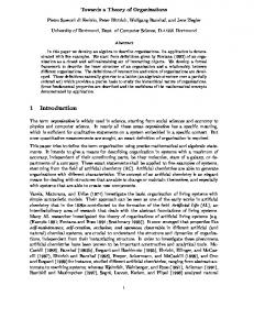
We illustrate the idea of deception through a simple zero-sum game. As explained in introduction, this will allow us to suggest a new motive for reputation building that is not related to the commitment idea. Two players, a Row player and a Column player, play twice, in two consecutive periods, a zero-sum stage game, G. In game G the Row player chooses an action U , D, or B, the Column player chooses an action L or R, and stage game payo¤s are as represented in Figure 1. Players do not discount payo¤s between the two periods, and their overall payo¤ is simply the sum of the payo¤s obtained in the two periods.

U D B

L R 5, -5 3, -3 0, 0 7, -7 11/2, -11/2 0, 0

Figure 1. The stage game G

pay attention only to a limited number of regularities) whereas Bazerman’s discussion of bounded awareness is more about the understanding of the rules of the game. Bazerman’s book also discusses various self-serving biases in decision making and attribute them to the fact that people are "imperfect information processors" (chapter 1). This paper completely agrees with the latter view, and it illustrates how imperfections in the information processing may lead to the possibility of deception. 22 While Khaneman et al. (1982) identify a number of these biases, Thaler (1991) also shows their signi…cance in experimental economics. A number of economists have also developed theories motivated by these biases (see, for example, Mullainathan (2002) or Rabin (2002)).

8


When players are rational, they play the unique Nash equilibrium of the stage game in every period. The Row player plays U with probability 7=9 and D with probability 2=9 and the Column player plays L with probability 4=9 and R with probability 5=9. The overall value of the two-period game is 70=9 for the Row player and 70=9 for the Column player. In equilibrium players play in mixed strategies in order to avoid being predictable. But, note that no player is ever deceived by his opponent: Whatever players do in the …rst period they are expected to play according to the same mixed strategy in the second period, and players do behave according to that expected mixed strategy in period two. As a matter of fact, in a zero-sum game like the one considered here a player can secure his value no matter what the other player does. Thus, with the standard approach there is no point in deceiving the opponent as this could only lower one’s own payo¤. We now consider a setup with boundedly rational players. In our setup, deception may pay (even in the above zero-sum game) because the erroneous inference process of the opponent may lead the latter to think that he can do better than using his minmax strategy (thereby opening the door to the possibility of exploitation). Speci…cally, we consider two types of Row players, the Rational type and the Coarse type assumed to be equally likely. The Rational Row player has a perfect understanding of the strategy of the Column player, as in the standard case. The Coarse Row player knows (or learns) only the average behavioral strategy of the Column player all over the two time periods. That is, the Coarse Row player has only an expectation about the average behavior of the Column player all over the game (i.e., he bundles the two time periods into one analogy class). There is one type for the Column player. The Column player is assumed to be Sophisticated in the sense that he distinguishes between the behaviors of the Rational Row player and the Coarse Row player. But, he is assumed to be Coarse in the sense that for each type of the Row player he knows (or learns) only the average behavior of this type over the two time periods, i.e. the two time periods are bundled into one analogy class. In short, we say that the Column player is a Sophisticated Coarse player. In the next Section we de…ne formally a solution concept called the Analogy-based Perfect Bayesian Equilibrium that describes the equilibrium interaction in such a setup. In a nutshell, equilibrium requires that players play best-responses to their analogy-based expectations (and belief systems), and that analogy-based expectations are correct whereas the updating of the beliefs is assumed to follow Bayes’law as derived from the analogy-based expectations. We will now check that the following strategy pro…le is an Analogy-based Perfect Bayesian Equilibrium: Rational Row Player: Play U in period 1. Play D in period 2 if U was played in period 1, and U otherwise.

9


Coarse Row Player: Play U both in periods 1 and 2. Column Player (Sophisticated Coarse): Play L in period 1. Play R in period 2 if the Row player played U in period 1. Play L in period 2 if the Row player played D or B in period 1. According to this strategy pro…le, (U; L) is played in period 1, and (D; R) and (U; R) are each played with equal probability in period 2 (depending on whether the Row player is Rational or Coarse). Thus, the Column Player plays L and R with an equal frequency on average over the two time periods, and this is the expectation of the Coarse Row player. Given his expectation, the Coarse Row player …nds it optimal to play U whenever he has to move.23 Clearly, the Rational Row player plays a best-response to the Column player’strategy (he gets an overall payo¤ of 5 + 7 = 12 and would only get an overall payo¤ of 0 + 11=2 at best if he were to play D in period 1, a payo¤ of 11=2 + 11=2 = 11 at best if he were to play B in period 1, and he would obviously get a lower payo¤ by playing U or B in period 2). How do we rationalize the behavior of the Sophisticated Coarse Column player ? The Coarse Row player always plays U , and the Rational Row player plays U and D with an equal frequency on average. These (average) behaviors of the two types of Row players de…ne the analogy-based expectations of the Column player. Given these expectations, the Column player updates her belief about the type of the Row player as follows: When action D is being played in period 1, the Column player believes that she faces the Rational player for sure;24 We also assume that this is her belief after action B is being played in period 1.25 When action U is being played in period 1, the Column player believes that she faces the 1=2 Coarse Row player with probability 1=2+1=2 = 23 . This is the posterior belief that derives 1=2 from Bayes’law given the prior and the analogy-based expectations of the Column player. Given the above expectation and belief system, it is a routine exercise to check that the Column player’s behavior is optimal in periods 1 and 2. In period 2 after action D or B has been played, the Column player believes that she faces the Rational Row player with probability 1 and her expectation about this player’s behavior is that he plays U and D with an equal probability. It is then optimal for the Column player to play L (as 1 ( 5 + 0) > 12 ( 3 7)). In period 2 after action U has been played, the Column player 2 believes that she faces the Coarse Row player with probability 32 (and this type is expected to play U always) or the Rational player with probability 31 (and this type is expected to play U and D each with probability 21 ). So overall in period 2 after U has been played in period 1, the This is because 12 (5 + 3) > max[ 12 (0 + 7), 12 (11=2 + 0)] . D is never played by the Coarse Row player. 25 Action B is never played in equilibrium; so action B could come from either type. The chosen belief can be rationalized by assuming that with some small probability the Rational Row player trembles and plays B. 23

24

10


Column player expects the Row player to play U with probability 2=3 1 + 1=3 1=2 = 5=6 and D with probability 1=6. The Column player chooses optimally to play R in this case (since 56 ( 3) + 16 ( 7) > 56 ( 5)). In period 1, the Column player believes it is equally likely that the Row player is Coarse or Rational (this is the prior). Thus, overall in period 1 the Column player expects the Row player to play U with probability 1=2 1 + 1=2 1=2 = 3=4 and D with probability 1=4. The Column player optimally chooses to play L in period 1 (since 34 ( 3) + 14 ( 7) < 34 ( 5)). To summarize, a Rational Row player gets an overall payo¤ of 12, a Coarse Row player gets an overall payo¤ of 8, and the expected payo¤ of the Sophisticated Coarse Column player is 10. Note that the Sophisticated Coarse Row player gets an expected payo¤ smaller than her value ( 10 < 70=9), and both types of the Row player get more than their value. A key feature of the example is deception. By playing U in the …rst period, the Rational Row player makes the Column player (erroneously) believe that he is more likely to be the Coarse type than the Rational type (because U is more ”typical” of the Coarse type than of the Rational type). Because the Column player is su¢ ciently con…dent that she is facing the Coarse Row player and this player plays U always, the Column player …nds it optimal to play R in the second period. The Rational Row player can then safely exploit this erroneous expectation and get a payo¤ of 7 in period 2 by playing D. Observe that deceiving the Column player in period 1 has an immediate cost for the Row player (by playing B instead of U , the Row player could get 11=2 instead of 5), but the immediate cost is more than compensated by the reward he obtains in period 2 after exploiting the erroneous belief of the Column player. If the Column player were fully rational, she would play R in the …rst period and her updated belief after observing U in the …rst period would coincide with the prior (action U in the …rst period is not informative of the Row player’s type). Accordingly, the Column player if fully rational would play L in period 2 (this is the best-response to the expectation that the Row player plays U when Rational and D when Coarse and the belief that the two types are equally likely). Hence, the Rational Row player would only get 3 + 0 under such a scenario and the enterprise of mimicking the Coarse Row player in the …rst period would turn out to be quite suboptimal. More generally, if the Column player were fully rational, she could secure her value 70=9 whatever the strategy of the Row player, and in the present scenario with Coarse and Rational Row players in equal proportion the equilibrium would be such that all players get their value whatever their type.26 26

Observe that if there were only one type for each player characterized by his analogy partition as in Jehiel (2005), then it would be impossible to reproduce the behavioral strategies as described above: For the Column player to play a di¤erent action in periods 1 and 2 she should either be indi¤erent between playing L or R (which cannot be the case here since the Row player does not play U with probability 7=9 on average) or treat separately the behavior of the Row in the two time periods, but then in period 1 she could not …nd it optimal to play L given that the Row player always plays U .

11


Comment : Our zero-sum game example suggests a new perspective on the theory of reputation. When the cognitive abilities of the players are imperfect, reputational concerns may arise, even in games in which there is no value to commitment. Most of the literature on reputation has not considered zero-sum games (because reputation was viewed as requiring commitment value, see Fudenberg and Levine (1989) or Fudenberg and Tirole (1991), ch 9). A notable exception is Crawford (2003)27 who analyzes in the crazy type paradigm a zero-sum game preceded by one round of cheap talk. When behavioral (or crazy) types are su¢ ciently numerous, Crawford (2003) shows that rational types can exploit the presence of behavioral types and get more than their values.28 We wish to emphasize that in Crawford’s model (as well as in the entire literature based on the crazy type approach) those agents who make inferences are fully rational and as such cannot be deceived in equilibrium (they have a perfect understanding of the strategy followed by the opponent). So if a non-behavioral agent (that is, an agent whose behavior is determined endogenously) can get more than his value in Crawford’s model, he can never get less because all such types are perfectly rational (contrast this with our …nding about the Sophisticated Coarse Column player who is nonmechanical - her behavior is endogenous - and yet gets less than her value). We believe that our approach is the …rst one to allow for endogenous fooling in equilibrium. More work is required to understand reputational concerns in our setup when the underlying stage game is repeated over many periods.

3

A general framework

The aim of this Section is to provide a general framework to analyze the interactions of agents with limited cognitive abilities of the type described above. The construction follows those of the Perfect Bayesian Nash Equilibrium (see Fudenberg and Tirole (1991)), and the Analogy-based Expectation Equilibrium (Jehiel (2005)). A reader interested in applications may jump into Section 4.

3.1

The class of games

We consider multi-stage games with complete information. We assume that actions are observable, and we restrict attention to …nite games with two players i = 1; 2 (and possibly Nature). That is, there is a …nite number of stages and, at every stage and for every player (including Nature), the set of pure actions is …nite. This class of …nite multi-stage games is referred to as . 27

Crawford (2003) builds on Hendricks and McAfee (2005). When there are not so many behavioral types, all players whether rational or behavioral get their value in Crawford’s model. 28

12

The standard representation of an extensive form game in class includes the game tree , and the VNM preferences ui of every player i de…ned on lotteries over outcomes in the game. A node in the game tree is denoted by n, and N is the set of all nodes, while Ni is the set of nodes at which player i must move. For every node n 2 Ni , we let Ai (n) denote player i’s action space at node n. A node n will also be identi…ed with the history h of play that leads to node n. The set of players who must move after history h is denoted by I(h), and ha is the history starting with h and followed by a where a 2 Ai (h) is the action proi2I(h)


…le played (by the players who must move) at node h. The set of all histories is denoted by H. Cognitive types: Cognitive types are de…ned as follows. Each player i forms an expectation about the behavior of the other player by pooling together several nodes in which the other player must move. Each such pool of nodes is referred to as a class of analogy. Players are also di¤erentiated according to whether or not they distinguish between the behaviors of the various types of their opponent. Formally, a cognitive type i of player i is characterized by (Ani ; i ) where Ani stands for player i’s analogy partition and i is a dummy variable that speci…es whether or not type i distinguishes between the behaviors of the various types j of player j. We let i = 1 when type i distinguishes between types j ’s behaviors and i = 0 otherwise. Following Jehiel (2005), type i ’s analogy grouping Ani is de…ned as a partition of the set Nj of player j’ s nodes nodes into subsets i called analogy classes.29 When n and n0 are in the same analogy class i , it is required that Aj (n) = Aj (n0 ). That is, in two nodes n and n0 that player i treats by analogy, the action space of player j should be the same, and A( i ) denotes the common action space in i . The set of types i is denoted by i and the pro…le of type space is denoted by = 1 2: Strategic environment: A strategic environment is described by ( ; ui ; p) where p denotes the prior joint distribution on the type space = 1 2 : To simplify notation we will assume that the types of the two players are independently distributed from each other, and we will refer to pi = (p i ) 2 i as the prior probability of player i’s type where p i denotes the prior probability of type i . 29

A partition of a set X is a collection of subsets xk

X such that

S k

13

xk = X and xk \ xk0 = ; for k 6= k 0 .

3.2

Solution Concept


Analogy-based expectations: An analogy-based expectation for player i of type i is denoted by i . It speci…es for every analogy class i of type i of player i a probability measure over the action space A( i ) of player j. Types j of player j are distinguished according to whether i = 1 or 0. If i = 1, i is a function of j and i , and i ( j ; i ) is type i -player i’s expectation about the average behavior of player j with type j in class i . If i = 0, player i merges the behaviors of all types j of player j, and i is a sole function of i : i ( i ) is player i’s expectation about the average behavior of player j in class i (where the average is taken over all possible types). We let i = ( i ) i 2 i denote the analogy-based expectation of player i for the various possible types i 2 i . Strategy: A behavioral strategy (for an arbitrary type i ) of player i is denoted by si . It is a mapping that assigns to each node n 2 Ni at which player i must move a distribution over player i’s action space at that node.30 We let i denote the behavioral strategy of type i , and for every n 2 Ni we let i (n) 2 Ai (n) denote the distribution over Ai (n) according to which player i of type i selects actions in Ai (n) when at node n. We let i (n)[ai ] be the corresponding probability that type i plays ai 2 Ai (n); and we let i = ( i ) i denote the strategy of player i for the various possible types i ; will denote the strategy pro…le of the two players. Belief system: When player i distinguishes the types of player j, i.e. i = 1, he holds a belief about the type of his opponent and this belief may typically change from one node to another. Formally, we let i denote the belief system of player i of type i = (Ani ; i ), where i (h)[ j ] is the probability that player i of type i assigns to the event ”player j is of type j ” conditional on the history h being realized. When player i does not distinguish the types of player j, no belief system is required. To save on notation, we assume that in this case player i ’s belief coincides with the prior pj throughout the game. We call i the belief system of player i for the various possible types be the pro…le of belief systems for the two players i = 1; 2. i , and we let Sequential rationality: From his analogy-based expectation i , player i of type i infers the following representation of player j’s strategy: In all nodes n of the analogy class i player j is perceived to 30

Mixed strategies and behavioral strategies are equivalent since we consider games of perfect recall.

14


behave according to the average behavior in class i as given by i .31 The induced strategy depends on the type j of player j whenever i = 1 (but not when i = 0). At every node where he must play, player i is assumed to play a best-response to this perceived strategy of player j. Formally, we de…ne the i -perceived strategy of player j, j i , as If

i

= 1

If

i

= 0

i j i j

(n) =

i

(n) =

i

( j;

i)

for every n 2

( i ) for every n 2

i

i

and

and j

2

j

2

j

j

Given the strategy si of player i and given history h, we let si jh denote the continuation strategy of player i induced by si from history h onwards. We also let uhi (si jh ; sj jh ) denote the expected payo¤ obtained by player i when history h has been realized, and players i and j behave according to si and sj , respectively. De…nition 1 (Criterion) Player i’s strategy i is a sequential best-response to ( i ; only if for all i such that pi ( i ) > 0, for all strategies si and all nodes n 2 Ni ,32 X j2

j

(n)[ j ]uni ( i

i

jn ;

i j

jn )

X j2

j

i

(n)[ j ]uni (si jn ;

i j

i)

if and

jn )

Consistency: In equilibrium, two notions of consistency are required: the …rst consistency requirement relates the analogy-based expectations to the strategy pro…le; the second one relates the belief systems to the analogy-based expectations. We start with the consistency of the analogy-based expectations. Analogy-based expectations are required in equilibrium to coincide with the real average behaviors in every considered class and for every possible type (if types are di¤erentiated) where the weight given to the various elements of an analogy class must itself be consistent with the real probabilities of visits of these various elements. We will later on suggest a learning interpretation for this consistency requirement. Here is the formal de…nition of consistency where P ( i ; j ; n) denotes the probability that node n is reached when players i and j are of types 33 i and j respectively, and players play according to .

31

This is the simplest representation compatible with type i ’s knowledge. Remember that node n is identi…ed with the history h that leads to it. 33 De…nition 2 places no restrictions on player i’s expectations about those analogy classes that are not reached according to . A stronger notion of consistency would require that the expectations in this case correspond to limits of expectations that would be consistent with small perturbations of . (Such a notion is in the spirit of sequential equilibria - see Kreps and Wilson (1982) - and is discussed in Jehiel (2005) in a simpler context. We have chosen to present the weaker notion of consistency for expositional purposes.) 32

15

De…nition 2 Player i’s analogy based expectation if and only if: For any ( i ;

j)

2

such that ( j; i

whenever there exist For any

i

2

whenever there exist

i

( i) = 0 i,

=

0 j

= 1, and for all

P

( 0i ;n)2

and n 2

such that

i


0 i

i)

i

i

P

i

i

( 0i ;n)2

i

i

0 j ;n)2

P

( 0i ;

and n 2

i

0 j ;n)2

i

2 Ani ,

p 0i P

such that P ( 0i ;

i

( 0i ;

i

p 0i P ( 0i ;

= 0, and for all P

is consistent with the strategy pro…le

i

(n) j ; n) j 0 ( i ; j ; n)

j ; n)

2 Ani ,

p 0i p 0j P ( 0i ; i

> 0:

p 0i p 0j P

such that P ( 0i ;

0 0 (n) j ; n) j 0 0 ( i ; j ; n) 0 j ; n)

> 0.

The consistency of the analogy-based expectations should be thought of as a result of a learning process. Speci…cally, assume that there are populations of players i and j who are repeatedly and randomly matched to play the game. In the population of players i, there is a proportion p i of players of type i . After the end of a session, the behaviors of all the players and their types are revealed. All pieces of information are gathered in a general data set, but players have di¤erent access to this data set depending on their types. A player i with type i = (Ani ; i ) such that i = 0 has access to the average empirical distribution of behavior in every analogy class i 2 Ani where the average is taken over all nodes n 2 i and over the entire population of players j. A player with type i = (Ani ; i ) such that i = 1 has access to the average empirical distribution of behavior in every i 2 Ani for each subpopulation of types j of players j. At each round of the learning process, players choose their strategy as a function of the feedback they received, which in turn generates new data for the next round. Now suppose that the true pattern of behavior adopted by the players is that described by the strategy pro…le . A player i with type i = (Ani ; i ) such that i = 1 will collect data about the average behavior of types j in every class i 2 Ani as soon as a player j with type j reaches some node n 2 i with positive probability (according to ). In the long run, every such statistic should converge (in Cesaro’s sense) and the limit point should be an average of what player j with type j actually does at each of the nodes n where n 2 i , that is, j (n). The weighting of j (n) should also coincide with the frequency with which n is visited (according to ) relative to other elements in i , hence the above expression for ( j ; i ). A similar argument applies when i = 0 for i ( i ). i

16

Comment: In the above learning story we have assumed that there was a common pool of data. An alternative speci…cation would be that types i of players i have access only to those plays where player i was of type i . This would lead to an alternative notion of consistency, but the spirit of the examples discussed in the paper would continue to hold under this alternative speci…cation.


The second consistency requirement relates players’belief systems to their analogy-based expectations. The analogy-based expectation i of player i with type i = (Ani ; i ), i = 1 allows him to distinguish between the behaviors of players j with di¤erent types. As the game proceeds, player i updates his belief about the type of player j using Bayes’ rule (whenever applicable) and assuming that type j behaves according to i ’s perception (see i above). j De…nition 3 Player i’s belief system i is consistent with the analogy based expectation if and only if for any ( i ; j ) 2 such that i = 1 i

i

( j )(;) = p j :

And for all histories h, ha i

(ha)[ j ] =

i

( j )(ha) = P i

(h)[ j ] whenever h 2 = Nj i 0 j2

(h)[ j ]

j

i

i j

(h)[aj ]

(h)[ 0j ]

whenever h 2 Nj , there exists

0 j

0 j

i

(h)[aj ]

s.t.

0 j

i

(h)[aj ] > 0 and player j plays aj at h:

Comment: The consistency of the belief system i with the analogy-based expectation i should be thought of as resulting from an introspective calculus of player i. Based on his representation of the strategy of his opponent for the various possible types he makes inferences (using Bayes’law) as to the likelihood of the various possible types he is facing. This should be contrasted with our learning interpretation of the consistency requirement for the analogy-based expectations (see above De…nition 2).34 Equilibrium: At every node, players play best-responses to their analogy-based expectations (sequential rationality) and both analogy-based expectations and belief systems are consistent. De…nition 4 A strategy pro…le

is an Analogy-based Perfect Bayesian Equilibrium if and

34

A frequentist interpretation of the consistency requirement is also possible, but the eductive interpretation is more in line with the modeling of an inference process.

17

only if there exist analogy-based expectations player i:


1. 2. 3.

i i i

is a sequential best-response to ( i ; is consistent with and is consistent with i .

i

and belief systems

i

such that for every

i ),

An Analogy-based Perfect Bayesian Equilibrium is conceptually very di¤erent from a Perfect Bayesian Equilibrium with incomplete information. The types in our setup are not characterized by their preferences and their information partitions, but by their cognitive abilities to understand (or learn) the strategy of their opponents. This is a totally new notion of types that cannot be interpreted with the standard approach.35 Furthermore, the inference process of the players is not the standard one (even though it is as structured as the standard one, once the analogy partitions are …xed). In the next two sections, we apply the approach to several economic problems. Before moving to these applications, we make two preliminary observations. Proposition 1 In …nite environments, there always exists at least one Analogy-based Perfect Bayesian Equilibrium. Proof: The proof follows standard methods, …rst noting the existence of equilibria in which each player i is constrained to play any action ai 2 Ai (n) at any node n 2 Ni with a probability no less than ", and then by showing that the limit as " tends to 0 of such strategy pro…les is an Analogy-based Perfect Bayesian Equilibrium. Q. E. D. Proposition 2 Consider an Analogy-based Perfect Bayesian Equilibrium of an environment in which one of the types of player i is rational.36 Then this type of player i gets the highest equilibrium expected payo¤ among all types of player i. Proof: The rational type of player i can always mimic the behavior of any other type i of player i, thereby ensuring that he can get at least the expected payo¤ obtained by any other type. Q. E. D. Comment: The result of Proposition 2 should be contrasted with results suggesting that irrational types may perform better in equilibrium. Here it is a comparison of the equilibrium 35

Even when each player i can be of only one cognitive type characterized by his analogy partition, Jehiel (2005) notes that an Analogy-based Expectation Equilibrium cannot be viewed as a standard BayesNash equilibrium of another game with modi…ed information structure. A fortiori when there are several possible cognitive types, an Analogy-based Perfect Bayesian Equilibrium cannot be interpreted as a standard equilibrium of another game with a modi…ed information structure. 36 A rational type is characterized by an analogy partition that is …nest. Whether he can or cannot di¤erentiate the various types of his opponent ( i = 1 or 0) is irrelevant when he has the …nest analogy partition.

18

payo¤s obtained by di¤erent types within the same equilibrium. It is not a comparison of equilibrium payo¤s of the rational types vs the irrational ones when one switches from an environment with only rational types to an environment with only irrational types.


4

The monitoring game

We consider the following stylized monitoring game. At date t = 0, an employee decides whether to Work (exert e¤ort) or Shirk. After observing the employee’s date t = 0 decision, the employer decides at t = 1 whether to Delegate the decision making to the employee (give him discretion) or Control him. At each of the next two dates t = 2; 3, the employee decides whether to Shirk or Work. Payo¤s are speci…ed so that the employee does not like working unless he is controlled, and the cost of control (for the employer) is less than the bene…t that results from the employee working. Speci…cally, if the employee works at t = 0, he gets 0 and the employer gets 1. If the employee shirks at t = 0, he gets 1 and the employer gets 0. Whenever the employer chooses to control (C), shirking at t = 2; 3 is costly to the employee but not to the employer who gets 2 whatever the employee’s choices at t = 2; 3. The employee’s pay-o¤ is strictly decreasing in the number of times he shirks at t = 2; 3: He gets 2 if he works twice; 1 if he works once and shirks once; and 0 if he shirks twice.37 Whenever the employer chooses to delegate (D), her payo¤ is strictly increasing in the number of times the employee works at t = 2; 3. If the employee shirks twice, the employer gets 0, if he shirks once and works once, the employer gets 2 and if he works twice, the employer gets 3. The pay-o¤ of the employee is strictly decreasing in the number of times he works at t = 2; 3: He gets 1 if he never shirks; 2 if he shirks once; and 4 if he shirks twice. The game is represented in …gure 2. The standard analysis of this monitoring game is as follows. The date t = 0 employee’s decision to work (or shirk) is sunk. So he should optimally decide to Shirk. Then the employer should decide to Control so as to make the employee Work (the employee would not work otherwise). The employee gets 3 and the employer gets 2. Consider now the following cognitive environment. There are two types of employees: the Coarse employees and the Rational employees. Employers are assumed to be Sophisticated Coarse. That is, employers make their inferences about the type of their employees based solely on the overall frequency with which the various types of employees shirk. In view of the psychology literature mentioned in introduction, employers are subject to the Fundamental Attribution Error: they base their judgement (about the type of their employees) based on 37

An interpretation of the control technology is that it is such that the employee always ful…lls his task. If he shirks, he is punished and eventually does what he should do.

19


the overall working attitude without paying attention to the situation (date t = 0 or 2; 3) in which the work/shirk decision is made. Formally, Coarse employees put in the same analogy class all the decision nodes in which the employer has to make a decision, and Rational employees use two analogy classes, one for each decision node of the employer. The employee is Coarse with probability 2=3 and Rational with probability 1=3. The Sophisticated Coarse employer uses a unique analogy class that contains all the decision nodes of the employee, and she distinguishes between the behaviors of the two di¤erent types of employees, i.e. 2 = 1. We …rst observe that the behaviors generated by the standard rationality framework are no longer part of an equilibrium in this cognitive environment. If it were, then the belief of the employer should be that the employee works with probability 2=3. But, with such a belief, the employer would choose to Delegate and not to Control.38 As it turns out there is a unique equilibrium in pure strategies in this environment: Proposition 3 The game has a unique Analogy-based Perfect Bayesian Equilibrium in pure strategies. At t = 0, the employee shirks when Coarse and works when Rational. In the last two periods, the employee, whatever his type and his behavior at t = 0, shirks if the employer chooses to delegate (D) and works if the employer chooses to control (C) at t = 1. The employer chooses to delegate (D) if he observes that the employee works in period 1 and to control (C) if he observes that the employee shirks in period 1. In equilibrium, whenever the employee is Rational, he works at date t = 0, the employer chooses to delegate D at date t = 0, and the employee shirks at dates t = 2; 3. Whenever the employee is Coarse, he shirks in the …rst period, the employer chooses C and the employee works in periods 2 and 3. A Rational employee gets 4, a Coarse employee gets 3 and the expected payo¤ of the employer is 5=3. Compared to what happens when all agents are rational, a Coarse employee gets the same payo¤ as in the rational paradigm (!), a Rational employee obtains a higher payo¤ and the employer gets a lower expected payo¤. How do we rationalize these behaviors? In particular, why does the employer choose to delegate to the Rational employee given the cost attached to not controlling? Of course, our premise is that the employer is not aware of the structure of the game (including the objectives of the employee). She has only learned that a Coarse employee works two thirds of the time, and a Rational employee one third of the time (these are the frequencies that result from the proposed strategies). Accordingly, she perceives a Coarse employee to be a (relatively) working employee and a Rational employee to be a (relatively) shirking employee. 38

He would choose D and not C because ( 23 )2

3 + ( 13 )2

20

0 + 2( 13 )( 23 )

2 > 2.


When the employer chooses between D and C, she cares about the type of her employee insofar as it is indicative of whether the employee is perceived to be working or shirking. A key aspect of her decision is governed by her updated belief after she observes the employee’s action at date t = 0. When she observes that the employee works at t = 0, she puts more weight on the probability that the employee is the working type. The employer chooses to delegate, i.e. D, because she is su¢ ciently con…dent that her employee will work next with a high probability. Symmetrically, when the employee shirks at t = 0, the employer puts more weight on the probability that the employee is a shirking type (while he is, with probability 1, a Coarse employee of the working type). She chooses to control. Rationalizing the behavior of the employee at date t = 0 is now an easy exercise. A Coarse employee puts the two decision nodes of the employer in the same analogy class. Accordingly, he decides to shirk in period 1 because he fails to recognize that the employer’s decision to Control depends on the date t = 0 decision to Work.39 A Rational employee perceives that by working in the …rst period, he will deceive the employer who will believe that he is more likely to be of the working type. Even though working induces an immediate loss of 1 at date t = 0, it is worth doing because it leads the employer to delegate next, thereby yielding an extra pro…t of 2 at t = 2; 3 (2 is equal to the di¤erence between what he gets if the employer chooses D and he shirks twice and what he gets if the employer chooses C and he works twice). Our monitoring example captures important features of the deception process. In equilibrium, the Rational employee manages to convey a false belief about his type. The employer is deceived by the Rational employee who behaves in the …rst period in a way that the Coarse employer associates with the Coarse employee (he works). The employer subsequently chooses to delegate the decision power, and she is eventually exploited in the sense that she gets a lower payo¤ than what she would have gotten by controlling the employee. What is striking here is that the Coarse employee (rightly considered to be a relatively working type) does not even work at t = 0, he shirks. The Rational employee in order to be confused with a Coarse employee follows at t = 0 the most frequent behavior of a Coarse employee, even though in this speci…c situation a Coarse employee would not even behave that way. We recognize here standard swindlers’stratagems. The swindler tries initially to build a con…dence relationship with his prey. To do so, in the …rst interactions, he follows an excessively honest behavior (even a standard honest agent would not behave that way). The coarse prey infers from this behavior that the agent he is facing is honest. He drops his guard and the swindler takes advantage of it in the following periods. The swindler’s strategy relies on the coarseness of his prey who wrongly interprets his initial extreme honesty.40 A 39

Ironically, this perception is the right one in the standard rationality paradigm. This phenomenon is well exposed in many movies such as ”The House of Games” (1987) by David Mamet, “The Sting” (1973) by George Roy Hill, The Hustler (1961) by Robert Rossen or “The Color of Money” (1986) by Martin Scorsese (in these two movies, honest is replace by bad pool player ). 40

21


rational prey would rightly interpret this excessively honest behavior of the swindler in the initial periods, “too good to be true” or “too nice to be honest”, and would not believe in the honesty of the swindler. But, a boundedly rational prey as shown in this example can be deceived. Another view on this monitoring example is that because the employer is boundedly rational she does not perceive the interaction with the employee as one with moral hazard. Instead she thinks she is facing an adverse selection problem, and the employer’s concern is about how to adapt the monitoring scheme (control or delegate) to the type of the employee (hard worker or shirking). But, it should be noted here that the mis-speci…cation of the employer’s model derives from the coarseness on the cues used by her. It is not a misspeci…cation assumed exogenously. More generally, the example illustrates that whenever agents base their decisions and inference processes on a limited number of cues, they may be induced to have wrong models and wrong causalities in mind.

5

Deception as a bargaining tactic

Deception is a widespread phenomenon in negotiations. We suggest two simple forms that deception might take in bargaining interactions.

5.1

A concession game

The …rst example is a concession game in which parties alternate in making concessions and they may ask for the intervention of a mediator. Here, deception takes the form that an early concession is meant to (falsely) reassure the other party about one own’s willingness to make further concessions later on. This is illustrated through the following stylized model. Two risk-neutral agents negotiate over the division of a pie of size 400. The negotiation is represented by a series of reciprocal concessions of …xed size. A player, when it is his turn to move, must choose between two options. He can either concede one fourth of the pie to the other player or he can ask for the intervention of an external mediator. If he chooses to concede and after his concession there is something left to be conceded, in the next period, it is the other player’s turn to face the same choice. If a player asks for the intervention of the mediator, what has not been conceded yet is split into two equal shares between the two parties. The party who asked for the mediator’s intervention must pay a commission fee, c, equal to 7% of the share of the pie that the mediator has to split. The game ends when the pie is completely distributed among the two players either through reciprocal concessions, in the fourth period, or after the intervention of the mediator. When a player asks for the intervention of the mediator, we say that he opts out. The corresponding game tree is represented in …gure 2 where payo¤s have been re-

22


normalized by subtracting 150 from player 1 ’s payo¤s and 200 from player 2’s payo¤s. It has a payo¤ structure similar to the centipede game (Rosenthal 1982). Accordingly, in the standard approach, no one wants to be the last to make a concession (he would rather prefer opting out instead). This in turn induces an unravelling e¤ect, and equilibrium entails that there is no concession at all. As a result, the mediator gets a very large share of the pie (he gets 7% of 400, i.e. 28). Consider now the following cognitive environment. With probability 13 , player 1 is Coarse and he understands only the frequency of concessions of player 1, i.e. An1 = ffn2 ; n4 gg where n2 and n4 are the decision nodes of player 2. With probability 32 , player 1 is Rational, i.e. An1 = ffn2 g; fn4 gg. Player 2 is Sophisticated and Coarse; that is, he understands the frequency of concessions of player 1 type by type but not node by node, i.e. An2 = ffn1 ; n3 gg where n1 and n3 are the decision nodes of player 1, and 2 = 1. Proposition 4 The following strategy pro…le41 is an Analogy-based Perfect Bayesian Equilibrium: Player 2 concedes in n2 and opts out in n4 . Player 1 when rational concedes in n1 and opts out in n3 . Player 1 when coarse concedes in both n1 and n3 .

The equilibrium outcome can be summarized as follows: With probability 32 the mediator is called at n3 ; with probability 31 he is called at n4 . The expected fee paid to the mediator is equal to 28 . 3 The crucial part of the equilibrium is about understanding the reasoning of player 2 at node n2 and of the coarse player 1 at n3 . The coarse player 1 believes that player 2 concedes with probability 3=4 on average. Thus, he …nds it optimal to concede whenever he has to move (at nodes n1 and n3 ).42 Player 2 concedes at node n2 based on the following reasoning. Rational Players 1 are perceived to concede with probability 1=2 on average.43 Coarse Player 1s are perceived to concede always. Thus, when player 2 sees player 1 conceding at his …rst decision node, his (1=3)1 updated belief is that player 1 is coarse with probability (1=3)1+(2=3)(1=2) = 12 . Combining with the perceptions of the behaviors of player 1’s various types, player 2 believes at node n2 that player 1 will concede with probability ( 12 )( 12 ) + ( 12 )(1) = 34 at node n3 . Based on this expectation, player 2 chooses to concede at n2 (since ( 43 )43 = 129 > 29). 4 Several observations are in order. For concessions to take place with the above speci…ed payo¤s it is vital that player 1 can be of several types and that player 2 has an incorrect 41

The strategy pro…le in which players opt out whatever their types whenever they have to move is also an equilibrium. Together with the equilibrium shown below these are the only equilibria in pure strategies (see Appendix). 42 At the equilibrium, player 2 always concedes in n2 reached with probability 1 and opts out in n4 reached with probability 13 (because rational player 1 opts out at n3 and the probability that player 1 is rational is 2=3). 43 At node n1 he concedes, at node n3 he opts out and these two nodes are met with the same frequency.

23


belief at node n2 about the type of player 1. If player 1 and 2 were each of one type, it would be impossible to observe concessions in equilibrium however these types are speci…ed.44 For alternative speci…cations of the payo¤s though (keeping the centipede like structure), concessions would be possible even if there were one cognitive type for each player (see Jehiel 2005). Observe also that if player 2 did not distinguish between the types of player 1 (i.e. 45 Thus, if we were to add a 2 = 0) at node n2 he would opt out rather than conceding. small proportion of non-Sophisticated Coarse players 2, these players would opt out at node n2 (whereas the behaviors of all other players would be una¤ected). In such a setup, the non-sophisticated coarse player 2 would perform better than the sophisticated coarse player ), thus illustrating that more 2 (the former would get 29 while the latter would get only 43 3 sophistication may hurt in equilibrium.

5.2

A wage negotiation game

Our second bargaining example is a wage negotiation game between a professor and the dean of a university. The professor can generate outside o¤ers but this is costly, and the dean is not ready to pay a wage rise unless he feels there is a signi…cant probability that the professor would leave otherwise. Payo¤s are speci…ed so that in the standard rationality framework the professor’s threat to leave would not be credible, and thus there would be no wage increase. As we will see, the possibility of deception will ensure that a rational professor may sometimes get his wage increase in such a scenario! Speci…cally, the game tree of the wage negotiation is described as follows. At t = 1, the professor chooses between accepting the status quo (SQ) or developing contacts with another university (D) in view of an alternative faculty position in another department. Establishing these contacts costs him > 0. If he develops contacts, the professor asks for a pay rise (> 0) to the dean. At t = 2, the dean decides either to refuse (R) or to accept (A) the pay rise. If the dean accepts, the professor stays in the department and the negotiation process is over. The professor ends up with a higher wage, and he stays in his original position. If the dean refuses, at t = 3, the professor chooses again between accepting the status quo (SQ) staying in his department with his initial salary - or developing further contacts (D) with the other university at cost , getting from it an o¤er. If the professor chooses the second option, 44

It is easy to see that no equilibrium in pure strategy with concessions can be sustained whatever the analogy partitions. Whatever his belief player 2 opts out at n4 . Thus, in a pure strategy equilibrium, the most optimistic belief that player 1 may have (it corresponds to the coarsest analogy grouping) is that player 2 concedes with probability 1=2 on average. With such a belief, player 1 chooses to opt out at n3 . But, then player 2’s belief about 1 is that he concedes at best with probability 1=2. This in turn induces player 2 to opt out at n2 (because 29 > 43=2). Hence, player 1 ’s belief is that player 2 opts out always, and he must opt out at n1 . It is left to the reader to check that there is no equilibrium in mixed strategy either. 45 By de…nition of his type he would not make any updating about the type of his opponent. He would believe that player 1 concedes on average with probability 2=3 and 29 > 86 3 .

24


he goes back to the dean, exhibits his alternative o¤er and asks for a pay rise 0 (> 0).46 At t = 4, the dean decides whether he accepts (A) the pay rise 0 or refuses it (R). The professor stays in the department if the dean accepts the pay rise or leaves the department and goes to the other university if the dean refuses the pay rise.47 If the professor accepts the o¤er of the other university, the original department incurs a cost X and the professor gets U 2 .48 We normalize payo¤s so that in the original situation both the dean and the professor have a pay-o¤ 0. We further assume that X < 0 and U < , and to …x ideas, we let = 3, 0 = 4, = 1, X = 72 and U = 12 . In a perfect rationality world, X < 0 implies that at t = 4, the dean prefers to let the professor go rather than accept the pay rise. Given that there is no pay rise at t = 4, U < implies that at t = 3 the professor does not …nd it useful to generate an outside o¤er of U for an extra cost . Anticipating that no further search e¤ort will be made by the professor, the dean at t = 2, …nds it optimal not to accept the pay raise. Finally, at t = 1, the professor does not develop contacts because he anticipates no pay rise will be accepted. The game is represented in Figure 3 where the …rst and second decision nodes of the professor (resp. dean) are labelled n1 and n3 (resp. n2 and n4 ). In the standard rationality paradigm, even though the professor has the possibility to go for another job, the outside option is perceived as non-credible, and there is no pay rise. This is a stylized and simpli…ed version of the so called outside option principle (see Binmore et al. 1989). Consider now the following cognitive environment. With probability 1=2, the dean is Sophisticated Coarse, he puts in the same analogy class both decision nodes of the professor, i.e. An = ffn1 ; n3 gg, he distinguishes between the various types of the professor, i.e. = 1. With probability 1=2, the dean is Rational, An = ffn1 g; fn2 gg and = 1. With probability 1=2, the professor is Coarse, An = ffn2 ; n4 gg, he puts in the same analogy class both decision nodes of the dean and = 0, he does not distinguish between the various types of the dean. With probability 1=2, the professor is Rational, An = ffn2 g; fn4 gg and = 1. The following proposition illustrates the possibility of search activity and pay rise in equilibrium: Proposition 5 The following strategy pro…le49 is an equilibrium: A Coarse professor establishes contacts with an alternative University whenever he has the opportunity to and a 46

We have in mind that 0 > so that the new pay rise compensates at least partially for the extra search cost. 47 In the latter event, the professor could stay in his original position, but we assume then that the induced atmosphere is quite bad for the professor (colleagues are quite upset). 48 U is equal to the value of the alternative o¤er minus the costs the professor incurs leaving his university. 49 The Subgame Perfect Nash equilibrium strategy pro…le (described earlier) is also an equilibrium. (See the Appendix).

25


Rational professor establishes contacts in n1 and accepts the status quo in n3 . A Sophisticated Coarse dean accepts the pay rise in n2 and refuses to give a pay rise in n4 . A Rational dean always refuses to give a pay rise.

In equilibrium, the professor always makes an e¤ort to get an alternative o¤er at t = 1. With probability 21 , the dean accepts the pay rise; with probability 14 , the professor leaves his department (thus taking the outside option) and, with probability 14 , he stays in his department with his initial salary. We observe that the outside option of the professor which, in the standard rationality paradigm, would be considered as non-credible (and would thus have no e¤ect), does a¤ect the equilibrium play here. The logic of the equilibrium is as follows. First, it is readily veri…ed that the behaviors of the rational professor and the rational dean are optimal. So let us focus on the Coarse professor and the Sophisticated Coarse dean. A Coarse professor perceives that the dean accepts the pay rise with a probability equal 1=2 2 ) on average. For such a high probability of acceptance, it is worthwhile to 5 (= 1+1=4 developing further contacts at t = 3 since 25 ( 0 2 ) + 53 (U 2 ) > . It is also readily veri…ed that a Coarse professor …nds it optimal to develop outside contacts at t = 1. The Sophisticated Coarse dean perceives that a Coarse professor always chooses D and a Rational professor chooses D with probability 32 on average50 . At t = 2, he observes that the professor chose D in n1 . Given this behavior, the Sophisticated Coarse dean’s updated (1=2) belief at n2 is that the Professor is Coarse with probability (1=2)+(1=2)(2=3) = 35 . Combining the perceived behaviors and beliefs, the Sophisticated Coarse dean expects the professor to make further search e¤orts in n3 with probability ( 35 )1 + ( 25 ) 23 = 13 . According to this 15 51 expectation, the dean prefers to accept the pay rise in n2 . It should be noted that the dean accepts the pay rise here because he puts a su¢ ciently high probability on the professor being coarse due to this erroneous belief updating. If the dean were to keep the prior belief that the professor is Coarse with probability 12 (which would be the standard belief at node n2 if the dean were fully rational), he would choose not to accept the pay rise at n2 .52 For rational agents, the presence of boundedly rational agents has two main consequences. First, at the start of the interaction, Rational professors mimic Coarse professors and exert e¤orts towards the outside university. That way, they deceive Coarse deans, and make them believe that they are facing a Coarse professor with a high probability. Coarse deans accept 50

In the …rst node, reached with probability 1, a Rational professor chooses D and in n3 , reached with probability 12 , a Rational professor chooses SQ. Therefore, a Sophisticated Coarse dean perceives that a 1+0 Rational Professor chooses D with a probability 1+1=2 = 23 in the analogy class gathering n1 and n3 . 7 2 51 This is because 3 > 13 15 ( 2 ) + 15 (0). 52 He would have perceived that his payo¤ obtained by not accepting the pay rise is 1235 (= ( 12 1 + 12 2 7 ( 12 1 + 12 23 ))(0)) and he would not have accepted the pay rise (since 1235 > 3). 3 )( 2 ) + (1

26


the pay rise at t = 2 because they are su¢ ciently afraid that the professor would otherwise leave. Second, Rational deans fail to be identi…ed as Rational deans by Coarse professors at t = 3. Coarse professors do not perceive that there exist two types of deans. Thus, even though a Rational dean behaves di¤erently from a Coarse dean at t = 2, a Coarse professor keeps on believing, at t = 3, that the dean will concede with probability 52 at t = 4. In this case, Rational deans would prefer being identi…ed as what they are : Rational deans who never accept pay rises. Coarse professors would then choose the status quo at t = 2 and the rational dean would get 0 rather than 47 (the expected payo¤ in the equilibrium of Proposition 5). This illustrates that it may be costly for a rational agent not to be distinguished from other types due the cognitive limitations of other players.

27

6


6.1

Appendix Proof of Proposition 3

First, a Coarse employee puts the two nodes in which the employer has to make a decision into the same analogy class. Therefore, he always shirks at t = 0. Second, if the employer chooses C, there is a unique best-response for the employee whatever his type and belief are: To work at t = 2; 3. Conversely, if the employer chooses D, there is a unique best-response for the employee whatever his type and belief are: To shirk at t = 2; 3. Therefore, to …nd an equilibrium, we only need to focus on the decision of a Rational employee at t = 0 and the decision of the employer. Choosing D after having observed that the employee shirking at t = 0 cannot be part of an equilibrium strategy since the employee’s best response would be always to shirk. Suppose now that the employer chooses C both if the employee works and if the employee shirks at t = 0. The employee, whatever his type is, has a unique best response: To shirk at t = 0 and to work at t = 2; 3. The employer perceives that an employee, whatever his type is, works with a probability 2/3. C is not a best response to such a belief and choosing C in both cases cannot be part of an equilibrium either. The only remaining possibility for the employer is to choose C (resp: D) when he observes that the employee shirks (resp: works) at t = 0. A Rational employee has a unique best response to such a behavior, to work at t = 0. Now, we need to establish that it exists a belief consistent with these behaviors such that the employer behavior is a best response to this belief. If players follow the described behaviors, a Coarse employee shirks once and works twice and a Rational employee shirks twice and works once. The employer perceives that a Coarse (resp: Rational) employee chooses to work with a probability 2/3 (resp: 1/3). After having observed an employee working at t = 0, her revised belief is that he is Coarse with probability: (2=3)(2=3) = 45 and, if she observes that the employee shirks at t = 0, she believes (2=3)(2=3)+(1=3)(1=3) (1=3)(2=3) that he is Coarse with probability (1=3)(2=3)+(2=3)(1=3) = 12 . Crossing beliefs and analogy-based expectations, we obtain the following. After having observed that the employee shirked (resp: worked) at t = 0, the employer prefers choosing C (resp: D). Q.E.D.

6.2

Proof of Proposition 4

We prove that no other strategies than the one mentioned in Proposition 4 and the strategy pro…le in which players opt out whenever they have the opportunity to can be part of an 28


equilibrium in pure strategies. First, note that it is a strictly dominant strategy for player 2 to opt out in n4 , therefore, at the equilibrium, player 2 always opts out in n4 . By backward induction, we can infer that, at the equilibrium, if player 1 is Rational, he always opts out in n3 . Suppose that player 2 opts out in n2 . If player 1 is Rational, he plays the unique best response, opt out in n1 . Besides, since player 2 opts out in n2 , he always opts out when he is in the analogy class fn2 ; n4 g. Then either player 1 always opts out in n1 or player 1, if he is Sophisticated Coarse, perceives that player 2 always opts out when he is in fn2 ; n4 g. Opting out in n1 and n3 is his unique best-response to such a belief.53 If player 2 opts out in n2 , player 1’best response, whatever his type is, is to opt out in n1 and in n3 . Now, suppose that player 2 concedes in n2 . A Rational player 1 has a unique best response, concede in n1 . Suppose that a Sophisticated Coarse player 1 opts out in n1 or concede in n1 and opts out in n3 . Player 2 concedes in n2 and never has the opportunity to play in n4 . Therefore, whenever nodes n2 or n4 are reached, player 2 concedes. A Sophisticated Coarse player 1 expects player 2 to concede with probability 1 in fn2 ; n4 g . is strategy is not a best-response to his expectation. There only remains two pairs of strategies that can be part of an equilibrium: - Players opt out whenever they have the opportunity to. - Player 1 concedes in n1 whatever his type is. In n3 , if he is Rational, he opts out and if he is Sophisticated Coarse, he concedes. Player 2 concedes in n2 and opts out in n4 . The …rst strategy pro…le is consistent with ( 1 ; 2 ) such that players, whatever their types are, expect that their opponent always opt out. The second strategy pro…le is consistent with ( 1 ; 2 ) such that : (i) Player 2 expects a Rational player 1 to concede with a probability 21 in the analogy class fn1 ; n3 g and a Sophisticated Coarse player 1 to concede with probability 1 in this same analogy class. (ii) A Rational player 1 expects player 2 to concede in n2 and to opt out in n4 . (iii) A Coarse player 1 expects player 2 to concede with a probability 3=4 in fn2 ; n4 g. Q.E.D.

6.3

Proof of Proposition 5

We …rst exhibit two equilibria in pure strategies and leave to the reader to check that there exists no other equilibrium. The …rst equilibrium. Suppose that the dean always refuses to give a pay rise to the professor. Then whatever his type is, it is a best response for the professor to always accept 53

We should also notice that there exists no belief about the average behavior of player 2 in fn2 ; n4 g such that opting out in n1 and conceding in n3 would be a best response to this belief for a Sophisticated Coarse player 1.

29


the status quo since 32 < 1 < 0: Whether the professor gathers in the same analogy class n2 and n4 does not matter since the dean behaves the same way in these two nodes if they are reached. Now, if the professor never develops contacts with another department, it is a best response for the dean never to concede a pay rise since 3 < 0 and 4 < 72 . Again, whether the dean gathers in the same analogy class n1 and n3 does not matter since the professor behaves the same way in these two nodes when they are reached. The second equilibrium. Suppose that a Coarse professor chooses D in n1 and n3 , a Rational professor chooses D in n1 and SQ in n3 , a Sophisticated Coarse dean chooses C in n2 and R in n4 and a Rational professor chooses R in n2 and n4 . First, let us remark that the strategies of the Rational professor and dean are best response to the strategy of the other agents. Now, a Coarse professor perceives that the dean concedes with a probability 1=3 in the analogy class fn2 ; n4 g and a best response to this belief is to choose D in n3 and n1 since 1 < 1 1 + 13 4 + 23 12 and 0 < 1 + 13 3 + 23 [ 1 + 13 4 + 23 12 ]. Besides, a Sophisticated Coarse dean chooses R in n4 since it is a dominant strategy. Now, a Sophisticated Coarse dean expects a Coarse professor always to choose D in fn1 ; n3 g and a Rational professor to choose D with a probability 32 in fn1 ; n3 g. When n2 is reached, a Sophisticated Coarse dean 1 1=2 believes that the professor is Coarse with a probability 1 1=2+2=3 = 35 . He expects the 1=2 7 professor to choose D in n3 with a probability 35 1 + 25 23 = 13 and, since 13 < 3, 15 15 2 the unique best response to his belief and expectation i to concede in n2 . Q.E.D.

30

References [1] Bazerman, M. (2005): Judgment in Managerial Decision Making , 6th edition, Wiley. [2] Binmore, K.,Shaked, A. and Sutton, J. (1989): ’An Oustide Option Experiment’, Quaterly Journal of Economics, 104, 753-770. [3] Crawford, V. P. (2003): ’Lying for Strategic Advantage: Rational and Boundedly Rational Misrepresentation of Intentions’, American Economic Review, 93, 133-149. [4] Darwin, C. (2002): The Expression of The Emotions in Man and Animals, 3rd Edition, Oxford University Press.


[5] Ekman, P. (2003): ’Darwin, Deception and Facial Expression’, in Emotion Inside Out, ed Ekman, P., (1000: 205-221) Annals of the New York Academy of Sciences. [6] Eyster E. and M. Rabin (2005): ’Cursed Equilibrium,’Econometrica 73, 1623-1672. [7] Fudenberg D. and Levine, D. K. (1989): ’Reputation and Equilibrium Selection in Games with a Patient Player’, Econometrica, 57, 759-778. [8] Fudenberg D. and Tirole, J. (1991): Game theory, MIT Press. [9] Gabaix, X. and D. Laibson (2005): ’Consumer myopia, Shrouded Attributes and Information Suppression in Competitive Markets,’mimeo. [10] Gigerenzer, G. and Selten, R. (2002): Bounded Rationality: The Adaptive Toolbox, MIT Press. [11] Gigerenzer, G., Swijtink, Z., Porter, T., Daston, L., Beatty, J. and Krüger, L. (1989): The Empire of Chance. How Probability Changed Science and Everyday Life, Cambridge University Press. [12] Gneezy, U. (2004): ’Deception: The role of consequences,’mimeo. [13] Grimm, J. and Grimm, W. (2001): The Complete Fairy Tales of the Brothers Grimm, Bantam. [14] Hendricks, K. McAfee,R. P. (2005): ’Feints’, Forthcoming Journal of Economics and Management Strategy. [15] Jehiel, P. (2005): ’Analogy-based Expectation Equilibrium’, Journal of Economic Theory 123, 81-104. [16] Jehiel, P. and F. Koessler (2005): ’Revisiting Games of Incomplete Information with Analogy-based Expectations’, mimeo. 31

[17] Jones, E. E. and Davis K. E. (1965): ’From Acts to Dispositions: The Attribution Process in Person Perception’ in Berkowitz L. (ed), Advances in Experimental Social Psychology (Vol 2, 219-266), New York: Academic. [18] Kahnemann, D., Slovic, P. and Tversky, A., eds (1982): Judgement Under Uncertainty, Heuristic and Biases, Cambridge University Press. [19] Kreps, D. , P. Milgrom, J. Roberts and R. Wilson (1982): ’Rational cooperation in the …nitely repeated prisoners’dilemma’, Journal of Economic Theory, 27: 245-252. [20] Kreps, D. and Wilson, R. (1982): ’Sequential Equilibria’, Econometrica, 50: 863-894.


[21] Kreps, D. and Wilson,R. (1982): ’Reputation and Imperfect Information’, Journal of Economic Theory, 27, 253-279. [22] Laibson, D. (2001): ’A cue-theory of Consumption’,Quaterly Journal of Economics, 116, 81-120. [23] Lewis, M. (1990): Liar’s Poker, Penguin Books. [24] Mullainathan, S. (2002): ’A Memory-Based Model of Bounded Rationality’, Quaterly Journal of Economics, 117: 735-774. [25] O’Sullivan, M. (2003): ’The Fundamental Attribution Error in Dectecting Deception: The Boy-Who-Cried-Wolf E¤ect’, Personality and Social Psychology Bulletin, 29, 13161327. [26] Piccione, M. and A. Rubinstein (2003): ’Modelling the Economic Interaction of Consumers with Diverse Abilities to Recognize Equilibrium Patterns,’Journal of European Economic Association 1, 212-223. [27] Rabin, M. (2002): ’Inference by Believers in the Law of Small Numbers’, Quaterly Journal of Economics, 117: 775-816. [28] Rosenthal, R. (1982): ’Games of Perfect Information, Predatory Pricing and the Chain Store Paradox’, Journal of Economic Theory, 25, 92-100. [29] Ross, L. (1977): ’The Intuitive Psychologists and his Shortcomings’in Berkowitz L. (ed), Advances in Experimental Social Psychology (Vol 10, 173-220), New York: Academic. [30] Ross, L., Amabile, T. M. and Steinmetz, J. L.(1977):’Social Roles. Social Control and Biases in Social-Perception Processes’, Journal of Personality and Social Psychology, 35, 485-494. [31] Selten, R. (1978): ’The Chain-Store Paradox’, Theory and Decision, 9, 127-159. 32

[32] Schelling, T. (1960): The Strategy of Con‡ict. Harvard University Press. [33] Simon, H.A. (1956): ’Rational Choice and the Structure of Environment’, Psychological Review, 63: 129-138. [34] Spiegler, R. (2005): ’Competition over Agents with Boundedly Rational Expectations,’ mimeo. [35] Thaler, R.H., (1991): Quasi Rational Economics, Russell Sage. [36] Von Neuman J. and Morgenstern, O. (1944): Theory of Games and Economic Behavior, Princeton University Press.


[37] Vrij, A. (2001): Detecting Lies and Decit. Wiley, New York.

33

1

HH HH H

W


2 D

S H HH HH H2 @ @ D @C @

@

@ @C @

@ @ @1 @1 1 A A A A A A A W W W W AA S AS AS AS A A A A A1 A1 A1 A1 1 1 1 1 A A A A A A A A W AS W AS W AS W AS W AS W AS W AS W AS A A A A A A A A (1,4) (2,3) (2,3) (4,1) (2,3) (1,3) (1,3) (0,3) (2,3) (3,2) (3,2) (5,0) (3,2) (2,2) (2,2) (1,2)

1

Fig.2. The monitoring game

34


n1

C

n2

C

n3

C

n4

O

O

O

O

(22,0)

(0,29)

(36,0)

(0,43)

Fig.3. The Concession Game.

35

C

(50,0)


n1

SQ

(0,0)

D

n2

R

n3

D

n4

A

SQ

A

(2,-3)

(-1,0)

(2,-4)

Fig.4. The Wage Negotiation Game

36

R

(-3/2,-7/2)