pa er presented at the 76th annual meeting of the Association of American ..... patterns on a map, such as the major urban centers in a system of cities, in terms.
Daniel A. GrijJith*
Towards a Theory of Spatial Statistics
Seminal work completed in statistics by Student (1914), Moran (1948), Whit-
tle (1956), Geary (1954), and others, has set the stage for the development of statistical theory that is appropriate for handling geographical problems. These contributions have been followed up with writings by CliE and Ord (1973), Besag (1975), Hepple (1976), and Haining (1978) to mention a few, which focus on the concept of spatial autocorrelation. Unfortunately, this body of literature merely scratches the surface of spatial statistical theory. The general purpose of this article is to illuminate directions for additional work in this area. More specifically, prominent estimation problems concerning the presence of a nonvanishing Jacobian and the effects of geographical boundaries, and interpretation problems pertaining to data transformations will be investigated in order to emphasize existing shortcomings, and then a course for further development will be outlined. THE JACOBIAN DETERMINANT AND SPATIAL AUTOCORRELATION
A popular linear spatial operator associated with spatial autocorrelation is of the form (I - p W). Given n areal units, the elements of matrix W may be defined in such a way that wli 2 0, 2: 1 wv = 1, i = 1,2, . . ., n, and wv = 0 if areal units i and j are not juxtaposed. In other words, this component of the operator casts each areal unit value as a linear function of the average of the contiguous unit values. If p defines the nature and degree of spatial autocorrelation present, then - 1 < p < 1. Now the mathematical mapping from a domain of unautocorrelated values into some geometric space having autocorrelated values requires specification of the differential for this mapping, known as the Jacobian determinant. This determinant serves a dual purpose. First, its sign indicates the orientation of the autocorrelated coordinate system with respect to the unautocorrelated system. A positive Jacobian value means the two systems have equivalent orientations, whereas a negative value means they have opposite orientations. Second, the Jacobian specifies that relationship prevailing between the metrics of these two spaces. Thus for a two-dimensional situation it becomes
*This article is based on the author’s doctoral dissertation and was a Nystrom Competition Finalist pa er presented at the 76th annual meeting of the Association of American Geographers in Louisvile, 1980.
Daniel A . Grtfith is assistant professor of geography, State University of New York at Buffalo.
0016-7363/80/ 1080-0325$00.50/0 0 1980 Ohio State University Press GEOGRAPHICAL ANALYSIS, vol. 12, no. 4 (October 1980) Submitted 8/79. Revised version accepted 4/80.
326 I Geographical Analysis where (u,u) and (x,y ) are coordinates in the unautocorrelated and autocorrelated spaces, respectively, and A denotes area. Hence the Jacobian defines rates of change in the autocorrelated coordinate system in terms of rates of change in its unautocorrelated counterpart. Further, the Jacobian, say J , appears in the mapping from (u,u) to ( x , y ) through the evaluation of some function f(u,v) over a region R in the unautocorrelated space by means of the proper integral over a corresponding region R' in the autocorrelated space such that
In the case of spatial autocorrelation this Jacobian is J = [det (I - p W)] , Clearly as p + 1, J + 03 . But given that I p I < 1then as the number of areal units increases without bound the modified Jacobian term reduces to unity:
lim [det (I - p
= 1,
n+a Moreover, results from spatial statistical analyses often are asymptotically equivalent to those from classical statistical analyses (Hepple 1976), since IJI-2'n = 1means this Jacobian disappears from the right-hand side of equation (1).A salient question at this point, though, has to do with how quickly this Jacobian approaches unity as n + 03. The importance of this question lies in the magnitude of complexity introduced into spatial statistical estimation procedures by the presence of this Jacobian. Because W is a stochastic matrix, then if it is indecomposable (see Alao 1970) the largest eigenvalue is A,, = 1. The Perron-Frobenius theorem of linear algebra insures that A,, is unique, and that even in absolute value terms no other eigenvalue is greater than Am,. Meanwhile, the Jacobian may be rewritten as
=
[(l - p)
iz i=2
(1 - p hi)]
-an,
where hi is the ith eigenvalue of matrix W, and hl = A,, trace of matrix W is zero,
z xi i=n
= 0,
or
i= 1
1+
z xi
Now,
= 1. Because the
i=n
= 0.
i=2
Optimizing ln(2) subject to equation (4) yields
hz=A3=hq=
(3)
. . . An.
(4)
Daniel A . Griffith I 327 i=n
i=n
X = I + ( ~ - ~ ) A = Oor,
1 + C hi=l+ i=2
A =
i=2
-V( n - 1 ) .
(5)
Substituting the critical number -(n -
+p
{(l- P)
(n+)]
into equation (3) results in -2'n
n-11
This value is the minimum value that the Jacobian can assume, since
[1n(z)l2
=
2
2
-
a2 xi
,
and
(1 - p Xi)' 2 n
2
-
l [1 + P (-)I n-1
> O . 2
Constraint equation (4)coupled with this last result imply that if any hi, i # 1, increases in value, then there exists some Xj, j # 1, i, that decrease(s) in value and hence the value of the objective function In(2) must increase. The limit to this process is when X i = 1, i = 1, 2, . . ., k , and X i = -1, i = k 1, k + 2, . . ., 2k, where 2k + y = n, y = 0, 1. If n is even, then y = 0; otherwise y = 1, and = 0. Therefore, the maximum value the Jacobian can assume occurs when matrix W is decomposable, where this value equals
+
One should note that this is a limiting case, since for all n > 2 only one characteristic root will attain a positive value of unity when matrix W is indecomposable. If y = 0, then this expression reduces to
[(l - p) (1
+ p)]-l
= (1 - p2)-'
+
,
If y = 1, then since 2k/(2k 1) < 1, (1 - p2)-2w(2k+1) 5 (1 - p2)-l . Consequently, the maximum value for the Jacobian is (1 - p2)-l . This specific situation is associated with a geographical configuration in which areal units appear only in pairs and hence matrix W is decomposable and is block diagonal such that each block is (PO'). Clearly it is an unlikely configuration, even if a nearest neighbor network were to be envisaged. One contention frequently found in the literature maintains that although presence of this aforementioned Jacobian complicates matters considerably, and usually means resorting to nonlinear estimation methods, the accuracy of results obtained is well worth any extra tedium (Haining 1978). When a geographical arrangement of areal units produces a Jacobian that assumes its minimum value, however, this contention may well be misleading, since for an appropriate value of n, J-'"' = 1 and hence disappears. Consider the results displayed in Table 1. If biases introduced by treating a Jacobian whose value is 1.1 as being 1.0 are tolerable, then any geographical landscape partitioned into at least thirty areal units could be analyzed in a traditional fashion. Similarly, if biases introduced by treating
328 / Geographical Analysis a Jacobian whose value is 1.05 rather than 1.0 are tolerable, then any landscape consisting of at least fifty-eight areal units could be analyzed in a traditional manner. Clearly, the minimum number of areal units necessary is directly related to the degree of prevailing spatial autocorrelation, since the Jacobian approaches CQ as p + 1. Interestingly enough, biases associated with exclusion of the Jacobian appear to be more profound when the autocorrelation is positive than when it is negative. TABLE 1 Critical Values of n for Selected Jacobians i=n
i=l P
maximum Jambian vdue
-0.9
5.263 . _
-0.5
1.333
-0.1
1.101
0.1
1.101
0.5
1.333
0.9
5.263
lmln 1.100 _ _ 1.046 1.010 1.073 1.041 1.010 1.005 1.005 i.005 1.010 1.010 1.005 1.093 1.047 1.010 1.099 1.050 1.010
l-lmin
n
0.10
7 13 54 4 6 21 3 3 3 2 2 3 5 9 40 30 58 283
0.05 0.01 0.10 0.05 0.01 0.10 0.05
o.oi
0.10 0.05 0.01 0.10 0.05 0.01 0.10 0.05 0.01
critical value
min
1.167 1.083 1.019 1.333 1.200 1.050 1.500 1.500 is00 2.000 2.000 1.500 1.250 1.125 1.026 1.034 1.018 1.004
2.448 i.898 1.364 3.473 2.277 1.649 2.000 2.000 2.000 2.000 2.000 2.000 2.442 2.181 1.435 1.518 1.370 1.134
max
6 12 54 4 6 20 2 2
2
2 2 2 4 8 40 30 58 282
x'ow,.
"-1
12.592 2i.026 70.978 7.815 9.488 31.410 5.991 5.991 5.99i 3.841 3.841 5.991 7.815 15.507 54.560 42.557 76.766 318.538
Note:] is the Jacobian value in question: n is the number of areal units
The next question meriting attention is whether or not some set of eigenvalues is sufficiently similar to the set accompanying a Jacobian of minimum value. Presumably the best way to ascertain an answer to this question is through the chi-square relationship x2 = (n - l)s2/a2. Let Xi, i = 1, 2, . . ., n, be the set of eigenvalues under study. From equations (4) and (5) the eigenvalues yi associated with a Jacobian of minimum value were found to be 1, and n -- 1 characteristic roots of -(n - l)-'. Because yi = Z;Zi' Xi = 0, 7 = A = 0, and u2 = 417 y:/n while s2 = 41fiAn/: = {12+ ZiZ;[-(n-1)-1]2}/n = l/(n-1). Thus,
Using the significance test format for i=n
x X : < L L X2> i= 1 (n-1)2
x2, for decision-making purposes,
yields
Daniel A . Griffith I 329 where x2 has n - 1 degrees of freedom. Returning to Table 1 once again, critical values for each of the preceding minimum-value Jacobians are presented. Equation (8) permits one to infer that for a landscape partitioned into, say, thirty areal units, if ZZi' A: < 1.518 then biases introduced by overlooking the Jacobian term will be minuscule. Furthermore, extending equation (6) so that k multiple values of unity appear yields A = -k/(n - k ) # 1. Using this result permits equation (7) to be rewritten as i=n
( n - 1) ( n - k) x2
2 A? i= 1
=
=[
n(n - 1)
s
l 2
A:
i= 1 i= 1 i = n
k =
n
or
>
nk
x2 + ( n - 1)
1 ,k
z A?
1
i=l
qn 2 !n. !
(9)
Equation (9) renders a value for k that becomes useful when Z i I 7 A? exceeds the critical value given in Table 1. As k + 1 the rate of convergence for the Jacobian upon unity is increasingly rapid. In contradistinction, as k +. [ ( n - l)/2] the rate of convergence slows down. Thus, k furnishes an index for assessing the importance of the Jacobian. Nevertheless, unless an extremely small number of areal units is being analyzed, or unless a highly fragmented geographic configuration exists, rewards associated with utilizing the Jacobian may not be justified in terms of the affiliated increase in numerical complexities. For illustrative purposes equation (8) was used to determine whether or not an ordinary least squares estimate of p was acceptable for each of thirty-two agricultural variables measured in Puerto Rico (Griffith 1979). In this case study x2 .05,72 = 92.801, and the critical value for 2Z:3A: is 1.307. The actual sum of squared eigenvalues equaled 15.556. Meanwhile, following equation (9), k = 10 l/(n + 1) .
(4n1’2)l(4n”z
In other words, if 10 percent of the units are to be initially used and then discarded, n = 9 for time series while n = 130 for spatial series. Similarly, if 1 percent of the units are to be initially used and then discarded, n = 99 for time series while n = 1,569 for spatial series. In light of these findings, a second property worthy of exploration refers to the degree of linearity latent in a geographical configuration. Once again, since the eigenvalues of matrix W need to be calculated anyway, this second property will be explored in terms of these n characteristic roots. The indices proposed here are not necessarily better than those that currently exist in the literature. They are just more convenient. First the eigenvalues of matrix W for a linear arrangement of areal units need to be ascertained. This matrix defines the recurrence relation for Chebyshev polynominals of the first kind (Ord 1975). Imposing boundary conditions associated with areal units 1 and n yields as the eigenvalues for matrix W
where the argument of cos is in radians. Equation (10) is the eigenvalue generating function for a linear arrangement of areal units, from which the following two useful theorems may be derived:
2 yi +/[(n+l)/21 i=n
THEOREM 1. V n 2 2,
i=l
i=n
2
THEOREM 2. V n 2 2,
y:
= 1
k=n-1
+
k=l
i= 1
=
1+[- n - 1
n n )sin (n) cos (__ 2 sin (-
2 = 1 +
~
n-1 2
n-1
+
- -n + l -
2
7 n-1
3
Daniel A . Grif-th I 333 These two theorems are proven by direct substitutions into finite series sums provided by Abramowitz and Stegun (1965). These two theorems will now be used to construct indices that will permit the degree of linearity latent in a geographical configuration to be ascertained. Using the significance test format for a mean, for decision-making purposes, yields in the limit
z
he moment generating function of any xi is
-
i=l,2, ..., n . THEOREM5 . Suppose y = (I - py W)-l V and bk[ E (I - py W)-'. Then
Daniel A . Griffith I 335
E(UV)/u,
(T,
*
These three theorems are the source of several interesting implications about the empirical frequency distribution suggested by the xi's. First, theorem 3 indicates that the n marginal distributions associated with the weighted sums XjZ? au uj are different since X&i' aij # XjZ? akj, i # k. This property implies that an empirical frequency distribution based upon the xi's may well deviate from a normal distribution, even though the uls are identically normally distributed. Such a deviation arises because different weights are applied to a variate uj as the areal unit code i changes. Classical statistical theory deals with linear transformations in which the same weights are applied to each observation of a variate uj. Moreover, the distribution of the xis will be governed by the distribution of the a i s . This may be why most geographical variables violate the assumption of normality (Pringle 1976). Second, theorem 4 implies that when the UJ'S are identically normally distributed, the xi's will not display variance homogeneity. Thus, tests for normality of the empirical frequency distribution will be further hampered. In other words, do the results of a goodness-of-fit test arise from the lack of identical distributions for the x;s, variance inhomogeneity for the xi's, or because the u(s are not normally distributed? Furthermore, the terms (X.Z? aV2) will tend to reduce or increase the observed kurtosis displayed by the empirical frequency distribution of xi's. Third, theorem 5 implies that spatial autocorrelation masks the relationship between the variates U and V, since that fraction by which E(UV)Iu, (T, is premultiplied does not necessarily reduce to unity. Because the respective xi's and yis are not identically distributed, the modification of this relationship could easily take on a nonlinear form. Cursory simulations suggest that such a manifestation is somewhat common. This may be why for some data only highly complicated functions succeed in producing a linear relationship (Gould 1970). The foregoing arguments provide some reasons why geographical data do not conform to fundamental statistical assumptions, and emphasize an eloquent reason for needing to estimate the autocorrelation parameter p. Traditional types of inferences can be drawn only for the underlying U;S and vis, and not for the x;s and y:s. Accordingly, estimates of these uis and vis require px and py to be estimated. Haining (1978a) has furnished a relatively comprehensive state-of-theart review of methods for estimating p. In practice, though, this estimation is not as straightforward as his survey seems to suggest. Spatial trends are latent in data for reasons other than autocorrelation. Haining (1978b) mentions a general trend that can be induced by factors exogenous to a region, such as national economic atmospheres or climatic conditions. His solution is to remove these kinds of patterns with a trend surface function y*), where (x*, y*) are Cartesian coordinates. Grimth (1979) discusses prominent propagators of influences that induce patterns on a map, such as the major urban centers in a system of cities, in terms of a distance decay mechanism A exp[ -b 41, where A is a constant of proportionality, b is a distance decay exponent, and di is distance from the center to location i . His solution is to model these kinds of patterns with traditional distance decay constructs. In keeping with both of these perspectives, for large n (see Table 1)
AX*,
336 I Geographical Analysis j=m
xi =
2 Aj exp [-bj d,]+
Ax*, y*)
+p
5
wv xj
+ ei
Clearly equation (11) must be calibrated with nonlinear estimation methods. Further, if n is relatively small (see Table l), then the Jacobian term n i = n (1 - p X i ) will need to be introduced into the estimation procedure. A straightforward calibration of equation (11) may yield appealing results that remove impacts of those spatial patterns represented by the terms Z$Zy Aj exp [-b, d,] and f(x*, y*) from the estimation of p. For instance, a model of the form
pi = a
+p
e wv pj
+ ei
j= 1
fitted to the 1971 geographic distribution of population density in Toronto yielded p = 0.9316. However, when influences generated by the CBD and four major subcenters were accommodated, and a third-order polynominal representing absolute location was included, the result became p = 0.7793 (Griffith 1980). On the other hand, equation (11) does not ensure that p has the necessary property p I < 1. Utilizing a constrained calibration procedure to insure I p I < 1 does not seem to be the answer, though. For example, eight agricultural variables for Puerto Rico were examined from the years 1959, 1964, 1969, and 1974 ( G r f i t h 1979). As noted earlier, n was sufficiently large that for all practical purposes the Jacobian term disappeared. An analysis of distance decay terms associated with the islands five major urban centers indicated that pronounced patterns were not latent in these data. On the average only 5 percent of the variance was accounted for, while in just a handful of instances (i.e., 6 percent) did this accounted variance reach slightly more than 20 percent. Further, a third-order polynomial was unsuccessful in adding any significant explanation beyond that attributed to the autocorrelation terms. Consequently, estimates of p obtained with equation (11)did not differ appreciably from those obtained with equation (12).In fact, only two cases had a difference whose magnitude was similar to that reached in the Toronto analysis. Unfortunately most of these estimates exceeded unity (see Table 2). Estimation theory suggests that the interval (-1,l) needs to be searched thoroughly, since values of I p 1 exceeding unity must be dismissed. In this Puerto Rican case, when the estimate of p from equation (12) was greater than one, constrained searches always converged upon one, regardless of starting point. Hence, as mentioned above, this constrained approach does not seem to provide the proper answer. Econometricians maintain that such values of p suggest the need to employ a higher order linear operator, such as (I - p1 W1 -pz Wz), where pi and Wi refer to the order of spatial lag (Klein 1974; Brandsma and Ketellapper 1979). This perspective is distasteful because the proper order of lag is unknown, and the scientific law of parsimony dictates that every effort should be made to deal with simple spatial operators. Mathematicians hold that if I p 1 > 1, then a nonstationary process exists. This viewpoint is also unattractive, since there is a paucity of models describing nonstationary processes in meaningful ways. Therefore, some alternate procedure needs to be developed that will produce acceptable estimates of p. One possibility is to formulate an objective function in terms of the prevailing level of autocorrelation, and then select an estimate of p that minimizes this
I
TABLE 2 Autocorrelation Indices for the Raw Data Automrrelation Parameter p
Variable
1959
farms farmland milk coffee sugarcane tobacco bananas/ plantains farm families farms farmland milk coffee sugarcane tobacco bananas/ plantains farm families farms farmland milk coffee sugarcane tobacco bananas/ plantains farm families farms farmland milk coffee sugarcane tobacco bananas/ plantains farm families
1969
1974
Quadratic Equation Estimate
0.603 0.708 0.590 0.634 0.687 0.594
0.372 0.096 0.350 0.588 0.189 0.578
1.222 0.341 0.953 1.079 1.183 1.119
0.826 1.275 0.651 0.691 1.696 0.643
0.735
0.478
1.175
0.536
0.615 0.600 0.733 0.685 0.608 0.577 0.514
0.239 0.364 0.229 0.217 0.586 0.333 0.671
0.880 1.213 0.753 0.802 1.058 1.245 1.228
0.735 0.853 0.564 0.699 0.707 1.402 0.915
0.795
0.443
1.101
0.407
0.549 0.728 0.780 0.711 0.696 0.536 0.780
0.293 0.352 0.197 0.518 0.309 0.436
0.954 1.050 0.352 0.683 1.047 0.945 1.117
0.786 0.564 0.437 0.621 0.578 1.276 0.419
0.898
0.354
1.063
0.223
0.646 0.745 0.615 0.745 0.679 0.528 0.775
0.366 0.313 0.349 0.148 0.569 0.377 0.298
0.720 0.936 0.840 0.708 1.030 0.960 1.055
0.452 0.564 0.577 0.664 0.572 1.152 0.496
0.904
0.358
0.970
0.193
0.883
0.252
0.905
0.261
2;
Year
1964
Moran Coefficient
Maximum Likelihood Estimate
i=n
2
n-1 i=n j=n
Note: Geary ratio (i.e.,GR) =
22 i=l
x c v
j=l
i=l
0.104
y y
- Xj)*
cy
(Xi
(xi
- ?)2
j=l
;E
(GR) = 1
i=l
n
Moran coefficient (i.e., M C ) =
;E
(MC) = -(n - l)-'
Maximum Likelihood Estimate = i=n
MIN
{ [ i=l
i=n (1
- FA)]-Yn
'Indicates no real roots existed
2
i=l
x
j=n [(x, - f)-p
(
j= 1
W ~ X]
i=n
j=n
i=l
j=1
l i n
wgy)]2}
.
338 I Geographical Analysis latent autocorrelation. Clearly properties of such an estimate would need to be explored. Is it sufficient, efficient or consistent? Is it a maximum likelihood estimate of some sort? These and other questions definitely will need to be answered. Nevertheless, knowledge about the Geary ratio and the Moran coefficient facilitate this approach, since these indices lend themselves to objective function formulation. Consider the Moran coefficient. Let
If E(Moran coefficient) = -(n-l)-' for uIis associated with zero spatial autocorrelation, then substituting the right-hand side of equation (13) into the Moran coefficient formula yields, using matrix notation, 12 X T (I - p W)T (I - p W) x - ( n - 1)-1 = 1' c 1 X' (I - p W)T (I - p W) (14)
c
x
where 1 is a vector of 1's. For large n, - (n - 1)-l = 0, and hence equation (14) reduces to n X T (I - p W)' C (I - p W) X = O . Both equation (14) and its reduced form produce a quadratic equation in p. This result is similar to Ord's (1975) weighted least squares solution for large TI, namely X T (I - p W ) T W (I p W) X = 0. Unfortunately the efficiency of Ord's estimator relative to a maximum likelihood estimator reduces as p increases, and the same may be true of estimates based upon equation (14). A comparable quadratic equation can be formulated in terms of the Geary ratio, although its matrix notation form is far more complex. Results appearing in Table 2 were calculated with such a quadratic equation. If real roots exist for equation (14) or its Geary ratio counterpart, then one of them seems to satisfy the constraint p I < 1 (see Table 2). If real roots do not exist, then the value of p, which renders say a Geary ratio as close to unity as possible, may be obtained by setting the first derivative of the quadratic with # respect to p equal to zero, and solving for p.
-
I
I
CONCLUDING COMMENTS
Cliff and Ord, Haining, and others have helped give birth to spatial statistics. This article set out to chart a course for quantitative geography that would help the development of intermediate and advanced spatial statistical theory. Important estimation and interpretation problems have been surveyed, permitting a short-run focus to emerge. First, a very careful and thorough distinction between small and large sample theory must be established in spatial statistics, as is attested to by the role a Jacobian plays in spatial statistics. The nebulous distinction housed in traditional statistics is found to be insufficient. Second, the boundary value problem must play a central role in any spatial statistical developments, especially when noncompact regions are under study. Supposing infinite planar surfaces is both inadequate, and begs one of the most crucial questions of spatial statistics. Third, a thorough understanding of p and how it can be estimated is paramount to any applied work, A state-of-the-art review of available estimation procedures is not enough. Rather, techniques fulfilling specific geographical criteria must be formulated and related to traditional methods and conventional statistical criteria. Finally, the entire problem of data transformations takes on a
Daniel A . Grgfith I 339 new dimension in spatial statistics. The important finding here is that ceteris paribus spatial autocorrelation alters the observed distributional form as unautocorrelated values are transformed into autocorrelated ones. LITERATURE CITED Abramowitz, M., and I. Stegun (1965). Handbook of Mathematical Functions, New York: Dover. Alao, N. (1970). “A Note on the Solution Matrix of a Network.” Geographical Analysis, 2, 8348. Besag, J. (1975). “The Statistical Analysis of Non-lattice Data.” The Statistician, 24, 179-95. Box, G., and D. Cox (1964).“An Analysis ofTransformations.” Journal ofthe Royal Statistical Society, 26B. 21143. Box, G., and P. Tidwell (1962). “Transformation of the Independent Variables.” Technometrics, 4, 53150. Brandsma, A., and R. Ketellapper (1979). “A Biparametric Approach to Spatial Autocorrelation.” Environment 6.Planning A , 11, 51-58. Cliff, A., and J. Ord (1973). Spatial Autocorrelation, London: Pion. Geary, R. (1954). “The Contiguity Ratio and Statistical Mapping.” The Incorporated Statistician, 5, 115-45. Gould, P. (1970). “Is ‘Statistix Inferens’ the Geographical Name for a Wild Goose?” Economic Geoggraphy, 46, 43948. Griffith, D. (1978).“The Impact of Configuration and Spatial Autocorrelation on the Specification and Interpretation of Geographical Models.” Unpublished Ph.D. Dissertation, University of Toronto. (1979). “Urban Dominance, Spatial Structure, and Soatid Dynamics: Some Theoretical Conjectures and Empirical Implications.” Economic Geography, 55, 95-113. . (1980). “Modelling Urban Population Density in a Multi-centered City.” Journal of Urban Economics, in press. Haggett, P., A. Cliff, and A. Frey (1977). Locational Analysis in Human Geography, Vols. 1& 2, New York: Wilev. Haining, R. (1978a).Specijkation and Estimation Problem in Models of Spatial Dependence. Evanston, 111.: Studies in Geography No. 24, Northwestern University. . (1978b). “A Spatial Model for High Plains Agriculture.” Annals, Association of American Geographers, 68, 493504. Hep le, L. (1976). “A Maximum Likelihood Model for Econometric Estimation With Spatial Series.” In T g o r y and Practice in Regional Science, edited by I. Masser, pp. 90-104. London: Pion. Johnston, J. (1972). Econometric Methods. New York: McGraw-Hill. Kendall, M., and A. Stuart (1963).The Advanced Theory of Statistics, Vol. 1. London: Charles Griffin. Klein, L. (1974).A Textbook of Econometrics. Englewood Cliffs, N. J.: Prentice-Hall. Mitchell, B. (1974). “Three Approaches to ResolvinG Problems Arising From Assumption Violation During Statistical Analysis in Geographic Research. ’ Cahiers de Geographie de Quebec, 18,507-23. Moran, P. (1948). “The Interpretation of Statistical Maps.” Journal of the Royal Statistical Society, 10B, 24351. Norcliffe, G. (1977). Inferential Statistics for Geographers. London: Hutchinson. Ord, K. (1975). “Estimation Methods for Models of Spatial Interaction.” Journal of the American Statistical Association, 70, 120-26. Prinele. ” , D. (1976). “Normalitv, Transformations, and Grid Square Data.” Area, 8, 4 2 4 5 . Student (1914).“The Elimination of Spurious Correlation Due to Position in Time or Space.” Biometrika, 10, 179-80. Taylor, P. (1977). Quantitative Methods in Geography: An Introduction to Spatial Analysis. Boston: Houghton Mifflin. Whittle, P. (1956). “On the Variation of Yield Variance with Plot Size.’’ Biometrika, 43, 337-43. Wonnacott, R., and T. Wonnacott (1970). Econometrics. Toronto: Wiley. ~
~
I
I .