“How many X's do you know” survey questions, are a common tool for observing social ... Aggregated relational data questions ask .... Neg-Binom(µike,ωk).
Section on Survey Research Methods – JSM 2009
Towards a Unified Framework for Inference with Aggregated Relational Data Tyler H. McCormick∗
Tian Zheng∗
Abstract Aggregated Relational Data (ARD), originally introduced by Killworth et al. (1998) as “How many X’s do you know” survey questions, are a common tool for observing social networks indirectly. Previous methods for ARD estimate specific network features, such as overdispersion. We suggest a more general approach to understanding social structure using ARD based on a latent space framework. We first show ARD contain information about latent structure by apply a primitive latent-space model to data from McCarty et al. (2001). This example also demonstrates the utility of these models for understanding the networks of individuals who are difficult to reach with traditional surveys, such as those with HIV/AIDS, the homeless, or injection drug users. We then suggest using latent space models as a unified framework for inference with ARD by demonstrating that the network features estimated using previous methods can be represented as latent structure. Key Words: Aggregated relational data; Latent space models; Social networks
1. Introduction Network models are a broad class of models that describe the relationships between individual actors or units. Network models have been applied to, among other things, estimate the size of populations that are difficult to count directly (persons with HIV/AIDS, commercial sex workers, etc.), describe the sexual behavior of adolescents, and to estimate the spread of disease. Social networks are network models where each actor is a person, or ego, and each tie or link in the network represents a type of relationship (knowing, trusting, etc.) between the actor and another member of the network, the alter. The way that individuals form ties in a network depends on certain properties of the individual and of the network. Many networks share common properties, such as homophily of personal characteristics or clustering. Homophily of personal attributes means that actors who are more similar are more likely to form ties (males to know males, etc.). Homophily describes the structure of relationships between dyads—pairs of actors. Identifying clusters of multiple actors is also a common goal for network analysis, though there are few procedures to accomplish this formally. Clustering can take place because of unobserved characteristics of the ego, the alter, or of the network. Clustering can also develop because of the structure of the network or the position of the ego in the network (a preference for popular actors, for example). Network properties, or structure, impact the type and frequency of interactions between individuals. Any estimation based on the ties (the size of a particular population, for example) will be biased unless this structure is modeled appropriately. One recent attempt to learn about network structure is latent space models (Hoff et al., 2002). The latent space model assumes that the actors in the network form ∗
Department of Statistics, Columbia University, Room 1005 SSW, MC 4690, 1255 Amsterdam Ave., New York, NY 10027
4477
Section on Survey Research Methods – JSM 2009
ties independently given their (latent) position in some unobservable ‘social space.’ More formally, say yij = 1 if there is a tie between individuals i and j and 0 otherwise. Then, assume i and j have positions z~i and z~j in an unobserved social space. We can then model the propensity of a tie between the two individuals as a function of how close they are in the social space: P (yij = 1|d∗ij ) ∝ f (d∗ij ).
(1)
f (·) is a nonlinear, non-increasing function of d∗ representing the distance between i and j so that actors who are closer together in the unobserved ‘social space’ are more likely to form a tie. The presence/absecence of a tie between i, j is then independent of the other ties in the network given the positions of i and j in the latent space. Hoff et al. (2002) pioneered the latent space approach which was extended to include actor-specific attributes in Hoff (2005). Handcock et al. (2007) extended the latent space approach to include clustering using multivariate normal mixture models. If a network consists of n actors, then the data required for one of these latent space models would be a n × n matrix of relationships between each pair of actors in the network. Constructing the data, therefore, requires that all members of the network be included in the data1 . Such specific data requirements limit the application of these methods to a small number of highly specialized datasets collected where the entire network of an actor is available (children in schools, etc.). When data cannot be collected about every member in the network, aggregated relational data are an informative option. Aggregated relational data questions ask respondents “How many X’s do you know,” and are easily integrated into standard surveys. Here, X, represents a subpopulation of interest. These subpopulations often include first names (2006 GSS, McCarty et al. (2001)). First names are particularly useful in learning about network structure since many aggregate features of alters with a given name are available from the Census Bureau and Social Security Administration. Other potential X 0 s may be of interest in their own right. McCarty et al. (2001) also asks about individuals who are HIV positive and the UNDP currently sponsors several projects that ask about behaviors they deem risk factors for contracting HIV/AIDS. Both McCarty et al. (2001) and the 2006 GSS module also asked about particular occupations and life situations. If X is ‘Rose’, for example, then this is similar to asking the respondent if they know each person on a list of the one-half million Rose’s in the U.S. If knowing someone named Rose were entirely random, then each respondent would be equally likely to know each of the one-half million Rose’s on the hypothetical list; that is, each respondent on each Rose is a Bernoulli trial with a fixed success probability. Such independence assumptions are invalid because of network structure. For example, since Rose is most common amongst older females and people are more likely to know individuals of the same age and gender, older female respondents are more likely to know a given Rose than older male respondents. Statistical models are needed to understand how these responses change based on homophily, as in this example, and on more complicated network properties. Aggregated relational data are typically used to answer questions about specific properties of the network, such as estimating the size of an individual respondent’s 1
If a member of the network is not included in the sociomatrix, the result is a missing data problem with highly dependent data. The data lack not only the potential ties that the missing ego would form but also the missing ties that all of the other alters in the network could have formed with the missing ego.
4478
Section on Survey Research Methods – JSM 2009
network or estimating the size of a particular population2 . In population research, aggregated relational data are used to estimate the size of populations that are difficult to count directly (commercial sex workers, individuals with HIV/AIDS for example). The scale-up method, an early method for aggregated relational data, is intuitive and accessible but does not account for network structure. As noted above, assuming independent responses induces bias in the individuals’ responses. Since estimates of hard-to-count populations are then constructed using responses to aggregated relational data questions, the resulting estimates are also biased (Killworth et al., 1998; Bernard et al., 1991). Considering again the example of Rose, if a researcher wanted to estimate the size of a respondent’s network based on how many people named Rose she/he knew, then the researcher would over-estimate the network size of respondents who were older and female and under-estimate the size of the network of young males. Using observations from various applications of the scale-up method Zheng et al. (2006) estimate overdisperson, or super-Poisson variance due to social structure, in networks using aggregated relational data. Higher overdispersion indicates it is less likely that an individual would be connected with only one member of a subpopulation; rather, the ego likely has ties to either no members or to several. Estimating overdispersion is also methodologically significant because it allows researchers to learn about specific structural characteristics of the network using only a very small subset of all of the information in the network captured in aggregated relational data. McCormick et al. (2009) model the non-random mixing between different groups of individuals by allowing the propensity of a tie to change based on observed characteristics of the ego and the potential alters. McCormick et al. (2009) use this information to more accurately estimate the size of an individual’s social network. These more accurate estimates can be used to better estimate the size of hard-to-count populations. As a byproduct, McCormick et al. (2009) estimates the rate of social mixing between groups. A version of this model can also estimate the rate of social mixing between hard-to-count groups and other fractions of the population. Despite recent progress, models for ARD lack the unified framework for representing social structure enjoyed by latent space models with complete network data. Hoff et al. (2002) define the ‘social space’ in Equation (1) as “a space of unobserved latent characteristics that represent potential transitive tendencies in network relations.” This broad conceptualization allows multiple types of dependence to be represented naturally though the geometry of the latent space. We propose viewing the social structure captured using ARD through the lens of the latent space described in Equation (1). When the entire network can be observed, latent space models efficiently represent the network’s complicated dependence structure as a much less complicated geometry of the latent space. Adopting such a perspective for ARD would allow features estimated by current methods for ARD, such as overdispersion and non-random mixing, to be represented simultaneously and alongside additional information regarding the relative social positions of the respondents and subpopulations of interest. A latent space perspective for ARD would also represent multiple subpopulations in the same space, facilitating easy comparison of the underlying structure of these subpopulations and allowing researchers to make inferences about multiple types of dependence and relational structure using a single modeling framework. 2
Notice that both of these characteristics are easily determined if the entire network is observable, yet this is rarely the case.
4479
Section on Survey Research Methods – JSM 2009
We first provide evidence that latent structure can be extracted from ARD using a latent space model which uses as a starting point the Latent Non-random Mixing Model of McCormick et al. (2009) in Section 2. In Section 3 we further specify that the latent structure observed in the model proposed in Section 2 captures previously explored network features and can thus be conceptualized as a unified framework for inference in ARD. Section 4 discusses possible extensions and model specification. 2. Estimating Hidden Profiles In population studies, even basic demographic information about certain subpopulations is unknown. The demographic make-up of individuals who are HIV positive has been extensively studied in the U.S. but, despite its importance, remains an open question in many places. This demographic information conveys social structure and can be used to form a simple latent space. We develop a two-dimensional latent space model to estimate hidden gender and age profiles. We establish the validity of the method by estimating the hidden profiles of four populations which have known structure in the U.S. population. In their Latent Non-random Mixing Model (LNRM Model), McCormick et al. (2009) model the propensity for a respondent from an ego group, e to know a member of an alter group a as: yik ∼ Neg-Binom(µike , ωk ) where µike = di f
�P
A a=1
�
(2)
m(e, a) h(a, k) .
and di is the degree of person i, e is the ego group that person i belongs to, h(a, k) is the relative size of name k within alter group a (e.g., 4% of males between ages 21 and 40 are named Michael). McCormick et al. (2009) assume h(a, k) to be known and is the number of individuals in alter group a who are also in subpopulation k, Nak , divided by the number of people in alter group a, Na . The mixing coefficient, m(e, a), between ego-group e and alter-group a is, m(e, a) = E
dia di =
PA
a=1
! i in ego group e dia
(3)
where dia is the number of person i’s acquaintances in alter group a. That is, m(e, a) represents the expected fraction of the ties of someone in ego-group e that go to P people in alter-group a. For any group e, A a=1 m(e, a) = 1. Therefore, the number of people that person i knows with name k, given that person i is in ego-group e, is based on person i’s degree (di ), the proportion of people in alter-group a that have name k, (h(a, k)), and the mixing rate between people in group e and people in group a, (m(e, a)). Additionally, if we do not observe non-random mixing, then m(e, a) = Na /N . In addition to µike , the latent non-random mixing model also depends on the overdispersion, ωk0 , which represents the variation in the relative propensity of respondents within an ego group to form ties with individuals in a particular subpopulation k. Using m(e, a) we model the variability in relative propensities that can be explained by non-random mixing between the defined alter and ego groups. Explicitly modeling this variation should cause a reduction in overdispersion when compared to the Zheng et al. (2006) which does not include non-random mixing. The term ωk0 is still present in the latent non-random mixing model, however, since 4480
Section on Survey Research Methods – JSM 2009
there is still residual overdispersion based on additional ego and alter characteristics that could effect their propensity to form ties. In Equation (2), the matrix h(a, k) is assumed known. We propose a method for estimating this information, known as the “hidden profile” of a subpopulation, k, when it is unknown. If the matrix Nak /Na is known for at least some subpopulations, then we can use this information and the LNRM to estimate the latent structure of the unknown h(a, k). 2.1
MCMC Algorithm
We propose a two-stage estimation procedure to demonstrate the presence of latent information in ARD. We first use a multilevel model and Bayesian inference to estimate di , m(e, a), and ωk0 using the latent non-random mixing model described in McCormick et al. (2009) for the subpopulations where h(a, k) = Nak /Na is known. Next, conditional on this information, we estimate the hidden profiles for the remaining subpopulations. For the estimation of the LNRM model components, we assume that log(di ) follows a normal distribution with mean µd and standard deviation σd . Zheng et al. (2006) postulate that this prior should be reasonable based on previous work, specifically McCarty et al. (2001), and found that the prior worked well in their case. We estimate a value of m(e, a) for all E ego groups and all A alter groups. For each ego group, e, and each alter group, a, we assume that m(e, a) has a normal prior distribution with mean µm(e,a) and standard deviation σm(e,a) . For ωk0 , we use independent uniform(0,1) priors on the inverse scale, p(1/ωk0 ) ∝ 1. Since ωk0 is constrained to (1,∞), the inverse falls on (0,1). The Jacobian for the transformation is ωk0−2 . For the hidden profiles, define 1Ih(a,k) as the indicator of the hidden profiles. The matrix h(a, k) is defined as Nak /Na when population information is available (1Ih(a,k) = 0) and entries to be estimated (1Ih(a,k) = 1) are given normal priors with mean µh(a,k) and standard deviation σh(a,k) . Finally, we give noninformative uniform priors to the hyperparameters µd , µm(e,a) , µh(a,k) , σd and σm(e,a) , σh(a,k) . The joint posterior density can then be expressed as 0
p(d, m(e, a), ω , µd , µm(e,a) , σd , σm(e,a) |y) ∝
K Y N Y k=1 i=1 N Y
×
×
i=1 E Y
yik + ξik − 1 ξik − 1 1 ωk0
!
1 ωk0
!ξik
ωk0 − 1 ωk0
!yik
!2
N (log(di )|µd , σd )
N (m(e, a)|µm(e,a) , σm(e,a) )
(4)
e=1
×1Ih(a,k)
K Y A Y
N (h(a, k)|µh(a,k) , σh(a,k) )
k=1 a=1
(5) �P
�
A 0 where ξik = di f a=1 m(e, a) h(a, k) /(ωk − 1). Adapting Zheng et al. (2006) and McCormick et al. (2009), we use a GibbsMetropolis algorithm in each iteration v.
1. For each i, update di using a Metropolis step with jumping distribution (v−1) log(d∗i ) ∼ N (di ,(jumping scale of di )2 ).
4481
Section on Survey Research Methods – JSM 2009
2. For each e, update the vector m(e, ·) using a Metropolis step. Define the proposed value using a random direction and jumping rate. Each of the A elements of m(e, ·) has a marginal jumping distribution m(e, a)∗ ∼ N (m(e, a)(v−1) ,(jumping scale of m(e, ·))2 ). Then, rescale so that the row sum is one. 3. Update µd ∼ N (ˆ µd , σd2 /n) where µ ˆd = n1 Σni=1 di . 4. Update σd2 ∼ Inv-χ2 (n − 1, σ ˆd2 ), where σ ˆd2 =
1 n
× Σni=1 (di − µd )2 .
2 5. Update µm(e,a) ∼ N (ˆ µm(e,a) , σm(e,a) /A) for each e where µ ˆm(e,a) =
1 A A Σa=1 m(e, a).
2 2 2 6. Update σm(e,a) ∼ Inv-χ2 (A − 1, σ ˆm(e,a) ), for each e where σ ˆm(e,a) = A 2 Σa=1 (m(e, a) − µm(e,a) ) .
1 A
×
7. For each k with a known profile, update ωk0 using a Metropolis step with 0(v−1) jumping distribution ωk0∗ ∼ N (ωk ,(jumping scale of ωk0 )2 ). We now proceed to estimate the hidden profiles: 8. For each element of h(a, k) where 1Ih(a,k) = 1, update h(a, k) using a Metropolis step with jumping distribution h(a, k)∗ ∼ N (h(a, k)(v−1) ,(jumping scale of h(a, k))2 ). 2 9. Update µh(a,k) ∼ N (ˆ µh(a,k) , σh(a,k) /A) for each k where µ ˆh(a,k) =
1 A A Σa=1 h(a, k).
2 2 2 10. Update σh(a,k) ∼ Inv-χ2 (A − 1, σ ˆh(a,k) ), for each k where σ ˆh(a,k) = A 2 Σa=1 (h(a, k) − µh(a,k) ) .
1 A
×
11. For each k where h(a, k) is estimated, update ωk0 using a Metropolis step with 0(v−1) jumping distribution ωk0∗ ∼ N (ωk ,(jumping scale of ωk0 )2 ). Having h(a, k) for some subpopulations is critical to estimating latent structure through hidden profiles. Often, h(a, k) can be obtained from publicly available sources (Census Bureau, Social Security Administration, etc.) for subpopulations such as first names. McCormick et al. (2009) suggest using first names since they represent the minimum conceivable possibility of transmission error, when a respondent knows a member of a subpopulation but is unaware of the alter’s membership. The alter groups where information is available for known h(a, k) also limits the type of latent structure that can be estimated. McCormick et al. (2009) create alter groups based on age and gender but note that separating alters based on other factors (such as race) would provide valuable information. The Census Bureau collects the information required to conduct such an analysis; however, McCormick et al. (2009) report that their efforts to obtain the data were ultimately unsuccessful. 2.2
Results
We use data from McCarty et al. (2001) with 1375 respondents and twelve names with known demographic profiles. These data have been analyzed in several previous studies and are typical ARD which are becoming increasingly common. The age and gender profiles of the names are available from the Social Security Administration. We considered four subpopulation where h(a, k) was not readily available from public sources: Women who have adopted a child in the past 12 months, members 4482
Section on Survey Research Methods – JSM 2009
Estimating Hidden Profiles
.0001 .00001
h(e,k)
.001
AIDS
AIDS AIDS Adopt Adopt
JayceeAdopt Jaycee Adopt AIDS Auto
Adopt AIDSAdopt AIDS Jaycee Auto
Auto
Jaycee
.0000001
Auto JayceeJaycee
Auto Auto
Young
Middle
Older
Alter Age Group
Figure 1: Estimates of hidden profiles for four subpopulations. The red text represents males and the blue text females. The estimated profiles are consistent with contemporary understanding of the profiles of these groups, indicating that the ARD questions have captured information about this latent strucure of the Jaycees3 , individuals who have HIV/AIDS, and individuals who died in an auto accident. For some of these subpopulations, we anticipate a particular type of latent profile. The Jaycee’s for example, should be comprised of mostly of younger individuals because of the nature of the organization. The goal is thus not to estimate the properties of these particular groups but to demonstrate that ARD contain information about this latent structure. Figure 1 presents the results for these four subpopulations. Overall our estimates of hidden profiles correspond to the known profiles for the U.S. population. For example, a higher proportion of individuals in the middle age group are Jaycees than in either of the other groups, which is consistent with the primary age group targeted by the organization. HIV/AIDs is also most commonly found amongst males in the middle age group, indicating that this method could also be valuable tool to help epidemiologists and social sciences learn about less frequently studied populations that are typically difficult to reach using standard surveys. The similarity between previous knowledge about the profiles of these populations and our estimates indicates that ARD contain a significant amount of information about the latent structure of these subpopulations. We now relate the latent structure contained in ARD to network features previously estimated using ARD. 3. Latent space representations of network features Zheng et al. (2006) and McCormick et al. (2009) both use aggregated relational data to explore specific aspects of network structure that impact the ties formed 3
The United States Junior Chamber, or Jaycees, is a professional development and civic engagement organization for individuals 18 to 41 years old.
4483
Section on Survey Research Methods – JSM 2009
by actors. We demonstrate how network features estimated by current models for ARD can be expressed as manifestations of latent structure using simulation studies. These simulation results also yield insights into additional informative features of inference based on latent structure. Conceptualizing social structure in ARD from a latent space perspective provides a single framework for inference for multiple types of network features and structure. 3.1
Simulation Studies
In this section we consider various simulated representations of latent structure and explore both how that structure impacts existing estimates of network features and the additional information the latent space perspective provides. In the following simulation studies we simulate at the population level. Rather than simulating ARD directly using a model such as Zheng et al. (2006) or McCormick et al. (2009), we first simulate the latent positions of the entire population. We then allow the propensity of two members to form a tie to depend on their distance in this latent space, consistent with Hoff (2005). After simulating the relationships of the entire population we tally the appropriate ties for ARD. Specifically, we use the following algorithm for simulation: 1. Simulate a population of N individuals on the unit box (2-dimensional latent space) and K subpopulations 2. For each individual, set member/non-member status in subpopulation k randomly based on the proximity of the individual to the group’s center and the group’s variance 3. Sample n individuals (a) For each individual in the sample compute d∗i,j∈Gk (b) yi,j∈Gk is a Bernoulli trial with success probability proportional to d∗i,j∈Gk (c) ARD data is
P
j∈Gk
= yi,j∈Gk
4. Use McCormick et al. (2009) or Zheng et al. (2006) to estimate properties of the simulated network Throughout we simulate populations with one-million members and sample 1000 individuals to compute ARD. In exploring network features commonly estimated from ARD, consider first overdispersion. Overdispersion is the frequency of people who know no members of the subpopulation compared to the frequency who know exactly one. Increasing overdispersion means respondents are less likely to know only a single member of a subpopulation and mathematically corresponds to super-Poisson variation. Figure 3.1 displays the simulated latent space and histogram of ARD for subpopulations with three variances. In the top panel the light blue cloud representing members of the subpopulation is tightly packed around the dark point which represents the subpopulation center. Thus, individuals who are near the center of the subpopulation are close to virtually every member of the subpopulation, indicating a high likelihood of a tie with many members of the subpopulation. The vast majority of population members are far from the center, and hence virtually every member, of the subpopulation, making a tie unlikely. The histogram of ARD is 4484
Section on Survey Research Methods – JSM 2009
Histogram of ARD Data
0
0.0
0.2
200
0.4
0.6
Frequency
●
600
0.8
1.0
1000
Simulated Latent Space
0.0
0.2
0.4
0.6
0.8
1.0
0
5
10
15
20
25
30
ARD Data
Histogram of ARD Data
600 400 0
0.0
●
200
0.2
0.4
0.6
Frequency
0.8
800
1.0
Simulated Latent Space
0.0
0.2
0.4
0.6
0.8
1.0
0
2
4
6
8
ARD Data
Histogram of ARD Data
600 400 0
0.0
0.2
0.4
●
200
0.6
Frequency
0.8
1.0
800
Simulated Latent Space
0.0
0.2
0.4
0.6
0.8
1.0
0
1
2
3
4
5
ARD Data
Figure 2: Simulated latent spaces and histograms of ARD for subpopulations with different latent variances. The light blue shading represents members of the subpopulation with center at the dark point. As the latent variance of the subpopulation grows larger the histogram of ARD responses are less concentrated at zero and extremely high counts, indicating lower overdispersion.
4485
Section on Survey Research Methods – JSM 2009
25
Subpopulation Variance by Overdispersion
15
●
10
Overdispersion
20
●
●
● ●
5
● ●
●
●
●
●
●
●
●
0
●
2
5 10
100
500
2000
Variance (log scale)
Figure 3: Place figure caption here. consistent with this patern with a large mass at zero and additional mass far to the extreme end of the number of population members known. In the bottom panel, in contrast, the subpopulation members are scattered throughout the latent space. The increased scatter means that more members of the population are likely to be close to members of the subpopulation and, thus, form ties. The histogram of the ARD reflect the difference and have less mass at the extremes and more values between two and five. The perceived differences in the histograms of ARD also yield differences in estimated overdispersion. Figure 3 presents estimated overdispersion as a function of the variance of the subpopulation of interest. As predicted by observing the structure of relationships in the latent space, overdispersion increases as a function of the variance of the subpopulation in the latent space. We next consider non-random mixing or unequal propensity of a tie based on characteristics of the ego and alter groups. McCormick et al. (2009) explore non-random mixing based on observed characteristics of the ego and alter groups, yet posit that additional information about mixing could be unobserved. We also demonstrated how ARD holds information about these latent profiles in Section 2. Age and gender are two natural dimensions for our simulated two-dimensional latent space. Suppose age is increasing from bottom to top along the y-axis and gender is split from male on the left of 0.5 and female to the right on the x-axis. The position of the centers of the groups in Figure 3.1 are spaced equally along the grid with variances that are equal and small. Respondents who are near one of the subpopulations are in the same age and gender group as the respondents in the population and are likely to know many members of the subpopulation because of the small variance. They are also unlikely to know members of subpopulations corresponding to vastly different ages or the different genders since those subpopulations are comparatively farther away. There is also little ambiguity amongst the subpopultations with each being tightly packed and spaced to ensure subpopulation 4486
Section on Survey Research Methods – JSM 2009
Female Egos
Male Egos
1.0
Simulated Latent Space Senior
Alter Groups
●
●
●
●
●
61+
0.8
●
41−60
0.6
21−40
Under 20
●
●
●
●
●
●
●
●
Adult
0.2
0.4
●
0.0
Youth
0.0
0.2
0.4
0.6
0.8
1.0 0.8
0.4
0
Fraction of Network
Female Alters
0.4
0.8
Male Alters
0.8
0.4
0
Fraction of Network
Female Alters
0.4
0.8
Male Alters
Figure 4: Simulated latent space and non-random mixing. Age is increasing from bottom to top along the y-axis and gender is split from male on the left of 0.5 and female to the right on the x-axis. Female Egos
Male Egos
1.0
Simulated Latent Space Senior
Alter Groups
● ● ●
0.8
61+
41−60
●
●
21−40
0.6
●
Under 20
●
Adult
●
0.4
●
●
●
0.2
●
●
●
Youth
0.0
●
0.0
0.2
0.4
0.6
0.8
1.0 0.8
0.4
0
Fraction of Network
Female Alters
0.4
Male Alters
0.8
0.8
0.4
0
Fraction of Network
Female Alters
0.4
Male Alters
Figure 5: Simulated latent space and non-random mixing. Age is increasing from bottom to top along the y-axis and gender is split from male on the left of 0.5 and female to the right on the x-axis. members unambiguously fall into a single age range and gender. The right panel in Figure 3.1 represents the mixing matrix from Equation 2. Each tree in the figure represents a gender of egos with each gender broken into three age categories. Within each ego category we have a block of alter groups where the length of each bar represents the fraction of the network and the total length of the bars sums to one. We see that nearly the egos’ networks are comprised entirely of alters of their age and gender. Thus, the nearly perfect segregation we observe in the mixing matrix is a manifestation of the structure created in the latent space. A model which estimated such a latent space would have provided
4487
0.8
Section on Survey Research Methods – JSM 2009
Female Egos
Male Egos
1.0
Simulated Latent Space ● ●
0.8
●
● ● ●
●
Senior
Alter Groups 61+
●
41−60
0.6
21−40
Under 20
0.2
0.4
Adult
● ●
● ● ●
0.0
●
0.0
Youth
●
0.2
0.4
0.6
0.8
1.0 0.8
0.4
0
Fraction of Network
Female Alters
0.4
Male Alters
0.8
0.8
0.4
0
Fraction of Network
Female Alters
0.4
Male Alters
Figure 6: Simulated latent space and non-random mixing. Age is increasing from bottom to top along the y-axis and gender is split from male on the left of 0.5 and female to the right on the x-axis. similar information to that obtained from estimating the mixing matrix as well as provided additional information about which subpopulations are similar based the latent positions of their centers. To further understand the implications of latent structure for non-random mixing, Figure 3.1 maintains much of the separation of Figure 3.1 for young individuals but with subpopulations having increasingly similar latent positions as age increases. The similar latent positions of the groups indicates that some older respondents will have latent positions similar to members of multiple subpopulations. Further, these subpopulations no longer reside entirely within one gender with members of the three subpopulations for the most senior individuals having latent positions which are neither definitively male or female. Individuals with a latent position near a subpopulation, therefore, are no longer near members of only a single age or gender group, resulting in less segregated estimates of mixing. This latent structure manifests as larger estimates of mixing between individuals of different genders in the right panel of Figure 3.1. As a final example, Figure 3.1 contains the same number of subpopulations as the previous two examples but vastly different latent structure. These subpopulations form two distinct groups where subopupulations within each group have very similar latent position and very dissimilar positions between groups. The two segregated groups are most similar to young males and senior females. Thus, young male respondents have very high propensity to know members of the subpopulations in their corner and low propensity to know respondents in the predominantly senior female cluster. In the block for young male ego’s in Figure 3.1, the mass for younger alters is entirely on the male side of the figure. For senior alters, in contrast, the mass shifts entirely to the female side, demonstrating again that the non-random mixing estimated by McCormick et al. (2009) can be conceptualized as a manifestation of a particular type of latent structure. In addition to encompassing previously estimated network features, a latent space representation also gives information about the relationship between groups.
4488
0.8
Section on Survey Research Methods – JSM 2009
Neither previous models using ARD nor other network sampling techniques, such as Respondent-Driven Sampling (Salganik and Heckathorn, 2004), provide such information. Comparing the relative shape and position of the alter groups gives information about the latent characteristics of the alters. Groups with more compact latent representations, for example would be more homogenous than groups with larger ellipses. Ellipses with similar position also have similar latent profiles. The subpopulations with similar latent position near the top of the latent space in Figure 3.1 are more similar than the groups along the bottom whose latent positions are farther apart. 4. Conclusion We propose a unified framework to conceptualize social structure using aggregated relational data. The method offers the flexibility of fielding questions on standard surveys but provide detailed information about clustering and social structure that previously required observing the entire network. For a given ego, we say that the propensity for this individual to form ties with members of a particular alter group is independent given the position of the ego and the alter group in a d dimensional latent social space. Here, the alter groups are the X 0 s from the aggregated relational data questions. We model the expected number of ties to alter group a for a given respondent as a function of the size the respondent’s network, the size of the alter group a and the distance between the respondent and the center of the alter group in the unobserved social space. A latent space framework for ARD would express information about network features previously estimated for ARD (such as overdispersion or non-random mixing) and provide additional information. An appealing characteristic of the latent space approach is that this additional information comes from the structure of the geometry of the latent space. The position of individuals and the position and shape of groups in the latent space gives us information about underlying social structure. Since we only observe members of the alter groups indirectly we must adapt the standard latent space representation. Instead of considering the position and distance between individuals, we suggest focusing on the distance between individual respondents and a group of alters, as in Section 3. When we estimate these distances for all of the respondents, they give two types of information. First, we can estimate the position of the center, represented by the dark dots in the figures in Section 3, and the spread of each of the subpopulations. In our examples we have considered only the diagonal covariance matrices, leading ot our circular representation. In practice, however, there could be correlation between the latent dimensions and thus the shape would likely be ellipses. Comparing the relative shape and position of the alter groups gives information about the latent characteristics of the alters. Groups with smaller ellipses, for example would be more homogenous than groups with larger ellipses. Ellipses with similar position also have similar latent profiles. This would provide a much more detailed version of the latent information described in Section 2. In Figure 1 the HIV/AIDS group represents a higher proportion or males, indicting that the center of the group in a more fully featured latent space would be located closer to the group of alters named Michael than to the group named Stephanie, if names were used as subpopulations for example. Since individuals with HIV/AIDS are predominantly male the latent profiles of individuals with HIV/AIDS should be more similar to that of Michaels than that of Stephanies.
4489
Section on Survey Research Methods – JSM 2009
Applying a latent space approach to aggregated relational data would make information about more complicated network structure, such as clustering, available to the multitude of researchers who wish to answer questions related to networks but cannot practically or financially collect data from the entire network. Among these researchers would be individuals interested in estimating the size of hard-tocount populations or in learning about how these populations interact with other groups. Models generated under a properly specified latent space framework can also be used to generate null distributions for empirical tests of hypotheses about specific network features. Using the latent space for model inference using network data is a novel contribution of our work since previous applications of the latent space approach (such as Hoff et al. (2002); Hoff (2005); Handcock et al. (2007)) used the latent space as an exploratory tool, not for modeling or inference. This method would contribute to sociologists’ understanding of how particular groups interact and how characteristics of an ego’s network influence the types of people the individual interacts with. The framework we present here is not specific to a particular type of relationship. The method could be applied to networks based on acquaintanceship, trust, or specific a action or behavior (sexual contact, etc.). Our framework also holds potential for researchers in other disciplines who seek to learn about properties of a network using standard surveys. Since our method will produce estimates of individual network size that have less bias than previous methods, we can use our method to develop more accurate estimates of the sizes of hard-to-count populations. Further, estimating the latent position of these groups will give information about how the characteristics of these groups compare with others, information that is not available from any previous methods. A natural extension of this paper is the explicit modeling of latent structure in ARD. We have presented evidence of latent structure and hypotheses about the relationship between latent structure and specific network features. In doing so, we have suggested the latent space to unify inference in ARD; yet, we have not presented a formal model. Developing this model presents the familiar identifiability and model specification challenges associated with latent space modeling but is essential for the framework presented here to be of practical value to the social science community. References Bernard, H. R., Johnsen, E. C., Killworth, P., and Robinson, S. (1991). Estimating the size of an average personal network and of an event subpopulation: Some empirical results. Social Science Research, 20:109–121. Handcock, M., Raftery, A. E., and Tantrum, J. M. (2007). Model-based clustering for social networks. Journal of the Royal Statistical Society, A, 170:301–354. Hoff, P. D. (2005). Bilinear mixed-effects models for dyadic data. Journal of the American Statistical Association, 100:286–295. Hoff, P. D., Raftery, A. E., and Handcock, M. S. (2002). Latent space approaches to social network analysis. Journal of the American Statistical Association, 97:1090– 1098. Killworth, P. D., McCarty, C., Bernard, H. R., Shelly, G. A., and Johnsen, E. C. (1998). Estimation of seroprevalence, rape, and homelessness in the U.S. using a social network approach. Evaluation Review, 22:289–308. 4490
Section on Survey Research Methods – JSM 2009
McCarty, C., Killworth, P. D., Bernard, H. R., Johnsen, E., and Shelley, G. A. (2001). Comparing two methods for estimating network size. Human Organization, 60:28–39. McCormick, T. H., Salganik, M. J., and Zheng, T. (2009). How many people do you know? : Efficiently estimating personal network size. To Applear, Journal of the American Statistical Association. Salganik, M. J. and Heckathorn, D. D. (2004). Sampling and estimation in hidden populations using respondent-driven sampling. Sociological Methodology, 34:193– 239. Zheng, T., Salganik, M. J., and Gelman, A. (2006). How many people do you know in prison?: Using overdispersion in count data to estiamte social structure in networks. Journal of the American Statistical Association, 101:409–423.
4491