Towards an Abstraction of the Physical Environment of Embedded Systems Matthieu Martel CEA - Recherche Technologique LIST-DTSI-SOL CEA F91191 Gif-Sur-Yvette Cedex, France e-mail :
[email protected]
1
Introduction
Static analyzers for critical embedded softwares often poorly abstract the physical environment in which, in practice, the embedded systems are run. To take an extreme example (more reasonable examples abound in articles dedicated to hybrid systems [1, 12]), the static analysis of avionic codes should abstract the plane environment, that is, the engines, the wings, and the atmosphere itself. This is because embedded software strongly interact with their environment, picking physical values by means of sensors and modifying them via actuators. In practice, the sensors correspond to volatile variables in C programs and, at analysis time, the user assigns to these variables a range given by the minimal and maximal values the sensor can send. In this case, a static analyzer must assume that the value sent by the sensor may switch from its minimum to its maximum in arbitrary short laps of time, while, in practice, it follows a slow evolution. As a consequence, the results of the static analysis are significantly over-approximated. The abstraction of the physical environment is even more crucial for embedded systems that cannot be physically tested in their real environment, like space crafts whose safety only relies on verification tools. In this article, we introduce preliminary results concerning the abstract interpretation [3] of hybrid discrete-continuous systems. Related work can be found in [6, 8, 4]. A simple abstraction of sets of continuous functions is presented in Section 2. This domain is used in Section 3 to perform a simple static analysis. Finally, future work directions are discussed in Section 4.
2
Abstraction of Continuous Inputs
Continuous inputs usually are modeled by differential equations. Let R+ be the set of non-negative real numbers and let R = R ∪ {−∞, +∞}. Let C1+ denote the set of continuous piecewise smooth functions R+ → R. C1+ is partially ordered by ˙ 2 ⇔ ∀t ∈ R+ , f1 (t) ≤ f2 (t). Next, ≺ is defined the relation ∀f1 , f2 ∈ C1+ , f1 ≺f ˙ 1 ∧ f2 ≺g ˙ 2 . There is a first Galois connection: by (f1 , f2 ) ≺ (g1 , g2 ) ⇔ g1 ≺f γ0
−− −− h(C1+ )2⊥ , ≺, ∨, ∧, ⊤≺ , ⊥≺ i = T1 T0 = h℘(C1+ ), ⊆, ∪, ∩, ⊤⊆ , ⊥⊆ i ← −− α→ 0
(1)
α
γ
k,h
k,h
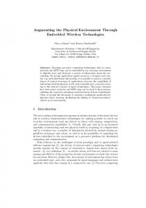
Fig. 1. Example of the transformations performed by αk,h and γk,h .
where ℘(X) is the powerset of X, ⊤⊆ = C1+ , ⊥⊆ = ∅, (C1+ )2⊥ = (C1+ ×C1+ )∪{⊥≺ }, ⊤≺ = (f⊥≺˙ : x 7→ −∞, f⊤≺˙ : x 7→ +∞), f1 ∨f2 = f such that ∀x ∈ R+ , f (x) = f1 (x) if f1 (x) ≥ f2 (x) and f (x) = f2 (x) otherwise. ∧ is defined in the same way. Note that for all f1 ∈ C1+ , f2 ∈ C1+ , f1 ∨ f2 ∈ C1+ and f1 ∧ f2 ∈ C1+ . α0 (X) = (f − , f + ) such that ∀x ∈ R+ , f − (x) = inf {f (x) : f ∈ X} and + f (x) = sup {f (x) : f ∈ X}. For all X ⊆ C1+ , α0 computes functions belonging to C1+ , at least if, in T0 , we restrict ourselves to families of functions F for which {x : ∃f ∈ F, the derivative of f is discontinuous in x} is finite (we believe that ˙ ≺f ˙ + }. this assumption can be relaxed). γ0 (f − , f + ) = {f ∈ C1+ : f − ≺f In a static analyzer, the user ought to specify the continuous inputs as values of T1 , i.e. as pairs of functions that the tool will numerically approximate. The second abstraction, introduced now, defines how safe approximations of sets of functions should be computed by the analyzer. Basically f − and f + are conservatively approximated by step functions, (see Figure 1). Let F be a set of floating-point numbers and let E+ denote the set of step functions e : R+ → F. γk,h
−− −−− − hE+ × E+ , ≺, ∨, ∧, ⊤≺ , ⊥≺ i = T2 T1 = h(C1+ )2⊥ , ≺, ∨, ∧, ⊤≺ , ⊥≺ i ← −− → α −− k,h
(2)
k is a positive integer and h is a positive floating-point number. αk,h (f − , f + ) = + − + (α− k,h (f ), αk,h (f )) such that: − − α− : ∀i : 0 ≤ i < k, ∀t : ih ≤ t < (i + 1)h, e− (t) ≤ f − (t) k,h (f ) = e
(3)
+ + α+ : ∀i : 0 ≤ i < k, ∀t : ih ≤ t < (i + 1)h, e+ (t) ≥ f + (t) k,h (f ) = e
(4)
∀t ≥ kh, e− (t) ≤ f − (t) and e+ (t) ≥ f + (t)
(5)
α− k,h
α+ k,h ,
Equations (3-5) do not indicate how to compute and but any implementation that conforms to these conditions is a correct abstraction. We believe + that standard numerical algorithms can be adapted to compute α− k,h and αk,h . For instance, for functions of T1 defined by differential equations, the first k steps of e− and e+ could be computed using a Runge-Kutta method, and using the IEEE Standard 754 rounding modes towards −∞ for e− and towards +∞ for e+ [2]. For the last step, corresponding to time t ≥ kh, safe approximations can also be computed. For example, if f − and f + belong to C2+ (their first derivative is piecewise smooth) the sign of their second derivative may help to find a fine approximation. Interesting abstractions could also be designed for periodic functions (e.g. in Fourier’s space), like the trigonometric functions, which
often correspond to realistic physical inputs of digital signal processing algorithms used in embedded software [10]. In addition, for k ′ > k, αk′ ,h is a finer abstraction than αk,h . A similar property holds for h. γk,h has to compute a pair of functions of C1+ but, e.g., ∨{f ∈ C1+ : f ≺ + e } 6∈ C1+ . We have to perform an additional approximation and to chose, for + example, to let γk,h (e+ ) be a linear interpolation function linking the points + (ih, e (ih)) to ((i + 1)h, e+ ((i + 1)h)), for 0 ≤ i < k, as shown in Figure 1.
3
A Simple Analysis
Computer calculations are carried out using floating-point numbers that introduce roundoff errors. For critical embedded systems, a major safety property should consist of proving that programs take the same decisions than ideal systems working with real numbers. Let p be a program whose inputs are given by sensors corresponding to volatile variables x1 , . . . , xn . For 1 ≤ i ≤ n, Fi ⊆ ℘(C1+ ) is a set of possible concrete functions modeling the sensor related to xi . [[p]]R and [[p]]F denote the collecting semantics of p in which calculations are carried out with real number and floating-point numbers, respectively. We wish to compare the traces of [[p]]R (F1 , . . . , Fn ) and [[p]]F (F1♯ , . . . , Fn♯ ), where Fi♯ = α0 ◦ αk,h (Fi ), 1 ≤ i ≤ n. We assume that loops are precisely cadenced, that is that we know how long lasts an iteration. This is usually known since embedded software are real-time programs for which the designer knows, e.g. that some loop runs at x Hz. So we have at least a precise interval of time to date each point of an execution trace. WCET tools also finely compute this information [5]. To perform our analysis, we define a simple concrete semantics [[.]] in which a value is a pair of F × R written v = f εf + eεe . εf and εe are formal variables. This semantics, detailed in [11], is a special case of a family of more informative semantics [9]. For example, for v1 = f1 εf + e1 εe and v2 = f2 εf + e2 εe , the sum is defined by [[v1 + v2 ]] =↑◦ (f1 + f2 )εf + [e1 + e2 + ↓◦ (f1 + f2 )]. For x ∈ R, ↑◦ (x) ∈ F is the roundoff of x and ↓◦ (x) = x− ↑◦ (x) ∈ R. In the abstract semantics [[.]]♯ related to [[.]], the values are made of pairs of IF × IMP , i.e. an interval of floating-point numbers and an interval of multiple precision floatingpoint numbers closely approximating a set of real numbers. We can now define the abstract semantics of a volatile variable xi in the time interval [t, t′ ]: [[xi ]]♯ = [a, b]εf + [−u, u]εe
Fi♯
(Fi−♯ , Fi+♯ ),
min(Fi−♯ ([t, t′ ])),
(6)
max(Fi+♯ ([t, t′ ])),
with = a = b = and u = max(ulp(|a|), ulp(|b|)). ulp(x) is the unit in the last place of x [7]. The analysis defined by [[.]]♯ allows one to detect divergences of control flow between [[.]]R and [[.]]F , that is to detect different decisions taken by an ideal program and its implementation. For a value v = f εf +eεe of [[.]]♯ , they correspond to conditions cond(v) for which [[cond(v)]]F = cond(f ) 6= cond(f + e) = [[cond(v)]]R .
4
Future Work
First of all, the analysis of Section 3 is too simple to be useful in practice. Indeed, “small” divergences of control flow between [[.]]R and [[.]]F are common
and admitted. However, [[.]]♯ shows how we technically plan to address more interesting problems. To allow “small” divergences of control flow, the safety property expressed in Section 3 should be reformulated as “given a program which, in [[.]]R , reaches some control point between the instants t and t′ , when does the same program, in [[.]]F , reach the same control point?”. For example, if an alarm must be raised when the value of a sensor reaches a certain threshold at time t, we wish the implementation raise the same alarm in an acceptable delay around t and we want to bound this delay. Secondly, as discussed in Section 2, conservative algorithms computing safe approximations αk,h satisfying the correctness criteria of equations (3-5) have to be designed. Next, we want to add the interactions from programs to their environment (actuators). This makes the continuous functions related to the volatile variables change dynamically, significantly complicating the analysis. Finally, software for embedded systems often are concurrent programs interacting together by classical communications between computer programs but also via their actions on the shared physical environment. We also plan to extend our work to the case of concurrent systems.
References 1. R. Alur, C. Courcoubetis, N. Halbwachs, T. A. Henzinger, P.-H. Ho, X. Nicollin, A. Olivero, J. Sifakis, and S. Yovine. The algorithmic analysis of hybrid systems. Theoretical Computer Science, 138, 1995. 2. ANSI/IEEE. IEEE Standard for Binary Floating-point Arithmetic, 1985. 3. P. Cousot and R. Cousot. Abstract interpretation: a unified lattice model for static anal ysis of programs by construction or approximation of fixpoints. In POPL’77, pages 238–252. ACM Press, 1977. 4. Blondel V. et al. Deciding stability and mortality of piecewise affine dynamical systems. Theoretical Computer Science, 255, 2001. 5. C. Ferdinand, R. Heckmann, M. Langenbach, F. Martin, M. Schmidt, H. Theiling, S. Thesing, and R. Wilhelm. Reliable and precise wcet determination for a real-life processor. In EMSOFT’01, number 2211 in LNCS. Springer Verlag, 2001. 6. J. Feret. Static analysis of digital filters. In ESOP’04, number 2986 in LNCS, pages 33–48. Springer-Verlag, 2004. 7. D. Goldberg. What every computer scientist should know about floating-point arithmetic. ACM Computing Surveys, 23(1), 1991. 8. N. Halbwachs, P Raymond, and Y.-E. Proy. Verification of linear hybrid systemss by means of convex approximations. In SAS’94, LNCS. Springer Verlag, 1994. 9. M. Martel. Propagation of roundoff errors in finite precision computations: a semantics approach. In ESOP’02, number 2305 in LNCS. Springer-Verlag, 2002. 10. M. Martel. Validation of assembler programs for dsps: A static analyzer. In PASTE’04. ACM Press, 2004. 11. M. Martel. An overview of semantics for the validation of numerical programs. In VMCAI’05, number 3385 in LNCS. Springer-Verlag, 2005. 12. P. J. Mosterman. An overview of hybrid simulation phenomena and their support by simulation packages. In Hybrid Systems: Computation and Control, LNCS, pages 165–177. Springer Verlag, 1999.