Towards an Evolutionary Tool for the Allocation of ... - CiteSeerX

Towards an Evolutionary Tool for the Allocation of Supermarket Shelf Space ∗

Anna I Esparcia-Alcazar ´ Lidia Lluch-Revert Ken C Sharman

Jose´ Miguel Albarrac´ın-Guillem Marta E Palmer-Gato

Instituto Tecnologico de Informatica ´ ´ Edif. 8G Acc. B, Ciudad Politecnica de la Innovacion ´ ´ 46022 Valencia, Spain

Departamento de Organizacion ´ de Empresas, Econ. Financiera y Contabilidad Universidad Politecnica de Valencia ´ Camino de Vera s/n 46022 Valencia, Spain

anna, lillure, [email protected]

jmalbarr, [email protected]

ABSTRACT

In [9] we can find an extensive literature survey of both exact methods and heuristics applied to the allocation of shelf space to each product, although the authors point out the lack of academic work on this subject. Also, the models found are complex and have practical limitations. Further, the simplifications used make retail application unrealistic. All these methods face the problem of incorporating real world cases, due to the existing complexity and the multitude of variables. In the real business case that we were presented with, however, the maximisation of the profit and the actual allocation of products to shelves were solved at different levels. At the top level, the management determine what are the optimal (profit-wise) lengths of shelves to allocate to each product, called the category standards. The set of category standards that configures a shop is termed the standard shop. At the lower level, the shop planners must take this “ideal” shop configuration and adapt it to the actual space available. Their objective is to allocate lengths of shelves to particular products, given a real shop layout and the standard shop requirements. The problem they face is the lack of suitable tools to achieve this. The aim of this paper is to present an evolutionary tool that can precisely do this. On the one hand, the method can handle realistic problems (both in terms of size and complexity); on the other, it is at the same time operationally viable, in that it can provide results within reasonable timescales. At the same time, the tool can provide solutions that are easily understandable to the shop planner. The paper is laid out as follows. In Section 2 the problem is described, together with the exact and evolutionary approaches to address it. In Section 3 the experiments are detailed and Section 4 summarises the conclusions and further work.

In this paper we set the first steps towards the development of a commercially viable tool that uses evolutionary computation to address the Product to Shelf Allocation Problem (P2SAP). The problem is described as that of finding the numbers and locations of modules to allocate to particular products in a shop, fulfilling at the same time a number of constraints. We first justify the use of evolutionary algorithms in this problem in the bad scalability properties shown by exact methods. Then we proceed, from simpler to more complex versions of the problem, to describe different encodings, fitness functions and evolutionary operators that are suited to the problem. The variations described are tested on five different problem configurations: three with one shelf, one with two shelves and one with eight shelves. In all cases acceptable results can be obtained in a very short timescale, although there is much work to be done on the subject. Categories and Subject Descriptors: F.2.2 [Theory of Computation]: Nonnumerical Algorithms and Problems General Terms: Algorithms. Keywords: Shelf-space allocation, evolutionary algorithms.

1. INTRODUCTION The problem of allocating space to a particular product in a shop is typically addressed in the literature as that of deciding what combination of products will yield the maximum profit. In general, the most commonly employed methods try and measure the impact on the customer of the relationship between allocated space and sales [1][2][5][7]. The aim is to find the allocation of space that maximises the profit. ∗Corresponding author.

2. Permission to make digital or hard copies of all or part of this work for personal or classroom use is granted without fee provided that copies are not made or distributed for profit or commercial advantage and that copies bear this notice and the full citation on the first page. To copy otherwise, to republish, to post on servers or to redistribute to lists, requires prior specific permission and/or a fee. GECCO’06, July 8–12, 2006, Seattle, Washington, USA. Copyright 2006 ACM 1-59593-186-4/06/0007 ...$5.00.

2.1

THE PRODUCT TO SHELF ALLOCATION PROBLEM (P2SAP) Problem description

In this paper we will concentrate on finding actual values of lengths per product that are close enough to the ideal values, and locating them so as to fulfill other requirements. This we refer to as the Product to Shelf Allocation Problem (P2SAP), to distinguish it from the Shelf-Space Allo-

1653

cation Problem (SSAP) described in [9]. The P2SAP that we describe here arose as part of the expansion process of a Spanish supermarket chain, whose managers were interested in opening a significant number of new supermarkets in a short period of time. When a new store is opened, the shop planners are given the standard shop requirements. In practice, this is a list of all categories (or products) plus their corresponding category standards. A shelf is divided into modules of given length, so the category standard can be expressed as a length in metres or as an integer number of modules, with a minimum of one. Some categories can also have a specification of number of modules by which their category standard can be increased or decreased if necessary. Because the size and layout of different premises can vary, the standard shop requirements cannot be fulfilled exactly, so for some categories the number of allocated modules have to be increased or decreased. There are also other constraints for the placing of categories. Firstly, categories are classified into groups (e.g., baby milk belongs to the generic group of baby products) so categories in the same group must be placed together. Groups should be kept as cohesive as possible; it does not make sense to put a module containing tinned beans at the end of a shelf full of toiletries, only because that is what the standard number of modules for that category specifies. Next, categories and groups can have affinities or disparities between them. For instance, baby products are disparate, or adverse, to pet food because, seemingly, customers do not like seeing the two things together. Groups containing food products are affine to each other, but indifferent to housewares. Finally, some groups must be placed near reference points. For instance, bakery products must be placed near the oven (even though they are not manufactured in store) or expensive spirits must be placed near the checkouts, so that the cashiers can keep an eye on them. With all these constraints and the standard shop requirements, the shop planner can take several days to come up (by hand) with a layout for the new shop. If many shops have to be opened at the same time, this is not acceptable. Also, for existing shops, there is the problem of new categories being introduced everyday, which implies frequent reorganisation.

1 std1 min1 max1 p1 B std2 min2 max2 p2 C SS = B .. .. .. .. C @ A . . . . stdK minK maxK pK 0

(1)

where stdi , mini and maxi are the standard, minimum and maximum number of modules to allocate to unit i, respectively, (where a unit can be a category or a group) and pi is the preference for the increase in modules • Affinity constraints. We will represent these by a K × K affinity matrix, A, where each component ai,j denotes the affinity between categories i and j, as follows: 8 > :> 0 if c and c are affine i j • Location with respect to reference points

• Group cohesion. This and the previous one are softer constraints and we will see how to handle them below. The first two constraints relate to the number of modules to allocate to each category, while the last three relate to their relative position. So we have a dual objective to achieve: on the one hand, to find the “ideal” number of modules (as opposed to the “standard” number); on the other hand, to find the ideal allocation of categories to the modules. However, in this first approach to the problem we will use a simple heuristic to attain the first objective and will concentrate on the second objective. For this we will need a further definition: an M × M distance matrix, D, where each component di,j denotes the distance between units i and j, where a unit can be either a category, a module or a group, depending on the problem configuration.

2.3

Exact approaches to the P2SAP

The first approach we can take to this problem is the complete enumeration of the solutions. Since essentially what we are looking for is a permutation of the K categories, we can find an algorithm that generates all the possible K! permutations, evaluates them and chooses the best. However, this is only feasible for really small versions of the problem. For K = 16 and assuming a time of 1µs per operation, just generating the solutions would take 8 months; for K = 17 the time would be above 10 years. A second approach to the P2SAP is to model it as a Mixed Integer Quadratic Assignment Problem (MIQAP) using an objective function as follows:

2.2 Definitions Given a set of K categories (or products) that can be grouped into a set of G groups, and a set of S shelves, each one divided into Mi , i = 1, . . . , S modules, with the total s P Mi ≥ K. number of modules M = i=1

The P2SAP consists of finding a matrix X representing an allocation of categories to modules, ( 1 if category ci is assigned to module mk xi,k = 0 otherwise

f=

K K M M 1 XXXX aij · dkl · xik · xjl , 2 i=1 j=1

j > i,

k 6= l (2)

k=1 l=1

subject to the following constraints:

The aim is to find combinations of the xik and xjl that minimise f , subject to the constraints shown above. In our experiments, for a simple problem (S = 1, M = 10, K = 5) a solution was obtained in a few minutes. However, for a more complex problem (S = 1, M = 17, K = 10) the run time was of the order of 30 to 40 hours. For even more complex problems we could not obtain a solution with the

• Space available. This is a hard constraint that can be represented as K P M P xi,u = M i=1 u=1

• Standard shop requirements. We will capture these in a matrix as follows

1654

Parameters of the evolutionary algorithm Population size 100 (P2SAP1), 200 (P2SAP2), 400 (P2SAPn) Selection method Tournament Tournament size 5 (P2SAP1 & 2), 10 (P2SAPn) Mutation probability 1/chromLength Diversity preservation Restart + seeding with best mechanism when 80% individuals are equal

software employed1 . In view of these figures and given that, according to [10], an average supermarket of medium size has between 5000 and 7000 categories, it seems obvious that a different approach to their allocation must be taken. The choice was an evolutionary approach.

2.4 The evolutionary approach to the P2SAP For simplicity reasons we decided not work with the matrix X and tried different codings instead. The coding varied with each problem configuration and will be explained below. The same goes for the fitness function employed. The evolutionary process started by generating a random population of individuals or chromosomes representing solutions to the problem at hand. Then evolution proceeded employing the following operators:

Table 1: Parameters of the evolutionary algorithm employed in the experiments. The values of the population and tournament sizes were chosen after experimentation. Following [6], the mutation probability equals the inverse of the chromosome length.

• reOrderXover : This is a variant of the standard crossover operator used when the chromosomes are permutations of a series of natural numbers and therefore each number can appear only once. Two parents are selected. The genes (components) of each parent are reordered from the (random) crossover point in the same order as they appear in the other parent.

component i stores the category allocated to module i. Since M = K we always have a one-to-one correspondence between modules and categories. We considered modules of unit length and defined the distance between two consecutive modules as equal to 1. The fitness function was defined as follows:

• swap : The values of two genes selected at random in a chromosome are swapped

K K 1 XX (di,j · |ai,j |)sgn(ai,j ) 2 i=1 j=1

f=

• shift(n) : The genes in a chromosome are shifted n (a random value) positions to the left if n < 0 or to the right if n > 0

where di,j ai,j

• shuffle(n): Given a random number n, select randomly a segment of n genes within the chromosome and shuffle their values.

(3)

is the distance between modules mi and mj is the affinity between the categories allocated to modules mi and mj ( sign(ai,j ) ∀ai,j 6= 0 = 0 ai,j = 0

sgn(ai,j )

3. EXPERIMENTS

and the objective was to minimise f . We took M = K = 10 and used a randomly generated affinity matrix, as follows

3.1 One shelf - P2SAP1 This is the simplest version of the problem. We considered three variants: • P2SAP1.1 - The number of modules equals the number of categories (M = K)

0

B B B B B A=B B B B B @

• P2SAP1.2 - The number of modules is greater than the number of categories (M > K) • P2SAP1.3 - As P2SAP1.2, but with a reference point As said above, we did not work with the matrix X, but rather collapsed it into a single vector chrom, the chromosome or individual. In general the chromosomes are vectors of natural numbers which in the simpler versions of the problem represent the categories.

− 1 -1 0 0 1 1 0 -1 1

1 − 0 0 1 1 1 -1 0 1

-1 0 − 1 0 1 -1 0 1 -1

0 0 1 − -1 -1 -1 0 -1 -1

0 1 0 -1 − -1 1 0 1 0

1 1 1 -1 -1 − 0 1 0 -1

1 1 -1 -1 1 0 − 1 1 -1

0 -1 0 0 0 1 1 − 1 0

-1 0 1 -1 1 0 1 1 − 1

1 1 -1 -1 0 -1 -1 0 1 −

This means that c1 c2 c3 c4

P2SAP1.1 For this simple case we did not consider groups, or rather, we assumed that each category belongs to its own group. To represent affinities between categories, the components of A will take values of 1, −1 or 0. We implemented an evolutionary algorithm in which the chromosomes are coded as vectors of length M where each

is is is is

affine affine affine affine

to to to to

1 C C C C C C C C C C A

c2 , c6 , c7 and c10 and adverse to c3 and c9 c1 , c5 , c6 , c7 and c10 and adverse to c8 c4 , c6 , and c9 and adverse to c1 , c7 and c10 c3 and adverse to c5 , c6 , c7 , c9 and c10

and so on. We ran the evolutionary algorithm 20 times. After 3 seconds, the best result obtained was always: chrom =

`

4 3 6 8

or its symmetric: ` chrom = 1 10 2 5

1

CPLEX version 9.1 running on a Pentium IV 3.0 GHz with 1 GB RAM.

1655

9 7 5 2 10

1

´

7 9 8 6 3

4

´

NO Initialise Population

Evaluate Population

Check diversity?

Iters=0

Tournament selection

NO

YES

NO

Mutate offspring with Pm

Crossover

Tsize individuals

Evaluate offspring

Reinsert individuals

2 individuals

Diversity is low?

Termination criterion? Iters++ Best chromosome

Restart + Seeding

YES

YES

Figure 1: The evolutionary algorithm employed in the experiments

resulting in a shelf layout as follows: c4

c3

c6

c8

c9

c7

c5

c2

c10

c1

c3

c4

0

B B B B SS = B B B @

or, conversely, c1

c10

c2

c5

c7

c9

c8

c6

Analysing the result, we can see that c4 , which is adverse to 4 categories, is placed at the end of the shelf, next to the only other category it is affine to. In other cases, compromises must be reached. This is for instance the case of c6 , which wants to be close to c3 but far from c4 . We must point out that the affinity matrix was obtained at random and in reality this kind of situation may not arise because there are not so many affinities and disparities between categories, most of them being indifferent to one other.

5 1 2 4 7 8 3 6

1 1 1 1 1 1 1 1

4 4 4 4 4 4 4 4

1 C C C C C C C A

(4)

where the first column has been omitted because it was not used. Hence, categories c6 and c5 have the highest preference and c2 and c3 the lowest. According to the highest averages method, the allocation of modules to categories would then be a vector h as follows: ` ´ h= 1 1 1 1 2 2 1 1 meaning all categories get allocated one module, except c5 and c6 , which get two. The affinity values will be given by 8 −1 if ci and cj belong to adverse groups > > > > 0 if ci and cj belong to indifferent groups > > < 1 if ci and cj belong to affine groups ai,j = 2 if ci and cj belong to the same group > > > > 3 if ci and cj belong to the same group > > : and are affine to each other

P2SAP1.2 When M > K we must also allocate the number of modules that correspond to each category and not only their position. This will be given by an allocation vector, h. In order to calculate h in a way that satisfies the requirements of the standard shop, we will employ the category standards (or standard shop) matrix SS defined in Equation 1. In particular, we will work with the last three columns of this matrix. The last column defines the preference of each category, the highest value corresponding to the category of highest preference (i.e., the one that should be allocated more modules). The second and third columns specify the minimum and maximum number of modules per category respectively. The allocation procedure is as follows. First of all, we allocate the minimum number of modules to each category. Next we allocate the remaining modules using a variant of the highest averages method (or d’Hondt method2 ). The first spare module is allocated to the category with the highest preference. In the next round, the category that was allocated a module gets its preference divided by 2. In general, if a category has been allocated n spare modules, its preference to get the next one (assuming its maximum has p0 , where p0 is the initial preference. not been reached) is n+1 The process ends when all the spare modules have been allocated. For our experiments we used M = 10 and K = 8 and a category standard matrix as follows:

We chose the following combination of groups: g1 : g2 : g3 :

categories c1 , c2 , c3 and c4 categories c5 and c6 categories c7 and c8

where groups g1 and g2 are adverse; group g3 is indifferent to g2 and affine to g1 . Within group g1 , categories c1 and c3 are affine and the rest are indifferent. This results in an affinity matrix as follows: 0

B B B B A=B B B @

− 2 3 2 -1 -1 1 1

2 − 2 2 -1 -1 1 1

3 2 − 2 -1 -1 1 1

2 2 2 − -1 -1 1 1

-1 -1 -1 -1 − 2 0 0

-1 -1 -1 -1 2 − 0 0

1 1 1 1 0 0 − 2

1 1 1 1 0 0 2 −

1 C C C C C C C A

(5)

The chromosome is encoded as a vector whose length equals the number of categories, but in this case this is not the same as the number of modules. The chromosome indicates the order of the categories in the shelf and we will use the allocation vector given by the highest averages method to determine the layout of the actual shelf.

2 This method is named after 19th century Belgian mathematician Victor d’Hondt and is used in the European Union, as well as several European countries, for the allocation of seats in parliament; see, for instance, [4].

1656

We ran the experiment 80 times with a population size of 100 and a tournament size of 5. The run time was 60 seconds, but typically within two seconds a minimum fitness of 52.5845 was reached. This corresponds to 32 similar solutions, some of which are given here: ” “ chrom = 6 5 8 7 2 3 1 4 “ ” chrom = 5 6 7 8 1 3 2 4 ” “ chrom = 4 3 1 2 8 7 6 5 “ ” chrom = 4 2 3 1 8 7 6 5

rence matrix as given by Equation 4, the highest averages algorithm provides a module allocation h as follows: ` ´ h= 3 1 2 3 3 3 2 3

which means c2 gets one module, c3 and c7 get 2 modules each and the rest get 3 modules each. We ran the evolutionary algorithm 30 times with a population size of 100 and a tournament size of 5. The run time was 15 seconds (increasing the time does not provide better results). When the diversity is low (80% of individuals are the same), the population is reinitialised and seeded with the best result so far (see Figure 1). The best results obtained were as follows: ` ´ 0 8 7 4 2 3 1 6 5 chrom = ` ´ 0 8 7 4 2 3 1 5 6 chrom =

where we have boxed those categories belonging to the same group to show that the algorithm has placed them together. Also, categories c1 and c3 are next to each other in all the solutions, groups g1 and g2 are always apart and groups g1 and g3 are always together.

the former resulting in an actual shelf layout as follows:

c8 c8 c8 c7 c7 c4 c4 c4 c2 c3 c3 c1 c1 c1 c6 c6 c6 c5 c5 c5 with categories c7 and c8 placed next to the header of the shelf, as was required. For M = 20 and K = 10 we add two extra categories, c9 and c10 , to group g3 . The category standards matrix was the same as in Equation 4 adding two rows at the end to represent that c9 and c10 have now the highest preference. This gives a module allocation vector h of : ` ´ h= 2 1 1 2 2 3 1 2 3 3

The actual shelf layout corresponding to, say, the first solution, given the allocation of modules to categories obtained by the highest averages algorithm, would be as follows: c6

c6

c5

c5

c8

c7

c2

c3

c1

c4

i.e. there are two modules for categories c5 and c6 and one for the rest.

The affinity matrix was modified adding two new rows and columns for the new categories, but also the affinity values of c7 and c8 to the reference point were increased to 3. The best results obtained after 50 runs were ` ´ 0 8 7 9 10 2 3 1 4 6 5 chrom = ` ´ 0 8 7 10 9 2 3 1 4 6 5 chrom =

It is worth noticing that the problem could be greatly simplified if instead of placing the categories we concentrated on placing the groups. We will make use of this idea later on. P2SAP1.3 In this problem a reference point is introduced, which we will assume is placed at the header of the shelf, on the left hand side. We simulate this as a fictitious module, m0 , plus a fictitious category, c0 , that will always be placed in that module. We introduce an extra row and column in the affinity and distance matrices. The categories that must be close to the reference point will have an affinity value of 2 to the fictitious category. This is similar to the affinity value between categories belonging to the same group. The affinity matrix in this case was the same as in Equation 5 but modified adding one new row and column for the fictitious category. In these, all the values are zero except those corresponding to c7 and c8 , which equal 2, meaning categories c7 and c8 must be placed close to the reference point. 0

B B B B B A=B B B B @

− 0 0 0 0 0 0 2 2

0 − 2 3 2 -1 -1 1 1

0 2 − 2 2 -1 -1 1 1

0 3 2 − 2 -1 -1 1 1

0 2 2 2 − -1 -1 1 1

0 -1 -1 -1 -1 − 2 0 0

0 -1 -1 -1 -1 2 − 0 0

2 1 1 1 1 0 0 − 2

2 1 1 1 1 0 0 2 −

which differ only in the positions of c9 and c10 . The first one gives a shelf layout of: c8 c8 c7 c9 c9 c9 c10 c10 c10 c2 c3 c1 c1 c4 c4 c6 c6 c6 c5 c5 In this case, to keep categories c7 and c8 next to the header we had to increase their affinity to it, because keeping it as in the previous experiment did not achieve the desired result. This shows the sensitivity of the results to the selection of the affinity values.

3.2

Two shelves separated by an aisle - P2SAP2

We will consider now the case of two face-to-face shelves consisting of 10 and 13 modules of length 1 and separated by an aisle of width 3. There is also a reference point located at the left end of the aisle. The chromosome is now a vector consisting of two parts. The first S − 1 components indicate the number of categories to be placed in a shelf (with S equal to the number of shelves). The remaining components indicate the order in which the categories will be placed in the shelves. Hence the length of the chromosome will be S − 1 + K. For instance, let us assume S = 2 and K = 8. A chromosome such as:

1 C C C C C C C C C A

(6)

The problem can then be reduced to the previous case, with the restriction that c0 will always be located in m0 . For this example we chose M = 20 and two values of K, K = 8 and K = 10. For M = 20 and K = 8 and a prefe-

chrom =

`

3 8 5 1 3

2 6 4 7

´

indicates that there will be 3 categories in the first shelf (c8 , c5 and c1 ) and the remaining 5 (c3 , c2 , c6 , c4 , and c7 ) will

1657

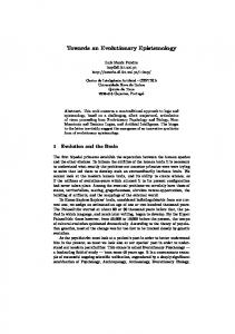
3.3

be placed in the second shelf. The vector h indicating the number of modules per category will be determined independently for each shelf following the highest averages method. We will also calculate a vector hg , which indicates the number of modules that would be allocated per category if all the modules were grouped in a single shelf, i.e., the global h. We will assume that:

We will address here the problem with a more complex topology: eight shelves in different positions, as shown in Figure 2. The approach we will take is to concentrate on the placing of groups instead of categories. This brings about two simplifications, namely: • The components of the affinity matrix can take one of three values: −1, 0 and 1.

• A category cannot be distributed over two shelves • It is preferable to place two affine categories on the same shelf rather than split into two shelves, even when the Euclidean distance between modules of different shelves is less than between modules of the same shelf.

• A group can be distributed over more than one shelf. As a consequence of the above, the matrices A, SS and D now refer to groups and not categories. So, ai,j and di,j are the affinity and distance, respectively, between groups gi and gj . And the columns of SS contain the standard, minimum and maximum number of modules per group. The distance between groups is going to be taken now as the distance between their centres of gravity. We define the centre of gravity (c.o.g.) of a group as the module in the group for which the sum of the distances of itself to every other module in the group is minimal; if several modules fulfill this condition then the first one encountered will be taken as the c.o.g. Another major difference between this and previous versions of the problem is that now the allocation of number of modules per group is going to be done as part of the evolutionary algorithm, rather than using a separate algorithm to calculate it. Also, because a group can be spread on different shelves, we must ensure that the group maintains sufficient cohesion, in other words, we have to control the group dispersion. We will introduce a different encoding for the chromosome. Instead of a vector, we will employ a MATLAB cell array structure, which is a matrix in which the rows can different lengths. In our case each row i stores the modules allocated to group gi . The restrictions are, as before, that the total number of elements must equal the total number of modules in the shop and that each chromosome represents a permutation of the modules’ indices. For instance, for G = 3 and M = 10 a possible chromosome would look like this:

After trying different variations of the fitness function, we settled for: K K ” 1 XX“ (di,j · |ai,j |)sgn(ai,j ) · pi,j +β·||hg −h||2 (7) f= 2 i=1 j=1 where di,j , ai,j and sgn(ai,j ) are as defined for Equation 3 the affinity matrix A is as for Equation 6 ||hg − h||2 is the quadratic distance between h and hg and the penalty, pi,j , is defined as follows 8 ( if ci and cj are on different shelves and ai,j > 0 > > < or if ci and cj are on the same shelf P pi,j = and ai,j < 0 > > :1 otherwise Different values of P and β were tried and finally we settled for P = 100 and β = 50. We run the algorithm 30 times, with a population size of 200 and a time limit of 50 seconds per run, obtaining the following best solutions ` ´ 2 5 6 7 8 2 3 1 4 chrom = ` ´ 2 5 6 8 7 2 3 1 4 chrom = ` ´ 2 6 5 7 8 2 3 1 4 chrom = ` ´ 2 6 5 8 7 2 3 1 4 chrom = with a value of h as follows: ` h= 3 1 1 3 5

while the value of hg is: ` hg = 3 1 2

5 2 3

´

3 4 4 3 3

´

0

9 7 chrom = @ 10 8 2 6

c5

c5

c5

c5

c6

c6

c6

c6

c6

c7

c8

c8

c8

c2

c3

c1

5 1 3 A 4

• group affinity,

AISLE c7

1

meaning group 1 gets modules 9 and 7, group 2 gets modules 1, 3, 5, 8 and 10, and so on. When defining the fitness function we must take into account three different objectives:

which differs from h in four values. The actual shelf layout for the first result is: c5

A more complex topology - P2SAPn

c1

c1

c4

c4

c4

• deviation from the standard shop in terms of number of modules, and

which achieves the objectives of • placing c7 and c8 close to the reference point (located in (0, 0), to the left of the shelves),

• dispersion of the modules belonging to a group.

• all categories belonging to the same group are together and on the same shelf • the allocation of modules is relatively close to the “ideal” obtained by the highest averages method

1658

The last two objectives are specific of this version of the problem. The dispersion refers to how far apart the modules allocated to a group are located. To measure this, we introduce two penalty coefficients in the evaluation function:

6

7

8

9

10

11

12

13

14

15

16

s2

5

A1

4

dispgi =

A2

3 2

26

25

24

23

22

21

20

19

18

17

1

27

28

29

30

31

32

33

34

35

36

s1

s3 s4

49

48

59

50

47

51

46

57

52

45

40

56

53

44

41

55

54

43

42

s7 s6

s5

58

A4

s8

37 38

A5

39

All other parameters of the evolutionary algorithm remained the same. For the experiments we defined six groups, g1 to g6 , and two reference points (located at the headers of the shelves), which were modeled as two extra groups, g7 and g8 . The affinity matrix (now storing group affinity values) was as follows: 0

B B B B A=B B B @

g g ” 1 XX“ (di,j · |ai,j |)sgn(ai,j ) · pi,j + 2 i=1 j=1

(8)

where: di,j is the distance between the centres of gravity of groups gi and gj ; ai,j is the affinity between groups gi and gj ;

pgi ,gj

− 0 0 -1 0 0 1 1

0 − 1 0 0 0 0 0

0 1 − 0 0 0 0 0

-1 0 0 − 0 0 0 0

0 0 0 0 − -1 0 0

0 0 0 0 -1 − 0 0

1 0 0 0 0 0 − 0

1 0 0 0 0 0 0 −

1 C C C C C C C A

(10)

In Equation 10 it can be seen that g1 is affine with groups g7 and g8 , i.e., it is preferable to place this group in the shelves closer to the reference points. The standard shop requirements (now referring to group standards rather than the category standards) employed in the experiments are given by Equation 11, where the last column of the matrix indicates that all the groups have the same preference. 0 1 6 5 9 1 6 6 6 1 B C B 6 4 8 1 C C SS = B (11) B 12 5 15 1 C @ 10 7 13 1 A 19 10 20 1

r=1

8 > > >

> > : 1

(9)

• Groups mutation: all the modules corresponding to two groups are exchanged

Notice how for this problem the module allocation vector h is given by the evolutionary algorithm and not calculated beforehand, as in previous Sections. The resulting fitness function is as follows:

dispgr + ||std − h||2

+ S gi + δ

i

12

• Modules mutation: two groups exchange a random number of modules

• Intra-group penalty, δ: to penalise the dispersion of the modules belonging to a group.

g X

Mg3

• Number of modules mutation: the number of modules of a group is increased or decreased

• Inter -group penalty, P : to penalise the situation in which modules belonging to the same group are located in different corridors, and

+

(coggi , mk )

Finally, evolutionary operators have also been modified to accommodate the new representation. The following mutation operators were implemented:

Figure 2: Shop layout for P2SAPn, with 5 aisles, 8 shelves and 60 modules; the numbers represent the module identifiers, mi . The dashed lines represent the accessible side of the shelf; the shaded areas represent shelf headers, used as reference points.

f=

k=1

Sgi is the number of different shelves occupied by gi Mgi is the number of modules allocated to gi δ penalizes disperse modules as follows: 8 < aisles and ai,j > 0 or > : if c.o.g.gi and c.o.g.gj are on the same aisle and ai,j < 0 otherwise

We ran the algorithm 50 times, with a termination criterion of 30,000 iterations (approximately 25 minutes per run). Most runs (78%) obtained good solutions; seven of them (14%) obtained the best chromosome:

||std − h||2 measures the difference between the number of modules per group assigned by the algorithm and that given by the first column of the standard shop matrix SS. It is calculated as a quadratic distance between vectors; PG i=1 dispgi is the total dispersion of the modules within all groups, where dispgi is calculated as follows:

0 B B B B @

1659

1 2 3 4 5 6 27 28 29 30 31 32 33 34 35 36 37 38 39 40 41 42 43 44 45 46 47 48 49 50 51 52 53 54 55 56 57 58 59 60 7 8 9 10 11 12 13 14 15 16 17 18 19 20 21 22 23 24 25 26

1 C C C C A

1 1 1 1 1 1

6

6

6

6

A1

6

6

6

6

6

6

1 1 1 1 1 1

A2 6 3

6 3

6 3

6 3

6 2

6 2

6 2

6 2

6 2

6 2

6

6

6

6

A1

A4

5 5 5 5 5 5

4 4 4 4 4 4

6

6

6

6

6

6 2

6 3

6 3

6 3

6 3

A2 6 2

6 2

6 2

6 2

A3 5 5 5 5 5 5

6

6 2 A3

A5

4 4 4 4 4 4

5 5 5 5 5 5

A4

5 5 5 5 5 5

4 4 4 4 4 4

A5

4 4 4 4 4 4

Figure 3: Allocation of groups to modules for two solutions of equal fitness

depicted in Figure 3, right, or a similar solution of equal fitness, depicted in Figure 3, left, in which groups 2 and 3 swap positions: 0 B B B B @

1 2 3 4 5 6 31 32 33 34 35 36 27 28 29 30 37 38 39 40 41 42 43 44 45 46 47 48 49 50 51 52 53 54 55 56 57 58 59 60 7 8 9 10 11 12 13 14 15 16 17 18 19 20 21 22 23 24 25 26

1 C C C C A

For both solutions the numbers of modules assigned to each group were: h = ( 6 6 4 12

12 20 )

5.

ACKNOWLEDGEMENT

This work was part of the ANaLog project and is supported by the Instituto de la Peque˜ na y Mediana Industria Valenciana (IMPIVA), N o Exp. IMCITA/2005/35, and partially funded by the European Regional Development Fund.

6.

REFERENCES

[1] Anderson, E.E., Amato, H.N.: A mathematical model for simultaneously determining the optimal brand collection and display area allocation, Operations Research, 22: 13-21 (1974) [2] Bai, R. and Kendall, G.: An investigation of automated planograms using a simulated annealing based hyper-heuristic. Automated Scheduling, Optimisation and Planning Research Group, School of Comp. Sci. and IT, Univ. of Nottingham. [3] Brijs, T., Swinnen, G., Vanhoof K. and Wets, G. Using association rules for product assortment decisions: a case study. Procs. 5th ACM SIGKDD Intl. Conf. on Knowledge Discovery and Data Mining, San Diego, USA, 254-260 (1999) [4] Corbett R., Jacobs F., Shackleton, M.: The European Parliament. London: John Harper (2001) [5] Corstjens, M., Doyle, P.: A model for optimizing retail space allocation, Management Science, 27(7): 822-833 (1981) [6] Eiben, A. E., Hinterding, R. and Michalewicz, Z.: Parameter control in Evolutionary Algorithms. IEEE Trans Evol Comp, 3: 124-141 (1999) [7] Hansen, P, Heinsbroek, H: Product selection and space allocation in supermarkets. Eur J Oper Res, 3:474-484 (1979) [8] Henderson, James B., Quandt, R.: Micro Economics Theory: a mathematical approach. New York: McGraw-Hill (1980) [9] Lim, A., Rodrigues, B. and Zhang, X.: Metaheuristics with local search techniques for retail shelf-space optimization. Management Science, 50(1):117-131 (2004) [10] Palomares, R.: Merchandising, c´ omo vender m´ as en establecimientos comerciales. Gesti´ on 2000, Barcelona. Pp. 127- (2001) [11] Shahidi, A.: The End of Supermarket Lethargy: Awakened Consumers and Select Innovators to Spur Change. Supermarket Industry Perspective (2002) [12] Walters, R.G.: Assessing the impact of retail price promotions on products substitution, complementary purchase, and interstore sales displacement. J. Marketing, 55(1):17-28 (1991)

which is “close enough” to the group standards, expressed in the first column of Equation 11: std’ = ( 6 6

• Employing an efficient algorithm to calculate the affinity matrix. Associating complementary products, because costumers need them at the same time to achieve a specific goal, is the most commonly employed method [3][8][11][12].

6 12 10 19 )

Notice the contribution to the result of the three components of the fitness function. First, the restrictions imposed by group affinities are accomplished: group 1 is close to the reference points, groups 2 and 3 are close to each other and groups 1 and 4 apart from each other. Second, all the modules belonging to the same group are placed together (thus minimising the dispersion). And finally, the number of modules assigned to each group is similar to the standard values.

4. CONCLUSIONS AND FURTHER WORK We have shown that our evolutionary algorithm can be used as a time-efficient tool to obtain solutions for the P2SAP. Future work will involve: • More complex topologies with higher number of shelves and more reference points. • Studying the contribution of the different components of the fitness function; also considering the possibility of addressing the problem as multi-objective. • Selecting a unique representation that can be applied to all versions of the problem. Also, studying how to address it with Genetic Programming rather than a Genetic Algorithm.

1660