Towards Automatic Calibration of In-line Machine Processes David F. Nettleton1, Elodie Bugnicourt1, Christian Wasiak2, Alejandro Rosales1
•
Abstract—In this work, preliminary results are given for the modeling and calibration of two different industrial winding MIMO (Multiple Input Multiple Output) processes using machine learning techniques. In contrast to previous approaches which have typically used “black-box” linear statistical methods together with a definition of the mechanical behavior of the process, we use non-linear machine learning algorithms together with a “white-box” rule induction technique to create a supervised model of the fitting error between the expected and real force measures. The final objective is to build a precise model of the winding process in order to control de tension of the material being wound in the first case, and the friction of the material passing through the die, in the second case. Keywords—Calibration, Data Model, Industrial Winding, Machine Learning.
Our approach builds a model using (i) non-linear machine learning algorithms and (ii) a “white-box” rule induction technique to create a supervised model of the fitting error between the expected and real force measures. The final objective is to build a precise model of the winding process in order to control de tension of the material being wound in the first case, and the friction of the material passing through the die, in the second case. The paper is structured as follows: in Section II, the historical setup and dataset of Bastogne et al. [1] is used to model the tension control of a winding process setup using two machine learning techniques; in Section III the Openmind H2020 project is briefly introduced; in Section IV the friction force control of a Micro-Pull winding process is modeled using three different machine learning techniques; Section V summarizes the current work.
I. INTRODUCTION
P
and pull winding are common in many industrial manufacturing systems. Pultrusion is a continuous manufacturing process for composite profiles which fuses multiple fiber threads using different resin systems to obtain the desired properties. Pull winding technology, on the other hand, makes it possible to obtain an accurate control of crosswise and longitudinal properties of a composite by varying the amount of fibers lengthwise and crosswise. However, these processes are susceptible to stochastic behaviors which can affect the quality of the final product. For example, slipping or distortion of the material during pulling which affects the tension, or build up of resin on the forming dies which affects the friction force. In this paper we use machine learning techniques to model the behavior of two different processes, and then apply a calibration step to find the optimal parameters which keep the system within allowed tolerances. • Previous approaches typically used “black-box” linear statistical methods together with a definition of the mechanical behavior of the process. ULTRUSION
1 David F. Nettleton, Elodie Bugnicourt and Alejandro Rosales are with IRIS SPAIN, Parc Mediterrani de la Tecnologia, Avda. Carl Friedrich Gauss nº 11, 08860 Castelldefels (Barcelona) - Spain (phone: + 34 93 554 25 00; fax: + 34 93 554 25 11; e-mails:
[email protected],
[email protected],
[email protected]). 2 Christian Wasiak is with Fraunhofer Institute for Production Technology IPT, Steinbachstr. 17, 52074 Aachen, Germany, (phone: +49 241 8904-0; fax: +49 241 8904-198; e-mail:
[email protected]). The Openmind project has received funding from the European Union’s Horizon 2020 research and innovation programme under grant agreement No 680820.
II. TENSION CONTROL OF A WINDING PROCESS This section follows the experimental setup defined by Bastogne et al. in [1] and the corresponding historical dataset [2]. This serves as a guide for the later Openmind data modeling, as it has been used by different authors in the state of the art. We apply a different approach to that of [1] in order to model the roving tension, benchmarking the SVR [3] and KRR [4] machine learning algorithms. A. Experimental Setup With reference to Fig. 1, a plastic web is unwound from a first reel, goes over a traction reel and is rewound on a third reel. The system to be modeled has five inputs (angular speed of reels 1, 2 and 3; setpoint current of motors 1 and 2) and two outputs (tension of material between reels 1 and 2; tension in material between reels 2 and 3) The objectives are to train a model to predict the tension based on the inputs and a calibration step to find the input values which result in a given tension.
Fig. 1. Schematic representation of the winding machinery. Source: [3] A desktop computer was used for all data processing with an Intel i5 processor, quad core, 8Gb RAM. The dataset consists of 2500 records of a winding process. From this data, two models are trained, one for each output: • Model 1: inputs u1 to u5 and output y1 • Model 2: inputs u1 to u5 and output y2 Then both models are put in a loop, assigning y1= value 1 and y2= value 2 as the objective outputs, in order to find the values of inputs u1 to u5 which give the closest fit of { y1', y2' } to { y1, y2 }.
B. Machine Learning Techniques: Kernel Ridge Regression and Support Vector Regression The data models were trained using the KRR_TRAINER and SVR_TRAINER from the Dlib C++ API function library[5]. Kernel Ridge Regression and Support Vector Regression are techniques described in refs. [4] and [3], respectively. Then a Gaussian random number generator was used to calibrate the inputs to some desired output(s) using the ‘Monte Carlo’ approach [6]. This is done specifying the desired mean and standard deviation for each input and then generating random input values with a Gaussian distribution until the model gives the desired output within a given tolerance. Tables I and II show the results for the KRR and SVR machine learning algorithms, respectively. The first two columns of Tables I and II show the target outputs for each data model, columns 3 to 7 show the inputs which are the same for both models; column 8 shows the modeling error on the output, which is measured as the sum of the distances between the target outputs and the real outputs. Table II has a slightly different format, as three different parameter settings were tested for the SVR algorithm. The parameter settings are indicated in rows 1, 3 and 8, with the corresponding results given in rows 2, 4 to 7 and 9, respectively.
TABLE I CALIBRATION RESULTS USING KERNEL RIDGE REGRESSION AS THE MODELING TECHNIQUE AND GAUSSIAN GENERATORS AS INPUTS Best combination of inputs found for Outputs targets Target Target i0 i1 i2 i3 i4 Dist1 2 ance -0.500 -0.500 1.295 0.809 0.650 1.106 -0.924 0.004 0.000 0.000 -1.711 1.518 -0.728 0.847 1.197 0.000 0.000 -0.500 -0.520 0.206 -0.856 0.514 -0.171 0.002 -0.500 0.000 -0.106 -0.205 0.162 -0.129 -2.065 0.000 -1.000 0.000 -0.073 -0.185 1.178 0.399 0.175 0.003 0.000 -1.000 -0.397 0.694 -1.128 1.999 -0.912 0.005 0.000 0.500 0.534 1.100 -0.153 0.155 0.989 0.001 0.500 0.000 0.295 1.056 -1.125 0.389 0.795 0.003 0.500 0.500 0.440 0.486 -0.616 -0.325 0.691 0.004 1.000 1.000 -0.734 0.952 0.655 -0.876 0.673 0.010 1.500 1.500 -0.561 -0.407 -0.852 -0.964 1.139 0.468 2.000 2.000 -0.759 -0.620 -0.879 -0.927 0.980 1.315 TABLE II CALIBRATION RESULTS USING SUPPORT VECTOR REGRESSION AS THE MODELING TECHNIQUE AND GAUSSIAN GENERATORS AS INPUTS Best combination of inputs found for Outputs targets Target Target i0 i1 i2 i3 i4 Dist1 2 ance using default parameter settings 0.5 0.0 -0.840 0.411 1.915 2.075 0.290 0.010 using custom parameter settings: c = range of output value; epsilon = desired precision x 10 0.5 0.0 -0.571 0.812 -0.260 0.304 0.621 0.007 0.5 0.0 -1.600 -0.375 -1.107 -0.327 0.739 0.003 0.5 0.0 -1.574 -0.350 0.168 0.365 -1.289 0.002 0.0 0.0 0.578 -0.448 -0.342 0.773 0.333 0.002 using custom parameter settings: c = range of output; epsilon = desired precision x 100 0.5 0.0 -0.374 -0.321 -0.423 0.313 0.128 0.003
C. Observations Processing speed and precision: a maximum of 100k iterations took 20 seconds on desktop computer (Intel i5 processor, quad core, 8Gb RAM), finding a best fit with error margin of 5x10⁻³. Note that this is with two outputs. For three or more outputs, the computational cost increase would probably be non-lineal, and the fit error could be significantly higher (maybe no model can be found for the given quality/error requirement). This dataset [2] has quite a good correlation between inputs and outputs: • Model 1: avg. correlation u1 to u5 with y1 = 65% ; avg. precision of model 69% (10 fold cross validation) • Model 2: avg. correlation u1 to u5 with y2 = 65% ; avg. precision of model 68% (10 fold cross validation) So this gives an idea of the data quality we need in order to build a model to obtain the cited fit and error. The results are promising, using an initial simple "brute force" approach and short cut-off time.
III. OPENMIND PROJECT Openmind [7] is a three year European H2020 project, counting with the participation of 9 Partners, including highly specialized industrial companies such as IRIS Advanced Engineering [8] and the Fraunhofer Institute for Production Technology IPT [9].
Project scope: the project considers the development of a highly flexible process chain for the on-demand production of entirely customized minimally invasive medical devices. This will enable even the production of small batch in a continuous, automated and fully monitored process.
Fig. 2. Schematic representation of the Openmind project
Openmind data flow scheme: The main tasks involve (i) integration and flexibilization of all relevant process steps into
a continuous and fully automated process chain; and (ii) seamless monitoring of all steps and the feedback of the data into the process for optimization and process development.
Fig. 3. Openmind data flow scheme
Future Openmind production line – advantages and challenges: Among the advantages, there will be the seamless chaining of formerly separated processing steps and achieving a combination of efficiency (continuous manufacturing) and flexibility (adaptive modules). Among the challenges there will
be machining in a running process, adaptation of processes for FRP micro profiles, obtaining a deep understanding and process modelling of linked processes and process control and quality management issues.
Fig. 4. Future Openmind production line
Fig. 5. Schematic pull winding process
A. IRIS’ work in Openmind project[7,8] IRIS has three main tasks in the Openmind project, related to the data modeling: (i) Concept of automatic parameter selection. This involves defining a methodological basis for software algorithms and methods used for the automatic parameter determination. Based on the whole process setup, a process model and all inputs of each process step will be designed that may vary for the manufacturing of a personalized product. (ii) Set of algorithms. Based on concept of automatic parameter selection, the most suitable algorithms and methods are identified and benchmarked for software development. (iii) Software for parameter selection. Supports machine operator to drastically simplify and accelerate the process development. This deliverable comprises the software itself, which will be fully integrated into the process chain, can handle all possible kinds of product and process variations, and can automatically deliver the best process setup for a specifically requested personalized product. IV. FRICTION FORCE CONTROL OF A MICRO-PULL WINDING PROCESS
This Section uses a pull winding dataset supplied by the Fraunhofer Institute [9] as part of the Openmind project [7]. The objective is to model the process using the friction force on the
second die as the output. We apply KRR [4] machine learning algorithms to model the data in subsections IV.E/IV.F and the M5Rules [10] algorithm to model the error in subsection IV.G. A. Experimental Setup A core together with a resin pass through a first die at a given temperature to cure the resin and fix the core strands. Next two winding units wind an outer layer around the core. This is followed by a new resin application and finally passing through a second die to cure and fix the outer windings. The two objectives are: (i) to train a model to predict the friction on die2 based on the following inputs: friction die1, temp die1 and die2, speed of winding units 1 and 2; and (ii) Calibration step: find the input values which result in a given friction on die2.
Fig. 6. Simplified schematic diagram of pull winding process
B. Data Modeling – Issues [11,12] The issues dealt with include: understanding the process hardware functionality and the data it generates; time lag processing; data normalization; understanding factors which
introduce deviation from expected behavior and modeling the corresponding error. C. Data Modeling – software and techniques used Two machine learning libraries/APIs were evaluated: Weka (Java) [13] and Dlib (C++) [5]. From these libraries, the following machine learning algorithms were evaluated: SVR (Support Vector Regression) with RBF (Radial Basis Function) Kernel; MLP (Multi-Layer Perceptron); MPART [10] (Rule induction with continuous value as output); Specific for time series KRLS (Kernel Recursive Least Squares) and KRR (Kernel Ridge Regression). KRR was finally chosen for the data modeling in subsections IV.E and IV.F, as it gave the best and most consistent results for the dataset being processed, and M5Rules [10] chosen for the error modeling in subsection IV.G in order to generate explicative rules. D.Data Modeling – time lag processing With reference to Fig. 6, the events/actions of Wind1, Wind2 and Die2, which act on the same piece of moving material, have a time difference between them. Thus, the corresponding effects of Wind1 and Wind2 are perceived with a time lag by
event Die2. In order for the model to identify a correlation between cause and effect, we can (i) use a time series algorithm with a sliding window and lookahead or (ii) if the lag is constant and known, we can displace the data so it is aligned in time. The displacements used were as shown in Table III. TABLE III PULTRUSION – DATASET STATISTICS Displacement Variable (seconds)* T1 T4 Friction Die 1 Speed Winding Unit 1 Speed Winding Unit 2 T8 T12 Friction Die 2
0 0 0 -165 -388 -602 -602 -602
*timestamp each second per row
Applying option (ii), we aligned the data in time, which gave the characteristic time series plots which can be seen in Fig. 7 and in Fig. 8, segments of data records are shown.
Fig. 7. Displaced time series plot of key variables for pull winding process
Fig. 8. segments of aligned data for key variables
E. Similarity algorithm – train model Fig. 9 shows the inputs and output used to train the data model to predict the friction force on die 2. The inputs include selected temperatures on both dies, winding unit speeds, the friction on die 1 and an error compensation which was learned from empirical testing.
Fig. 9. Similarity algorithm – train model
F. Similarity algorithm – calibrate inputs to produce given output values (5, 3, 2, -8, …) for friction die 2 Once the data model is trained to predict the friction on die 2, it is used in calibrate mode. That is, fixing the output we find the combination of inputs which produce that given output, using the Monte Carlo approach[6]. This process is illustrated in Fig. 10. G.Error Modeling [11,12] With reference to Fig. 11, it can be seen that the fit of ‘Real Friction Die 2’ (light blue line) does not have an exact cause/effect with the change in speed of the winding units, even though it is aligned in time. This may be due to secondary factors such as gap position in winding layers, slip, curing behavior of resin, and debris in die.
Fig. 10. Example of using the data model in calibration mode to find inputs for a given output (-8)
Fig. 11. Time lag processing – close up on bursts 1, 2, 3 and 12.
If we compare with “Expected Friction Die 2” (Fig. 11, dark magenta line), the difference between the two can be considered as an error value. We used a rule induction algorithm (M5Rules [10]) to learn a model which predicts the error value. In the following, three of the most significant rules are shown from the data model trained to predict the observed error of friction force on die 2. Rules are ranked by significance in terms of the number of cases which correspond together with the precision of the rule. Thus, for Rule 1, [984/0%] signifies that 984 instances correspond to this rule and that the percentage of misclassified instances is 0% for this rule.
Rule: 1 {corresponds to bursts 4, 5 and 6} IF speed winding unit 1 > -82.499 TIMESTAMP > 3455.5 expected friction force die 2 > 2.5 TIMESTAMP > 7934.5 THEN error friction force die 2 = - 0.0002 * speed winding unit 1 - 0.0009 * speed winding unit 2 + 0.0002 * real friction force die 1 - 0.002 * expected friction force die 2 + 0.064 [984/0%] Rule: 2 {corresponds to bursts 1, 2 and 3} IF speed winding unit 1 > -82.54 TIMESTAMP 136.617 expected friction force die 2 11301.5 TIMESTAMP > 11313.5 THEN error friction force die 2 = -0.1507 * TIMESTAMP - 0.1085 * speed winding unit 1 - 0.1922 * speed winding unit 2 + 0.0711 * expected friction force die 2 + 1708.3193 [29/2.847%]
The following inputs were given to train the model: TIMESTAMP, speed winding unit 1, speed winding unit 2, real friction force die 1 and expected friction force die 2. The output was “error friction force die 2”. The model contained 79 rules, had a correlation coefficient of 0.9134 and a relative absolute error of 41.7628 %. V. SUMMARY AND CONCLUSIONS Two industrial processes have been modeled and calibrated by machine learning algorithms. A fast processing time and high precision has been achieved. This can be improved by the use of heuristics – the Gaussian calibration currently uses a brute force method. The error behavior has been modeled and this can be further developed to help improve the overall process model. REFERENCES [1]
[2] [3] [4] [5] [6]
[7] [8] [9]
[10]
[11]
[12]
[13]
T. Bastogne, H. Noura, A. Richard and J.M. Hittinger, Application of subspace methods to the identification of a winding process. In: Proc. of the 4th European Control Conference, Vol. 5, 1-4 July 1997, Brussels. Leuven industrial winding process dataset. Available at: ftp://ftp.esat.kuleuven.be/pub/SISTA/data/process_industry/winding.txt D. Basak, S. Pal and D.C. Patranabis, 2007. Support vector regression. Neural Information Processing-Letters and Reviews, 11(10), pp.203-224. K.P. Murphy, “Machine Learning: A Probabilistic Perspective” - chapter 14.4.3, pp. 492-493, The MIT Press, 2012 D.E. King, "Dlib-ml: A machine learning toolkit." The Journal of Machine Learning Research 10 (2009): 1755-1758. N. Metropolis, A.W. Rosenbluth, M.N. Rosenbluth, N. Marshall, A.H. Teller and E. Teller (1953-06-01). "Equation of State Calculations by Fast Computing Machines". The Journal of Chemical Physics. 21 (6): 1087– 1092. OpenMind http://www.openmind-project.eu/ IRIS http://www.iris-eng.com/ Fraunhofer Institute for Production Technology IPT http://www.ipt.fraunhofer.de/en.html http://www.ipt.fraunhofer.de/en/Competencies/Productionmachines/Proj ects/openmind.html G. Holmes, M. Hall and E. Frank, “Generating Rule Sets from Model Trees”, in Twelfth Australian Joint Conference on Artificial Intelligence, 1-12, 1999. D.F. Nettleton, Commercial Data Mining - Processing, Analysis and Modeling for Predictive Analytics Projects, 1st Edition (2014), Morgan Kaufmann Publishers, ISBN :9780124166028, 304 pages. D.F. Nettleton, A. Orriols-Puig and A. Fornells, A study of the effect of different types of noise on the precision of supervised learning techniques. Artificial Intelligence Review, April 2010, Volume 33, Issue 4, pp 275306. F. Eibe, M.A. Hall and I.H. Witten (2016). The WEKA Workbench. Online Appendix for "Data Mining: Practical Machine Learning Tools and Techniques", Morgan Kaufmann, Fourth Edition, 2016.