â UC Davis Genome Center. â¡Department of ... given semantic types through workflow steps whose input and output data struc- tures are .... call q an Output-as-View (OAV) mapping if it has the form q = PS' :- ÏS, and an Input- as-View (IAV) ...
Towards Automatic Generation of Semantic Types in Scientific Workflows? Shawn Bowers†
Bertram Lud¨ascher† ‡
† UC Davis Genome Center Department of Computer Science University of California, Davis {sbowers,ludaesch}@ucdavis.edu ‡
Abstract. Scientific workflow systems are problem-solving environments that allow scientists to automate and reproduce data management and analysis tasks. Workflow components include actors (e.g., queries, transformations, analyses, simulations, visualizations), and datasets which are produced and consumed by actors. The increasing number of such components creates the problem of discovering suitable components and of composing them to form the desired scientific workflow. In previous work we proposed the use of semantic types (annotations relative to an ontology) to solve these problems. Since creating semantic types can be complex and time-consuming, scalability of the approach becomes an issue. In this paper we propose a framework to automatically derive semantic types from a (possibly small) number of initial types. Our approach propagates the given semantic types through workflow steps whose input and output data structures are related via query expressions. By propagating semantic types, we can significantly reduce the effort required to annotate datasets and components and even derive new “candidate axioms” for inclusion in annotation ontologies.
1
Introduction
Scientific analyses are often performed as a series of computation steps, grouped together to form the logical stages of an analysis. For example, pre-processing input data, applying one or more statistical or data-mining techniques, and post-processing and visualizing analysis results or discovered patterns may each be constructed from a number of smaller computation steps. Scientific-workflow systems (e.g., T, T,1 and K [13]) have emerged as more versatile, extensible environments, compared with shell scripts and spreadsheets, to model and execute such analytical processes. Scientific workflows are useful to design [6] and execute end-to-end processes, and to enable the composition and sharing of computation steps, allowing scientists to more quickly experiment with and run complex analyses. Scientific workflows systems also provide scientists with a single point of access to heterogeneous data and computation services from multiple scientific disciplines and research groups. Providing such access ?
1
This work supported in part by NSF/ITR SEEK (DBI-0533368), NSF/ITR GEON (EAR0225673), and DOE SDM (DE-FC02-01ER25486) See taverna.sourceforge.net and www.trianacode.org, respectively.
enables “cross-cutting” science, e.g., allowing ecological and genomic data to be mixed or complex statistical models to be combined across disciplines. A major challenge in providing this capability are semantic and terminological differences across scientific domains. Even within a discipline such as ecology, these problems exist, making data integration and service composition difficult both automatically and for a scientist. Our work focuses on providing rich metadata and ontologies to help bridge this gap and to enable wide-scale data and workflow interoperability. We have developed a framework for registering the semantics of data and services based on semantic types, which are mappings from datasets or services to concept expressions of an ontology. Our framework has been used to (semi-)automate data integration [2,14] and service composition [5], and is currently being developed and used within the K scientific workflow system [2]. Providing semantic types, however, can be time-consuming for data and service providers, thereby limiting the applicability of metadata-intensive approaches to scientific data management. In this paper, we describe an approach to make the management of semantic types more scalable by automating the generation of intermediate types within workflows. Our approach propagates the given semantic types through actors whose input and output data structures are related by a query expression, possibly approximating an actor’s function. In Section 2 we introduce the propagation problem and describe the benefits of our approach. In Section 3 we present our semantic-type framework. In Section 4 we develop our approach for propagating semantic types; related and future work is discussed in Section 5.
2
The Propagation Problem
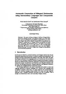
For our purposes, a scientific workflow consists of a number of actors, which are connected via directed edges called channels (Figure 1). An actor is a component (e.g., a web service, shell command, local function, remote job) that can consume and produce data tokens. An actor has zero or more uniquely named ports designated as either input or output. With each port we can associate a structural type (or schema) S describing the structure of data (tokens) flowing through that port. K’s structural type system, inherited from Ptolemy II [7], includes atomic types, e.g., string and double, and complex types such as list and record. In a workflow, actors exchange information using channels that link an output port (token producer) to one or more input ports (token consumers). Workflows are executed according to a model of computation (implemented by a so-called director [7]), which specifies the overall workflow orchestration and scheduling. Here we assume a model of computation that corresponds to a dataflow process network [11]. Figure 1 shows a simple workflow in K for computing species richness and productivity. The workflow performs a number of distinct computations over two input datasets shown on the left of the workflow, which results in the richness and productivity derived data products shown on the right. Semantic Type Propagation. Figure 2 depicts the problem of propagating an input semantic type α through an actor, yielding the output semantic type α0 . A semantic type α associates elements of a schema S with concepts from an ontology O. The goal of
Fig. 1. Simple scientific workflow for computing species richness and productivity [9]
propagation is to automatically generate α0 , given α. This is only possible if something is known about the relation between elements of S and those in S’. A query expression q provides this relation. The query q can approximate2 the actual function f : S → S’ computed by the actor, e.g., q might “overestimate” f such that q(D) ⊇ f (D) for any input data D. The propagation problem is to determine α0 : S’ → O, the semantic type of the output, given the input type α and the query q. We denote this problem as computing α0 = α ◦ q−1 in Figure 2, i.e., the composition of α and (the inverse of) q. Based on our semantic-type framework (Section 3), we describe an initial approach towards solving this problem (Section 4). Our approach places few restrictions on where initial semantic types are given. Semantic types may be provided for input data or for inputs of some actor(s) only, significantly reducing the amount of semantic description required to reuse workflows and actors. A user may also provide additional semantic types at specific points within a workflow, e.g., when the result of a computation creates new data values or adds semantic information. These semantic types are also propagated through actors. The advantages of our approach directly benefit scientific workflow engineers at various stages of workflow construction, including: • Semantic types can be derived at workflow design-time (even before all actors or data are available), and thus can be used as a tool to help workflow engineers build new analyses. For example, propagated types can be presented to the user after two actors are connected, showing the resulting semantic types of combining the steps and the impact on the rest of the workflow. • Scientific workflows can often be executed over different input datasets. The workflow’s global inputs are typically quite generic, while a given dataset may have very specific semantic types. Our approach can propagate these specific semantic types of datasets, resulting in more accurate (specialized) semantic types at data binding-time. • When a workflow is executed, derived data products are automatically given the propagated semantic type, minimizing the effort required to semantically type datasets at workflow runtime. 2
Consider a filter function f that removes outliers and returns only “good” tokens. This function can be modeled as a selection σθ where θ is the filter condition. Obviously, S = S’ in this case, which means that α can be propagated as is (in fact, α0 = α ∧ θ can be derived).
O
O
α
O
α S
workflow step (“actor”)
α′ = α(q-1 ) S
S′ input-to-output semantic type propagation
q
workflow step (“actor”)
S′
q
Fig. 2. Actor with semantic type α, propagated via query q, yielding semantic type α0 .
Another advantage of propagation is ontology augmentation. Consider an actor A2 having as input species richness data. The developer of A2 may provide a semantic type α2 for A2 ’s input, stating that it was designed to “consume” R data.3 Assume a workflow designer has connected the output of another actor A1 to the input of A2 , and for the output of A1 a semantic type α1 has been derived via propagation, indicating that A01 s output is of type sum(O), i.e., the arithmetic sum (resulting from an aggregation) of O data. For the link: α1
α2
A1 −−−−−−→ A2 to be semantically type correct, we must have that α1 is “compatible” with α2 , i.e., sum(O) v R. If we choose to run our propagation system in “automatic mode”, it will augment the given ontology O with this additional axiom. Conversely, the system can be run in “interactive mode”, asking the user to determine whether the inferred axiom is correct and can be included in O, or whether there is something wrong with the connection. This example also illustrates that semantic type constraints between connected actors are “soft” in the sense that one can still execute the corresponding workflow steps, even though doing so may not be semantically meaningful. In contrast, the structural type constraint when connecting A1 and A2 is “hard”, i.e., the schema types S1 and S2 must satisfy a subtyping constraint S1 � S2 for the connection to be executable.
3
The Semantic-Type Framework
Query Expressions. Actors may have an associated query expression q, which may be derived from the component implementation (e.g., from a script or generated data transformation) or explicitly given by a service provider (e.g., for “black-box” actors whose inner workings are unknown). The most general form of a query expression is a logic constraint ϕS∪S’ associating schema elements of the input port(s) S of an actor with those of its output port(s) S’. In analogy to data integration terminology, we can call q an Output-as-View (OAV) mapping if it has the form q = PS’ :- ϕS , and an Inputas-View (IAV) mapping if it has the form q = PS :- ϕS’ . Here, q is a logic atom defining data elements of the output schema S’ (or the input schema S) in terms of the query ϕS (or ϕS’ ) over S (or S’, respectively). In this paper we focus on query expressions 3
We use SC to denote concepts from an ontology O.
given in the OAV form. Query expresssions can contain the standard relational operators select, project, join, union, and group-by with aggregation (i.e., sum, count, avg, min, and max). Note that a query expression q does not need to exactly capture the function f being computed by an actor. It is sufficient if q approximates f such that all structural associations between S and S’ are preserved. These structural associations will then be used to propagate the semantic types from S to S’. We use Datalog notation [1], extended with aggregrate functions and grouping, to denote query expressions. Relations are denoted using capitals (Biom, Sscd, etc.) and variables are in lower-case (x, y, . . . ). For example, query q1 approximates the Create Seasonal Community component of Figure 1: Biom1(o, y, s, t, p, b) :- Biom(o, y, s, t, p, b), Sscd(p)
(q1 )
This query selects Biom tuples (returned as Biom1 tuples) whose p-values are present in the Sscd data set. Biom represents a relational table consisting of measurements (with measurment-id o) of biomass b for a particular species p, year y, season s, and plot t. The Sscd relation contains species found within a particular community. Query expressions can contain group-by with aggregate operators syntactically written agg(x|¯y), where agg is the name of the aggregate operation, x is the aggregation variable, and y¯ is a comma-separated list of grouping variables. We introduce a new variable in the head of an aggregate query and assign it (using the “^” symbol) to the aggregate expression. For example, query q2 gives the annual biomass for each plot and species (the Compute Annual Biomass actor): Biom2(y, t, p, z ^ sum(b|y, t, p)) :- Biom1(o, y, s, t, p, b)
(q2 )
Union operations are expressed in the normal way using multiple rules. For example, query q3 returns annual occurrence measurements (the Compute Occurrence actor): Biom3(y, t, p, 1) :- Biom2(y, t, p, b), b > 0 Biom3(y, t, p, 0) :- Biom2(y, t, p, b), b ≤ 0
(q3 )
Ontologies. We use description logic to express ontologies, which are used to formally define the terms (concepts) in a given domain and their relationships (roles). The OWL-DL standard is also used in K for storing and exchanging ontologies. A simple ontology is shown in Figure 3, representing definitions for ecological measurements (concept O) and ecological concepts such as A, R, etc. According to the underlying description-logic definitions (not shown in the figure), every observation has exactly one observed property (e.g., abundance) and item (e.g., species), and one or more spatial and temporal contexts. We assume a reasoning system is available to compute subsumption hierarchies from concept and role definitions. We use subsumption in particular to determine whether channels defined between actors are semantically compatible. Semantic Types. Each structural type of a dataset, input, or output port, may be given a semantic type, which in its most general form is a logic constraint αS∪O associating
Observation
observedProperty Observable Property is-a
Occurrence
is-a
Productivity
spatialContext
observedItem Observable Item is-a
Richness
is-a
Species
temporalContext
Spatial Entity is-a
Plot
Temporal Entity is-a
Season
is-a
Year
is-a is-a
Abundance is-a
Winter
is-a Spring
is-a Fall
Biomass
Fig. 3. Simplified ecological measurement ontology shown graphically
Biom(o, y, s, t, p, b) Biom(o, y, s, t, p, b) Biom(o, y, s, t, q, b) ∧ s = ‘W’ Biom(o, y, s, t, q, b) ∧ s = ‘S’ Biom(o, y, s, t, q, b) ∧ s = ‘F’ Biom(o, y, s, t, p, b) Biom(o, y, s, t, p, b) Biom(o, y, s, t, p, b)
→ → → → → → → →
O(o) C(o, y) ∧ Y(y) C(o, s) ∧ W(s) C(o, s) ∧ S(s) C(o, s) ∧ F(s) C(o, t) ∧ P(t) I(o, p) ∧ S(p) P(o, b) ∧ B(b)
(1) (2) (3) (4) (5) (6) (7) (8)
Fig. 4. An example semantic type linking biom elements to elements
schema elements S with concept expressions from an ontology O. We consider a syntactic form that we call Terminology-as-View (TAV) in which the ontology structure O is “virtually populated” with elements from the data schema S, thereby establishing the desired semantic type α = αS → αO . More precisely, we consider semantic types having the form α = ∀ x¯∃¯y αS ( x¯) → αO ( x¯, y¯ ), where αS ( x¯) is a query over a data structure S, linking selected elements (captured via bindings of the variables x¯) to concept expressions αO ( x¯, y¯ ) over the ontology O. Figure 4 gives example semantic-type constraints linking schema elements of the Biom data structure S used above to concepts and roles from the ontology O given in Figure 3. Line (1) states that every measurement in Biom represents an O. Line (2) states (i) that all year values in biom are instances of the Y concept, and (ii) that the year instance is a temporal context of the corresponding observation instance. Lines (3–5) are similar, but contain an additional condition on the value of the season, and lines (7–8) annotate species and biomass values.
4
Propagating Semantic Types
We divide our approach for propagating semantic types through actors into three classes of increasing expressibility for query expressions: conjunctive queries (i.e., containing only select, project, and join operations); conjunctive queries with aggregation; and conjunctive queries with aggregation and union. The Conjunctive Case. Let query q and semantic type α be of the form: – q = ∀¯u∃¯v PS’ (¯u) :- ϕS (¯u, v¯ ) – α = ∀ x¯∃¯y αS ( x¯) → αO ( x¯, y¯ ) Here, PS’ is a logic atom over the output schema S’ and ϕS is a query over the input schema(s) S. Similarly, for semantic types α, we relate instances of a schema S with those of an ontology O via subformulas αS and αO , respectively. The basic idea of computing α0 = α ◦ q−1 is as follows. We would like to relate instances of the output schema S’ with instances of O. Assume a substitution that satisfies ϕS (in q) implies αS (in α). For this substitution we can establish the desired relation q−1
α
between S’ and O, denoted abstractly as S’ { S { O. More precisely, we consider q as a logical constraint of the form: q(¯u) = PS’ → Q1 ∧ · · · ∧ Qn ∧ ψ | {z } ϕS
and α of the form α( x¯) = A1 ∧ · · · ∧ Ak → αO | {z } αS
where PS’ is a logic atom over the output schema S’, Qi and A j are logic atoms over the input schema(s) S, and ψ and αO are quantifier-free formulas. We assume that all ∃-quantified variables (¯v and y¯ above) have been eliminated through Skolemization so that q and α can be seen as (implicitly) ∀-quantified formulas with variables u¯ and x¯.4 For propagating α “through” q we use the inverse of q, i.e., the left-to-right (‘head → body’) direction of the query (‘head :- body’). This direction is the one used in LAVstyle query rewritings (e.g., for sound views) and also corresponds to the usually implicit direction in Datalog-style rules (aka Clark’s completion [10]). More precisely, q is defined by the equivalence ∀¯u∃¯v PS’ (¯u) ↔ ϕS (¯u, v¯ ) where intuitively, if ϕS (¯u, v¯ ) is a result of the query q (in a model M), then PS’ (¯u) must also be true (in M) [10,12]. Observe that q can be written as a conjunction q1 ∧· · ·∧qn ∧qψ with qi = PS’ → Qi , and qψ = PS’ → ψ. If we assume there is a substitution σ that unifies some atom Qi0 and some A j0 , i.e., Qσi0 = Aσj0 5 , we can infer from qi0 = PS’ → Qi0 and α a new semantic type α0i0 of the form: α0i0 = PσS’ ∧ (αS \ A j0 )σ → ασO 4 5
We assume that the variables u¯ in q(¯u) are disjoint from the variables x¯ in α( x¯). T σ denotes the result of applying σ to a term T .
where (αS \ A j0 ) is the conjunction A1 ∧ · · · ∧ Ak with A j0 removed. It is easy to show that the semantic type α0i0 is implied by qi and α. In this way, by successively “resolving away” atoms A j from αS with matching atoms Qi from ϕS , we can obtain new semantic types α0 that relate elements of the output schema S’ to those in the ontology O. Example 1 (Propagation for Conjunctive Queries). Consider query q1 expressed as a first-order formula: Biom1(o, y, s, t, q, p, b) → Biom(o, y, s, t, q, p, b) ∧ Sscd(p)
(1)
This formula can be resolved with semantic-type expression (8) in Figure 4, resulting in the new formula: Biom1(o, y, s, t, q, p, b) → P(o, b) ∧ B(b)
(2)
Observe that we now have biomass values b for the output schema Biom1 semantically typed as B instances, linked through the P role. Handling Aggregation. The approach for propagating conjunctive queries can also be used for aggregation, due to the particular syntactic representation used to express aggregate operators. As mentioned in Section 2, we perform an additional step for aggregate queries that connects aggregate operators to certain ontology concept defintions, which can be further used to infer new connections between components. The following simple example demonstrates how propagation is used with aggregation. Example 2 (Propagation for Aggregate Operators). Consider the following Skolemized query q for the Compute Richness actor of Figure 1: Biom4(y, t, r ^ sum(c | y, t)) → Biom3(y, t, f p (y, t, c), c)
(1)
Biom3(y, t, p, c) → O(c)
(2)
and the following (additional) output semantic type of the Compute Occurrence actor6 :
We can resolve (1) and (2) above, resulting in the new formula: Biom4(y, t, r ^ sum(c | y, t)) → O(c)
(3)
Biom4(y, t, r ^ sum(c | y, t)) → sum(O)(r)
(4)
Observe that in this example we have “preserved” the fact that r is the sum of a variable c, and that values for c are O instances. Thus, we can see that r is exactly the sum of O. For propagated semantic types of this form, we also propagate a semantic-type expression where r is an instance of a new concept formed from the aggregate name and c’s assigned concept. Thus, for the previous propagated semantic type we also propagate:
With this additional step it becomes possible, e.g., to determine that the Compute Richness actor can safely be connected to other actors that input R data, leveraging definitions in the ontology such as sum(O) v R. Here, sum(O) represents an ontology concept that is “linked” with a certain functionality in the query expression language. 6
e.g., given by the actor developer to account for the new data produced by Compute Occurrence
Handling Union. Let the union query q be of the form: q = ∀¯u∃¯v PS’ (¯u) :- ϕ1S (¯u, v¯ ) ∀¯u∃¯v PS’ (¯u) :- ϕ2S (¯u, v¯ ) which can also be written as the constraint q(¯u) = PS’ → ϕ1S ∨ ϕ2S for ϕ1S = Q11 ∧ · · · ∧ Q1n ∧ ψ1 and ϕ2S = Q21 ∧ · · · ∧ Q2n ∧ ψ2 . To resolve q and α, we rewrite q into clausal form, generating the two formulas q0 (¯u) = PS’ ∧ ¬ϕ2S → ϕ1S and q00 (¯u) = PS’ ∧ ¬ϕ1S → ϕ2S . Observe that q0 (and similarly q00 ) can be rewritten as a conjunction q01 ∧· · ·∧q0n ∧q0ψ with q0i = PS’ ∧ ¬ϕ2S → Q0i and q0ψ = PS’ ∧ ¬ϕ2S → ψ1 . Assume there is a substitution σ that unifies some atom Qi0 and some A j0 for a semantic type α( x¯) = A1 ∧ · · · ∧ Ak → αO . From q0 and α we can infer α0 of the form: α0 = PσS’ ∧ ¬ϕ2S σ ∧ (αS \ A j0 )σ → ασO where (αS \ A j0 ) is the conjunction A1 ∧ · · · ∧ Ak with A j0 removed, similar to the regular conjunctive case. As before, we successively “resolve away” atoms A j from αS with matching atoms Q1i from ϕ1S . We note that α0 may not be in the desired form for semantic types (it may not be in clausal form) because, e.g., ¬ϕ2S may result in a disjunctive formula. For such cases, we can apply the following simple conversion. Assuming query expressions q = P → (Q ∧ R) ∨ (Q0 ∧ R0 ) and semantic types α = Q → αO , using resolution we infer, e.g., α0 = P∧¬(Q0 ∧R0 ) → αO , which becomes α01 = P∧¬Q0 → αO and α02 = P∧¬R0 → αO . Example 3 (Propagation for Union). Consider query q3 as the first-order formula: Biom3(y, t, p, c) → (Biom2(y, t, p, fb (y, t, p)) ∧ fb (y, t, p) > 0 ∧ c = 0) ∨ (Biom2(y, t, p, fb (y, t, p)) ∧ fb (y, t, p) ≤ 0 ∧ c = 1)
(1)
and the Skolemized semantic-type propagated from the Compute Annual Biomass actor (note that we only include the result z of the original aggregrate operator): Biom2(y, t, p, z) → I( fo (y, t, p), p) ∧ S(p)
(2)
Rewriting (1) into clausal form gives: Biom3(y, t, p, c) ∧ ¬(Biom2(y, t, p, fb (y, t, p)) ∧ fb (y, t, p) > 0 ∧ c = 0) → Biom2(y, t, p, fb (y, t, p)) ∧ fb (y, t, p) ≤ 0 ∧ c = 1
(3)
Biom3(y, t, p, c) ∧ ¬(Biom2(y, t, p, fb (y, t, p)) ∧ fb (y, t, p) ≤ 0 ∧ c = 1) → Biom2(y, t, p, fb (y, t, p)) ∧ fb (y, t, p) > 0 ∧ c = 0
(4)
Resolving (2) and (3), e.g., results in the new annotation: Biom3(y, t, p, c) ∧ ¬(Biom2(y, t, p, fb (y, t, p)) ∧ fb (y, t, p) ≤ 0 ∧ c = 1) → I( fo (y, t, p), p) ∧ S(p) We can now rewrite (5) into our desired form for semantic types.
(4)
5
Concluding Remarks
The creation of rich semantic-type annotations can be a complex task, making the problem of automatic generation of such types important for scalable “metadata-intensive” and “semantics-intensive” scientific applications. To this end, we have developed and presented a semantic-type propagation approach and sketched how queries involving selection, projection, join, aggregation, and union could be handled. Our approach is based on an inference procedure similar to the chase [1], which itself can be seen as a form of resolution [4]. Propagating semantic types is also related to work on data provenance [3,8] where the focus (in terms of propagation) is on supporting simple textbased annotations of relational table cells (instead of formulas over schemas), and on augmenting SQL to allow users to state specific schemes for propagating these valuebased annotations to query results. In contrast, our semantic types are formal logicbased descriptions linking structural types to ontologies. These semantic types can be propagated within the framework of scientific workflows. We are currently investigating the properties of a specialized inference procedure, based on algorithms in [15] for composing mappings given by logic constraints. We plan to implement semantic type propagation within K as part of future work.
References 1. S. Abiteboul, R. Hull, and V. Vianu. Foundations of Databases. Addison Wesley, 1995. 2. C. Berkley, S. Bowers, M. Jones, B. Ludaescher, M. Schildhauer, and J. Tao. Incorporating semantics in scientific workflow authoring. In Proc. of SSDBM, 2005. 3. D. Bhagwat, L. Chiticariu, W. C. Tan, and G. Vijayvargiya. An annotation management system for relational databases. In Proc. of VLDB, 2004. 4. J. Biskup and A. Kluck. A new approach to inferences of semantic constraints. In In Proc. of Advances in Databases and Information Systems, 1997. 5. S. Bowers and B. Lud¨ascher. An ontology-driven framework for data transformation in scientific workflows. In Proc. of DILS, volume 2994 of LNCS, 2004. 6. S. Bowers and B. Lud¨ascher. Actor-oriented design of scientific workflows. In 24th Intl. Conf. on Conceptual Modeling (ER), 2005. 7. C. Brooks, E. A. Lee, X. Liu, S. Neuendorffer, Y. Zhao, and H. Zheng. The Ptolemy II Manual (vol. 1-3). Technical report, UC Berkeley, 2004. 8. P. Buneman, S. Khanna, and W. C. Tan. Why and where: A characterization of data provenance. In Proc. of ICDT, volume 1973 of LNCS, 2001. 9. D. Chalcraft, J. Williams, M. Smith, and M. Willig. Scale dependence in the speciesrichness-productivity relationship: The role of species turnover. Ecology, 85(10), 2004. 10. K. L. Clark. Negation as failure. In Logic and Databases. Plemum Press, 1977. 11. E. A. Lee and T. M. Parks. Dataflow process networks. Proc. of the IEEE, 83(5), 1995. 12. M. Lenzerini. Data integration: A theoretical perspective. In Proc. of PODS, 2002. 13. B. Lud¨ascher, I. Altintas, C. Berkley, D. Higgins, E. Jaeger, M. Jones, E. A. Lee, J. Tao, and Y. Zhao. Scientific workflow management and the kepler system. Concurrency and Computation: Practice & Experience, 2005. to appear. 14. B. Lud¨ascher, A. Gupta, and M. E. Martone. Model-based mediation with domain maps. In Proc. of ICDE, 2001. 15. A. Nash, P. A. Bernstein, and S. Melnik. Composition of mappings given by embedded dependencies. In Proc. of PODS, 2005.