P. Cignoni, G. Impoco, I. Miraglia, R. Scopigno. Istituto di Scienza e Tecnologie ..... References. [1] 3DScanners. The ModelMaker scanning systems. More info ...
Towards Automatic Registration Of Range Maps P. Cignoni, G. Impoco, I. Miraglia, R. Scopigno Istituto di Scienza e Tecnologie dell’Informazione (ISTI) Consiglio Nazionale delle Ricerche Via Moruzzi 1, 56125 Pisa, ITALY. Email: {cignoni | impoco | scopigno }@isti.cnr.it
Abstract The range map registration (or alignment) phase is the main bottleneck in the 3D scanning pipeline due to the amount of user intervention required. The standard approach to registration consists of an initial rough alignment followed by an automatic refining technique (ICP). Automatic registration is an active research area, since it is the missing component to fully automatise the scanning process. Although many efforts have been made in order to avoid the manual placement, none of the existing technologies seems to be adequately accurate and flexible. This paper addresses the problem of providing a good initial guess to the ICP algorithm, by tracking the 3D-scanner motion using well known (and low cost) computer vision techniques. The proposed technique is shown to be effective and to generate sufficiently accurate guesses in the majority of the possible configurations.
1
Introduction
3D scanning technologies evolved considerably in the last few years, both on the side of hardware devices [5] and software tools for post-processing raw scanned data [2]. Complex 3D objects cannot be acquired in a single shot. Hence, multiple range scans must be acquired in order to cover the whole object’s surface (hundreds in the case of medium or large complexity artifacts). Then, in a postprocessing phase, these individual scans have to be seamlessly integrated in a unique 3D model. Since the range maps provided by most 3D range scanners are defined in a coordinate system which depends on the relative position of the scanner and the object, they must be registered (or aligned) into a common coordinate system. The standard approach to registration subdivides the task in an initial pairVMV 2003
wise alignment (each range map is aligned with all of the partially overlapping ones) and a final global alignment [21]. The pairwise phase consists of an initial rough alignment, usually performed in an interactive manner by the user, followed by an automatic refining technique, the Iterative Closest Point (ICP) method [4, 8, 28]. The initial placement is in general assisted by an operator, and it is the main bottleneck of the entire process due to the overall time consumed and the skills required. Although many efforts have been made in order to avoid the manual placement, none of the existing technologies seems to be adequately accurate and flexible. This paper addresses the problem of finding automatically a good initial guess for the ICP algorithm, in order to fully automatise the registration process. Many different methods have been adopted in practical situations but none of them seems to be sufficiently flexible to be considered as a general solution. Those approaches can be divided in two main classes: automatic (software-based) methods which recover the required roto-translation transformation form the analysis of matching features present in consecutive adjacent overlapping range maps; and methods which track the relative position of the scanner and the object acquired. The first type of approaches [17] are theoretically stimulating, but the available solutions do not guarantee sufficient robustness since we have to search for corresponding features on unknown subregions of overlap, and there exist many situations in which the symmetry or the lack of significant geometric features of the acquired object does not allow a correct alignment. The second approach can be implemented by tracking either the scanner or the object. Some high-end systems make use of calibrated positioning of the scanner; the scanner pose can be tracked by a coordinate measurement machine, a 6-DOF Munich, Germany, November 19–21, 2003
2.1
robotic arm or any other type of computer controlled gantry [18, 1]. Good results obtained with this approach are balanced by high costs and lack of flexibility (cheap systems support a very small scanning volume, high-end systems are heavy and complex to install). A less expensive solution is to adopt acoustic, magnetic [20], inertial [15], or optical tracking subsystems. While the first two approaches do require controlled environments for avoiding producing noisy data and the third suffers from accumulation of estimation errors (drift) [27], optical systems seem more promising for our application. Finally, an alternative tracking solution can be to maintain the scanner in a fixed position and to move the object in a computer-controlled manner (for example, by means of a calibrated turntable [11]). This approach is sufficiently cheap, but it imposes some restrictions on the dimension and weight of the objects which can be treated. Therefore, we decided to investigate the use of optical tracking techniques because of their low cost and greater flexibility. Our idea was to reconstruct the rigid motion undergone by the 3D-scanner using a sequence of intensity images captured by means of low-cost digital cameras moving jointly with the scanner. This is a well known problem in Computer Vision, thus some background information and knowledge can be reused in this peculiar problem. Our goal is to get rid of the human intervention needed for the initial rough alignment in order to automatise all the post-processing scanning process. The paper is structured as follows. Section 2 is a short overview of the techniques used to automatise the alignment phase. Section 3 introduces the motion tracking problem, and Section 4 describes our alignment system and the tracking techniques employed. Some experimental results are shown in Section 5. A brief discussion closes the paper.
Automatic Approaches
A first approach is to design a purely software method to automatically reconstruct the initial rototranslation from just some processing of the available geometrical information [17]. It is very hard to produce sufficiently robust results in a completely automatic manner, especially when we cannot assume a high degree of coherence (i.e. a small overlap region) between successive range maps. One of the best results in this field has been attained in [24]. The proposed system assumes that a small object is slowly moved in front of a very fast acquisition device that is able to acquire about 60 range maps per second. In this way the authors can rely on a strong coherence among two consecutive range maps and therefore on the correct working of the ICP algorithm for their alignment. The main drawbacks of this approach are: the limitation on the size of scannable objects that must be moved in front of the (fixed) scanner; and the very large number of range maps acquired (the higher the frame rate, the higher the coherence, but also more complex and redundant the set of scanned samples). Furthermore, the possible failure of the ICP algorithm, due to many different reasons like too fast motion in front of the scanner or flat sliding areas of the object, are not discussed. Interesting results can be obtained when 2D intensity maps are acquired together with the range map [23]. Using computer vision techniques, automatic registration is performed between the intensity images corresponding to successive scans. Range maps are then aligned making use of this registration. This algorithm is shown to be able to align range data automatically in many cases, or at least provide a good initial guess for the ICP algorithm. However, again this solution assumes substantial coherence between the acquired range maps and requires large overlapping regions (more than 2030%). Moreover, 2D matching algorithms are sufficiently accurate only if the viewpoints of the two intensity images are close together. Low time efficiency is another critical issue of these techniques.
2 Related Work Automatic registration is an active research area. The problem has been addressed from many different viewpoints. The different approaches can be classified in automatic (software-based) methods, and methods which make use of mechanical tracking systems, or non-contact tracking systems. In the following all the three schemes are introduced.
An image-based approach has been proposed also in [3], with the slightly different objective to improve the accuracy of the ICP process when the shape features of range data are not sufficient to drive the geometry-based ICP optimisation. 666
2.2
Mechanical Tracking
ject to climatic variation and do not work correctly with high temperature or humidity. Furthermore, unlike magnetic waves, acoustic ones cannot go through obstacles and can suffer from acoustic reflections if surrounded by acoustically reflective surfaces. Again, working in non-controlled environments may become a problem. Optical tracking systems work by matching high contrast features between successive frames in a video sequence [12, 10]. Typical features employed are corners, edges, and lines or gray-level pixel patches. Tracked features can be part of the natural scene or fiducial markers attached to the object or to the scanning area. Optical trackers can be totally passive or make use of light emitters as fiducial markers. Data can be acquired by means of low-cost consumer electronics, e.g. digital low-cost cameras. Feature matching algorithms can be computationally expensive as they extract features or statistical information directly from raster images. Despite of this, optical approaches can be faster and more accurate than both acoustic and magnetic ones [22]. Accuracy can be further improved using prediction-correction schemes. Like acoustic techniques, the major drawback of optical systems is the requirement that an unobstructed line-of-sight between the tracked elements and the camera must be maintained all over the tracking-time (but redundancy of the tracked elements makes this drawback less significant). For a more detailed comparison of tracking techniques see [22, 27].
Mechanical tracking systems can produce either a rough or precise estimate of the roto-translation between successive scans [18, 1]. The scanner can be attached to a coordinate measurement machine which keeps track of its position with a high degree of accuracy. Mechanical arms, both active and passive, have been also successfully used. Nevertheless, these techniques are not widely used because of the high cost and encumbrance in narrow environments. In less expensive systems an initial registration can be easily computed by positioning the object to be scanned on a turntable. Knowing the degree of rotation of the turntable an estimate of the motion between consecutive scans can be easily obtained [11]. The problem of this approach is that the object to be scanned must fit on the turntable and the system provides only a cylindrical set of scans which is in general not sufficient to reconstruct in an accurate manner self-occluding objects.
2.3
Non-mechanical Tracking
Non-mechanical approaches try to track the scanner position over time using inertial, magnetic, acoustic, or optical technologies. Inertial sensing is based on gravity forces. Inertial trackers make use of gyroscopes and accelerometers to measure linear and angular acceleration relative to a fixed reference system. Position orientation, can be computed by integration. Magnetic tracking systems (see for example [20]) are based on the transmission and reception of electromagnetic signals. Magnetic trackers do not suffer from line-of-sight obstruction issues as electromagnetic fields can travel through minor obstructions, and they require a little computation to obtain an estimate of the object motion. However, electronic devices and conductive or ferrous metals usually distort the projected electromagnetic field, leading to highly inaccurate estimates. As a consequence they need a controlled environment and ipso facto they lack of flexibility, since in many applications the acquisitions cannot be done in a lab (e.g. cultural heritage and industrial quality control). Acoustic techniques use ultrasonic emitters to determine the location of the tracked object (using a sort of time-of-flight computation). As acoustic waves travel through air, these systems are sub-
3 Motion Estimation In order to choose the tracking technology that best fits our problem, a brief requirements analysis is needed. We want to build a low-cost system that can be used during the acquisition of objects of arbitrary size and in different environments (mainly, in non-controlled environments, such as for example a museum). Hence, we should avoid mechanic tracking systems because of high costs, complex installation and little flexibility. Methods based on the adoption of a turntable are also not optimal because they support constrained motion and limit the objects’ size and weight. On the other hand, geometric methods generally assume high coherence between successive scans. Tracking scanner position using features of the surrounding environment is an approach that do not 666
roto-translation undergone by the scanner (S in figure) since the last range map acquisition. At the successive scan, the motion estimate is sent to the computational unit which runs the ICP algorithm to align the last acquired range map to the previous ones. The motion estimate will be used in place of the standard initial manual placement. If the estimate is sufficiently accurate, the ICP algorithm returns the correct alignment. An important point
rely on the shape of the object to be scanned. Consequently we have to orient ourselves to nonmechanical motion tracking approaches. Among these, we discard magnetic as well as acoustic techniques because of their need for controlled environments and low accuracy, and inertial ones because of low tracking autonomy (due to accumulation of errors). Optical technologies seem therefore the best choice because of their higher flexibility and low-cost.
3.1
An Optical Tracking System
Among optical techniques, one of the most studied is camera tracking. It is a well known problem in the field of computer vision research, with a rich literature [12]. A standard system setup is defined in [9, 6]. The basic steps of a general tracking algorithm are as follows: 1. Images of the real world are taken by the camera and features are extracted. 2. Using the extracted features, the tracking unit estimates camera motion. Motion estimation is based on a prediction-correction scheme. 3. Feature positions are updated using the current estimate and bad features are rejected. 4. The remaining (good) features are used as input to the system together with features extracted from new frames, in order to compute a new motion estimate.
3.2
Figure 1:
Architecture of the proposed optical tracking system.
with respect to the accuracy of the tracking system is that we are able to give some feedback to the tracking algorithm. In fact, after the last range map has been registered with the previous one, the relative position and orientation of the two scans is known in a precise manner, due to the result of the execution of ICP. It is therefore possible to correct the current approximate motion estimate given by the tracking unit using the output of the ICP algorithm, thus avoiding the accumulation of estimation errors as the scanning process goes on.
Architecture of our tracking system
4 Camera Pose Estimation
Our system consists of a number of digital cameras mounted rigidly on the 3D-scanner, and a computational unit running both the motion tracking software and the ICP algorithm. In the current set-up, we use two calibrated cameras in order to be able to recover the exact motion of the scanner. Using a single camera it is possible to estimate the exact rotation, but the translation can be computed up to a scale factor. Instead, employing a calibrated stereo rig the scale factor can be calculated, and this allows to compute (by triangulation) the 3D position of points generating corresponding features. Figure 1 gives a graphic description of the whole scanning system. Cameras, shown as C1 and C2, capture a video sequence of the environment and transmit all data to the tracking unit. The motion tracker continuously updates its estimate of the
In this section the tracking engine employed will be explained in detail. Each algorithm has been chosen for its peculiarities which make it more suitable with respect to the requirements of our application. In the following, firstly the standard framework will be introduced then our particular choices will be discussed.
4.1
Standard Camera Pose Estimation
A typical image-based tracker is composed by a number of different modules: • feature detector, which extracts relevant features directly from raster images (usually graylevel); 666
• feature matcher, used to match corresponding features detected in two consecutive perspective images; • motion tracker, which estimates the motion undergone by the camera, given a set of corresponding features in two consecutive frames (or in a a stereo pair); • prediction-correction (usually Kalman filter), which enforces coherence in the motion undergone by the camera in a video sequence, by “smoothing down” incoherent estimations. The features most widely used for motion tracking estimation are corners because of their robustness with respect to variations in lighting conditions of the scene, and invariance under translation, rotation and scale change [26]. In our implementation of the tracking engine we have used the wellknown Harris corner detector [13], which is shown to be the most robust with respect to rotation and scale change in the scene [25]. Corners are searched in the gradient of the smoothed image, then corner pixel coordinates are converted into subpixel coordinates by averaging pixel intensities in a neighbourhood of the corner. For the matching of corresponding features, we have used the feature tracker proposed by Lucas and Kanade [19], which is an iterative tracking algorithm based on matching of graylevel patches. Good features are located by examining the minimum eigenvalues of 2 by 2 gradient matrices defined for each image pixel. In order to be able to match distant features while keeping low the computational burden on the system, we have used a pyramidal multiresolution implementation. The Lucas-Kanade algorithm is executed over a pair of coarsely sub-sampled images, then the match is refined on the immediately finer level in the hierarchy, and so on recursively. At the finest level of the pyramid, a set of candidate matches is found (see Figure 2).
Camera motion is computed using the Least Median of Squares (LMedS) algorithm [29]. LMedS exploits the epipolar constraint [12] in order to establish a robust set of correspondences between two perspective images. The candidate matches are validated (disambiguated) using a relaxation technique which takes into account the contribution of neighbouring candidate matches, in order to compute the strength of a match. Candidate matches whose strength falls below a fixed threshold are discarded. The retained matches are used to compute the effective roto-translation. After the camera motion has been estimated by the tracking unit, inter-frame coherence is enforced by means of a prediction-correction scheme introduced by Kalman [16]. A prediction of the new position is done based on the previous estimates. Then, as soon as new measurements are available, new features are integrated in the system and a new motion estimate is transmitted. An advantage of this technique is that one can tune the degree of confidence in the measurement accuracy by weighting new measurements against previous estimates. As a consequence, outliers (i.e. bad features) can be detected and discarded.
4.2
An Ad-Hoc Approach
As an alternative to the LMedS solution [29], we have also adopted a simpler approach to estimate camera motion from image correspondences. Using a calibrated stereo rig, it is possible to estimate the spatial coordinates of the points corresponding to matched features. An example of stereo rig is shown in Figure 3. Here mi and m�i are two corre-
A stereo rig. The point Mi is projected onto the image planes π and π � , generating the match (mi , m�i ).
Figure 3:
sponding features, and Mi is the point whose projection on the image planes π and π � are mi and m�i respectively. The set of points Mi corresponding to the matches (mi , m�i ) is a sort of coarse geometric
Figure 2:
Corner matches in two consecutive images after the cross-validation step (see Section 4.2).
666
second image to features in the first one. Let Bd (x) be the ball of radius d centred at x. For each corner c1 in the first image, we check if the corresponding pixel c2 = F12 (c1 ) in the second image is such that ∃c�2 : c2 ∈ Bh� (c�2 ), where c�2 is a corner in the second image and h� is a distance threshold. Let c�1 = F21 (c�2 ). Then the couple (c1 , c�2 ) is retained if c�1 ∈ Bh (c1 ), with h a threshold possibly distinct from h� . Considerable improvements in motion estimation accuracy were obtained enabling cross-validation, while the computational overhead is negligible. On the other hand, since we discard many candidate matches, if the scene does not contain a sufficient number of features the number of good matches could be insufficient to obtain a reliable estimate. An example of cross-validation output is shown in Figure 2.
representation of what the two cameras “see”. Assuming fixed the position of these points, camera motion can be recovered computing their relative position with respect to the two camera reference frames. To find the rigid transformation that minimises the least-squared distance between the point pairs we use the direct method described in [14] and [4]. We weighted each point Mi with respect to the accuracy of its position, reconstructed from its projections mi and m�i onto the image planes (see Figure 3). In our experiments we have tested both tracking algorithms. In our preliminary tests we have found that the minimisation procedure on the stereo pair is more reliable and gives more accurate results than the estimation of epipolar geometry. Moreover, from the practical point of view, the minimisation procedure is easier to implement and runs faster than LMedS. For the these reasons, we have used the minimisation procedure in our experimental testbed. The main drawback of this simple solution is its sensitivity to potential false matches and to errors in the computation of the point locations. In order to improve the robustness of the minimisation procedure, we have designed a simple cross-validation scheme to discard a great number of false matches before the tracking algorithm is run. It relies on the observation that if a point in the first image matches a point in the second image, than the inverse must be true, i.e. the point in the second image must match the corresponding point in the first image. This concept is illustrated in Figure 4. Let us define F12 as
5 Experimental Results This paper reports just the first results of our ongoing project, obtained by testing our approach on a synthetic testbed. We decided to run the first assessment phase on a synthetic environment (the images and range maps are not acquired with a real camera/scanner pair, but rendered from a 3D model) to be able to measure the difference between the actual virtual camera location and the reconstructed one. Since the accuracy of motion estimation does not depend on the extent of the overlapping area between scans, the scanning viewpoints can be chosen in order to fit well with the requirements of the ICP algorithm. Some results are shown for three scenes in Table 1. Results are shown together with the erscene satyr dragon buddha
ICP results aligned average (%) error 40 55 73
44.1 19.2 20.1
(average) error wrt exact RT translation rotation (module) x y z 115.0 129.3 216.3
1.09 1.51 1.20
1.07 1.10 2.26
1.46 1.75 2.58
Table 1:
Some results. Average and translation errors are expressed in millimetres. Rotation error is reported in degrees.
Figure 4: Cross-Validation procedure. The corner c1 is retained
ror between the estimated roto-translation and the ground truth. The second and third column show respectively the percentage of automatically aligned range scan pairs, and the average of the errors computed at the first iteration of the ICP algorithm for each alignment pair; this number denotes the 50percentile of the Hausdorff distance distribution be-
if and only if there exists a point c�2 at distance h� from c2 , such that the distance between the corresponding match, c�1 , and c1 is lower than h.
the function that maps each corner in the first image to a corresponding feature in the second image, and F21 an analogous function from the set of corners in 666
be designed following a range map clustering approach. Namely, when the operator moves the scanner away (e.g. to scan the opposite side of a statue) there will be an abrupt change in scanner pose. Distinct scan clusters will be generated in correspondence of each abrupt position change. Overlapping consecutive scans can be registered on-line during the scanning session, as usual. Non-overlapping consecutive scans cannot be immediately aligned, but they will be registered with respect to different clusters. In a successive alignment phase, overlapping clusters can be registered all together. If the whole object’s surface has been sampled then all the scans can be aligned in few clustering iterations. The alignment library we have implemented, MeshAlign v.2, does support this clustering methodology. Using an auxiliary space-decomposition data structure, MeshAlign automatically adds a new range map to the corresponding cluster and creates all the required pair-wise alignment between this new range map and all the partially overlapping range maps contained in the working set [7].
tween input meshes (i.e. 50% of the mesh surface has a distance larger than that value). The next column shows the error in translation vector (in millimetres), computed as the module of the distance vector between the true and estimated translation. Finally, the last columns show the error with respect to each rotation axis (in degrees), which is simply the module of the difference between estimated and exact angle. Note that in our current implementation we are not taking advantage of Kalman filter. The algorithm fails mainly in scenes where few interest points can be extracted, or under abrupt changes of position/orientation between scans due to accumulation of estimation errors between successive frames. Introducing Kalman filtering should help to cope with those cases. Another critical issue is the choice of framerate. High framerates make easier the task of finding good matches between consecutive frames due to small displacement between corresponding points. On the other hand, since matched points have a short disparity, large numerical errors occur in the computation of 3D points. Conversely, the computation of rototranslation is less error-prone in low framerates, but it is not always possible to establish good matches. As a tradeoff we adaptively insert new frames only when needed for corner matching. Doing this way we can find good matches and, at the same time, assure a large disparity. An example of scan alignment guesses obtained with our algorithm is given in Figure 5.
Figure 5:
6 Concluding Remarks We have presented an effective technique to register automatically a set of partially overlapping range images acquired by a 3D scanner. Experimental results show that the proposed approach is able to automatically align consecutive scans in most cases. On the other hand, since the accuracy of motion estimation does not rely on the results of the ICP algorithm, when automatic alignment fails a good guess on the position of the scan can be given to a human operator. We are planning to further investigate camera tracking techniques in order to obtain more accurate estimates which, in turn, should lead to a higher percentage of automatical aligned scans. Moreover, an extensive experimentation in the framework of a real scanning action in a non-controlled environment (a museum) will be carried on. Finally, we would also like to take a closer look at the relationship between the error measure expressed in Table 1 and the degree of success of the ICP algorithm, in order to assess an a-priori criterion of “alignability” of range maps. Acknowledgements This research was supported by the projects EU IST-2001-32641 “ViHAP3D” and FIRB - “MACROGeo”.
Two alignment guesses, respectively a bad guess and
a good one.
Note that, since the relative roto-translation between scans can be estimated independently with respect to the actual scans, we do not require any overlapping between consecutive range maps. This allows the operator to easily change the acquisition viewpoint, while retaining an estimation of the scanner motion during all the scanning session. This leads to an alignment procedure which could 666
References
[17] G. M. Cortelazzo L. Lucchese. A noise-robust frequency domain technique for estimating planar rototranslations. IEEE Trans. on Signal Processing, 48(6):1769–1786, 2000.
[1] 3DScanners. The ModelMaker scanning systems. More info on: http://www.3dscanners.com/, 2003. [2] F. Bernardini and H. E. Rushmeier. 3D Model Acquisition. In Eurographics 2000, State of the Art Reports Proceedings, pages 41–62. Eurographics Association, August 24–25 2000. [3] F. Bernardini and H. E. Rushmeier. Strategies for registering range images from unknown camera positions. In B.D. Corner and J.H. Nurre, editors, Proc. Conf. on Three-Dimensional Image Capture and Applications II, pages 200–206, Bellingham, Washington, January 24–25 2000. SPIE. [4] P. J. Besl and N. D. McKay. A method for registration of 3-D shapes. IEEE Transactions on Pattern Analysis and machine Intelligence, 14(2):239–258, Feb. 1992. [5] F. Blais. A review of 20 years of range sensor development. In Videometrics VII, Proceedings of SPIEIS&T Electronic Imaging, SPIE Vol. 5013, pages 62– 76, 2003. [6] Jiang Bolan, You Suya, and Neumann Ulrich. Camera tracking for augmented reality media. In IEEE International Conference on Multimedia and Expo (III) 2000, pages 1637–1640, 2000. [7] M. Callieri, P. Cignoni, P. Pingi, and R. Scopigno. MeshAlign v.2 - User Manual. Visual Computing Lab, CNR-ISTI, Pisa (ITALY), 2003. [8] Y. Chen and G. Medioni. Object modelling by registration of multiple range images. International Journal of Image and Vision Computing, 10(3):145–155, April 1992. [9] A. Davison. Mobile Robot Navigation using Active Vision. PhD thesis, Department of Engineering Science, University of Oxford, 1999. [10] E. E. Trucco and A. Verri. Introductory Techniques for 3-D Computer Vision. Prentice–Hall, 1998. [11] A. Fasano, M. Callieri, P. Cignoni, and R. Scopigno. Exploiting mirrors for laser stripe 3d scanning. In 3DIM’03: Fourth Int. Conf. on 3D Digital Imaging and Modelling, page (in press). IEEE Comp. Soc., Oct. 4-8 2003. [12] O.D. Faugeras. Three-Dimensional Computer Vision: A Geometric Viewpoint. MIT Press, 1993. [13] C. Harris and M.J. Stephens. A combined corner and edge detector. In Alvey88, pages 147–152, 1988. [14] B.K.P. Horn. Closed form solutions of absolute orientation using unit quaternions. JOSA-A, 4(4):629– 642, April 1987. [15] Intersense. InertiaCubeTM . More info on: http://www.isense.com/. [16] Rudolph Emil Kalman. A new approach to linear filtering and prediction problems. Transactions of the ASME–Journal of Basic Engineering, 82(Series D):35–45, 1960.
[18] M. Levoy, K. Pulli, B. Curless, S. Rusinkiewicz, D. Koller, L. Pereira, M. Ginzton, S. Anderson, J. Davis, J. Ginsberg, J. Shade, and D. Fulk. The Digital Michelangelo Project: 3D scanning of large statues. In SIGGRAPH 2000, Computer Graphics Proceedings, Annual Conference Series, pages 131– 144. Addison Wesley, July 24-28 2000. [19] B.D. Lucas and T. Kanade. An iterative image registration technique with an application to stereo vision. In Proc. of the 7th IJCAI, pages 674–679, Vancouver, Canada, 1981. [20] Polhemus. scanning system.
The
FastSCAN Cobra More info on: http://www.polhemus.com/fastscan.htm, 2003.
[21] K. Pulli. Multiview registration for large datasets. In Proc 2nd Int.l Conf. on 3D Digital Imaging and Modeling, pages 160–168. IEEE, 1999. [22] R.N. Rohling, P. Munger, J.M. Hollerbach, and T. Peters. Comparison of relative accuracy between a mechanical and an optical position tracker for image-guided neurosurgery. Journal of Image Guided Surgery, J.P. Wiley and Sons Inc., New York, NY, 1(1), 1995. [23] G. Roth. Registering two overlapping range images. In Second International Conference on Recent Advances in 3D Imaging and Modelling, Ottawa, Canada, pages 191–200, October 1999. [24] Szymon Rusinkiewicz, Olaf Hall-Holt, and Marc Levoy. Real-time 3d model acquisition. In Proceedings of the 29th annual conference on Computer graphics and interactive techniques, pages 438–446. ACM Press, 2002. [25] Cordelia Schmid, Roger Mohr, and Christian Bauckhage. Evaluation of interest point detectors. International Journal of Computer Vision, 37(2):151–172, 2000. [26] C.H. Teh and R.T. Chin. On the detection of dominant points on digital curves. T-PAMI, 11:859–872, 1989. [27] G. Welch and E. Foxlin. Motion tracking: No silver bullet, but a respectable arsenal. IEEE Computer Graphics & Applications, 22(6):24–38, November 2002. [28] Z. Zhang. Iterative point matching for registration of free-form curves and surfaces. International Journal of Computer Vision, 13:119–152, 1994. [29] Z. Zhang, R. Deriche, O.D. Faugeras, and Q.T. Luong. A robust technique for matching two uncalibrated images through the recovery of the unknown epipolar geometry. Artificial Intelligence, 78(1-2):87–119, 1995.
666