Towards Bounded-Rationality in Multi-Agent Systems - CiteSeerX

Towards Bounded-Rationality in Multi-Agent Systems: A Reinforcement-Learning Based Approach Anita Raja and Victor Lesser August 23, 2001 Abstract

Sophisticated agents operating in open environments must make complex real-time control decisions on scheduling and coordination of domain activities. These decisions are made in the context of limited resources and uncertainty about outcomes of activities. Many efficient architectures and algorithms that support these control activities have been developed and studied. However, none of these architectures explicitly reason about the consumption of time and other resources by control activities, which may degrade an agent’s performance. The question of how to sequence domain and control activities without consuming too many resources in the process, is the meta-level control problem for a resource-bounded rational agent. The focus of this research is to provide effective allocation of computation and improved performance of individual agents in a cooperative multi-agent system. This is done by approximating the ideal solution to meta-level decisions made by these agents using reinforcement learning methods. Our approach is to design and build a meta-level control framework with bounded computational overhead. This framework will support decisions on when to accept, delay or reject a new task, when it is appropriate to negotiate with another agent, whether to renegotiate when a negotiation task fails and how much effort to put into scheduling when reasoning about a new task. The major contributions of this work will be: a resource-bounded framework that supports detailed reasoning about scheduling and coordination costs; a scheduling paradigm that can support parameters to control scheduling effort, horizon and slack; and a simulation environment for testing and comparing the performance of agents.

1

Contents 1 Introduction 1.1 Assumptions . . . . . . . . . . . 1.2 Agent Decision Space . . . . . . . 1.3 Proposed Agent Architecture . . . 1.4 Taxonomy of meta-level decisions

. . . .

. . . .

. . . .

. . . .

. . . .

. . . .

. . . .

. . . .

. . . .

. . . .

. . . .

. . . .

. . . .

. . . .

. . . .

. . . .

. . . .

. . . .

. . . .

. . . .

. . . .

. . . .

. . . .

. . . .

. . . .

. . . .

3 4 5 5 7

2 Solution Approach 11 2.1 Description of State features . . . . . . . . . . . . . . . . . . . . . . . . . . . . . 13 2.2 Exogenous Events and Related Actions . . . . . . . . . . . . . . . . . . . . . . . 16 2.3 An example . . . . . . . . . . . . . . . . . . . . . . . . . . . . . . . . . . . . . . 23 3 Anticipated Contributions

30

4 State of the Art in Meta-level Control Research 31 4.1 Bounded Rationality and Meta-Level Control . . . . . . . . . . . . . . . . . . . . 31 4.2 Multi-agent Reinforcement Learning . . . . . . . . . . . . . . . . . . . . . . . . . 33 5 Work Plan and Evaluation

33

A Background Information 36 A.1 Markov Decision Processes . . . . . . . . . . . . . . . . . . . . . . . . . . . . . . 36 A.2 The TÆMS Modeling Language . . . . . . . . . . . . . . . . . . . . . . . . . . . 36 B Chapters in the Dissertation

38

C Abstract Formalization of the Problem

38

D Detailed Markov Decision Process

46

2

AGENT

Sensors

Problem Solver

ENVIRONMENT

Effectors

Scheduling Component

Coordination Component

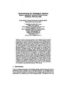
Figure 1: Classical architecture of a bounded rational agent

1 Introduction Open environments are dynamic and uncertain. Sophisticated agents operating in these environments must reason about their local problem solving activities, interact with other agents, plan a course of action and carry it out. All these have to be done in the face of limited resources and uncertainty about action outcomes and the actions of other agents in real-time. Furthermore, new tasks can be generated by existing or new agents at any time, thus an agent’s deliberation must be interleaved with execution. The planning, scheduling and coordination of tasks are non-trivial, requiring either exponential work, or in practice, a sophisticated scheme that controls the complexity. Agent activities can be broadly classified into three categories - domain,control, and meta-level control activities. Domain activities are executable primitive actions which achieve the various high-level tasks. Control activities are of two types, scheduling activities which choose the high level goals, set constraints on how to achieve them and sequence the domain level activities; and coordination activities which facilitate cooperation with other agents in order to achieve the high-level goals. Agents perform these control activities to improve their performance. Many efficient architectures and algorithms that support these activities have been developed and studied[24, 4, 27]. Figure 1 describes the classic agent architecture where agents receive sensations from the environment and respond by performing actions that affect the environment using the effectors. The choice of actions is made by the domain problem solver and this might involve invoking the scheduling and coordination modules which have a fixed overhead. This means the same amount of effort is spent reasoning about all tasks irrespective of the importance or utility of the tasks. Most current implementations either overlook the cost of these control activities or they assume a fixed cost and do not explicitly reason about the time and other resources consumed by control activities, which may in fact degrade an agent’s performance. An agent is not performing rationally if it fails to account for the overhead of computing a solution. This leads to actions that are without operational significance [37], A rational agent should only plan and/or coordinate when the expected improvement outweighs the expected cost. Consider an administrative agent which is capable of multiple tasks such as answering the telephone, paying bills and writing reports. Suppose the agent spends the same amount of time deciding whether to pick up a ringing phone as it does on deciding which bills it has to pay. It usually takes the agent a long time to sort out the bills and it doesn’t seem necessary that it should spend the amount of time deciding on a phone call since there is strong possibility that it will miss the phone call. This means the agent should dynamically adjust its resource usage for control activities depending on its current state and the incoming task. To support this dynamic adjustment process, Figure 2 describes my proposed solution which includes bounded 3

AGENT

Meta-level Control Component

Sensors

Problem Solver

ENVIRONMENT

Effectors Scheduling Component

Scheduler 1

****

Scheduler m

Coordination Component

Negotiation Protocol 1

****

Negotiation Protocol n

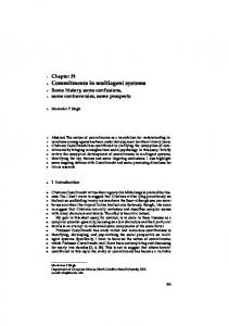
Figure 2: New architecture of a bounded rational agent

rationality in agent control. The classic architecture is augmented with a meta-level control component and there are various options for invoking the scheduling and coordination components. These options differ in their resource usage and performance. The meta-level control component will decide if, when and how much control activity is necessary for each event sensed by the agent. Meta-level control activities optimize the agent’s performance by choosing and sequencing domain and control activities. This includes allocating appropriate amount of processor and other resources at appropriate times. If significant resources are expended on making this meta-level control decision, then the meta-meta-level decisions have to be made on whether to spend these resources on meta-level control. To do this an agent would have to know the effect of all combinations of actions ahead of time, which is intractable for any reasonably sized problem. The question of how to approximate this ideal of sequencing domain and control activities without consuming too many resources in the process, is the meta-level control problem for a resource bounded rational agent.

1.1 Assumptions The following assumptions are made in the solution described in this proposal: The agents are cooperative and will prefer alternatives which increase social utility even if it is at the cost of decreasing local utility. However, the solution approach proposed and developed in this document generalizes to self-interested environments as well. This is discussed further in Section 2. An agent may concurrently pursue multiple high-level goals and the completion of a goal derives utility for the system or agent. The overall goal of the system or agent is to maximize the utility generated over some finite time horizon. Quality and Utility are equivalent measures of performance in this system. The high-level goals are generated by either internal or external events being sensed and/or requests by other agents for assistance. These goals must often be completed by a certain time in order to achieve any utility. It is not necessary for all high-level goals to be completed in order for an agent to derive utility from its activities. The partial satisfaction of a high-level goal is sometimes permissible while trading-off the amount of utility derived for decrease in resource usage. The agent’s scheduling decisions involve choosing which of these high-level goals to pursue and how to go about achieving them. There can be non-local and local dependencies between tasks and methods. Local dependencies are inter-agent while non-local dependencies are intra-agent. These dependencies can be hard or soft precedence relationships. Coordination decisions involve choosing the tasks which require coordination and also which agent to coordinate with and how much effort much be spent on coordination. Scheduling and coordination activities do not have to be done immediately after there are requests for them and in some cases may not be done at all. There are alternative ways of completing scheduling and coordination activities which trade-off the likelihood of these activities 4

resulting in optimal decisions versus the amount of resources used.

1.2 Agent Decision Space There are two types of decisions made by an agent: the meta or macro-level decisions handled by the meta-level controller and the scheduling or micro-level decisions handled by the domain-level controller. Figure ?? describes the hierarchy of decisions. The meta-level controller will be designed to make quick and inexpensive decisions on how much resources should be spent on domain versus control actions. The initial control decisions are further classified into three types: Coordination decisions, which decide whether or not to coordinate with other agents and how much effort should be spent on coordination Scheduler decisions, which dictate whether or not to call the domain-level scheduler and how much effort should be spent by the scheduler Slack decisions which will prescribe how much total slack/free time should be included in a schedule to deal with unexpected events. In this work, coordination is the inter-agent negotiation process that establishes commitments on completion times of tasks or methods. An example of a coordination meta-level decision is determining how long a negotiation should take. If an agent decides to negotiate, it should also decide whether to negotiate by means of a single step or a multistep protocol that may require a number of negotiation cycles to find an acceptable solution or even a more expensive search for a near-optimal solution. The benefit of choosing a more expensive protocol is that social utility is more likely to be higher as a result of successfully completing the negotiation as expected. The cost involved is that more resources are invested on negotiation and delays in the execution of domain tasks since domain tasks facilitated by the negotiation cannot execute until the negotiation is completed. The high-level goal of this work is to create agents which can maximize the social utility by successfully completing their goals. These agents also necessarily have limited computation and detailed models of the task environments are not readily available. Reinforcement learning is useful for learning the utility of these control activities and decision strategies in such contexts. This naturally leads to the construction of a MDP-based meta-level controller which uses reinforcement learning techniques to approximate an optimal policy for allocating computational resources. This approach to meta-level control implicitly deals with opportunity cost as a result of the long-term effects of the meta-level decisions on utility. [31] states that the opportunity cost of a decision arises because choosing one thing in a world of scarcity means giving up something else. Opportunity cost is defined as the value of the good or service foregone. This means the choice of the meta-level controller of one task over another, due to deadline and other resource constraints, contains an implied opportunity cost. A basic assumption of my approach is to build a meta-level controller for a specific environment which has a welldefined set of agents, tasks and arrival models of tasks, rather than handle any arbitrary environment. In order to make effective meta-level decisions, agents have to develop a good model of the opportunity cost of performing actions. The accuracy of the agent’s analysis of the down-stream effects of various meta-level choices depends on the accuracy of the opportunity cost model. Due to the complex interactions among tasks and agents in the problem environments, an accurate opportunity cost model can be constructed only with respect to specific environments. We plan to generate a library of specific environments and their corresponding policies. We will analyze the characteristics of different environments which share the same policy to gather insight on partitioning the space of task environments. The search space for each environment is represented using factored Markov Decision Processes(MDPs). Factored MDPs are compact representations of MDPs using Bayesian Networks.

1.3 Proposed Agent Architecture The following is an overview of my approach for providing effective meta-level control for resource-bounded agents. We begin by describing the detailed architecture of a resource-bounded agent that uses offline policies built using reinforcement learning. It is a detailed variant of the high level architecture described in Figure 2. I will enumerate the characteristics of the policy that allows the agent to dynamically react to real-time unanticipated exogenous events. 5

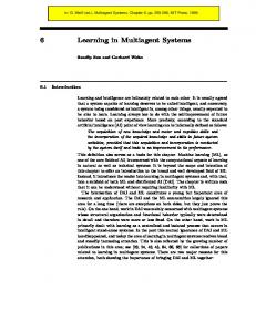
We also discuss how the overhead associated with meta-level control and control activities is explicitly costed out. Section 2 describes the approach in further detail. Our aim is to validate the following thesis. Thesis Statement: Approximating the ideal solution to meta-level decisions made by individual agents in a cooperative multi-agent system, using reinforcement learning methods, provides effective allocation of computation and improved performance. Figure 3 illustrates a conceptual architecture of a resource-bounded agent that uses offline-learning for meta-level control. The number sequences describe the steps in a single flow of control. At the heart of the system is the Domain Problem Solver(DPS). It receives tasks and other external requests from the environment(Step 1). When an exogenous event such as arrival of a new task occurs, the DPS sends the corresponding task set, resource constraints as well constraints of other tasks which are being executed, and performance criteria to the meta-level controller(Step 2). The controller computes the corresponding state and determines the best action prescribed by the policy which has been computed offline for that particular task environment. The best action can be to call one of the two domain schedulers on a subset of tasks, to gather more information to support the decision process, to drop the new ask or to do nothing. The meta-level controller then sends the prescribed best action back to the DPS(Step 2a). The DPS, based on the exact nature of the prescribed action, can invoke the complex scheduler, simple scheduler(abstraction component) or coordination component(Step 3) and receives the appropriate output(Step 3a). If the action is to invoke the complex scheduler, the scheduler component receives the task structure and criteria as input and outputs the best satisficing schedule as a partially ordered sequence of primitive actions. The complex scheduler can also be called to determine the constraints on which a coordination commitment is established. If the meta-level or the domain scheduler prescribe an action that requires establishing a commitment with a non-local agent, then the coordination component is invoked. The coordination component receives a vector of commitments that have to be established and outputs the status of the commitments after coordination completes. The simple scheduler or abstraction component is invoked by the DPS and receives the task structure and goal criteria. It then sends the appropriate pre-computed schedule which fits the criteria. The DPS can invoke the execution component either to execute a single action prescribed by the meta-level controller or a schedule prescribed by the domain-level scheduler(Step 4). The execution results are sent back to the DPS(Step 4a) where they are evaluated and if the execution performance deviates from expected performance, the necessary measures are taken by the DPS. The features and functionality of the individual components are discussed in detail in Section 2. This work accounts for the cost of all three levels of the decision hierarchy - meta-level control, control and domain activities. Meta-level control involves reasoning about the cost of negotiation and scheduling activities. The cost of this reasoning is accounted for directly within the MDP framework. Negotiation costs are reasoned about explicitly in my framework because they are modeled as part of the domain activities needed to complete a high-level goal. We will discuss this further in Section 2. The negotiation tasks are split into an information gathering phase and a negotiating phase, with the outcome of the former enabling the latter. The negotiation phase can be achieved by choosing two members from a family of negotiation protocols[51]. The information gathering phase is modeled as a MetaNeg method in the task structure and the negotiation methods are modeled as individual primitive actions. Thus, reasoning about the costs of negotiation is done explicitly, just as it is done for regular domain-level activities. The MetaNeg method belongs to a special class of domain actions which request an external agent for a certain set of information and it does not use local processor time. It queries the other agent and returns the following information: < Expe tedUtility; Expe ted ompletiontime; Sla kAmount >. This information is used by the meta-level controller to determine the relevant control actions. However, reasoning about the time cost associated with scheduling of unanticipated exogenous events is implicit. This is because time is not represented explicitly in the MDP. The passage of time will change state features which will in turn cause the system to account for time used in scheduling and the generation of complex features. Slack in the execution policy provides flexibility for the policy to dynamically react to unexpected events. The flexibility is built-in at the cost of diminished expected performance characteristics. Specifically, slack affects the crispness in overall expected performance of the system as well as opportunistic tendencies of the system. A crisp schedule is efficient within the myopic context for which it is initially computed and does not account for any external events. Opportunism is proportional to the amount of slack in the schedule while performance crispness is inversely proportional to slack amount. To handle unexpected exogenous events, the system learns to estimate when to allocate 6

Meta-Level Control Component

2a

2 *Domain Tasks *Constraints *Goal Criteria

*Best action

1 Simple domain scheduler

Environment

3 *Goal Criteria 3a*Schedule 3 *Goal 3a Criteria

*New tasks *Goal Criteria

Domain Problem Solver

3a

3

* Neg. Constraints

4a *Feedback

*Action/ *Commitments Schedule

*Schedule

Complex Domain Scheduler

4

Coordination Component

Execution and Monitoring Component

Figure 3: Conceptual architecture of a bounded rational agent

slack and how much slack to allocate. The domain level scheduler depicted in the architecture will be an extended version of the Design-to-Criteria(DTC) scheduler[46]. Design-to-Criteria (DTC) scheduling is the soft real-time process of finding an execution path through a hierarchical task network such that the resultant schedule meets certain design criteria, such as real-time deadlines, cost limits, and quality preferences. It is the heart of agent control in agent-based systems such as the resource-Bounded Information Gathering agent BIG [20] and the multi-agent Intelligent Home [21] agent environment. Casting the language into an action-selecting-sequencing problem, the process is to select a subset of primitive actions from a set of candidate actions, and sequence them, so that the end result is an end-to-end schedule of an agent’s activities that meets situation specific design criteria. The DTC scheduler will be augmented as described in Section 2 to meet the requirements of this problem domain. The abstraction component also described in Section 2 and will support reactive control for highly constrained situations.

1.4 Taxonomy of meta-level decisions A formal description of the problem is given in the appendix. We will now describe a taxonomy of meta-level decisions in a multi-agent system using the simple example scenario. There are five types of exogenous events that require metalevel decision making 1. arrival of a new task from the environment 2. presence of a non-locally enabled task in the current task set that could lead to negotiation with a non-local agent 3. failure of a negotiation to reach a commitment 4. invoking the domain scheduler to schedule a new set of tasks or to reschedule existing tasks 5. significant deviation of online schedule performance from expected performance In order to provide a clear picture of these five decisions, consider the simple scenario described in the previous subsection consisting of 2 agents A and B. The discussion will specifically focus on the various meta-level questions that will have to be addressed by agent A. Figure 4 describes T0 and T1, which are the tasks performed by agent 7

A. They are described using TÆMS, a domain independent framework for describing task structures. A detailed description of TÆMS and its features is provided in the appendix.

Agent A: T0

T1

sum

sum M1 Q 100% 6 D 100% 8

M2

M3 Q 100% 12 D 100% 8

Q 90% 10 10% 12 D 90% 10 10% 12

M4 Q 90% 10 10% 12 D 90% 10 10% 12 enables from N5

enables to N4

Figure 4: Tasks that can be performed by agent A In this example, each top-level task is decomposed into two executable primitive actions. In order to achieve the task, agent A can execute one or both of its primitive actions within the task deadline and the quality accrued for the task will be cumulative (denoted by the sum function). The enables relationship from method M1 of task T0 to a non-local method N4 of task S1 belonging to agent B (agent B’s task structure is not shown) implies that successful execution of M1 is a precondition for executing N4. The following are some of the specific meta-level questions that will be addressed by any individual agent. Each meta-level question is followed by a description of agent A’s perspective of each question and the associated costs and benefits. We also enumerate some of the factors we think will be relevant in making the individual decisions. Coordination execution: 1. Should a local method which is enabled by a non-local method be included in the agent’s schedule? Meta-Level Question: Should method M4, which is enabled by agent B’s method N5, be included in the agent A’s schedule? Benefit: If method M4 is included in agent A’s schedule, agent A can increase its total utility. Cost: This implies that agent A and B have to negotiate over the completion time of method N5 by agent B and this will take time. (a) Does the task with enabled method have high priority (method has a high utility and a a relatively close deadline) ? (b) Does the alternative that achieves the goal without coordination, if it exists, have significantly lower utility than the alternative that involves coordination? (c) Does the utility of the task offset the cost of coordination? 2. Should the local enabler with a non-local enablee be included in the agent’s schedule? Meta-Level Question: Should method M1, which enables agent B’s method N4, be included in agent A’s schedule? Benefit: If agent B’s method N4 is enabled by agent A, then agent B will increase its total utility causing the social utility to increase. Cost: This implies that agent A and B have to negotiate over the completion time of method M1 by agent A and also that agent A is bound to the commitment results from the negotiation. The costs in this case are time for negotiation and loss of local autonomy, specifically, Agent A is not as flexible to accomplish its local goals if it commits to a completion time for method M1. 8

(a) Is there a high probability that the non-local agent will request the enabler to be executed? (b) Is the schedule relatively flexible(low load) to include the enablee even if it does not contribute towards achieving the local goals? (c) Is the local enabler capable of achieving current local goals, so that cooperative goals can be piggybacked with local goals? Coordination effort: 1. How long should coordination take? Meta-Level Question: If agent A decides to negotiate, it should also decide whether to negotiate by means of a single step or a multi-step protocol that may require a number of negotiation cycles to find an acceptable solution or even a more expensive search for a near-optimal solution. For example, should a single shot protocol which is quick but has a chance of failure be used or a more complex protocol which takes more time and has a higher chance of success. Benefit: If agent A receives high utility as a result of completing negotiation on finish time of N5, then better the protocol, the higher the probability that the negotiation will succeed. Cost: The protocols which have a higher guarantee of success require more resources, more cycles and more end-to-end time in case of multi-step negotiation and higher computation power and time in case of near-optimal solutions. (The end-to-end time is proportional to the delay in being able to start task executions). (a) How important is coordination to achieving the desired task? (b) How dependent are local tasks on the negotiated task? (c) How does the expected task utility drop off if the coordination option is replaced by an option requiring no coordination? (d) How tight is the current schedule? 2. Can the negotiation be restarted with the same agent or an alternate agent, if the previous negotiation fails? If so, how many such restarts? Meta-Level Question: If the negotiation between agents A and B using a particular negotiation protocol fails, should agent A retry with the same mechanism or an alternate mechanism; with the same agent or alternate agents and how many such retries should take place? Benefit: If negotiation is preferred (agent A will receive high utility as result of completion of N5), there there is a higher chance of negotiation succeeding if more time(cycles) is given. Since resources have been spent on figuring out a solution to the negotiation, it may be profitable to put in a little more effort and achieve a solution. Cost: This implies that agent A and B have to negotiate over the completion time of method N5 by agent B and this will take time and computational resources. If there is a very slight or no probability of finding an acceptable commitment, then resources which can be profitably spent on other solution paths are being wasted and the agent might find itself in a dead-end situation with no resources left for an alternate solution. (a) Are there enough resources to renegotiate? Domain-level Scheduler execution: 1. Should the agent do detailed scheduling-related reasoning about an incoming task at arrival time or later or never? Meta-Level Question: Should agent A schedule newly arriving task Tx at arrival time or postpone scheduling to sometime in the future or drop that particular instance of the task. Benefit: If the new task has very low or negligible priority and high opportunity cost, then it should be discarded. If the incoming task Tx has very high priority, in other words, the expected utility is very high and it has a relatively close deadline, then the agent should override its current schedule and schedule the new task immediately. If the current schedule has average utility that is significantly higher than the new task and the average deadline of the current schedule is significantly closer than that of the new task, then 9

reasoning about the new task should be postponed till later. Cost: If the new task is scheduled immediately, the scheduling action costs time, and there are associated costs of dropping established commitments if the previous schedule is significantly revised or completely dropped. These costs are diminished or avoided completely if the task reasoning is postponed to later or completely avoided if the task is dropped. (a) What is the priority of the incoming task? (b) What is the average priority of the current task set? (c) How tight is the current schedule? 2. Should a reschedule be called when current performance deviates from expected performance? If so, what’s the deviation threshold limit above which a reschedule should be initiated? Meta-Level Question: When agent A’s schedule deviates from expected performance by threshold , should a reschedule be invoked automatically? Benefit: If the agent observes that the schedule will fail to achieve its goal in a timely fashion, then it can reschedule and try an alternate path instead of going down a path which will definitely fail. Cost: There is a cost associated with calling the scheduler and revising the commitments from the previous schedule. (a) What is the loss in utility and is the reschedule overhead worth the effort? Domain-level Scheduler effort: 1. How many resources should be invested in reasoning about an incoming task at arrival time? Meta-Level Question: When agent A’s scheduler is called, it has to decide how much effort it should put in scheduling. Benefit: If the expected schedule performance characteristics are highly uncertain, then it is better for the scheduler to put in less effort and look at shorter horizons. Cost: If the scheduler looks at short horizons, there is a cost associated with the subsequent rescheduling calls. Also, the myopic view of the schedule in the short-horizon case leads to less optimal schedules. However if the scheduler is called only once with a distant horizon parameter, but the schedule performance is not as expected, then rescheduling has to be called anyways and the system might put itself in a dead-end with no resources to find an alternate solution. This means a trade-off on the number of reschedule calls and effectiveness of these calls has to be made. (a) What is the scheduling horizon, specifically how far ahead into the future should the scheduler consider when making a detailed schedule? The options are immediate(short term) and distant (long term) horizon1 (b) Should it involve rescheduling only the incoming task and subsequent fitting of this new task in preexisting schedule or should all currently scheduled tasks and the new task be rescheduled or should the new task be delayed till current schedule is completed? (Suppose task T0 arrives at agent A while it is executing schedule X. Should the scheduler be invoked for only task T0 and the resulting method sequence be fit into X, or should task T0 and unexecuted tasks in X be rescheduled and a new schedule X prime be produced or should scheduling of task T0 be delayed till X is completed?) 2. Slack Issues: How flexible should the schedule produced by the detailed scheduler be? Should it be tight since the tasks are high priority with tight deadlines or loose since the current tasks are of low priority and there is a significant probability of arrival of a new high priority task. 1 two horizon categories are chosen for the sake of simplicity. The number of horizons used by the system at real-time can be adjusted and will be dependent on the problem characteristics.

10

Meta-Level Question: How much slack should be inserted in the schedule? Benefit: If there is slack in the schedule, then the system can deal with unanticipated events easily without having to bear the overhead of a reschedule. Cost: Inserting slack in the schedule means that fewer primitive actions that have to be done will be scheduled causing the available time to not be used to maximum capacity. Here, the level of execution towards current goals is being traded-off to provide resources for unanticipated future events. The domain-level controller, on the other hand, has an associated resource overhead and will receive directives from the meta-level controller on when to execute and how much effort to put in its execution. These are some of the specific questions addressed by the domain-level scheduler 1. How to allocate resources to individual primitive actions? 2. When is it most appropriate to include slack in the schedule/policy to allow meta-level reasoning of unanticipated events? 3. How to best use slack time available from negotiation. i.e. the time spent waiting for response from the other agent? The remainder of this document is structured as follows: The solution approach along with a detailed example to motivate the work is described in Section 2. The anticipated contributions of the thesis are enumerated in Section 3. Section 4 provides an overview of the current state of the art research on meta-level reasoning in multi-agent system. Section 5 describes the work plan and criteria for evaluating the system.

2 Solution Approach This section describes in detail the meta-level component introduced in Figure 3. First we discuss why reinforcement learning is an appropriate solution approach for meta-level control. I then describe the states and actions of the underlying Markov Decision Process used by the learning component, including the details of the state features. We then present snapshots of the meta-level reasoning process using a MDP for specific exogenous events which are represented in the system state. We finally use an example to illustrate the functionality of the infrastructure that has been constructed in the previous sub-sections. The high-level goal of this work is to build a framework which will support an agent in learning an optimal metalevel control behavior policy, given a specific task environment. The motivation for such a component was described in Section 1. The absence of a model of the dynamic and highly non-deterministic environment makes learning and adaptation key to obtaining good system performance. They are essential for developing meta-level control strategies that meet the demands of the environment and the requirements of individual agents. Reinforcement Learning is an effective paradigm for training an agent to act in its environment in pursuit of a goal. For the purposes of this research, the learning will be done off-line. The only reason that it is not done online is because it is a much longer process. The learning component will learn to make decisions such as when a new task should be accepted/delayed/rejected, when it is appropriate to renegotiate when a negotiation task fails and how much effort to put into scheduling when reasoning about a new task. At a more abstract level the system would also learn the correlation and co-occurrence of tasks. It will also learn characteristics which predict the behavior and reliability of other agents for varying loads and deadline constraints. A related area for future research is to alter the assumptions of the environment such that a statistical model of task arrival is available to the agent. It will be interesting to investigate how the decision-making process of the agent will be modified by the availability of this information.

Problem Representation: We model this sequential decision making process using a structured MDP which represents the dynamics of the underlying search space. The system state is captured by the state of the MDP. In many cases it is advantageous, from both the representational and computational point of view, to talk about properties of states or sets of states: 11

the set of possible initial states, the set of states in which an action can be executed, and so on. It is generally more convenient and compact to describe sets of states based on certain properties or features than to enumerate them explicitly. Representations in which descriptions of objects substitute for the objects themselves are called intensional and is the technique of choice in AI systems [3]. An intensional representation for planning systems is often built by defining a set of features that are sufficient to describe the state of the dynamic system of interest. A structured MDP is an intensional representation. The fundamental tradeoff between extensional and intensional representations becomes clear when the former views the space of possible states as a single variable that takes on 100’s of possible values, whereas the intensional or factored representation views a state as the cross product of n variables, each of which takes on substantially fewer values. Generally, the state space grows exponentially in the number of features required to describe a system. Meta-level control activities can be costed out by accounting for the overhead of state feature computation. Hypothetically, the features of MDP state enumerated in Figure 5 are needed to make effective meta-level control decisions. These are intuitive features that we think will support the system’s decision making process and may evolve over time as we study their effectiveness through experimentation. There are thirteen features, which are of two categories - simple features where the reference values are readily available by simple lookups and complex features which involve significant amount of computation to determine their values. Using the MDP, the system make explicit decisions whether to gather complex features and determine which complex features are appropriate. The cost of gathering these features will be implicitly represented in the MDP by the time information within the complex feature. This implies that an estimate for computing the complex feature is made and the feature is computed such that it is valid when the computation is completed. The decision on whether to compute the complex features constitute the meta-meta-level decisions mentioned in the introduction. The simple features are inexpensive to compute since they are based on average statistics. These features help the agent make informed decisions on executable actions or whether to obtain more complex features to make the decisions. An example of a simple feature would be the availability of slack in the current schedule(F4). If there is a lot of slack or too little slack, the decision to accept the new task or drop the new task respectively is made. However, if there is a moderate amount of slack, the agent might choose to obtain a more complex feature, namely F12 described below. The complex features are usually context-sensitive and involve computations that take time that is sufficiently long that, if not accounted for, will lead to incorrect meta-level decisions. Context-sensitivity makes the computation of the features cumbersome since they involve determining detailed timing, placement and priority 2 characteristics and provide the meta-level controller with information to make more accurate action choices. For instance, instead of having a feature which gives a general description of the slack distribution in the current schedule i.e. there is a lot of slack in the beginning or end of the schedule, there is a feature(F12) which examines the exact characteristics of the new task and makes a determination whether the available slack distribution will likely allow for a new task to be included in the schedule.

Utility Function: This work focuses on cooperative multi-agent systems where agents prefer alternatives which increase social utility even if it is at the cost of decreasing their local utility. The rewards are computed from a single agent perspective for a given episode/time bound. We assume that agents will receive individual intermediate rewards instantaneously when assigned tasks are accomplished. We diverge from the commonly used cumulative reward model where the reward for each agent is a function of the sum total of the rewards of all the agents in the multi-agent system at the end of the episode . Previous works [5, 4, 35] have used the cumulative reward functions in cooperative environments. There are two problems with these reward functions. The first is that they ignore the costs incurred by computing and communicating the rewards of each of the agents. The second problem is that credit assignment is very approximate and a large number of learning trials are required for the assignments to converge to the right values. We will also incorporate a notion of social consciousness to the reward using a function similar to the brownie point model described in [9]. Agents will receive rewards for accomplishing the individual tasks and for performing actions which benefit social utility rather than local utility. 2 priority accounts for quality and deadline

12

When designing any agent-based system, it is also important to determine the level of sophistication of the agents’ reasoning process. Reactive agents simply retrieve pre-set behaviors similar to reflexes without maintaining any internal state. On the other hand, deliberative agents behave more like they are thinking, by searching through a space of behaviors, maintaining internal state, and predicting the effects of actions. Although the line between reactive and deliberative agents can be somewhat blurry, an agent with no internal state is certainly reactive, and one which bases its actions on the predicted actions of other agents is deliberative.

Levels of reactivity: This architecture supports a hybrid of reactive and deliberative behaviors. The agent will learn when to be reactive and when to do significant deliberation on what to do next. In this case, internal state is always maintained but the difference will be in the extent to which this internal state is used. If detailed internal state and the associated feature computation is required, then the agent exhibits deliberative behavior else its is reactive. The system has levels of reactivity/deliberation trade-offs available as options. As mentioned in Section 1, the domain-level scheduler will be an extension of the Design-to-Criteria scheduler. DTC will be augmented to construct partially-ordered schedules for tasks that achieve the high-level goal while adhering to the design criteria and constraints like hard deadlines or limits on negotiation times. This decision problem requires a sophisticated approach because of the task’s inherent computational complexity and has an associated cost. The DTC scheduler will be augmented to handle parameters like schedule horizon and scheduler effort which will control its execution overhead. This is to support varying levels of deliberation in the system. To facilitate reactive control, we will build a task structure abstraction component. The abstraction component will be a cheaper alternative to the DTC scheduler. Abstraction is an offline process where potential schedules and their associated performance characteristics for achieving the high level tasks are discovered for varying objective criteria. This is achieved by systematically searching over the space of objective criteria. Also multiple schedules could potentially be represented by the same abstraction. The abstraction component will hide the details of these potential schedules and will provide only the high level information necessary to make meta-level choices. When an agent has to schedule a task but doesn’t have the resources or time to call the domain-level scheduler, the generic abstraction information of the task structure can be used to provide the approximate schedule. The abstraction component contains abstraction for each of the task structures in the problem environment. Each entry in the table is the schedule sequence and performance characteristics for the task structure given a certain objective criteria.

2.1 Description of State features

FeatureID F0 F1 F2 F3 F4 F5 F6 F7 F8 F9 F10 F11 F12

Feature Current status of system Relation of quality gain per unit time of a particular task to that of currently scheduled task set Relation of deadline of a particular task to that of currently scheduled task set Relation of priority of items on agenda to that of currently scheduled task set Percent of slack in local schedule Percent of slack in other agent’s schedule Relation of priority of non-local task to non-local agent’s currently scheduled task set Expected Quality of current item at time t Actual Quality of current item at time t Expected Rescheduling Cost with respect to a task set Expected DeCommitment Cost with respect to a particular task Relation of slack fragments in local schedule to new task Relation of slack fragments in non-local agent to non-local task

Figure 5: Table of proposed state features, their description and category

13

Complexity Simple Simple Simple Simple Simple Simple Simple Simple Simple Simple Complex Complex Complex

The search space of the meta-level controller is described using a factored MDP, where each state has a set of features. The following is a detailed description of the characteristics and computations involved in each of the state features described in Figure 5: There are twelve features, ten of which have 4 different feature values and two have two values each. So the maximum size of a search space is 41 0  22 = 222 , which is about a million states. F0: Current state of the system which is represented as a 4-tuple:

< NewItemsList; Agenda; S heduleList; Exe utionList > where each entry in the tuple contains the number of items on the corresponding list. The new items are the tasks which have just arrived at the agent from the environment. This feature is computed for all exogenous events. The agenda list is the set of tasks which have arrived at the agent but their reasoning has been delayed. They have not been scheduled yet. The schedule list is the set of tasks to be executed. The execution list is the set of primitive actions which have been scheduled to achieve the top level tasks and maybe in execution or yet to be executed. Eg. < 2; 0; 0; 1 > means there are two new items which have arrived from the environment and there is one task in execution. F1: Relation of utility gain per unit time of a particular task to that of currently scheduled task set The utility gain per unit time of a task is the ratio of total expe ted utility to total expe ted duration of that task. This feature compares the utility of a particular task to that of the existing task set and helps determine whether the new task is very valuable, moderately valuable or not valuable in terms of utility to the local agent. This feature is also computed the following exogenous events occur: Arrival of new task and Domain-level scheduler is invoked. The feature value is an integer and can be one of the following 0 : default value. 1 : relative quality gain of new task is very high 2 : relative quality gain of new task is moderate 3 : relative quality gain of new task is low F2: Relation of deadline of a particular task to that of currently scheduled task set This feature compares the deadline of a particular task to that of the existing task set and helps determine whether the new task’s deadline is very close, moderately close or far in the future. This feature is computed when the following exogenous events occur: Arrival of new task and Domain-level scheduler is invoked. The feature value is an integer and can be one of the following 0 : default value. 1 : relative deadline of new task is very close 2 : relative deadline of new task is moderate 3 : relative deadline of new task is far-off F3: Relation of priority of items on agenda to that of currently scheduled task set This feature compares the average priority of the existing task set to the priority of the new task and helps determine whether the new task is very valuable, moderately valuable or not valuable in terms of utility to the local agent. Priority is a function of the utility and deadlines of the tasks. It is my intuition that computing the average priority of a task set is a more complicated function than computing the priority of a single tasks since it involves recognizing dominance of individual tasks. This feature is computed when the following exogenous events occur: There are items on the agenda when arrival of new task and Domain-level scheduler is invoked. The feature value is an integer and can be one of the following 0 : default value. 1 : items on agenda have very high priority. 2 : items on agenda have very medium priority. 3 : items on agenda have very low priority. 14

F4: Percent of slack in local schedule This feature is used to make a quick evaluation of the flexibility in the local schedule. This feature is computed when the following exogenous events occur: Presence of non-locally enabled task in current task set, Failure of a negotiation to reach a commitment , Domain-level scheduler is invoked and Online performance deviates from expected performance. The feature value is an integer and can be one of the following 0 : default value. 1 : Local schedule has high slack. 2 : Local schedule has medium slack. 3 : Local schedule has low slack. F5: Percent of slack in other agent’s schedule This feature is used to make a quick evaluation of the flexibility on the other agent’s schedule. The computation of feature F5 is inexpensive since it is done after an information gathering phase, represented by a primitive action called MetaNeg, (see Figure 8) which when executed will gather information on non-local agents which are potential coordination partners for the local agent. This feature is computed when the following exogenous events occur: Presence of non-locally enabled task in current task set and Failure of a negotiation to reach a commitment.The feature value is an integer and can be one of the following 0 : default value. 1 : Other agent’s schedule has high slack. 2 : Other agent’s schedule has medium slack. 3 : Other agent’s schedule has low slack. F6: Relation of utility gain per unit time of non-local task to non-local agent’s current task set This feature compares the utility of a particular task to that of the existing task set of a non-local agent and helps determine whether the new task is very valuable, moderately valuable or not valuable with respect to the utility of the other agent. The computation of feature F6 is inexpensive since it too is done after the information gathering phase. This feature is computed when the following exogenous events occur: Presence of non-locally enabled task in current task set and Failure of a negotiation to reach a commitment. The feature value is an integer and can be one of the following 0 : default value. 1 : Task with non-local effect has high utility. 2 : Task with non-local effect has medium utility. 3 : Task with non-local effect has low utility. F7: Expected utility of current schedule item at current time This is the expected utility of the current schedule item at time t as determined by the domain-level scheduler which uses expected value computations. This feature is computed when the following exogenous event occurs: Failure of a negotiation to reach a commitment and Online performance deviates from expected performance. This is a real value denoting the expected utility of the primitive action upon execution. F8: Actual utility of current schedule item at current time This is the actual quality of the current schedule item at run time t. This feature is compared to F7 in order to determine whether schedule execution is proceeding as expected. This feature is computed when the following exogenous event occurs: Failure of a negotiation to reach a commitment and Online performance deviates from expected performance. This is a real value denoting the actual utility of the primitive action upon execution. F9: Expected Rescheduling Cost with respect to a task set This feature estimates the cost of rescheduling a task set and it depends on the size and quality accumulation factor of the task structure. It also depends on the horizon and effort parameters specified to the domain-level 15

scheduler. This feature is computed when the following exogenous events occur: Arrival of new task, Failure of a negotiation to reach a commitment and Domain-level scheduler is invoked. The feature value is an integer and can be one of the following 0 : default value. 1 : Rescheduling cost is high 2 : Rescheduling cost is medium 3 : Rescheduling cost is low F10: Expected DeCommitment Cost with respect to a particular task This is a complex feature which estimates the cost of decommiting from a method/task by considering the local and non-local down-stream effects of such a decommit. The domain-level could be invoked a number of times in order to compute this feature. It is computed when the following exogenous events occur: Arrival of new task, Domain-level scheduler is invoked. The feature value is an integer and can be one of the following 0 : default value. 1 : Decommitment cost is high 2 : Decommitment cost is medium 3 : Decommitment cost is low F11: Relation of slack fragmentation in local schedule to new task This is a complex feature which determines the feasibility of fitting a new task given the detailed fragmentation of slack in a particular schedule. It involves resolving detailed timing and placement issues. This feature is computed when the following exogenous events occur: Presence of non-locally enabled task in current task set, Failure of a negotiation to reach a commitment and Domain-level scheduler is invoked. The feature value is an integer and can be one of the following 0 : default value. 1 : feasibility of fitting task locally is high 2 : feasibility of fitting task locally is medium 3 : feasibility of fitting task locally is low F12: Relation of slack fragments in non-local agent to non-local task This is a complex feature which determines the feasibility of fitting a new task given the detailed fragmentation of slack in a particular non-local schedule. It involves resolving detailed timing and placement issues. This feature is computed when the following exogenous events occur: Presence of non-locally enabled task in current task set and Execution of MetaNeg completes. The feature value is an integer and can be one of the following 0 : default value. 1 : feasibility of fitting task non-locally is high 2 : feasibility of fitting task non-locally is medium 3 : feasibility of fitting task non-locally is low

2.2 Exogenous Events and Related Actions There are five situations where meta-level reasoning is desirable 1. decision of what to do with a new task when it arrives 2. decision on whether to initiate negotiation 3. decision on whether to renegotiate in the event of a renege 4. decision on amount of scheduler effort 16

Wait State

Decision Tree for new task (Figure 7)

Decision Tree for Reschedule (Figure 11)

Decision Tree for negotiation (Figure 8) Decision Tree for schedule execution (Figure 10)

Decision Tree for renegotiation (Figure 9)

Active Execution State

Figure 6: FSM describing interactions among high level states of an agent

5. decision to spontaneously reschedule based on execution characteristics In this section, we describe the choices available to the agent in each of these situations and the approximate criteria for making the choice. Each event is described as an external action in a decision tree. The external action triggers a state change. The response actions (executable or parameter determining) are also modeled in the decision tree. For the sake of clarity, every leaf in the decision tree is marked by an identifier and referenced by the associated text description. The finite state machine (FSM) described by Figure 6 gives a birds-eye view of the interaction among the seven possible high-level states of an agent. Five of these states represent the decision trees for the five exogenous events. The other two states are Active Execution State and Wait State which are primitive states. Active Execution State represents the state when the agent is actively using the processor to execute a scheduled domain-level action. Wait State represents the state when the agent is waiting for an exogenous event to occur. The other five states are abstractions of the meta-level decisions that need to be made as a consequence of exogenous events. The possible termination states determine their interactions with the primitive actions. For instance, an agent in initial waiting state moves to another state only as a consequence of the arrival of a new task. An agent in Active Execution State can be interrupted by any one of the five meta-level decisions and any of the meta-level decisions could lead to a transition to the waiting state. The FSM serves as a template for generating the MDP for which the optimal policy is computed using reinforcement learning. The FSM for each task environment is a sequential combination of the expanded decision trees for the exogenous event states as they occur over time. Specifically, for each task environment with an arrival model the MDP is built incrementally from a start state by augmenting the decision tree associated to the exogenous events as they occur. Every terminal state of a decision tree transitions to the starting state of the decision tree representing the decision process of the next exogenous event. The states of the policy dynamically constructed by the agent are described in the mini-MDPs associated with each of the meta-level decisions. The number of states in a typical problem instance is the subject of current research. The state transition probabilities caused by exogenous events as well action completions will be learned for each situation. The following are not decision rules learned by the system. Instead, I have hand-crafted some intuitive decision rules that could be approximations of the actual rules learned by the system. 17

Drop task

Use simple scheduler on new task New task

[A1]

[A2]

Use detailed scheduler [A3]

arrives

on new task Use detailed scheduler on all tasks including [A4] partially executed tasks Add new task [A5]

Legend

to agenda

Use detailed [A7]

Drop new task

state

and drop agenda

[A6]

scheduler on task

executable action external action transition function

Get new features

Add task

[A8]

to agenda Drop task [A9]

Figure 7: Decision tree when a new task arrives

1. Decision Tree for New Task (Figure 7): Exogenous Event: Arrival of a new task Action: Decision of what to do with a new task Suppose a new task Tx arrives at time t. The agent has to decide whether to delay the reasoning about scheduling task Tx till later; never execute the task; execute the task immediately at arrival time by calling for a reschedule action or add the new task to the agenda. If more than one new task arrives at time t, the set of new tasks are considered as one new task under a sum. Alternatively, the tasks can be evaluated individually based on some criteria such as priority. We discuss it further later on this section. The reinforcement learner will learn to choose an action from the above-mentioned action choices. The corresponding decision tree is described in Figure 7 and an intuitive view of the reasoning process required to support each of the action choices is described below. (a) Drop task and revert to original status [A1]: If utility of the new task Tx is really low and quality of current task set is relatively high or the deadline of task Tx is too close to even attempt to do the task, then drop the task with no reconsideration. The agent reverts back to the Active Execution or Wait State it was in before it was interrupted by the exogenous event. Possible features used are F0, F1, F2. (b) Do task now using simplescheduling i.e. abstraction-based alternative selection and call execution component[A2]: If utility of new task Tx is very high, its deadline is so close that detailed scheduling is not possible, the utility of current scheduled task set is significantly low, then do new task now with the metalevel controller choosing an alternative that best fits the objective criteria. Possible features used are F0, F1, F2. 18

(c) Do task now using complex domain-level scheduler [A3]: If utility of new task Tx is very high, its deadline is close but far enough to allow detailed scheduling of the single task, the utility of current scheduled task set is significantly low, then do new task now with the meta-level controller choosing an alternative that best fits the objective criteria. Possible features used are F0, F1, F2. (d) Call detailed scheduler on items on all lists[A4]: If the utility of the new task and the the agenda items are cumulatively high and comparable to the current schedule and the deadlines are not too distant, it is worthwhile to call the detailed scheduler on the new tasks, agenda and current schedule. The features used are F1 and F2 (e) Add task to agenda[A5]: If the average utility of the items in the agenda Tx is high, their deadline is far-off in the future, the utility of the current task set is also high and there is enough time to schedule and successfully execute the agenda items after completion of the current task set, then delay reasoning of the agenda for later. The agent reverts back to the Active Execution or Wait State it was in before it was interrupted by the exogenous event. The features used are F1 and F2. (f) Drop task and Drop agenda [A6]: If average utility of the new task and agenda is really low and utility of current task set is relatively high, the deadline of the new task and agenda are too close to postpone the reasoning and slack in the schedule is minimal, then drop task. The agent reverts back to the Active Execution or Wait State it was in before it was interrupted by the exogenous event. The features used are F1, F2 and F3. (g) Get more features: If average utility of tasks in the agenda and utility of currently scheduled task set are relatively close, and the deadline of tasks in the agenda and deadline of current schedule are also close to each other and the slack in the schedule might be enough to fit one or more tasks in the agenda and there are some commitments or tasks in current schedule which could be dropped to fit the new task, then obtaining more information on the slack distribution and/or commitment details will help the meta-controller to make accurate action choices. The features used are F0, F1 and F2. i. Accept task and call detailed scheduler [A7]: If the quality of the new task is high and comparable to the current scheduler and the deadlines are not too distant, it is worthwhile to call the detailed scheduler on the agenda and current schedule. The features used are F3, F9, F10. ii. Add task to agenda [A8]: If the quality of the new task Tx is high, its deadline is far-off in the future, the utility of the current task set is also high and there is enough time to schedule and successfully execute the new task after completion of the current task set, then delay reasoning of the new task for later.The agent reverts back to the Active Execution or Wait State it was in before it was interrupted by the exogenous event. The features used are F3, F9, F10. iii. Drop task and revert to original status[A9]: If utility of new task Tx is really low and utility of current task set is relatively high, the deadline of task Tx is too close to postpone the reasoning and slack in the schedule is minimal, then drop task. The agent reverts back to the Active Execution or Wait State it was in before it was interrupted by the exogenous event. The features used are F3, F9, F10. (h) Call scheduler on agenda [A10]: If the items on the agenda(along with the new task) are of very high priority, immediately call scheduler on the agenda. The features used are F2 and F3. 2. Decision Tree for Negotiation (Figure 8): Exogenous Event: Presence of non-locally enabled task in current task set Action: Decision of whether to initiate negotiation Suppose there is a subtask or method T x in currently scheduled task which either requires a non-local method to enable it or should be sub-contracted out to another agent. The local agent has to decide whether it is worth its while to even initiate negotiation and if so, what kind of negotiation mechanism to use. MetaNeg, when 19

executed, will gather information on the state of the non-local agent that is being considered for negotiation. The meta-meta decision on whether to execute MetaNeg is made by the domain-level scheduler which will compare the alternate ways of achieving the task. Drop Negotiation [B1] & call reschedule MetaNeg

Choose NegMech 1

[B2]

& continue

completes

Choose NegMech2

Legend state

[B3]

& continue

executable action external action parameter determining action transition function

Figure 8: Decision tree on whether to negotiate and effort

(a) No negotiation and call reschedule if needed[B1]: If utility of the task set of the non-local agent is very high, task utility of task Tx is relatively low, and there is not enough slack to fit Tx in the non-local schedule, then don’t negotiate. The features used are F1, F4, F5 and F6. (b) Negotiate with NegMech1 [B2] : If utility of the task set of the other agent is low, flexibility of the schedule of the non-local agent is high and utility for task Tx is high, then the agent should negotiate. The choice of the exact negotiation mechanism will depend on the relative gain from doing task Tx and the actual amount of slack available in the other agent. The complexity of the negotiation mechanism is directly proportional to the value of the negotiated task and availability of slack. NegMech1 is a singleshot negotiation mechanism works in an all or nothing mode. Its inexpensive but has a lowered probability of success. The features used are F1, F4, F5 and F6. (c) Negotiate with NegMech2 [B3] : If utility of the task set of the other agent is low, flexibility of the schedule of the non-local agent is high and utility for task Tx is high, then the agent should negotiate. The choice of the exact negotiation mechanism will depend on the relative gain from doing task Tx and the actual amount of slack available in the other agent. The complexity of the negotiation mechanism is directly proportional to the value of the negotiated task and availability of slack. NegMech2 is a multi-try negotiation mechanism which tries to achieve a commitment by several proposals and counter-proposals until a consensus is reached or time runs out. Its expensive but has a higher probability of success. The features used are F1, F4, F5 and F6. 3. Decision Tree for re-negotiation (Figure 9): Exogenous Event: Failure of a negotiation to reach a commitment Action: Decision on whether to re-negotiate 20

Suppose there is a subtask or method T x in currently scheduled task which has been negotiated about with a non-local agent and suppose the negotiation fails. The local agent should decide whether to renegotiate and if so, which mechanism should it use? Figure 9 describes the associated decision tree. No

[C1]

ReNegotiation

Negotiation

Renegotiate

[C2]

using NegMech 1

fails

Renegotiate

[C3]

using NegMech2

Legend state

executable action external action parameter determining action transition function

Figure 9: Decision tree on whether to renegotiate upon failure of previous negotiation

(a) No Renegotiation and reschedule if needed[C1]: If there is no time left for renegotiation then drop negotiation and the related method from the schedule. Features used are F0, F1, F4, F5 and F6. (b) Renegotiate using NegMech1 [C2]: If utility of the task set of the other agent, flexibility of the schedule of the non-local agent and renegotiation costs are still in acceptable ranges then the agent should renegotiate. The choice of the exact negotiation mechanism will depend on the relative gain from doing task Tx and the actual amount of slack available in the other agent. The complexity of the negotiation mechanism is directly proportional to the value of the negotiated task and availability of slack. NegMech1 is a single-shot negotiation mechanism which works in a all or nothing mode. Its inexpensive but has a smaller probability of success. The features used are F0, F1, F4, F5, F6, F9, F12 and F13. (c) Renegotiate using NegMech2 [C3]: If utility of the task set of the other agent, flexibility of the schedule of the non-local agent and renegotiation costs are still in acceptable ranges then the agent should renegotiate. The choice of the exact negotiation mechanism will depend on the relative gain from doing task Tx and the actual amount of slack available in the other agent. The complexity of the negotiation mechanism is directly proportional to the value of the negotiated task and availability of slack. NegMech2 is a multi-try negotiation mechanism which tries to achieve a commitment by several proposals and counter-proposals until a consensus is reached or time runs out. Its expensive but has a higher probability of success. The features used are F0, F1, F4, F5, F9, F12 and F13. 4. Decision Tree for invoking domain level scheduler (Figure 10): Exogenous Event: Domain-level scheduler is invoked Action: Decision of what parameters to use on the scheduler Suppose there is a call to the scheduler either due to the arrival of a new task or due to a request to negotiate, the meta-level controller has to decide the appropriate parameters needed to call the scheduler. There are three 21

[D1,

D2,

D3]

H=40%,E=1, S=10% H=40%,E=1, S=30%

H=40%,E=2, S=10% H=40%,E=2, S=30%

(Re)schedule call

Legend

H=80%,E=1, S=10%

H=80%,E=1, S=30%

H=80%,E=2, S=10% state H=80%,E=2, S=30%

executable action external action parameter determining action transition function

Figure 10: Decision tree on effort to be spent by scheduler

parameters- horizon which determines how far ahead in the future the scheduler should consider in its detailed computations; effort which determines whether the new task or method can be easily fit in to the current schedule, fit with some modifications or requires a complete reschedule of the task set; and slack which determines whether to insert minimum slack in the schedule, making the schedule inflexible but very efficient or to insert a significant amount of slack and determine where it is appropriate that slack be introduced. A high amount of slack will trade-off efficiency for flexibility. Figure 10 describes the associated decision tree. (a) Horizon [D1]: If the tasks have a high level of uncertainty in expected performance of local actions or in completion of commitments, the meta-controller should use a short horizon else a distant horizon will be preferred. The features used are F1, F2, F3, F4 and F9. (b) Effort [D2]: If there is enough slack in the schedule to easily fit the new task, then the option to schedule only new task and fit it in current schedule is chosen. If there isn’t enough slack but there is a task in the current schedule which can be replaced completely by the new task or with its lower cost alternative and the new task for higher utility, then that action is taken. If the utility of the new task is very high compared to the current task set and it can’t be fit in the current schedule, and the decommitment and reschedule costs are acceptable, then a complete reschedule is called. The features used are F1, F2, F3, F8, F9, F10, F11 and F12. (c) Slack [D3]: If the tasks have high level of uncertainty in expected performance of local actions or in completion of commitments, and the deadlines are far enough in the future then the high slack option is chosen and detailed computation is done to decide where to appropriately fit the slack. Otherwise the low slack option is chosen. The features used are F1, F2, F8, F9. 5. Decision Tree for reschedule (Figure 11): Exogenous Event: Online performance deviates from expected performance. 22

Action: Decision to invoke scheduler spontaneously based on real-time performance The meta-controller will monitor the actual performance characteristics of its method executions and determine when, if appropriate, it should call the scheduler to reevaluate the current status and determine an alternate course of action. Figure 11 describes the associated decision tree. (a) Continue with original schedule [E1]: If the cumulative actual performance falls within a certain threshold of the expected performance, in other words, if actual performance does not deviate too much from expected performance, then continue with the original schedule. The features used are F7 and F8. (b) Call reschedule [E2]: If the cumulative actual performance falls below the expected performance by a certain threshold, then the rescheduler should be called. The features used are F7 and F8.

Continue with original schedule

[E1]

Scheduled Action completes Legend

Call state

[E2]

reschedule executable action external action parameter determining action transition function

Figure 11: Decision tree on whether to spontaneously reschedule based on performance

Figure 18 which provides a birds-eye view of the how these mini-MDP’s interact is given in the appendix.

2.3 An example In order to clarify the details of the approach, the meta-level reasoning process is described for the example in Figure 4. Suppose that along with information of the task structures, agent A also receives abstractions of tasks T0 and T1. Abstractions for the tasks are described in the following table. The second column which describes the sequence of methods representing the abstraction will not be available in practice. It is provided here for the sake of clarity of the discussion. Agent A will have to address several meta-level decisions as time progresses which are listed below: 1. Should the method M4 of task T1 with non-local enablement be included in agent’s schedule? This will determine the choice of the abstract alternative. 2. Should the agent reason about incoming tasks at their arrival times or later? 23

Name of Alternative T 01 T 02 T 03 T 10 T 11 T 12 T 13 T 14

Method Sequence fM1g fM2g fM1,M2g fM3g fMetaNeg,NegMech1,M4g fMetaNeg,NegMech2,M4g fMetaNeg,NegMech1,M3,M4g fMetaNeg,NegMech2,M3,M4g

Exp. Quality of Alternative 6 10.2 16.2 12 12.6 13.05 24.6 25.05

Exp. Dur. of Alternative 8 10.2 18.2 8 16.2 16.6 24.2 24.6

Non-computation Time 0 0 0 0 10.2 10.2 10.2 10.2

Figure 12: Abstraction information for task T0 and T1

T1

sum

M4’

M3 Q 100% 12 D 100% 8

Meta-Neg.

sum_all

enables

enables

M4

Neg. Task

Q 90% 10 10% 12 D 90% 10 10% 12

Q 100% 0 exactly_one

D 100% 3

NegMech1

NegMech2

Q 80% 3 20% 0 D 100% 3

Q 95% 1 5% 0 D 80% 3 20% 5

Figure 13: Task T1 modified to include meta-negotiation action 3. What extent of reasoning should be invested in each task? Should it involve a reschedule action? What is the horizon of the policy affected by the reschedule action? 4. When is it most appropriate to include slack in the schedule/policy to allow meta-level reasoning of unanticipated events? Task structure T1 contains a non-local enables and is translated to contain virtual nodes which represent meta-level activity as shown in Figure 13. Method M4 has an incoming enables the following transformation rule is applied to it. Transformation rule: If task/method X (M4 in example) has an incoming external enables, replace it by task X’(M4’). Task X’ can be achieved by first executing the MetaNeg primitive action which is a local quick and inexpensive analysis done by the negotiation initiating agent to determine whether or not its worthwhile to include the task/method with the negotiation overhead in the schedule. It involves some low-level information gathering and the decision on negotiation is made based on the agent’s own load, the task utility, the profiles of the other tasks the local agent has to perform and the load of the enabling agent. The MetaNeg method enables the NegTask task which stands for Negotiation Task. IT has no utility on its own but is an important activity since it is a pre-condition for 24

other methods with non-zero utilities. The information gathered by the MetaNeg action is used to decide whether to continue negotiation. If a decision to continue negotiation is made, the information gathered is also used to choose one of the two negotiation mechanisms NegMech1 or NegMech2. NegMech1 is a single shot negotiation mechanism and represents the quick alternative which has a lower probability of succeeding. NegMech2 is the multi-shot alternative which takes longer duration and has a higher probability of success as proposals and counter-proposals are handled. Successful completion of NegTask leads to the enablement of method X(M4 in this example) as shown in the figure. Consider a scenario where the arrival model for agent A (described as T askName < ArrivalT ime; Deadline >) is as follows: 1.

T O < AT = 1; DL = 40 >;

2.

T 1 < AT = 15; DL = 80 >;

3.

T 0 < AT = 34; DL = 90 >;

4.

T 1 < AT = 34; DL = 90 >.

So task T0 arrives at agent A at time 1 with a deadline of 40, task T1 arrives at time 15 with a deadline of 80 and so on. The goal is to maximize the expected utility over this deadline. The horizon considered for this scenario is 100 time units (D=100). Figure 14 describes the real states Agent A is in while executing the best policy prescribed by the meta-level controller. The agent visits 20 states of the four million possible states while following the prescribed policy. The corresponding states of the MDP are provided in the time-line description of the execution history following the figure. Time 1: Agent A is in state SO since it has no current tasks and is in a waiting state. Task T 0 < 1; 40 > arrives with a deadline of 40. Meta-level controller is invoked to determine the new state. Time 2: Agent is in state S1 has the following features: F0: < 1; 0; 0; 0 > A single new task has arrived. F1: 1 The new task has highest utility gain since agenda, scheduling list and execution list are empty. F2: 1 New task has closest deadline since agenda, scheduling list and execution list are empty. Based on the state information, the RL policy prescribes the action Call Scheduler. The meta-level controller computes the features for the resulting state. Time 3: Agent is in state S2 has the following features which determine the parameters for scheduling: F0:< 0; 0; 1; 0 > F1: 1 F2: 1 F9: 0 There is no rescheduling cost since scheduling and execution lists are empty. F10: 0 There is no decommitment cost since scheduling and execution lists are empty. F11: 0 It is not necessary to analyze local agent’s available slack since scheduling and execution lists are empty. F12: 0 It is not necessary to analyze a non-local agent’s availability since there is no non-local enablement for this task. Based on the new state information and learned arrival model, the RL policy prescribes action to Begin scheduling with the following parameters to the scheduler H=80%, E=2, S=10%. Time 5: Agent is in state S3 when the scheduler emits the following schedule fM1, M2g. The best action for this state is to Begin Execution of M1.

25

26

1 ID S0 S1 S2 S3 S4 S5 S6 S7 S8 S9

2 CT 1 2 3 5 13 16 17 25 26 28

3 NewTaskList

4 Agenda

5 ScheduleList

6 ExecutionList

7 IG

 T 0 < 1; 40 >    T 1 < 15; 80 >    

     

T 1 < 15; 80 > T 1 < 15; 80 > T 1 < 15; 80 > 

  T 0 < 1; 40 >       T 1 < 15; 80 >

         

S10

30







S11

33







S12

35

T 0 < 34; 90 >; T 1 < 34; 90 >





S13

37





T 0 < 34; 90 >; T 1 < 34; 90 >; T 1exe < 15; 80 >

   fM 1; M 2g fM 2g fM 2exe g fM 2exe g    fMetaNeg; NegMe h2; M 3; M 4g fNegMe h2; M 3exe ; M 4g fNegMe h2; M 3exe ; M 4g

S14

40







S15

46







S16 S17 S18 S19 S20

52 58 65 77 80

    

    

    

 fNegMe h2; M 3exe ; M 4; M 1; M 2g fM 3exe ; M 4; M 1; M 2g fM 4; M 1; M 2g fM 4; M 2g fM 4; M 2exeg fM 2exe g



8

9

10

11

12

s hed Ua

s hed Da

int Ua

int Da

U total

0 0 0 0 6 6 6 18 0 0

0 0 0 0 8 8 8 18 0 0

0 0 0 0 0 0 0 0 0 0

0 0 0 0 0 2 2 0 0 0

0 0 0 0 6 6 6 18 18 18



0

0

0

0

18

< 9; 80; HS >

0

1

0

2

18



0

3

0

2

18



0

2

0

2

18



0

3

0

2

18



1

7

0

3

19

    

9 15 21 33 0

15 21 27 39 0

0 0 6 6 0

0 0 6 6 0

27 33 39 51 57

Figure 14: Agent A’s system state. The rows represent the system states in sequential order. Column 1 is the state identity. Columns 2-11 represent the dynamic state variables. Column 2 represents Current Time, Columns 3, 4, 5 and 6 represent the NewTaskList, the Agenda, the ScheduleList, and the ExecutionList respectively. Column 7 represents the information gathered upon execution of the MetaNeg information. It is in the form of a 3-tuple < Expe tedUtility; Expe ted ompletiontime; Sla kAmount information of the other agent’s schedule. Column 8 represents the utility accrued by current schedule at current time. Column 9 is the duration spent on current schedule at current time. Column 10 and 11 respectively represent the utility accrued and duration spent by the executing primitive action when it is interrupted and control switches from execution to meta-level control component. Column 12 represents the total utility accrued by the agent at current time.

Time 13: Agent is in state S4 when execution of the method M1 completes with utility/reward of 6. The features are F7: 6 This is expected utility. F8: 6 This is the actual utility. The best action for this state is to Begin Execution of M2. Time 15: Execution of method M2 is interrupted and control switches from the execution component to the metalevel control component when task T 1 < 15; 80 > arrives with a deadline of 80. Time 16: Agent is in state S5 which has the following features: F0: < 1; 0; 0; 1 > A single new task has arrived and execution list is non-empty exists,. Agenda and Scheduling list are empty. F1: 1 Based on the task abstraction, it is deduced that the utility of the new task is always higher than the lowest possible utility of the current task set. F2: 3 Based on the task abstraction, the deadlines of new task is far enough in the future to schedule any of the alternatives of task T1 after the current task is completed. Based on the state information, the RL policy prescribes the action Add to agenda Time 17: Agent is in state S6 which has the following features: F0: < 0; 1; 0; 1 > The best action prescribed is Resume execution of interrupted method. Time 25: Agent is in state S7 when method M2 completes with utility/reward of 12 and task T0 completes with total utility/reward of 18. The features are F7: 18 This is expected utility. F8: 18 This is the actual utility. Since the scheduling and execution lists are empty, the agenda is automatically checked and task T 1 < 15; 80 > is retrieved. The meta-controller is invoked. Time 26: Agent is in state S8 which has the following features: F0: < 0; 1; 0; 0 > Agenda has a single item in it. F1: 1 Task on the agenda has highest utility gain since it is the only task to be reasoned about by the agent. F2: 2 The deadline is not too close nor too far off. F3: 1 Since there are no other items to be reasoned about and the task has relatively high utility gain, it is given high priority. Based on the state information, the RL policy prescribes the action Call Scheduler. The meta-level controller computes the features for the resulting state. Time 28: Agent is in state S9 which has the following features: FO: < 0; 0; 1; 0 > F1: 1 F2: 2 F3: 1 F9: 0 27

There is no rescheduling cost since scheduling and execution lists are empty. F10: 0 There is no decommitment cost since scheduling and execution lists are empty. F11: 0 It is not necessary to analyze local agent’s available slack since scheduling and execution lists are empty. Based on the new state information, the RL policy prescribes action to Begin scheduling with the following parameters to the scheduler H=80%, E=2, S=30%. Time 30: Agent is in state S10 when the scheduler emits the following schedule fMetaNeg, NegMech2, M3, M4g. The best action for this state is to Begin Execution of MetaNeg in parallel with execution of M3. Time 33: Agent is in state S11 when execution of MetaNeg completes. Agent’s total utility is still 18. The information gathered by MetaNeg is as follows: the other agent is executing schedule with expected utility/reward of 9 and the expected time of completion of that schedule is 80. There is also high slack in the non-local schedule. The following features are computed: F5: 1 The other agent has high amount of slack. F6: 1 The expected utility of the local task in consideration is higher than the expected utility of the non-local task. F7: 1 This is expected utility. F8: 1 This is the actual utility. F12: 1 The non-local agent can easily fit the new task’s enabler in its schedule. Based on the state information, the RL policy prescribes the action Choose NegMech2 and continue. Method NegMech2 and M2 are initiated in parallel. Time 34:Execution of method M2 is interrupted and control switches from the execution component to the meta-level control component when tasks T 0 < AT = 34; DL = 90 >; T 1 < AT = 34; DL = 90 > arrive. Time 35: Agent is in state S12 which has the following features. F0: < 2; 0; 0; 1 > F1: 1 F2: 1 Based on the state information, the RL policy prescribes the action Call detailed scheduler on all lists . Time 37: Agent is in state S13 which has the following features. F0: < 0; 2; 0; 1 > F1: 1 F2: 1 F3: 1 Items on the agenda have high priority. F9: 2 The rescheduling cost to accommodate the new tasks is medium. F10: 2 The decommitment cost is considerable and decommitment should be avoided if possible. F11: 3 The current schedule has low slack and cannot fit the new tasks in the slack regions. The RL policy prescribes the following action: Begin scheduling with the following parameters to the scheduler H=80%, E=2, S=30% on the two tasks in the agenda T 0 < AT = 34; DL = 90 >; T 1 < AT = 34; DL = 90 > and the task in execution T 1 < AT = 15; DL = 80 >.

28

Time 40: Agent is in state S14 when the scheduler emits the following schedule fNegMech2, M3, M4, M1, M2g. Task T 1 < AT = 34; DL = 90 > is dropped by the domain-level scheduler. The prescribed best action for this state is Execute method NegMech2 in parallel with method M3. Time 46: Agent is in state S15 since method NegMech2 completes successfully with utility 1. Agent’s total utility is 19. Method M4 will be enabled at time 65 The features are F7: 3 This is expected utility. F8: 3 This is the actual utility. The chosen action is Continue execution of M3. Time 52: Agent is in state S16 since method M3 completes with utility 8. Agent’s total utility is 27. The features are F7: 8 This is expected utility. F8: 8 This is the actual utility. The chosen action is Begin execution of M1. Time 58: Agent is in state S17 since method M1 completes with utility 6. Agent’s total utility is 33. The features are F7: 6 This is expected utility. F8: 6 This is the actual utility. The chosen action is Begin execution of M2. Time 65: Agent is in state S18 since method M4 is enabled by non-local agent. Execution of M2 is interrupted and execution of M4 begins. M2 has accumulated utility of 6. Total utility is 39. Time 77: Agent is in state S19 since execution of method M4 completes with a utility/reward of 12 and task T 1 < AT = 15; DL = 80 > completes with utility/reward of 24. The total reward accumulated by the system is 51. The features are F7: 12 This is expected utility. F8: 12 This is the actual utility. The best action is Resume execution of M2. Time 80: Agent is in state S20 since execution of M2 completes with utility of 12. Execution of task T 0 34; DL = 90 > completes with a reward utility/reward 18. The features are F7: 12 This is expected utility. F8: 12 This is the actual utility. The total reward accumulated by the system is 57. The best action is Go to wait state

< AT =

The above example provides a detailed view of what we expect from a single run of the system described in this proposal. This example describes how the different components of the architecture interact and details the various meta-level and control-level decisions taken for a particular set of environmental conditions. In the next section, we will describe the expected contributions of this thesis proposal.

29

3 Anticipated Contributions 1. Meta-level Control using Reinforcement Learning: We will design a meta-level agent framework with limited and bounded computational overhead which will support reasoning about scheduling and coordination costs as first-class objects. This agent framework is a first such of its kind to introduce meta-level control in sophisticated multi-agent environments. It also is useful for gaining valuable experience about applying reinforcement learning for such a complex environment.The bounded rationality of the meta-level controller is the use of approximate reasoning whenever necessary. Specifically, the system can adjust its computational effort from exact to approximate computation based on its resource constraints. I assume that the model of the task environments are not readily available and hence the system learns decision strategies using reinforcement learning. The search space for each environment is represented using factored Markov Decision Processes(MDPs). Factored MDPs are compact representations of MDPs using Bayesian Networks. This work differs from previous work since it reasons about time at all levels of the decision process and not only at the primitive action level. 2. Parametrized Domain-Level Scheduling: The Design-to-Criteria(DTC) [47, 48] scheduler will serve as the domain scheduler and will be extended significantly to fit the requirements of the system. DTC will be modified to handle scheduling effort, slack and horizon as first-class objects. The extended DTC will accept parameters which constrain the effort spent on scheduling which in turn will affect the overhead of the scheduler. It will also be extended to deal with slack as a schedulable element which can be quantified and valued as any other primitive action. 3. Abstractions: This work will construct abstractions at two levels - task structure abstraction and schedule abstraction. The task structure abstraction component will contain abstractions that will achieve the high-level goal for each of the task structures in the problem environment. A task structure abstraction is a data structure containing high level information on the set of potential schedules and their associated performance characteristics for achieving the high level goal. These schedules and corresponding abstractions will be discovered offline by systematically searching over the space of objective criteria. Schedule abstraction will be an inherent feature of the domain scheduler. This type of abstraction includes recognizing schedule cut-points in a schedule such that a detailed partial-ordering of primitive actions can be provided upto the cut-point and the latter part of the schedule can be more abstract. The intuition behind assigning a schedule cut-point is to recognize the set of primitive actions which are critical to the schedule either because they are high utility or because they are preconditions to other actions and move them to the front of the schedule [28]. I’m still investigating the feasibility and integration of this feature in the domain-level scheduler at the time of writing this proposal. 4. Adjustable Autonomy: Adjustable autonomy allows systems to operate with dynamically varying levels of independence, intelligence, and control. A human user, another system, or the autonomous system itself may adjust an agent’s ”level of autonomy” as required by the current situation. Most current work deals with the ability of humans to adjust the autonomy of agents in multi-agent systems[34]. This work uses the notion of agent-centered autonomy which is closely related to [18]. Their work describes locally autonomous agents, which plan independently but act as part of a larger system and exhibit diverse behavior. These agents may be fully cooperative and act under a functionally accurate, cooperative distributed system(FA/C) or choose to act more selfishly. Control actions in the system described in this proposal such as scheduling and coordination require resources and hence reduce the local autonomy of agents to perform local domain activities. We view meta-level control as a decision process which determines the local autonomy of an agent. 5. Intuitions for learning what to learn: A secondary contribution of this work will involve identifying the characteristics of context-sensitive features which produce good execution policies. This involves determining whether the features are of the appropriate 30

abstraction level. Our first step will be to compare the performance of the policy based on current abstract features to the policy constructed from simple baseline features. Other methods are decision tree analysis(Utgoff’s ITI algorithm) and perhaps regression analysis(this is for continuous-valued features). 6. Comparison study on various levels of meta-level control We will compare the performance of the learningbased meta-level control methodology to (a) base-line methods which have no meta-level control. For instance, the Design to Criteria scheduler does not explicitly take into account the possibility or costs of rescheduling and/or coordination. (b) a case-base of intuitive meta-level heuristics. (c) a quasi-optimal policy which is built assuming there is complete knowledge of performance characteristics of the actions and exogenous events ahead of time for a single specific scenario.

4 State of the Art in Meta-level Control Research 4.1 Bounded Rationality and Meta-Level Control The basic idea of bounded rationality arises in the work of Simon with his definition of procedural rationality [37]. Simon’s work has addressed the implications of bounded rationality in the areas of psychology, economics and artificial intelligence [39]. He argues that people find satisfactory solutions to problems rather than optimal solutions, because people do not have unlimited processing power. In the area of agent design, he has considered how the nature of the environment can determine how simple an agent’s control algorithm can be and still produce rational behavior. In the area of problem solving, Simon and Kadane[38] propose that search algorithms, for finding solutions to problems given in terms of goals, are making a tradeoff between computation and solution quality. A solution that satisfies the goals of a problem is a minimally acceptable solution. Good’s type II rationality is closely related to Simon’s ideas on bounded rationality [10]. Type II rationality, which is rationality that takes into account resource limits, is a concept that has its roots in mathematics and philosophy rather than psychology. Good creates a set of normative principles for rational behavior that take computational limits into account. He also considers explicit meta-level control and how to make decisions given perfect information about the duration and value of each possible computation. Russell, Subramanian and Parr cast the problem of creating resource-bounded rational agents as a search for the best program that an agent can execute [29]. This definition of rationality does not depend on the method used to create a program or the method it uses to do computation but only on the behaviors that result from running the program. The approach we take here is a constructive one that Russell calls meta-level rationality. By approximating the correct meta-level decisions, we create agents that produce high expected utility, given resource limits. However, we can make no guarantees about the optimality of the agents we create. In searching the space of programs, Russell can sometimes argue that his agents are optimal for a given class of programs or that his agents approach optimal performance with learning, again given a limited class of possible programs. On-line meta-level control uses computation to explicitly decide which object level computations to perform. The central questions are the types of decisions to be made and the algorithm used for making each decision. For planning, the decisions arise from the choice points in non-deterministic planning algorithms, and from deciding when to begin execution. Meta-level control algorithms can be simple heuristics or a recursive application of the full planning algorithm. Meta-level control has also been called meta-level planning [40]. As this term implies, an agent can plan not only the physical actions that it will take but also the computational actions that it will take. The method for performing this planning can range from simple heuristics to recursive application of the full planner. Stefik’s Molgen planner uses the base level planner to create meta-level plans. Molgen considers two levels of meta-level planning, in addition to base-level planning. The actions at each of these meta-levels create plans for the next lower level. In contrast, my approach uses only a single layer of meta-level control and uses algorithms and heuristics tailored to making particular meta-level control decisions. Additional layers of meta-level control have a diminishing rate of return since each layer adds additional overhead and there is a limit on how much meta-level control can improve performance. 31

Decision theory provides a measure of an agent’s performance that the meta-level controller can use when making meta-level control decisions. Russell and Wefald apply decision-theory and meta-level control to standard search problems. Their DTA* algorithm uses estimates of the expected cost and expected gain in utility for possible computations to decide which computation to perform or whether to act [30]. The algorithm is myopic and considers only the implications for the next action to be executed. Their method for deciding which node in the search tree to expand can be cast in terms of sensitivity analysis. The sensitivity analysis though, considers only the effect of changing one variable at a time. The major distinction between their work and this work is the focus on actions rather than plans. The DTA* algorithm only considers the affect that a computation will have on the value of the next action while we consider the effect on the value of an entire plan. The focus on plans rather than individual action is appropriate in domains where a sequence of actions are required to achieve a task and the value of an action depends on the actions that will follow it. In order to make the tradeoffs necessary for effective meta-level control, the meta-level controller needs some method for predicting the effect of more computation on the quality of a plan. One method for doing this is to use a performance profile. The idea comes from the study of anytime algorithms that can be interrupted at any point to return a plan that improves with more computation [7]. The performance curve gives the expected improvement in a plan as a function of computation time. Anytime algorithms can also be combined to solve complex problems. Zilberstein and Russell look at methods for combining anytime algorithms and performing meta-level control based on multiple performance curves [52]. Combining anytime algorithms produces new planning algorithms that are also characterized by a performance curve. An alternative to using performance curves is to use the performance of the planner on the current problem to predict the future. Nakakuki and Sadeh use the initial performance of a simulated annealing algorithm on a machine shop scheduling problem to predict the outcome for a particular run [25]. They have found that poor initial performance on a particular run of the algorithm is correlated with poor final performance. This observation is used to terminate unpromising runs early and restart the algorithm at another random initial state. [11] extends previous work on meta-level control of anytime algorithms by using a non-myopic stopping rule. It finds an intermediate strategy between continuous monitoring and not monitoring at all. It can recognize whether or not monitoring is cost-effective, and when it is, it can adjust the frequency of monitoring to optimize utility. This work has significant overlap with the foundations of my work. However, it is in a multi-agent non-anytime setup with interacting agents which makes the decision-making process more complex. The partial global planning [8] approach is a flexible framework for coordination where nodes can balance their needs for predictability and responsiveness differently for different situations. In this framework, nodes exchange information about their tentative local plans and develop partial global plans(PGPs) to represent the combined activities of some part of the network that is developing a more global solution. To dampen their reactions to deviations, nodes need to know when deviations are negligible and should be ignored. The PGPlanner considers a deviation between actual and predicted times to be negligible if that difference is no larger than the time-cushion. The time-cushion is a user-specified parameter that represents negligible time and balances predictability and responsiveness. In the work presented here, we make similar decisions on predictability and responsiveness. Our approach is more general since I handle detailed coordination and scheduling issues and do not have preset parameters to handle each of the decisions. The RL framework allows the agent to dynamically adjust the response of the agent based on its current state. [26] presents a learning system called COLLAGE that uses meta-level information in the form of abstract characterization of the coordination problem instance to learn to choose the appropriate coordination strategy from among a class of strategies. They provide empirical evidence for the benefits of learning situation-specific coordination. [17] proposes a meta-level control mechanism for coordination protocols in a multi-agent system. AgenTalk, a coordination protocol description language, is extended to include primitives for the meta-level control. The meta-level control mechanism allows agents to detect and handle unexpected situations by switching between coordination protocols. These two systems deal with similar issues as my work. They choose a situation-specific strategy from a number of options. However they do not deal with the notion of bounded rationality and do not account for the cost of meta-level control. They also limit their work to coordination protocols and don’t consider control activities. An opportunistic control model that can support different control modes expected of an intelligent agent with multiple goals, limited resources, and dynamic environments is described in [12]. Their goal is similar to us in that they are concerned with the fact that in dynamic environments, it is often necessary to make decisions that may not be 32

optimal, but satisfactory under the current conditions. [13] describe a system that is capable of doing this by replacing conventional reasoning cycle with a satisfying cycle in a blackboard architecture. [14] discuss an experimental intelligent agent called Guardian for monitoring patients in a surgical ICU. It is based on the BB1 blackboard architecture developed by Hayes-Roth. Advantages claimed over traditional patient monitoring systems include multiple reasoning skills and the ability to operate under time pressure. The meta-level controller in GUARDIAN controls the amount of information fed to the input buffer at varying rates depending on the current situation.

4.2 Multi-agent Reinforcement Learning Algorithms for sequential RL tasks have been studied mainly within a single agent context [1, 42, 49]. Some of the later work has applied reinforcement learning methods such as Qlearning to multiagent settings. In many of these studies the agents have had independent or rather easy tasks to learn. [35] describe 2-agent block pushing experiments, where the agents try to make the block follow a line by independently applying forces to it. [43] reports on grid-world predator-prey experiments with multiagent reinforcement learning, focusing on the sharing of sensory information, policies, and experience among the agents. Unfortunately, just slightly harder predator-prey problems [33] and prisoner’s dilemma [32] have uncovered discouraging results. [6] proposes applying multiagent RL algorithms to elevator dispatching, where each elevator car would be controlled by a separate agent. The agents don’t communicate with each other and an agent treats the other agents as a part of the environment. However the problem is complicated by the fact that their states that are not fully-observable and they are non-stationary due to changing passenger arrival rates. [22] describe a distributed RL algorithm for packet routing, using a single, centralized Q-function, where each state entry in the Q-function is assigned to a node in the network which is responsible for storing and updating the value of that entry. This differs from the work described in this paper, where an entire Q-function, not just a single entry, is stored by each agent. [23] experiments with Qlearning agents that try to learn a mixed strategy that is optimal against the worst possible opponent in a zero-sum 2player game. [50] presents Bucket Brigade based sequential reinforcement learning experiments in a simple blocks world problem, where cooperative agents with partial views share a goal but do not know what the goal is. [44] has successfully applied RL to Backgammon. [36] describe a simple learning algorithm called Cumulative Best Response that performs well in identical payoff settings but performs poorly in the IPD. Despite some weak theoretical guarantees of eventual cooperation, in practice, agents using this learning rule usually fail to reach cooperation in hundreds of thousands of iterations. Other multiagent learning research has used purely heuristic algorithms for complex real-world problems such as learning coordination strategies [41] and communication strategies [16] with varying success. Our work differs from the above mentioned works since it uses a reinforcement learning approach to make meta-level control decisions in a complex cooperative environment. None of these works reason about the cost of reasoning and there is no notion of dynamically reasoning about the cost of reasoning

5 Work Plan and Evaluation Work Plan: The first phase of implementation will involve building a myopic meta-level controller based on the hand crafted rules describe in Section 2. The myopic controller will be used to verify the functionality of the features and the accuracy of the intuitive rule base without the added complexity of the learning phase. The next phase will be the implementation of the reinforcement learning based meta-level controller. The meta-level controller will be an independent module built in the context of the architecture described in Figure 3 and will have a well-defined interface with the rest of the system. This will include implementing the abstraction component and a task generation environment which will take as input a set of agents, set of task structures, and an arrival model and will produce the exogenous events at appropriate times. Most of the other components described in the architecture are pre-existing software artifacts of the lab. The agent architecture [15] and MASS simulator [45] will be integrated into the system with minor changes. The Domain 33

problem solver will be built using the JAF framework. The MASS simulator will be the execution and monitoring component. A simplified version of the coordination framework [51] which has the notion of information gathering as well a couple of built-in negotiation protocols will also be used as part of this system. The Design-to-Criteria scheduler will be augmented to handle parameters as described in Section 3. This includes parameters for scheduling horizon, effort and slack. DTC will also be extended to serve as an incremental scheduler that constructs schedules which are detailed in the initial part and abstract in the latter part. In order to verify the feasibility of the intended approach, we will make some initial simplifying assumptions to bound the complexity of the state space. Some of the assumptions would be to create simpler task models, creating tasks which have no uncertainty, creating task arrival models which have no uncertainty and reducing the number of alternatives available for achieving a goal. The MDP-based meta-level control policy implicitly takes into account the opportunity cost of future events. We will work on improving the hand-generated case base of heuristic meta-level control rules to ascertain a fair comparison of the two systems. Currently these rules are only aware of the current state and necessary past events. The handgenerated rules can reason about future events if augmenting with a model of opportunity cost. One simple way of doing is to use an average opportunity cost for a particular scenario. A more complex method is to have a function representing the time-dependence of the opportunity cost. The opportunity cost function will be created from the arrival model. The function will describe the opportunity cost for the next n units of time where n is proportional to the dynamics of the environment. This can be done by choosing a specific domain application and using its associated arrival model which can be obtained from experience. Varying the model to We will also research the reusability of pre-built of policies for contexts beyond the set of scenarios for which it is built. This can be done by testing how much variance of the arrival model can be tolerated such that the policy for the original arrival model remains valid. The variance can be in terms of number of tasks, types of tasks and their deadlines. System Evaluation: To establish whether my implemented system is a good framework for bounded-rationality in MAS, we will compare it first to a very obvious and simple methodology which uses no meta-level control and then to a system which uses more sophisticated hand-crafted rules. As an upper bound, we will compare my system to methodology which is knowledge intensive but close to the optimal method of control. Specifically, the system will be evaluated in the following ways: 1. Compare system performance when there is no meta-level control and hence the costs for scheduling and coordination are not taken into account to the performance when there is explicit accounting for control activities at the meta-level. 2. Compare performance of a case-base of hand-generated rules for meta-level control(as described in Section 2 to the reinforcement-based learning method. 3. Compare the system performance to a quasi-optimal policy which is built assuming there is complete knowledge of performance characteristics of the actions and external actions ahead of time for a specific scenario. 4. Compare task environment characteristics and determine the features which require meta-level control and hence justify the overhead. 5. Constructing online policies for new problem environments has significant overhead. We will study the possibility of applying the pre-constructed policies to problem environments which are close-variations of the original environment for which the policy was built. We will define the concept of context generalization which will identify sets of task structures which can use the same pre-built policy. Consider for instance three environments: E1, E2, E3. Our approach will build individual policies for each environment, namely P1, P2 and P3 and compare their performances to that of a single policy PG built for an environment EG which is a generalization of environments E1, E2, and E3. We will then consider a new environment E4 which is considered to be within the context of EG and has an individual policy P4. We will also study the performance comparison of PG and P4 on E4 and use this to establish what context really means. 34

6. We will empirically test the hypothesis that the solution approach proposed and developed in this document easily generalizes to self-interested environments too. This is based on the intuition that by manipulating the reward function, agents can adapt to environments which range from fully cooperative to fully self-interested. Specifically, the agents can be made to behave in a self-interested fashion if more emphasis is given to local utility as opposed to social utility in the reward model, hence encouraging a lowered level of social consciousness,

35

APPENDIX

A

Background Information

A.1 Markov Decision Processes An MDP is defined via its state set S, action set A, transition probability matrices P, and payoff matrices R. On executing action a in state s the probability of transiting to state sis denoted P a (ss) and the expected payoff associated with that transition is denoted Ra (ss). The payoffs are non-negative for all transitions in this work. A policy assigns an action to each state of the MDP. The value of a state under a policy is the expected value of the discounted sum of payoffs obtained when the policy is followed on starting in that state. The objective is to find an optimal policy, one that maximizes the value of every state. The optimal value of state s, V  (s), is its value under the optimal policy. The optimal value function is the solution to the Bellman optimality equations [2]: for all sS ,

V (s) = max(sP a (ss)[Ra (ss) + V (s)℄) a A

where the discount factor 0  < 1 makes future payoffs less valuable than more immediate payoffs. It is known that the optimal policy   can be determined from V  as follows:   = argmaxa A (sP a (ss)[Ra (ss) + V (s)℄). Therefore solving the MDP is tantamount to computing its optimal value function. Given a model (S; A; P; R) of an MDP, value iteration can be used to determine the optimal value function. Starting with an initial guess, V0 , iterate for all s

Vk+1 (s) = max(sP a (ss)[Ra (ss) + Vk (s)℄) a A

It is known that maxs S jVk+1 (s) (s)j  maxsS jVk (s) V  (s)j and therefore Vk converges to V  as k goes to infinity. The problem explored in this proposal is a finite-horizon decision problem with a horizon D. The horizon D is the problem-specific deadline over which the utility of the agent is to be maximized. This means that is set to 1(no discounting). Note: A discounted reward can be used for a finite-horizon problem which models a process that terminates with probability 1 at any point in time. In this case, discounted models correspond to expected total reward over a finite but uncertain horizon.

V

A.2 The TÆMS Modeling Language An agent models its domain problem solving actions in TÆMS by framing its activities in the short to medium term view required to construct the task structure. TÆMS task structures capture several important features that facilitate the agent’s problem solving. These include the top-level goals=objectives=abstract-tasks that the agent intends to achieve as well as one or more of the possible ways that they could be achieved expressed as an abstraction hierarchy whose leaves are basic action instantiations, called methods. It models a precise, quantitative definition of the degree of achievement in terms of measurable characteristics such as solution quality and time. Information about task relationships that indicate how basic actions or abstract task achievement effect task characteristics (e.g., quality and, time) elsewhere in the task structure, the resource consumption characteristics of tasks and how a lack of resources affects them are also embedded in the task structure. Consider the TÆMS task structure shown in Figure 15. It is a conceptual, simplified sub-graph of a task structure emitted by the BIG [19] information gathering agent; it describes a portion of the information gathering process. The top-level task is to obtain reviews on Adobe Photos hop. The top-level task is decomposed into a subtask QueryBenching (A) and a method Search-Adobe-URL (B). Methods are primitive actions which can be scheduled and executed and are characterized by their expected quality, cost and duration distributions. For instance, the quality distribution of method User-Benchmarks indicates that it achieves quality value of 2 with probability 0.5, quality of 1 with probability 0.25 and 0.5 with probability of 0.25. Quality is a deliberately abstract domain-dependent concept 36

FindReviews max() (A)

(B)

QueryBenchin

SearchAdobeURL Q ((20% 1)(80% 0.5)) C (100% 3)

min()

D ((80% 6)(20% 8)) (P)

(A1)

UserBenchMarks

ProcessUserReviews Task

Q ((50% 2)(25% 1)(25% 0.5)) C ((100% 3)) D (100% 6)

min()

Method (A3)

(A2)

FindUserReviews

enables

Q ((25% 0)(75% 3))

ApplyNLP Q ((90% 4) (10% 0.5)) C (100% 3) D (100% 3)

C ((100% 3)) D (100% 9)

subtasks enables

Figure 15: Information Gathering Task Structure that describes the contribution of a particular action to overall problem solving. Thus, different applications have different notions of what corresponds to quality. Duration describes the amount of time that the action modeled by the method will take to execute and cost describes the financial or opportunity cost inherent in performing the action. In order to simply the analysis in this work, the only resource considered is CPU usage and we assume that individual domain and control activities use 100% of the processor when executing. This obviates the need to model cost. The approach, however, easily generalizes to domains with more than two performance criteria. With the recent addition of uncertainty modeling, the statistical characteristics of the three dimensions are described via discrete probability distributions associated with each method. Find-Reviews can be achieved by either completing task Query-Benchin successfully or executing the method Search-Adobe-URL or both and the maximum of the qualities is propagated to Find-Reviews. This is indicated by the max() quality accumulation function(qaf), which defines how performing the subtasks relate to performing the parent task. The min() qaf under Query-Benchin indicates that either executing method User-BenchMarks (A1) or completing task Process-User-Reviews (P) or both may be employed and the minimum of the qualities (indicated by the min() qaf) will be propagated to Query-Benchin. The enables arc between Find-User-Reviews (A2) and Apply-NLP (A3) is a non-local-effect (nle) or task interaction; it models the fact that user reviews need to be obtained in order to perform sophisticated extraction techniques on the documents.

37

B Chapters in the Dissertation 1. Introduction 2. Background Information (a) Brief Review of Factored Markov Decision Processes (b) The TÆMS Modeling Language 3. Problem Statement 4. Approach 5. Related Work 6. Experimental Evaluation 7. Conclusions, Contributions and Limitations 8. Future Work

C

Abstract Formalization of the Problem

The goal of the meta-level controller is to determine an optimal control policy for intermixing domain and control activities for the set of tasks over a given horizon. The decisions include determining whether, when and how to execute each of the domain tasks when there is the option to spend more or less time on control or reasoning about these activities. An agent receives external requests to achieve goals. 1.

Gi

2.

G ik

is a goal of a specific type i. is the kth goal received by the agent.

3. When a goal is received by an agent, it is added to the new goal list. N EW GOALLI ST (t) is the set of goals on the new goal list at time t. It is constructed dynamically; a goal is added when it arrives into the system and it is removed when it is reasoned about by the meta-level controller. A goal which is removed can be dropped, added to a waiting list called agenda or can be sent to the control component for scheduling. Multiple goals in the new task list are reasoned about sequentially. 4.

Gik has an associated arrival time AT (Gik ), EST (Gik ) and a deadline DL(Gik ).

an externally specified earliest start time

5. An agent at any instant of time t has an agenda of goals. An agenda is constructed dynamically; an old goal is removed when it is scheduled for execution or a decision to drop it is made, and a new goal is added to the set when a decision to do so is made. There is a probabilistic model of goal arrivals for each agent. AGEN DA(t) is the set of goals on the agenda at time t. These are goals which have arrived at the agent but are yet to be reasoned about and scheduled. 38

A domain activity is a procedure for solving a goal. 1. For each goal Gi , there are ni alternative domain activities which can solve it. alternative domain activity which which can solve goal Gi .

j is the jth

Ti

2. Each alternative Tij has an expected utility EU (Tij ) and expected duration associated with it ED (Tij ).

3. Tiakk represents the domain activity that is chosen to solve goal Gik .

4. The domain activities which have a higher expected duration, have a higher expected utility. The alternatives are ordered in increasing order of duration.

8i; j  k; ED(Tij )  ED(Tik ) ^ EU (Tij )  EU (Tik ) 5.

ACT I V E (t)

is the set of domain activities currently executing as well as those which have been scheduled and are waiting to be executed at time t.

6. A domain activity Tiakk which is in ACT I V E (t) at time t has a starting time ST (Tiakk ) and a expected finishing time EF T (Tiakk ). 7. When a particular alternative Tij for a goal is executing, Dused (Tiakk ; t) is the total processor time used by the alternative at time t, Ua

(Tiakk ; Dused (Tiakk ; t)) is the utility accrued for that duration and Dleft (Tiakk ; t) is the expected time left to complete execution of the alternative at time t. 8. When an alternative for the goal has completed execution, its finish time is denoted F T (Tiakk ), duration in terms of processor time taken by alternative at finish time is Dused (Tiakk ; F T (Tiakk )) and the utility accumulated by the alternative at the finish time is Ua

(Tiakk ; F T (Tiakk )). 9. Execution of a domain activity is a function which requires as input a set of domain activities along with their start times and expected finish times. Its output is the finish time and the utility accrued at that finish time for each activity.

f

a

a

a

g

EX ECU T E DT ASKS ( < Tikk ; ST (Tikk ); EF T (Tikk ) > ) => OU T P U T DT ASKS

Suppose D 1

a

a

= Dused (Tikk ; F T (Tikk ))

a

a

f

g

OU T P U T DT ASKS = < D 1; Ua

(Tikk ; D 1); F T (Tikk ) >

10. If at time t, Tiakk ACT I V E (t) and ST (Tiakk )  t, then

f

a

a

a

g

EX ECU T E DT ASKS ( < Tikk ; ST (Tikk ); EF T (Tikk > ))

is executed until interrupted. 11. Domain activities are interleaved by the execution component with control activities. 12. Domain activities can be interrupted by control activities. 39

A control activity determines whether, how and when domain activities can be performed. Control activities also have alternative ways in which they can be accomplished. Suppose there are N different alternatives to complete a control activity in an environment. C n represents an alternative for completing the control activity where 0  n  N 1 There are two types of control activities- scheduling and coordination activities. As described in Section 2, coordination activities that will be dealt with in this thesis, such as the task allocation problem among agents, are defined implicitly as part of the specification of domain activities. Other types of coordination that cannot be integrated into domain activities, will be defined as control activities with slightly different input parameters from those defined below.. Scheduling is the only control activity dealt with explicitly now and will be the focus of the following discussion. The following are some properties of control activities: 1. Each alternative C n has a expected duration associated with it ED (C n ). 2. Control activities do not produce utility. However, they are necessary for generating the sequence of domain activities which on execution produce utility. 3. Alternatives for a control action vary in their expected durations and ordered by increasing values of their duration.

8p  q  N

p

1; ED (C )

 ED(C q )

4. Suppose the total number of control activities executed by an agent is M . A control activity n and it stands for the nth alternative of the mth control that is in execution is represented as Cm activity such that 0  m  M 1.

n for an activity is executing, 5. When a particular alternative Cm cessor time used by the alternative at time t. 6.

n ; t) Dused (Cm

is the total pro-

n ) is the set of domain activities which are scheduled as a result SCH EDU LED T ASKS (Cm n. of executing the alternative for control activity Cm

7. Control activities are non-interruptible. 8. Execution of a control activity is a function which requires three inputs: the first is the alternative of the control activity; the second is the set of goals to be reasoned about along with the earliest start times and deadline of each goal; the third input is the set of tasks which are currently in execution or are waiting to be executed along with the utility that each of these tasks has accrued up to that point in time as well the expected remaining time left to complete each of these tasks. EX ECU T E CT ASK (I N P U T ) => OU T P U T

where

n

f8Gik 2 N EW GOALLI ST (t) _ AGEN DA(t); < Gik ; EST (Gik ); DL(Gik ) 2 ACT I V E (t); < Tiakk ; Ua

(Tiakk ; t); Dleft(Tiakk ; t) >g

I N P U T = Cm ;

f8Tiakk

40

Its output can be to schedule the goals, reschedule the tasks, delay reasoning about the goal by adding it to agenda or drop the goal completely.

8 < OU T P U T 1 >; s hedule goal if G 2 AGEN DA(t) >> < < OU T P U T 2 >; res hedule goal if iGk ai k 2 ACT I V E (t) k OU T P U T = >> < DELAY (Gk ) >; remove f rom N EW GOALLI ST (t) and add to AGEN DA(t) : < DROP (G ) >; remove goal f rom AGEN DA(t) k

^

OU T P U T 2 = Remove Gik f rom AGEN DA(t) a a a Add < Tikk ; ST (Tikk ); EF T (Tikk ) > to ACT I V E (t))

a

a

a

OU T P U T 3 = Remove < Tikk ; ST (Tikk ); EF T (Tikk ) > f rom ACT I V E (t)

a

a

a

0

0

0

Add < Tikk ; ST (Tikk ); EF T (Tikk ) > to ACT I V E (t)

9. If at time t, ACT I V E (t) =  and Gik AGEN DA(t) and EST (Gik )  t, then

n

f

g

EX ECU T E CT ASK (Cm ; Gik ; EST (Gik ); DL(Gik ) )

is executed. A single agent scenario is a sequence of goals arriving at an agent with each goal Gik arriving at a specific time AT (Gik ), with an associated earliest start time EST (Gik ) and a deadline DL(Gik ). A multi-agent scenario is one that has multiple agents with each having its own scenario. Goals can arrive from the external environment or can be transferred from another agent in the multi-agent system. An ensemble of scenarios is the set of multi-agent scenarios which are produced from a set of goals which have a statistical distribution of their arrival times and deadlines. The optimization problem for a given agent in a multi-agent scenario is to maximize the total utility obtained from completing the goals given a set of four constraints. Each constraint is represented by i . Suppose there are N goals which arrive at an agent over a time horizon Dhorizon .

j

max

N X k=1

a

a

a

Ua

(Tikk ; Dused (Tikk ; F T (Tikk ))) : 1

^ 2 ^  3 ^ 4 j

1

ensures that the total duration taken to execute the domain activities and control activities is less than the time horizon for the given scenario. 1 = [

N X k=1

a

a

Dused (Tikk ; F T (Tikk )) +

N X k=1

n

n

Dused (Cm ; F T (Cm ))

 Dhorizon℄

2 ensures that a domain activity completes before the deadline for that goal and that that deadline is within the scenario’s horizon.

8

a

2 = [ k; F T (Tikk )

 DL(Gik )  Dhorizon℄ 41

^

3

ensures that domain activity does not begin execution before its earliest starting time.

8

a

3 = [ k; ST (Tikk )

 EST (Tiakk )℄

4 ensures that the control activity involved in scheduling completes before any affected domain activities begin execution.

8

a

4 = [ k; Tikk

2 SCH EDU LED T ASKS (Cmn ); F T (Cmn )  ST (Tiakk )℄

Another way of viewing this problem is as follows: The dynamic arrival of new goals Gi1 ; Gi2 :::Gik at the agent leads to the creation of an execution sequence involving both domain and control activities that optimize the given function under the constraints. Suppose

s

G Set of all possible orderings of Gi1 ; Gi2 :::Gik

for a given ensemble of goal arrivals and P r (Gs ) is the likelihood that sequence Gs will occur. Then the optimization can be defined in terms of finding the legal execution sequence which optimizes the given function and the meta-level control policy P is the policy for generating a nearly-optimal legal sequence of control activities interspersed with domain activities which are the affectees of the control activities. Meta-level control is the decision problem of choosing the set of control activities which solve the above optimization problem. This involves selecting the ordering control activities from all such orderings possible in the environment which satisfy the constraints. Reinforcement Learning is the methodology used in this work to determine the policy which optimizes the above function for an ensemble of scenarios. The state representation for a naive reinforcement learning problem would require information on each of the input variables in the above constraints for each instant in time. This would lead to an extremely large and complex search space. This is infeasible to learn and store. We introduce bounded rationality to this metalevel control problem by approximating these variables in the state space so that approximatelyoptimal policies are produced by the reinforcement learning process while the size of the search space is bounded. To elucidate the discussion further, consider a simple environment consisting of 2 agents A and B. The discussion will specifically focus on agent A. Suppose T0 and T1 are the goals achieved by agent A. Each top-level goal is decomposed into executable primitive actions. In order to achieve the goal, agent A can execute one or more of its primitive actions within the goal deadline and the quality accrued for the goal will be cumulative. Figure 16 describes the alternative ways of achieving each of these goals. Each alternative for goal Gk is called Tkak and contains information on the sequence of primitive actions representing the alternative as well as the expected utility EU (Tkak ) and the expected duration ED (Tkak ) of each alternative. Figure 17 describes the alternative ways of n contains name of alternative, a description achieving each control activity Cm . Each alternative Cm n ) for each alternative. of the alternative and the expected duration ED (Cm Consider a scenario where the arrival model for agent A (denoted GoalN ame < ArrivalT ime; Deadline >) is as follows: 1.

G0 < AT = 1; DL = 40 >;

42

Name of Alternative

T01 T02 T03 T10 T11 T12 T13 T14

Method Sequence fM1g fM2g fM1,M2g fM3g fMetaNeg,NegMech1,M4g fMetaNeg,NegMech2,M5g fMetaNeg,NegMech1,M3,M4g fMetaNeg,NegMech2,M3,M4g

Expected Utility of Alternative 6 10.2 16.2 12 12.6 13.05 24.6 25.05

Expected Duration of Alternative 8 10.2 18.2 8 16.2 16.6 24.2 24.6

Figure 16: Alternative information for domain activities

2.

G1 < AT = 15; DL = 80 >;

3.

G0 < AT = 34; DL = 90 >;

4.

G1 < AT = 34; DL = 90 >.

The earliest start time for the goals in this scenario is the same as its arrival time. Name of Alternative 0 Cm 1 Cm 2 Cm 3 Cm 4 Cm 5 Cm

Description of Alternative Add goal to agenda and delay reasoning Call detailed scheduler with horizon=80%, effortlevel =2, Slack = 10% Call abstract scheduler Schedule with no negotiation option Schedule with NegMech1 Schedule with NegMech2

Expected Duration of Alternative 0 1 1 2 3 3

Figure 17: Table of possible control activities

The following is the time line which describes agent A’s activities over a horizon of 100 time units (D = 100). Time 1: Goal G01 arrives with EST (G01 ) = 1 and DL(G01 ) = 40). Time 2: The meta-level controller is invoked and the control activity EX ECU T E G01 ; 1; 40 >g; ) is prescribed as the best action. Time 3: Control activity EX ECU T E

f

g

CT ASK (C11 ; < G01 ; 1; 40 > ; )

f

CT ASK (C11 ;
g). The domain activity EX ECU T E DT ASK (f< T031 ; 5; 25 >g) produces the legal schedule fM1, M2g and begins execution by initiating execution of primitive action M1. Time 13: Execution of the method M1 completes with quality of 6. Execution of M2 which is next on the schedule begins. 43

Time 15: Goal G12 arrives with EST (G12 ) = 15 and DL(G12 ) = 80). Execution of method M2 is interrupted and control switches from the execution component to the meta-level control component. The meta-level controller is invoked and the control activity EX ECU T E CT ASK (C20 ; f< G12 ; 15; 80 >g; f< T031 ; 6; 10 >g) is prescribed as the best action. Upon execution, the control activity has < DELAY (G12 ) > as its output. So the new goal is added to the agenda and execution of method M2 is resumed. Time 26: Method M2 completes with utility of 12 and goal G01 completes with finish time F T (T031 ) = 26 and utility of Ua

(T031 ; 18) = 18. The agenda is checked and goal < G12 ; 15; 80 > is retrieved. The meta-controller is invoked and the control activity EX ECU T E G12 ; 15; 80 >g; ) is prescribed as the best action. The meta-level controller prefers alternative with NegMech2 in it. Time 27: Control activity EX ECU T E

f

g

CT ASK (C35 ; < G12 ; 15; 80 > ; ) begins

execution.

Time 29: Control activity completes execution and its output is EX ECU T E DT ASK (f< T142 ; 29; 80 >g). The legal schedule is fMetaNeg, NegMech2, M3, M4g. The domain activity begins execution by initiating executing MetaNeg and M3 in parallel. Time 31: Execution of MetaNeg completes. The information gathered by MetaNeg is as follows: the other agent is executing schedule with expected utility of 9 and the expected time of completion of that schedule is 80. There is also high slack and high uncertainty in the nonlocal schedule. The meta-level controller does not prescribe any change to the currently legal schedule. Method NegMech2 begins execution Time 34: Goals G03 and G14 arrive with EST (G03 ) = 34 , DL(G03 ) = 90, EST (G14 ) = 34 and DL(G14 ) = 90. Execution of method M3 and NegMech2 is interrupted and control switches from the domain-level control component to the meta-level control component. The meta-level controller prescribes the following action: EX ECU T E CT ASK (C45 ; f
; < G14 ; 34; 90 > ; )

Time 35: Control activity EX ECU T E T142 ; 1; 21 >g) begins execution.

f

gf

CT ASK (C45 ; < G03 ; 34; 90 >; < G14 ; 34; 90 > ;
; < T142 ; 29; 80 >g); DROP (G14 ). The legal schedule emitted is fNegMech2, M3, M4, M1, M2g The domain activity begins execution by initiating execution of NegMech2 in parallel with continuing execution of method M3. Time 44: Method NegMech2 completes with a failure. Control shifts to the meta-control component which now decides whether to renegotiate by initiating EX ECU T E CT ASK (C50 ; ; f< T033 ; 0; 20 >; < T142 ; 1; 16 >g). Time 45: EX ECU T E CT ASK (C54 ; ; f< T033 ; 0; 20 >; < T142 ; 1; 16 >g) completes and the output is EX ECU T E DT ASK (f< T033 ; 45; 90 >; < T132 ; 45; 80 >g) and the new legal schedule is fNegMech1, M3, M4, M1, M2g. Execution of NegMech1 begins with continuing execution of M3 in parallel.

Time 52: Method M3 completes with utility 12. 44

CT ASK (C35 ;

f

Time 56: Execution of NegMech1 completes with a successful commitment: method M4 will be enabled at time 65. Execution of M1 on the schedule begins. Time 64: Execution of method M1 completes with a utility of 6. Execution of M2 begins. Time 65: Method M4 is enabled by non-local agent. Execution of M2 is interrupted and execution of M4 begins. Time 77: Execution of method M4 completes with a utility of 12 and goal G12 completes with F T (T132 ) = 77 and utility of Ua

(T132 ; 34) = 25. Execution of M2 is resumed. Time 80: Execution of M2 completes. Execution of goal G03 completes with F T (T033 ) = 88 and Ua

(T033 ; 18) = 18 completes. Utotal = 58. The agenda is checked and  is returned since agenda is empty.

45

D Detailed Markov Decision Process Figure 18 provides a detailed view of the interactions among the different MDP’s representing the five meta-level decisions. Continue with [E1] original schedule Drop task [A1]

Use abstraction [A2] analysis New task

[D1, D2, D3] H=40%,E=1, S=10%

completes

H=40%,E=1, S=30%

MetaNeg

H=40%,E=2, S=10%

completes

H=40%,E=2, S=30%

Scheduler H=80%,E=1, S=10%

arrives

call [A3]

Call reschedule [E2]

Scheduled Action

Choose NegMech 1 [B2] & continue

[B3] & continue

46

H=80%,E=2, S=10% H=80%,E=2, S=30% Accept agenda and

Legend

[A4]

call scheduler

state

[A5]

Delay agenda executable action Meta-decision

Drop agenda

external action

[A6]

on agenda parameter determining action transition function

Accept agenda and Get new

call scheduler

features

Delay agenda

[A7] [A8] [A9]

Drop agenda Scheduler call [A10] on agenda

Figure 18: Detailed MDP

[C1] ReNegotiation Negotiation

Renegotiate [C2] using NegMech 1

fails Choose NegMech2

H=80%,E=1, S=30%

Add to agenda

No

Drop Negotiation [B1] & call reschedule

Renegotiate [C3] using NegMech2

References [1] Andrew G. Barto, Richard S. Sutton, and Charles W. Anderson. Neuronlike adaptive elements that can solve difficult learning control problems. IEEE Transactions on Systems, Man, and Cybernetics, SMC-13:834–846, 1983. [2] Dimitri P. Bertsekas and John N. Tsitsiklis. Neuro-Dynamic Programming. Athena Scientific, Belmont, MA, 1996. [3] Craig Boutilier, Thomas Dean, and Steve Hanks. Decision theoretic planning: Structural assumptions and computational leverage. Journal of Artificial Intelligence Research, 10:to appear, 1999. [4] Craig Boutlier. Sequential Optimality and Coordination in Multiagent Systems. In Proceedings of the Sixteenth International Joint Conference on Artificial Intelligence, 1999. [5] C. Claus and C. Boutilier. The dyanmics of reinforcement learning in cooperative multiagent systems, 1998. [6] R. Crites. Multi-agent reinforcement learning, 1994. [7] Thomas Dean and Mark Boddy. An analysis of time-dependent planning. In Proceedings of the Seventh National Conference on Artificial Intelligence (AAAI-88), pages 49–54, Saint Paul, Minnesota, USA, 1988. AAAI Press/MIT Press. [8] E. Durfee and V. Lesser. Predictability vs. responsiveness: Coordinating problem solvers in dynamic domains. pages 66–71, St. Paul, Minnesota, August 1988. [9] Alyssa Glass and Barbara Grosz. Socially conscious decision-making. In Proceedings of the Fourth International Conference on Autonomous Agents, pages 217–224, Barcelona, Catalonia, Spain, 2000. ACM Press. [10] I. J. Good. Twenty-seven principles of rationality. In V. P. Godambe and D. A. Sprott, editors, Foundations of statistical inference, pages 108–141. Holt Rinehart Wilson, Toronto, 1971. [11] Eric A. Hansen and Shlomo Zilberstein. Monitoring anytime algorithms. SIGART Bulletin, 7(2):28–33, 1996. [12] B. Hayes-Roth. Opportunistic control of action in intelligent agents. In IEEE Transactions on Systems, Man and Cybernetics, pages SMC–23(6):1575–1587, 1993. [13] B. Hayes-Roth and A. Collinot. Satisfying cycle for real-time reasoning in intelligent agents. In Expert Systems with Applications, pages 7(1):31–42, 1994. [14] B. Hayes-Roth, S. Uckun, J.E. Larsson, D. Gaba, J. Barr, and J. Chien. Guardian: A prototype intelligent agent for intensive-care monitoring. In In Proceedings of the National Conference on Artificial Intelligence, pages 1503–1511, 1994. [15] Bryan Horling and Victor Lesser. A reusable component architecture for agent construction. Master’s thesis, Department of Computer Science, University of Massachusetts, Amherst, 1998. Available as UMASS CS TR-98-30. 47

[16] M. Kinney and C. Tsatsoulis. Learning communication strategies in distributed agent environments, 1993. [17] Kazuhiro Kuwabara. Meta-level control of coordination protocols. In Proceedings of the Third International Conference on Multi-Agent Systems (ICMAS96), pages 104–111, 1996. [18] V. Lesser and D. Corkill. cooperative distributed systems. [19] Victor Lesser, Bryan Horling, Frank Klassner, Anita Raja, Thomas Wagner, and Shelley XQ. Zhang. BIG: A resource-bounded information gathering agent. In Proceedings of the Fifteenth National Conference on Artificial Intelligence (AAAI-98), July 1998. See also UMass CS Technical Reports 98-03 and 97-34. [20] Victor Lesser, Bryan Horling, Frank Klassner, Anita Raja, Thomas Wagner, and Shelley XQ. Zhang. BIG:an agent for resource-bounded information gathering and decision making. In Artificial Intelligence Journal, Special Issue on INternet Applications, 1999. [21] Victor Lesser, Atighetchi Michael, Brett Benyo, Bryan Horling, Anita Raja, Regis Vincent, Thomas Wagner, Ping Xuan, and Shelly XQ Zhang. The umass intelligent home project. In Proceeding of the Third Conference on Autonomous Agent, 1999. http://mas.cs.umass.edu/research/ihome/. [22] Michael Littman and Justin Boyan. A distributed reinforcement learning scheme for network routing. Technical Report CS-93-165, 1993. [23] Michael L. Littman. Markov games as a framework for multi-agent reinforcement learning. In Proceedings of the 11th International Conference on Machine Learning (ML-94), pages 157–163, New Brunswick, NJ, 1994. Morgan Kaufmann. [24] David J. Musliner. Plan Execution in Mission-Critical Domains. In Working Notes of the AAAI Fall Symposium on Plan Execution - Problems and Issues, 1996. [25] Yoichiro Nakakuki and Norman Sadeh. Increasing the efficiency of simulated annealing search by learning to recognize (un)promising runs. In Proceedings of the Twelfth National Conference on Artificial Intelligence (AAAI-94), pages 1316–1322, 1994. [26] M V Nagendra Prasad and Victor Lesser. The use of meta-level information in learning situation specific coordination. In Proceedings of the Fifteenth International Joint Conference on Artificial Intelligence, 1997. [27] Anita Raja, Victor Lesser, and Thomas Wagner. Toward Robust Agent Control in Open Environments. In Proceedings of the Fourth International Conference on Autonomous Agents, pages 84–91, Barcelona, Catalonia, Spain, July,. ACM Press. [28] Anita Raja, Thomas Wagner, and Victor Lesser. Reasoning about Uncertainty in Design-toCriteria Scheduling. In Working Notes of the AAAI 2000 Spring Symposium on Real-Time Systems, Stanford, March 2000. [29] S. Russell, D. Subramanian, and R. Parr. Provable bounded optimal agents, 1993. 48

[30] S. Russell and E. Wefald. Do the right thing: studies in limited rationality. MIT press, 1992. [31] Paul Samuelson and William Nordhaus. Economics, 1989. [32] T. Sandholm and R. Crites. Multiagent reinforcement learning in the iterated prisoner’s dilemma, 1995. [33] T. Sandholm and M. Nagendraprasad. Learning pursuit strategies, 1993. [34] P. Scerri, D. Pynadath, and M. Tambe. Adjustable autonomy in real-world multi-agent environments. In Proceedings of the Fifth International Conference on Autonomous Agents(Agents-01), Montreal, Canada, June,. ACM Press. [35] Sandip Sen, Mahendra Sekaran, and John Hale. Learning to coordinate without sharing information. In Proceedings of the Twelfth National Conference on Artificial Intelligence, pages 426–431, Seattle, WA, 1994. [36] Y. Shoham and M. Tennenholtz. Co-learning and the evolution of coordinated multi-agent activity, 1993. [37] H. Simon. From substantive to procedural rationality, 1976. [38] H. Simon and J. Kadane. Optimal problemsolving search: All-or-nothing solutions, 1974. [39] Herbert A. Simon. Models of Bounded Rationality, Volume 1. The MIT Press, Cambridge, Massachusetts, 1982. [40] M. Stefik. Planning and meta-planning, 1981. [41] Toshiharu Sugawara and Victor Lesser. On-line learning of coordination plans. In Proceedings of the 12th International Workshop on Distributed Artificial Intelligence, pages 335– 345,371–377, 1993. [42] Richard S. Sutton. Learning to predict by the method of temporal differences. Machine Learning, 3(1):9–44, 1988. [43] Ming Tan. Multi-agent reinforcement learning: Independent vs. cooperative agents. In Proceedings of the Tenth International Conference on Machine Learning, pages 330–337, 1993. [44] Gerald Tesauro. Practical issues in temporal difference learning. In John E. Moody, Steve J. Hanson, and Richard P. Lippmann, editors, Advances in Neural Information Processing Systems, volume 4, pages 259–266. Morgan Kaufmann Publishers, Inc., 1992. [45] Regis Vincent, Bryan Horling, and Victor Lesser. Multi-agent system simulation framework. In 16th IMACS World Congress 2000 on Scientific Computation, Applied Mathematics and Simulation. EPFL, August 2000. [46] Thomas Wagner, Alan Garvey, and Victor Lesser. Criteria-Directed Heuristic Task Scheduling. International Journal of Approximate Reasoning, Special Issue on Scheduling, 19(12):91–118, 1998. A version also available as UMASS CS TR-97-59. 49

[47] Thomas Wagner, Alan Garvey, and Victor Lesser. Criteria-Directed Heuristic Task Scheduling. International Journal of Approximate Reasoning, Special Issue on Scheduling, 19(12):91–118, 1998. A version also available as UMASS CS TR-97-59. [48] Thomas Wagner and Victor Lesser. Design-to-Criteria Scheduling: Real-Time Agent Control. In O. Rana and T. Wagner, editors, Infrastructure for Large-Scale Multi-Agent Systems, Lecture Notes in Computer Science. Springer-Verlag, Berlin, 2000. To appear. A version also appears in the 2000 AAAI Spring Symposium on Real-Time Systems and as UMASS CS TR-99-58. [49] C. Watkins. Learning from Delayed Rewards. PhD thesis, Cambridge, England, 1989. [50] G. Weiss. Learning to coordinate actions in multi-agent systems. In Proceedings of IJCAI-93, pages 311–317, Chambery, France, 1993. Morgan Kaufmann. [51] XiaoQin Zhang, Rodion Podorozhny, and Victor Lesser. Cooperative, multistep negotiation over a multi-dimensional utility function. In IASTED International Conference, Artificial Intelligence and Soft Computing (ASC 2000), Banff,Canada, pages 136–142. IASTED/ACTA Press, July 2000. [52] Shlomo Zilberstein and Stuart J. Russell. Efficient resource-bounded reasoning in ATRALPH. In James Hendler, editor, Artificial Intelligence Planning Systems: Proceedings of the First International Conference (AIPS 92), pages 260–268, College Park, Maryland, USA, 1992. Morgan Kaufmann.

50