Towards Credible and Fast Quantitative Stochastic Simulation ∗ Krzysztof Pawlikowski Department of Computer Science, University of Canterbury Christchurch, New Zealand
[email protected] Keywords: credibility of simulation, quantitative stochastic simulation, distributed generation of output data, automated output data analysis, Akaroa2. Abstract: The computer revolution initiated in the second half of the twentieth century has resulted in the adoption of computer simulation as the most popular paradigm of scientific investigations. It has become the most commonly used tool in performance evaluation studies of various complex dynamic stochastic systems. Such reliance on simulation studies raises the question of credibility of the results they yield. Unfortunately, there is evidence that many reported simulation results cannot be considered as credible. In this paper, having briefly overviewed the main necessary conditions of any trustworthy simulation study, we will focus on the issue of sequential on-line analysis of simulation output data, the most practical way for obtaining statistically accurate results from simulation studies. The perils and pitfalls of quantitative sequential simulation will be considered, together with its fast distributed version, based on concurrent execution of simulation on multiple processors and known as Multiple Replications in Parallel (MRIP). We will discuss main properties and limitations of MRIP, as well as its implementation in Akaroa2, a simulation controller designed at University of Canterbury in Christchurch, New Zealand, automatically executing MRIP on clusters of computers in local area networks.
∗ Invited talk at the opening of DASDS’2003 (Design, Analysis and Simulation of Distributed Systems Track of Advanced Simulation Technologies Conference, ASTC’2003), Orlando, Florida, March-April 2003
INTRODUCTION The computer revolution initiated in the second half of the twentieth century has resulted in the adoption of computer simulation as the most popular paradigm of scientific investigations. It has become the most commonly used tool in performance evaluation studies of various complex dynamic stochastic systems. For example, a recent survey of over 2400 publications in the area of telecommunication networks has shown that over 51% of all publications reported results obtained by means of simulation [19], with the rest of the papers relying on two other paradigms of science: theory and experimentation. Such reliance on simulation studies raises the question of credibility of the results they yield. The first necessary condition of any trustworthy performance evaluation study based on simulation is to use a valid simulation model, with an appropriately chosen level of model’s detail. Some experts assess that the modeling phase of a system for computer simulation consumes about 30-40% of the total effort of a typical simulation study [10]. Next, having implemented the model in software, one needs to verify this implementation, to ensure that no logical errors have been introduced. Validation and verification have been generally recognized as important stages of any credible simulation study. A good discussion of general guidelines for correct and efficient execution of these processes in simulation practice can be found, for example, in [9]. However, these are only the first steps for ensuring credibility of the final simulation results, since “succeeding in simulation requires more than the ability to build useful models ...”, [7]. The next step is to ensure that the verified software implementation of a given valid simulation model is used in a valid simulation experiment. Any stochastic discrete-event simulation, i.e. simulation which uses (pseudo-)random numbers for imitating
random phenomena, should be regarded as a simulated statistical experiment. This means that, to ensure the final validity of such experiments, one should use • appropriate source(s) of randomness, and to apply • appropriate methods of simulation output data analysis. These are two important, but frequently missing, rings of credibility chain in scientific literature reporting simulation-based results. For example, according to the survey of over 2400 publications in the area of telecommunication networks reported in [19] and [20], these two issues were neglected, or at least not documented, in 77% of simulation-based reports, justifying the claim that simulation-based research of networks is in a deep credibility crisis.
Pseudo-random Number Generators It is common practice today to use algorithmic generators of (pseudo-random) uniformly distributed numbers as sources of the basic randomness for stochastic computer simulation. Such a pseudo-random number generator (PRNG) generates numbers in cycles, i.e. having generated numbers from one whole cycle, it begins to repeat generation of the same sequence of numbers. Using the same pseudo-random numbers again and again during one simulation is certainly a dangerous procedure since it can introduce unknown and undesirable correlations between various simulated processes. “Results misleading when correlations hidden in the random numbers and in the simulated system interfere constructively ...” [2]. Thus, the practical advice is to use generators of numbers that can pass not only the most stringent statistical tests confirming their (pseudo-)uniformity and mutual independence, but also that generate numbers in sufficiently long cycles. As argued in [20], taking into account the current achievements of computing technology1 , a good PRNG for simulations lasting for up to 8 hours should have cycle of at least 281 long. In this paper we will focus on the problem of simulation output data analysis. This, in the context of stochastic simulation, means producing the final results together with their statistical errors.
Analysis of Simulation Output Data As any other paradigm of scientific research, the results obtained from simulation experiments should be reported 1 In
December 2002
with their (appropriate small) errors. Otherwise, as it has been shown for example in [19] and [20], one can easy draw incorrect conclusions of a given simulated system’s performance. If statistical analysis of simulation output data is neglected, “... computer runs yield a mass of data but this mass may turn into a mess ... instead of an expensive simulation model, a toss of the coin had better be used”, [8]. Von Neumann, having noticed a similarity between computer simulators producing random output data and a roulette, coined the term Monte Carlo simulation. Statistical error associated with the final result of any statistical experiment or, in other words, the degree of confidence in the accuracy of a given estimate (point estimate), is commonly measured by the confidence interval (CI) expected to contain an unknown value with the probability known as the confidence level. In any correctly implemented stochastic simulation, the width of a CI will tend to shrink with the number of collected simulation output data, i.e. with the duration of simulation. Two different scenarios for determining the duration of stochastic simulation exist. Traditionally, the length of simulation experiment was set as an input to simulation programs. In such fixed sample-size scenario, where the duration of simulation is pre-determined either by the length of the total simulation time or by the number of collected output data, the magnitude of the final statistical error of results is a matter of luck. This is no longer an acceptable approach ! Modern methodology of stochastic simulation offers an attractive alternative solution, known as the sequential scenario of simulation or, simply, sequential simulation. Today, the sequential scenario is recognized as the only practical approach allowing control of the error of the final results of stochastic simulation, since ”... no procedure in which the run length is fixed before the simulation begins can be relied upon to produce a confidence interval that covers the true < value > with the desired probability level” [9]. Sequential simulation follows a sequence of consecutive checkpoints at which the accuracy of estimates, conveniently measured by the relative statistical error (defined as the ratio of the half-width of a given CI and the point estimate), is assessed. The simulation is stopped at a checkpoint at which the relative error of estimates falls bellow an acceptable threshold. There is no problem with running simulation sequentially if one is interested in performance of a simulated system within a well specified (simulated) time interval; for example, for studying performance of a computer network during 8 hours of its operation. This is the so-called
terminating or finite time horizon simulation. In our example, one simply needs to repeat the simulation (of the 8 hours of network’s operations) an appropriate number of times, using different, statistically independent sequences of pseudo-random numbers in different replications of the simulation. This ensures that the sample of collected output data (one data item per replication) can be regarded as representing independent and identically distributed random variables, and confidence intervals can be calculated using standard, well-known methods of statistics, based on the central limit theorem; see, for example, [9]. When one is interested in studying behavior of a simulated system in its steady-state, then we face a few problems. First, since steady-state is theoretically reachable by a network only after an infinitely long period of time, the problem lies in execution of steady-state simulation within a finite period of time. Various methods of approaching that problem, mostly in the case of analysis of mean values and quantiles, are discussed for example in [13]. Each of them involves some approximations. Most of them (except the so-called method of regenerative cycles) require that output data collected at the beginning of simulation, during initial warm-up periods, are not used to calculate steady-state estimates. If they are included in further analysis, they can cause a significant bias of the final results. Determination of the lengths of warm-up periods can require quite elaborate statistical techniques. When this is done, one is left with a time series of (heavily) correlated data, and with the problem of estimation of confidence intervals for point estimates obtained from such data. Because of quite sophisticated nature of methods proposed for output data analysis in steady-state simulation, automation of simulation output data analysis has been proposed, see for example [6] and [13]. While search for robust techniques of automated output data analysis for steady-state simulation continues, see e.g. [16], reasonably satisfactory implementations of basic procedures for calculating steady-state confidence intervals of, for example, mean values and quantiles have been already available; see, for example, [13] and [21]. The problem with sequential stochastic simulation is that it can require very long, or even prohibitively long, simulation runs even in the case of moderately complex models. In this situation, it is important to reduce the duration of simulation. To achieve this, one could try to reduce variance of estimators used in analysis of simulation output data. Unfortunately, while many different Variance Reduction Techniques (VRTs) were proposed (see for example [9]), their robustness and universality have
been questioned in simulation practice. Because of that, an additional (and frequently the only) way for speeding up stochastic simulation is to execute it concurrently on multi-processor computers or multiple computers of local networks. Two possible scenarios of distributed stochastic simulation, are further discussed. We will show that one of these scenarios, known as Multiple Replications in Parallel, can be easy applied in stochastic simulation of any system. We will also discuss an implementation of this scenario in Akaroa2, a fully automated simulation tool for executing of distributed stochastic simulations on clusters of computers in local area networks, designed at the University of Canterbury in Christchurch, New Zealand.
DISTRIBUTED SIMULATION
STOCHASTIC
As mentioned, a very long, or even prohibitively long, simulation time can be required for obtaining the final simulation results with small statistical errors. In this situation, methods proposed for speeding up stochastic simulation are important in simulation practice. One can distinguish two approaches to concurrent execution of simulated processes on multi-processor computers or multiple computers of local networks. One can try • to reduce the complexity of simulated sets of events by dividing the original (complex) model into a few (simpler) sub-models, to be simulated on different processors, or/and • to speedup the rate of generation of output data by producing them on a few processors in parallel (using each processor as a engine that executes a different replication of whole simulation, and submits its output data to a global analyzer, responsible for statistical analysis of output data being submitted from all simulation engines). The latter scenario is known as Multiple Replications in Parallel or, shortly, MRIP; see [15]. By contrast, the former scenario of stochastic simulation can be called Single Replication in Parallel, or SRIP. The two scenarios of distributed stochastic simulation are presented graphically in Figure 1, having assumed that both are used in the context of sequential simulation, with the same degree of parallelization.
Single Replication in Parallel In this scenario of distributed stochastic simulation one tries to shorten the execution time of a simulation by
time
M3
M2
check point
time check point
check point
.
.
.
time
M1 analyser
M
the processors responsible for simulating processes occurring in sub-models occasionally have to synchronize their evolution of simulated sequences of events. Otherwise, causality errors can occur. Many different sophisticated methods have been proposed to solve this and related problems. They have been surveyed, for example in [1], [12] and [4]. In addition to efficiently managing the execution of large partitioned simulation models, this approach can also offer reasonable speedup of simulation, provided that a given simulation model is sufficiently decomposable. Thus, the efficiency of this scenario is strongly application-dependent. The research on SRIP scenario of distributed/parallel simulation has been continued, but no portable and fully automated tool for simulation studies of a wide class of dynamic stochastic systems has been designed yet.
(a) SRIP
Multiple Replications in Parallel check point
.
check point
check point
.
.
M
.
.
time
M
.
.
time
.
M
time
global analyser (b) MRIP
Figure 1: Distributed stochastic simulation: (a) SRIP scenario using 3 sub-models (M1∪ M2 ∪ M3=M), (b) MRIP scenario with 3 simulation engines, each executing simulation of the model M.
reducing the complexity of the simulation model. This is also a powerful technique for enabling simulation of models that are too large for being simulated by a single processor, because of memory constraints. By partitioning the model into sub-models, one expects that simulation of sub-models on different processors, will be simpler and faster. The main problem with this scenario is that one can rarely deal with systems that can be partitioned into truly independent subsystems. In practice,
This scenario of distributed stochastic is based on the fact that the duration of quantitative stochastic simulation directly depends on the time needed for collecting the required sample of output data, or, in other words, for collecting the number of observations that can guarantee a satisfactorily low statistical error of the result(s). Thus, such a simulation can be sped up if observations are “produced’ in a parallel, by multiple processors running statistically independent replications of the same simulation. One can view such processors as simulation engines working in a team and producing one common sample of output data (or samples of output data, if more than one performance measure of the simulated system are considered). Observations generated by different simulation engines, but representing values of the same performance measure, are submitted to a global analyzer that is responsible for their statistical analysis. Different global analyzers would be responsible for statistical analysis of different performance measures. Having accepting arguments pointing at sequential stochastic simulation as the only effective way of controlling the final errors of simulation results, one should analyze the current statistical error of results at consecutive checkpoints. The analysis of each performance measure should be continued as long as the statistical error of its estimate does not drop below an assumed acceptable level. All simulation engines should operate until the analyses of all performance measures are finished. At that instant of time all simulation engines are stopped and global analyzers produce the final results. Distributed simulation in MRIP scenario can be carried on with any simulation model (providing that the required sample of output data is sufficiently large to jus-
(1000, 1000)
1000
*
Mean Speedup
*(999.9, 909) 800
f = 0.0
600
f = 0.0001
*(999, 500) 400 f = 0.001
200 f = 0.01
0 0
200
400 600 800 Number of Processors
*(990, 90.9) 1000
1200
Figure 2: Speedup of distributed stochastic simulation in MRIP scenario. f = the (average) relative length of nonparallelizable stage of simulation. Assumption: sequential simulation on a single processor can be finished when it reaches its 1000th checkpoint. tify introduction of multiple simulation engines), either on multiprocessor computers or multicomputer networks. When appropriately implemented, it offers speedup that is governed by a Truncated Amdahl Law [18] depicted in Figure 2. When P processors are used as simulation engines, then the (average) speedup2 is measured by the ratio of the (average) run-length of simulation executed on a single processor and the (average) run-length of simulation on one of P participating processors, with the runlengths measured by the number of observations needed for stopping the simulation with the required level of statistical error (at a given confidence level). The Truncated Amdahl Law says that, if the number of simulation engines does not exceeds a limit, the average speedup under MRIP can be equaled to the number of processors used, providing that we use equally fast processors; see the curve for f = 0 in Figure 2. This happens, for example, in the case of the finite-time horizon simulation, with checkpoints located at the end of each finite-time horizon replication [17], or in regenerative steady-state simulation, in which data are collected over consecutive regenerative cycles [13]. In the case of 2 In
stochastic simulation the length of each replication is random, so one can talk about average speedup only.
steady-state simulation based on other-than-regenerative methods of data analysis, one has to deal with a nonproductive (from the point of view of steady-state analysis) phase of simulation, represented by the initial transient (or warm-up) phase. Output data collected during this phase do not characterize steady-state behavior of the analyzed system and because of that they have to be discarded. Depending on the relative length of the initial transient phase3 , the average speedup becomes less or more sub-linear; see curves for f > 0 in Figure 2. In the case of homogeneous processors, one can find the maximum number of simulation engines Pmax that guarantees the maximum speedup for a given value of f . This happens when P becomes equal to the number of the checkpoints that have to be “visited”by the global analyzer before the simulation stops with sufficiently accurate results. Note that the maximum speedup is achieved when each simulation engine is able to reach its first checkpoint only and simulation is stopped. Launching MRIP on more than Pmax processors does not increase the speedup. It will only produce results with smaller errors than required. All curves shown in Figure 2 were obtained assuming that a given simulation needs to collect data from (on average) 1000 checkpoints before it can be stopped. MRIP appears to be very efficient scenario for speeding up both single simulation experiments and a series of simulation experiments, providing that the number of available processors is much larger than the number of experiments to be carried on. There would be no effective speedup in the case of, say, 10 simulation experiments, if one has got an access to 10 processors only. Applying ordinary scenario (of non-distributed) simulation, i.e. launching simultaneously 10 different simulations on 10 computers, each simulation on a different computer, one could expect to have access to all results after, say, T hours. In the MRIP case, the 10 simulations could be done in a sequel, using all 10 processors each time. Thus, while each result could be available already after T /10 hours, one would still need T hours to obtain all results. The current technological changes in computer industry, resulted in proliferation of cheap but powerful computers, and unprecedented growth of the number of large local computer networks, clearly indicate that the attractiveness of MRIP scenario of distributed simulation will grow as the technology of network computing advances. Probably the most attractive feature of MRIP is that this scenario of distributed simulation can be fully au3 Defined as the ratio of the (average) length of the initial transient phase and the (average) total number of observations recorded before the simulation stops.
tomated. An example of such a fully automated tool for launching and controlling the run-length of sequential stochastic simulation in MRIP scenario is presented in the next Section.
AUTOMATED MRIP SIMULATION in Akaroa2 The first implementations of the MRIP scenario in simulation packages were independently reported by research teams from Purdue University in USA and the University of Canterbury in New Zealand, which designed EcliPse ([24], [22]) and Akaroa ([14], [25]), respectively. Akaroa2, the latest version of Akaroa, is a fully automated simulation controller designed at the University of Canterbury for running distributed stochastic simulations in the MRIP scenario in local area networks. It has been designed mainly for use with simulation programs written in C or C++, but can be easily adapted to work with other languages and systems. It accepts an ordinary (sequential) simulation program, and automatically launches the number of simulation engines declared by a given user; see Figure 3. Possibility of running existing simulation programs in MRIP scenario was one of the main design objectives. Any simulation program which produces a stream of observations and is written in C or C++, or can be linked with a C++ library, can be automatically converted for running under Akaroa2 by adding to the existing code as little as one procedure call per analyzed performance measure. Such a call should be added at the point where the program generates an observation; see www.cosc.canterbury.ac.nz/research/RG/ simulation group/akaroa for more details and restrictions on distribution.
sequential simulation model
multiple AKAROA.2
simulation engines
Figure 3: Akaroa2 as an automatic launcher of multiple simulation engines
Depending on the declared type of stochastic simulation (finite-time horizon or steady-state simulation), appropriate sequence of checkpoints will be automatically
Figure 4: Graphical user interface of Akaroa2 showing a simulation in progress
followed up, at which a statistically correct method of analysis of simulation output data will be automatically applied. The simulation will be automatically stopped when all results achieve an acceptably small level of relative statistical error, at a given confidence level, both declared by the user before the simulation begins. Newer version of Akaroa2 is equipped in a graphical user interface. Figure 4 shows this graphical user interface for a simulation in progress. The window (in its upper left corner) shows the name of the simulation program (here: mm1 0.95), followed by the required level of the relative error (or precision) of the results (here: 0.05), the declared confidence level (here: 0.95), and the current status of the simulation (“running”). A table below informs about the status of three simulation engines used in this example. This is followed by a dynamic display of the current relative error of the results, and a table with the current values of intermediate results. In the upper right corner of the window one can see two buttons. One, called “Add Engines”, allows to further speed up the simulation in progress for example if it has lasted already too long and the number of participating processors can be increased. The other button can be used to stop the simulation before its stopping condition is satisfied. More details on the user interface of Akaroa2 can be found in [3]. Akaroa2 offers fully automated analysis of mean val-
ues, both in the case of finite-time horizon and steadystate simulation. The methods of analysis it uses have been selected on the basis of exhaustive analysis of their quality, following the methodology presented in [16]. This research led to adoption of SA/HW.MRIP (the method of Spectral Analysis in its version proposed by Heilderberger and Welch [5] and adopted to MRIP [15]) as the method of automated sequential analysis of steady-state mean values in the MRIP scenario. The length of the initial transient phase is also automatically detected following a sequential implementation of one of the tests proposed by Schruben [23], for detecting (non)stationarity of time series.
FINAL COMMENTS In this paper, having briefly overviewed the main necessary conditions of any trustworthy simulation study, we focused on the issue of sequential on-line analysis of simulation output data, the most practical way for obtaining statistically accurate results from simulation studies. The problem with such on-line output data analysis is that it can require very long, or even prohibitively long, simulation runs even in the case of moderately complex models. This can be solved by executing simulation in MRIP scenario, i.e. executing it concurrently on multiple simulation engines. MRIP appears to be very attractive scenario of distributed stochastic simulation. It can be applied to any simulation model, and its speedup is governed by a variant of Amdahl’s law. Its important additional feature is that it can be fully automated, as it has been done in Akaroa2. While wider adoption of SRIP in simulation practice is hindered by the existence of causality errors and difficulty with automation of procedures dealing with (or preventing occurrence of) these errors, the main obstacles in wider usage of MRIP have statistical nature. This is particularly true in the case of steady-state simulation. Practically, only sequential methods of analysis of mean values and quantiles have been proposed (mostly for simulations executed on single processors). While there are already some results available on the quality of selected methods of mean value analysis [16], very little is known on the quality of the methods proposed for quantiles [11]. Many other important issues, such as, for example, distributed estimation of results from sequential simulation of rare events, have basically been unexplored yet. Further progress in enhancing functionality of such simulation packages as Akaroa2 cannot be achieved before these and related statistical problems are solved.
ACKNOWLEDGEMENTS The author would like to thanks his colleagues: Don McNickle and Greg Ewing, as well his Ph. D. graduates: Victor Yay and Ruth Lee, from University of Canterbury in Christchurch, New Zealand, for their contributions in project AKAROA.
References [1] Bagrodia. R. L. 1996. “Perils and Pitfalls of Parallel Discrete Event Simulation”. Proc. of the 1994 Winter Simulation Conf., WSC’94 (Orlando, USA), IEEE Press, 136–143. [2] Compagner, A. 1995. “Operational Conditions for Random-Number Generation”. Phys. Review E., 52, 5634-5645. [3] Ewing, G., K. Pawlikowski and D. McNickle. 1999. “AKAROA.2: Exploiting Network Computing by Distributing Stochastic Simulation”. Proc. 13th European Simulation Multiconference, ESM’99 (Warsaw, Poland), SCS, 175-181. [4] Fujimoto, R. 2000. Parallel and Distributed Simulated Systems. Wiley and Sons, N.Y. [5] Heildelberger, P., and P. D. Welch. 1991. “A Spectral Method for Confidence Interval Generation and Run Length Control in Simulations”. Comms. of the ACM, 233-245. [6] Heildelberger, P., and P. D. Welch. 1983. “Simulation Run Length Control in the Presence of an Initial Transient”. Operations Research, 1109-1144. [7] Kiviat, P. J. 1991. ”Simulation, Technology and the Decision Process”. ACM Trans. on Modeling and Computer Simulation, 2, 89-98. [8] Kleijnen, J. P. C. 1979. “The Role of Statistical Methodology in Simulation”. In: Methodology in Systems Modelling and Simulation, B.P.Zeigler et al., eds. North-Holland, Amsterdam. [9] Law, A. M., and W. D. Kelton. 1991. Simulation Modelling and Analysis. McGraw-Hill. [10] Law, A. M., and M. G. McComas. 1991. “Secrets of Successful Simulation Studies”. Proc. of the 1991 Winter Simulation Conf., WSC’91. [11] Lee, J.-S., R., D. McNickle and K. Pawlikowski. 1999. “Quantile Estimation in Sequential SteadyState Simulation”. Proc. 13th European Simulation
Multiconference, ESM’99 (Warsaw, Poland), SCS, 168-174.
Paradigm”. J. Parallel and Distributed Computing, 66-84.
[12] Low, Y.-H., C.-C. Lim, W. Cai, S.-Y. Huang, W.-J. Hsu, S. Jain and S. J. Turner. 1999. “Survey of Languages and Runtime Libraries for Parallel DiscreteEvent Simulation”. Simulation, 3, 170-186.
[23] Schruben, L. W.. 1982. “Detecting Initialization Bias in Simulation Output”. Operations Research, 569-590.
[13] Pawlikowski, K. 1990. “Steady-State Simulation of Queueing Processes: a Survey of Problems and Solutions. ACM Computing Surveys, 2, 123-170. [14] Pawlikowski, K., and V. Yau. 1992. “An Automatic Partitioning, Runtime Control and Output Analysis Methodology for Massively Parallel Systems”. Proc. of European Simulation Symposium, ESS’92 (Dresden, Germany), SCS, 135-139. [15] Pawlikowski, K., V. Yau and D. McNickle. 1994. “Distributed Stochastic Discrete-Event Simulation in Parallel Time Streams. Proc. of the 1994 Winter Simulation Conf., WSC’94 (Orlando, USA), IEEE Press, 723-730. [16] Pawlikowski, K., D. McNickle and G. Ewing. 1998. “Coverage of Confidence Intervals in Steady-State Simulation. J. Simulation Practice and Theory, 6, 255-267. [17] Pawlikowski, K., G. Ewing and D. McNickle. 1998. “Performance Evaluation of Industrial Processes in Computer Network Environment”. Proc. of the 1998 European Conf. on Concurrent Engineering, ECEC’98 (Erlangen, Germany), SCS, 160-164. [18] Pawlikowski, K., and D. McNickle. 2001. “Speeding Up Stochastic Discrete-Event Simulation”. Proc. European Simulation Symposium, ESS 01 (Marseille, France). ISCS Press, 132-8. [19] Pawlikowski, K., H.-D. J. Jeong and J.-S. R. Lee. 2002. “On Credibility of Simulation Studies of Telecommunication Networks”. IEEE Comms. Magazine, 40, 1, 132-139. [20] Pawlikowski, K. 2003. “Do Not Trust All Simulation Studies of Telecommunication Networks”. Proc. Int. Conf. on Information Networking, ICOIN’03 (Jeju Island, Korea, Feb. 2003). Springer (in print). [21] Raatikainen, K. E. E. 1990. “Sequential Procedure for Simultaneous Estimation of Several Percentiles”. Trans. Society for Computer Simulation, 1, 21-44. [22] Rego, V., and V. S. Sunderam. 1992. “Experiments in Concurrent Stochastic Simulation: the Eclipse
[24] Sunderam, V. S., and V. Rego . 1991. “EcliPse: a System for High Performance Concurrent Simulation”. Software-Practise and Experience, 1189-1219. [25] Yau, V., and K. Pawlikowski. 1993. “AKAROA: a Package for Automatic Generation and Process Control of Parallel Stochastic Simulation”. Australian Computer Science Comms., 71-82.
Krzysztof Pawlikowski is an Associate Professor (Reader) in Computer Science at the University of Canterbury, Christchurch, New Zealand. He received his PhD in Computer Engineering from the Technical University of Gdansk, Poland. The author of over 100 research papers and four books; his research interests include stochastic simulation, cluster processing, performance modelling of wired, optical and wireless telecommunication networks, and teletraffic modelling. Senior member of IEEE. Member of SCSI and ACM.