Towards diamond-based Quantum Computers - Semantic Scholar

Diplomarbeit

Towards Diamond-Based Quantum Computers vorgelegt von

Matthias Steiner

Hauptbericht: Prof. Dr. J¨ org Wrachtrup 3. Physikalisches Institut Universit¨at Stuttgart

Mitbericht: Prof. Dr. Peter Michler Institut f¨ ur Halbleiteroptik und Funktionelle Grenzfl¨achen Universit¨at Stuttgart

Stuttgart, den 1. Oktober 2009

Contents Introduction 1 The 1.1 1.2 1.3 1.4 1.5 1.6 1.7 1.8

4

Nitrogen-Vacancy center in diamond The structure and photophysics . . . . . . . . . . . . . . . . . . . . . . . Experimental setup . . . . . . . . . . . . . . . . . . . . . . . . . . . . . . Spin Hamiltonian . . . . . . . . . . . . . . . . . . . . . . . . . . . . . . . Optically detected magnetic resonance (ODMR) . . . . . . . . . . . . . . Determination of the spin state . . . . . . . . . . . . . . . . . . . . . . . Spin Dynamics . . . . . . . . . . . . . . . . . . . . . . . . . . . . . . . . Basic aspects of quantum information processing (QIP) with the NV center Conclusion . . . . . . . . . . . . . . . . . . . . . . . . . . . . . . . . . . .

2 Coherent coupling to the 14 N nuclear spin 2.1 Spectroscopy . . . . . . . . . . . . . . . . . . . . . . . . . . . . . . 2.2 Nuclear spin polarization due to spin dynamics in the excited state 2.3 Coherent control and coherence properties . . . . . . . . . . . . . . 2.4 Signal-to-noise enhancement method . . . . . . . . . . . . . . . . . 2.5 Direct optical observation of nuclear magnetic resonance . . . . . . 2.6 Nuclear spin relaxation . . . . . . . . . . . . . . . . . . . . . . . . . 2.7 Quantum jumps & single shot readout . . . . . . . . . . . . . . . . 2.8 Error correction for suppression of nuclear spin relaxation . . . . . . 2.9 Coherence properties under optical excitation . . . . . . . . . . . . 2.10 Conclusion . . . . . . . . . . . . . . . . . . . . . . . . . . . . . . . . 3 Coherent coupling of two single NV electron spins 3.1 A scalable quantum computer in diamond . . . . . . 3.2 Sample preparation . . . . . . . . . . . . . . . . . . . 3.3 Characterization of an NV pair by optical means . . . 3.4 Spectroscopy . . . . . . . . . . . . . . . . . . . . . . 3.5 Hamiltonian . . . . . . . . . . . . . . . . . . . . . . . 3.6 Double Electron Electron Resonance (DEER) . . . . 3.7 Physical structure of the pair . . . . . . . . . . . . . 3.8 Entanglement Gate . . . . . . . . . . . . . . . . . . . 3.9 Conclusion . . . . . . . . . . . . . . . . . . . . . . . .

. . . . . . . . .

. . . . . . . . .

. . . . . . . . .

. . . . . . . . .

. . . . . . . . .

. . . . . . . . .

. . . . . . . . .

. . . . . . . . .

. . . . . . . . . .

. . . . . . . . .

. . . . . . . . . .

. . . . . . . . .

7 7 10 13 15 17 19 22 24

. . . . . . . . . .

25 25 29 32 34 42 43 47 51 56 59

. . . . . . . . .

61 61 62 65 68 72 73 76 81 83

3

Contents Summary and Outlook

85

Zusammenfassung

87

Acknowledgements

89

Bibliography

90

4

Introduction The use of quantum systems for information processing purposes promises higher computational power for certain problems compared to classical computers. This is a main result of quantum information theory, which has been developed in the last 30 years [1]. During this time, experimentalists have tried to physically implement quantum computers. As our entire world is quantum mechanical it is not clear which system is more suited than others. The building blocks of quantum computation are quantum mechanical two-level systems and thus many different systems are possible e.g. the polarization state of single photons, the nuclear spin of single ions, anharmonic electric circuits and many other [2, 3, 4]. All of these approaches have their advantages, which has been shown in many important proof-of-principle experiments. However, quantum information is extremely fragile and thus the physical realization of an useful quantum computer is still an outstanding problem in physics. This thesis investigates diamond-based quantum computation. The qubit system is the Nitrogen-Vacancy color center (NV center). This defect in the diamond lattice behaves similar to a single trapped molecule but it can be investigated with much less experimental effort compared to e.g. single ion experiments. The diamond acts as a natural trap, which fixes the NV center. Since it is known that the electron spin associated with the NV center can be polarized and readout by optical means it is considered as possible hardware for a quantum computer, especially as long coherence times allow to perform spin experiments at room temperature. Several requirements for quantum computation have been demonstrated, e.g. single electron spin rotations and the coherent control of nearby nuclear spins [5, 6], which has allowed to show entangled states of three spins [7]. In this thesis, the coupling of a single NV electron spin to other single spins is investigated in the context of the optical qubit readout process and the scalability of an NV-based quantum computer. In the first chapter, the NV center is introduced and its most important properties are discussed. In addition, the experimental setup and the most basic spin manipulation techniques are presented. In the second chapter, the coupling of the NV center to its intrinsic nitrogen nuclear spin is investigated in great detail. A method is presented which allows for reduction of the required spin measurement time by a factor 3. Furthermore, quantum jumps of the nitrogen nuclear spin are demonstrated. In the third chapter, a quantum register consisting of two single NV centers shows the principal scalability of an NV-based quantum computer. The NV pair has been created by ion implantation and the distance between the centers can be detemined by the

5

Contents magnetic dipole interaction to be about 10 nm.

6

Chapter 1 The Nitrogen-Vacancy center in diamond Diamond has some extreme properties, e.g. its famous hardness, and it is one of the most desirable gemstones. But due to the steady improvements in fabrication of synthetic diamonds over the last two decades it became more and more interesting for research and industry. The field of possible future applications has grown very rapidly, e.g. biosensing or high energy particle/radiation detectors [8, 9]. Similar to silicon crystals in the 1950s, the availability of high purity crystals also opened a new research field, focused on (single) defects and doping. One among the over 500 known defects in diamond, the Nitrogen-Vacancy color center (NV center), has attracted a lot of attention since Gruber et al. observed single spin magnetic resonance in 1997 [10]. The possibilities of optical read out and polarization of the spin as well as extremely long coherence times make the system very attractive for quantum computation purposes at room temperature. In this first chapter, the Nitrogen-Vacancy center, its exceptional properties and the experimental methods to investigate its spin physics are introduced.

1.1 The structure and photophysics Diamond is a crystal and consists of sp3 hybridized carbon atoms, each bound covalently to four neighboring atoms. This leads to a tetrahedral lattice structur, which can be described as face-centered cubic with a two-atomic basis. The carbon atoms are small and allow short bond length (1.54 ˚ A). The strong overlap of neighboring atomic orbitals results in a 5.45 eV bandgap and makes diamond a band insulator at room temperature. The even more important consequence of the large bandgap is the possibility of fluorescent defect centers in the diamond, because both its electronic ground and excited state can lie between valence and conduction band (figure 1.1). This thesis is focused on the Nitrogen-Vacancy center, which consists of a substitutional nitrogen atom and an adjacent unoccupied lattice site. The NV center forms a stable molecular system in the diamond lattice which behaves similar to a single atom in a trap. It can occur naturally or can be created by irradiation. As nitrogen is the dominant impurity in diamond, NV centers can be found in naturally grown, in HPHT (high pressure

7

Chapter 1 The Nitrogen-Vacancy center in diamond

a)

b) CONDUCTION BAND

5.45 eV

1 eV

2 eV

VALENCE BAND Figure 1.1: a) The large bandgap of diamond allows for optical fluorescent defect centers b) Physical structure of the Nitrogen-Vacancy center

high temperature) and even in pure CVD (chemical vapor deposition) diamonds. However, there are basically two ways of creating NV centers artificially. If many NV centers are desired and spatial resolution is not important, the best solution is a crystal, which already contains a lot of nitrogen impurities, and only the second part, the vacancy, has to be produced. Carbon atoms can be removed from their lattice site by irradiation of diamond with electrons or ions (e.g. carbon ions). After irradiation the sample is annealed at temperatures of about 700 ◦ C. At these temperatures the vacancies start moving through the crystal and can be trapped by nitrogen impurities, forming the stable NV center. If spatial resolution is important or very long spin dephasing times are desired, ultrapure (with respect to paramagnetic impurities and the 13 C isotope) diamonds can be used. These diamonds have a very low initial nitrogen concentration, thus implantation of nitrogen atoms or molecules provides both necessary ingredients, as the vacancies are produced during the propagation of the ion beam through the crystal [11]. Subsequent annealing creates the additional NV center. Many fundamental properties of the NV center like symmetry, spin or energetically position of ground and excited state were determined already in the 1970s. The electronic ground state is connected to the excited state via a strong optical transition, with a zerophonon line (ZPL) at 637 nm (1.945 eV). Due to the tetrahedral bond structure and the distinguished axis, which connects the nitrogen atom and vacancy site, the symmetry of the NV is c3ν . Experimentally this was figured out by measurements of the splitting and polarization of the ZPL under uniaxial stress [12]. Electron spin resonance (ESR) [13]

8

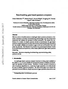
1.1 The structure and photophysics and holeburning [14] experiments showed, that both ground and excited state are spin triplets. The optical transition was determined to be 3 A - 3 E, which makes the ground state an orbitial singlet and the excited state an orbital douplet. However, the orbital doublet character can be neglected at room temperature, because very recently it was shown, that due to an averaging effect, which occurs at temperatures higher than 70 K, the excited state behaves like an effective orbital singlet [15, 16]. The current state of theory assumes that there are six electrons contributing to the energetic structure of the NV center [17]. Three electrons are provided by the carbon dangling bonds at the vacancy site, two electrons by the nitrogen atom and one electron is additionally caught, making the NV center negatively charged. There also exists a neutrally charged version of the NV center, the NV0 center, which has completely different properties and is not subject of this thesis [18]. Using off-resonant green (523 nm) laser light the system can be pumped into the excited state phonon sideband. Subsequent fast phonon relaxation brings the system to the lowest excited state. Spontaneous emission into the broad phonon band of the ground state leads to redshifted fluorescence (highest intensity between 650-800 nm). The high quantum fluorescence yield of this transition along with high photo stability allow single NV detection by standard confocal microscopy techniques. Actually, its extreme photo stability lead to the first commercially available single photon source1 . However, the full richness of the photophysics is only discovered by taking into account the triplet character of ground and excited state and the existence of a third electronic state (figure 1.2). Due to spin-spin-dipole interaction of the unpaired electron spins the ms = 0 spin state is split from the ms = ±1 states by 2.87 GHz in the electronic ground state. This interaction results in a strong quantization axis (the NV axis) for the electron spin. The optical transition 3 A - 3 E is spin conserving, because the quantization axis for the electron spin is the same in ground and excited state, the spin-orbit coupling in the excited state is very low at room temperature and the optical dipole operator does not mix spin states. The third electronic state is a metastable singlet lying energetically between ground and excited state. If the system is in the ms = ±1 states of the excited state, it has a high probability (about 50%) to relax radiationless into the A1 metastable singlet state instead into the ground state. Axial spin-orbit coupling permits this intersystem-crossing (ISC). Due to symmetry caused selection rules the transition of ms = 0 states from the excited state into the metastable state is forbidden, making the fluorescent transition the only decay channel for the ms = 0 state. Small non-axial spin-orbit coupling relaxes this prohibition, thus the ISC rate for the ms = 0 has a non-zero value, but nevertheless it is very small. Once the system has reached the longliving metastable state it is trapped there for 250 ns [19]. During this time, the system cannot be excited and cannot emit photons, therefore the average fluorescence intensity drops. Because mainly the ms = ±1 states relax into the metastable state, the average fluorescence contains information about the spin 1

Quantum Communications Victoria

9

Chapter 1 The Nitrogen-Vacancy center in diamond

excited state

ms +1 -1 0

ms= 0

ground state

metastable state

+1 -1

0

Figure 1.2: NV center energy level scheme at room temperature. The optical transistions are spin conserving. The alternative decay channel permits spin flips mainly from ms = ±1 into the ms = 0 state. This intersystem crossing leads to spin state dependent fluorescence and optical polarization into the ms = 0 state. state. Thus, the ms = 0 state can be considered as bright state and the ms = ±1 as dark states. The decay rates from the metastable state back in the groundstate are determined by symmetry and lead predominantly to population of the ms = 0 state. Thus, the second decay channel ends mainly in the ms = 0 state. Every optical run increases the probability of finding the system in the ms = 0 state, creating a non-Boltzmann and strongly polarized distribution of the spin states. Recent publications indicate that the alternative decay channel does not consist of one but two single metastable states [20]. However, for the purposes of this thesis it is totally sufficient to think of one metastable singlet state with a lifetime of about 250 ns. In summary, the electron spin state can be read out by recording the average fluorescence intensity and continuous laser excitation leads to spin polarization into the ms = 0 state. These two exceptional properties of the NV center, caused by symmetry and advantageous order of the energylevels, are the main reasons for the huge interest in this system and why it is considered as a promising candidate for solid state quantum computing at room temperature.

1.2 Experimental setup To detect single quantum emitters optically, two important requirements have to be fulfilled. First, the emitters have to show strong fluorescence and second, the density

10

1.2 Experimental setup

APD

of the emitters must be low enough. Both needs are easily met by diamonds with a NV density below 0.5 ppb. The experimental setup for single defect spectroscopy is basically a high resolution confocal microscope (figure 1.3), which operates at room temperature. A 532 nm cw laser (frequency-doubled Nd:YAG) is focused by an objective

diamond sample

rf amp

fiber

 647nm longpass

1 st dif

fr. or d

er

rf source

AOM

objective on piezo

switches mw source

lense

APD

20 m copper wire

mw amp

lense

glass wedge

electro magnet

time correlation

50 m pinhole

532 nm

pulse generator

Figure 1.3: Scheme of the experimental setup. and excites a small diffraction limited volume (below 1 µm3 ) in the diamond, wherefrom the fluorescence is collected. For pulsed experiments, the laser passes an acousto optical modulator (AOM). By applying RF at the AOM crystal a standing wave is formed and the laser light is diffracted by the resulting optical grating. Only the first diffraction order can pass the rest of the beam path, the others are blocked. Switching on and off the RF creates laser pulses with a rise time of about 10 ns. Passing the beam through a photonic fiber increases the quality of the light mode. The laser beam is guided into the objective by a glass wedge, which reflects about 5-10 %. The objective is mounted on a piezo scanner (range: 100 µm x 100 µm x 20 µm). If the objective is moved by the piezo, the focus in the diamond moves as well. The fluorescence is collected by the same objective to ensure a good overlap of excitation and detection volume. In order to increase the number of collected photons, an oil immersion objective is used (NA= 1.3). The high difference of the refractive indices of diamond (ndia = 2.4) and air (nair = 1) causes a small total internal reflection angle at the border. By using immersion oil (noil = 1.5) between diamond and objective, the angle is increased and more photons can leave the diamond. A lens focuses the fluorescence

11

Chapter 1 The Nitrogen-Vacancy center in diamond onto a small pinhole (50 µm diameter) to increase the signal to background ratio by blocking the light from other planes than the focal plane. Behind the pinhole, a 647 nm longpass cuts away reflected laser light and only fluorescence photons enter the last part of the detection channel, the Hanbury Brown and Twiss setup. This setup consists of a beamsplitter and two avalanche photo detectors (APD). By measuring the temporal correlation between two photon arrivals, one at each APD, the number of single quantum emitters can be determined. This measurement relies on the fact, that a single emitter cannot emit two photons at the same time. During its radiative relaxation from the excited to the ground state it cannot be reexcited, but the reexciation is necessary for a second photon. Thus, the probability for one photon at each APD at the same time is zero for a single quantum emitter. This correlation function is called the second order correlation of the light field g (2) (τ ) and the verification of a single emitter is valid for g (2) (0) < 0.5 (figure 1.4). The NV fluorescence saturates at about 350 µW excitation laser power and yields up to 250 kc/s at the detectors. This corresponds to an overall photon detection efficiency of 2% (radiative lifetime = 12 ns). Spin transitions can be tuned by applying a static magnetic field. For this purpose, an

b)

a)

45

1,0

y[]

g(2)(τ)

1,5

15

10 35

0,5

5

(2)

g (0) < 0.5 0,0

25

0

τ [ns]

300

35

45

x[]

Figure 1.4: a) Measurement of the second order correlation function g (2) (τ ) to verify single quantum emitters. b) 25 µm x 25 µm confocal scan. The bright spots are mainly single NV centers electro magnet, which can create fields up to 0.4 T, is placed behind the sampleholder on a moveable stage. The magnet can be shifted in 3 dimensions and rotated around 360◦ , thus it is possible to apply a static magnetic fields along arbitrary directions. A thin copper wire (20 µm diameter) spanned over the diamond permits the application of microwave (mw) and radiofrequency (rf) radiation for resonant electron and nuclear spin manipulations. The wire is soldered to the sampleholder, which is connected to various mw and rf sources and amplifiers. Pulse experiments with a sequence of laser, mw

12

1.3 Spin Hamiltonian and rf pulses are performed with a pulsegenerator, which gives TTL pulses to switches, which control the rf for the AOM and the mw and rf sources for spin manipulation.

1.3 Spin Hamiltonian Since this thesis is dedicated to spin physics, the NV ground state spin Hamiltonian is briefly introduced before the basic electron spin resonance experiments are discussed. The whole spin Hamiltonian can be expressed by electron and nuclear spin operators and numerical parameters only. There is no need for operators acting e.g. on the spatial coordinate of the electron. The spatial wavefunction is averaged and hidden in the different parameters of the Hamiltonian. These parameters can be determined by magnetic resonance techniques. In the electronic ground state the spin Hamiltonian can be divided into the following contributions (energetically ordered): H = HZF + HEZ + HHF + HN Q + HN Z

(1.1)

The largest energy scale is given by the dipole-dipole-interaction of the unpaired electrons. The degeneracy of the ms = 0 and ms = ±1 spin levels is lifted by 2.87 GHz zero-field splitting, with the corresponding Hamiltonian ~ DS ~ HZF = S

(1.2)

~ is the electron spin vector operator and D is the zero-field splitting tensor, which can S be expressed by two independent parameters D and E. HZF = D · Sz2 + E · (Sx2 − Sy2 )

(1.3)

D is 2.87 GHz in the ground state. E describes the deviation from axial C3ν symmetry. E = 0 means perfect symmetry, whereas a non-zero value can be caused by strain in the crystal or by an electric field. In CVD bulk diamonds E is usually negligible. The second largest contribution is the electron Zeeman term, which lifts the degeneracy of the ms = ±1 states. The static magnetic field is aligned along the z-axis (NV-axis) in most of the experiments reported in this thesis HEZ = ge µB Bz Sz .

(1.4)

µB is the Bohr magneton and the electron g-factor ge is equal to the free electron case (ge = 2.0023). The magnetic dipole moment of the NV can also interact with nearby nuclear spins. This hyperfine interaction has an isotropic Fermi contact and an anisotropic dipole-dipole contribution. X ~ I~i + ST ~ I~i ) HHF = (aiso,i · S (1.5) i

13

Chapter 1 The Nitrogen-Vacancy center in diamond The isotropic parameter aiso,i is proportional to the probability density of the electron spin at the nucleus i. This is a purely quantum mechanical effect, which arises from symmetry constraints to the complete wavefunction (spatial and spin part). The anisotropic interaction is characterized by the symmetric and traceless tensor T. Its origin is the classically understandable interaction of two magnetic dipoles. T can be in principle calculated by averaging the full magnetic dipole-dipole Hamiltonian HDD over the spatial coordinates,    X µ0 µB µn ge gn,i  ~ · I~i − 3 S ~ · r~i I~i · r~i , S (1.6) HDD = 3 4πr i where µ0 is the vacuum permeability, µn is the nuclear magneton and gn,i the g-factor of nucleus i. The vector ri links the electron with the proper nuclear dipole. Because of the strongly localized electron wavefunction the dipole-dipole contribution dominates the interaction with nuclear spins which are more than three bond lengths separated from the NV center. The first nuclear spin, which comes into mind for hyperfine interaction, is the nitrogen nucleus as a component of the NV center. It exists in two isotopes, 14 N (I= 1) and 15 N (I= 1/2), whereas 15 N has a very low natural abundance (= 0.1 %). For the case of 14 N (I= 1) there is an additional term in the spin Hamiltonian, the quadrupole coupling.   1~2 2 (1.7) HQN = P Iz, N − IN 3 It leads to a zero-field splitting P of the nuclear spin levels similar to the electron spin, but a factor 600 lower. However, there is also another species of nuclear spins in the diamond, the 13 C isotope (I= 1/2), which has a natural abundance of 1.1 %. Because of the strong distance dependence of both Fermi contact and dipole-dipole coupling, one might expect the hyperfine coupling to the nitrogen nuclear spin to be much larger than to the 13 C nucleus, but this is not necessarily the case. It turns out that the electron spin density at the nitrogen atom is pretty low in the groundstate and that the electron is mostly at the vacancy site. This leads to very strong hyperfine interaction (up to 130 MHz) of the NV electron spin with 13 C atoms close to the vacancy site. The interaction with the nitrogen nucleus is discussed in more detail in chapter 2. The static magnetic field couples also to nuclear spins, which gives the last term considered, the nuclear Zeeman energy HN Z = ge µn Bz Iz .

(1.8)

The nuclear Zeeman splitting is on the order of 0-400 kHz for the presented experiments. Writing down a Hamiltonian means drawing a line between the system and the environment and neglecting terms in a solid state system is unavoidable. In this case inter nuclear coupling is neglected, which leads e.g. to dephasing of the NV electron spin and can be described by phenomenological decoherence times.

14

1.4 Optically detected magnetic resonance (ODMR)

1.4 Optically detected magnetic resonance (ODMR) As the ground state of the NV center is a spin triplet it can be investigated by means of magnetic resonance. Electron spin resonance (ESR) measures the magnetization, i.e. the population difference of spin levels. Usually, in order to achieve detectable population differences high magnetic fields or very low temperatures are necessary, because in thermal equilibrium the spin state populations are determined by the Boltzmann distribution and unequal populations need µB gB > kT . However, this is not the case for the NV center. Continuous laser excitation leads to strong polarization into the ms = 0 spin state. Due to very long longitudinal relaxation times even at room temperature (5 - 10 ms), there is plenty of time to perform magnetic resonance experiments before the Boltzmann distribution is recovered. Because of the strong spin state dependence of the fluorescence intensity it is possible to perform optically detected magnetic resonance (ODMR). Due to single defect laser excitation and fluorescence detection with a confocal microscope, ODMR at the single level is possible.

a)

b) 48000

IPl [a.u.]

IPl [a.u.]

48000 44000

44000 40000 2700

2800

2900

MW [MHz]

3000

2700

2800

2900

MW [MHz]

3000

Figure 1.5: a) Optically detected magnetic resonance of the NV center at zero magnetic field. At the frequency of the zero-field splitting of 2870 MHz, population is transfered from the bright into the dark state. This causes a drop in the fluorescence. b) A static magnetic field parallel to the NV axis lifts the degeneracy of the ms = ±1 states. Continuous laser excitation (532 nm) polarizes the electron into its bright state. By applying simultaneously mw radiation, the ESR signal can be detected as a dip in the fluorescence. Hence, the fluorescence intensity over the applied microwave frequency is observed. If the mw is in resonance with the spin transition, population is transferred from the bright state to the dark state. In figure 1.5 a), a NV ODMR spectrum is shown. At the frequency of the zero-field-splitting a dip in the fluorescence is observed. In a static magnetic field, these lines are split by the Zeeman energy (figure 1.5 b). If the

15

Chapter 1 The Nitrogen-Vacancy center in diamond field is aligned along the NV axis the splitting is increasing linearly with the magnetic field amplitude. |2870 MHz − ν0↔±1 | = 2.8 MHz/Gauss · B

(1.9)

The two spectra are both laser and mw power broadened. By reducing the power, the hyperfine structure becomes visible. Figure 1.6 shows the spectra of two NVs. In both cases a magnetic field along the NV axis is applied and only the electron spin ms =0 ms =-1 transition is shown. The two NVs have different nitrogen isotopes, one consists of a 14 N, the other of a 15 N. The 14 N is a nuclear spin I = 1 system and the spectrum shows

a)

b) 15000

IPl [a.u.]

IPl [a.u.]

45000

14000

40000

2755

2760

MW [MHz]

2765

2795

2800

MW [MHz]

2805

Figure 1.6: Hyperfine resolved ODMR spectra of two NVs with different nitogen isotopes. Only the electron spin ms = 0 - ms = -1 transition is shown. a) 14 N, I= 1. b) 15 N, I= 1/2

three lines equally separated by 2.15 MHz. These three lines correspond to three nuclear spin quantum numbers (mI = -1, 0, +1), which are conserved by the mw transition. The 14 N nuclear spin is topic of a more detailed investigation in chapter 2. The 15 N has a nuclear spin I = 1/2. Thus, there are two allowed mw transitions (split by 3 MHz) for the two possible components of the nuclear spin along the NV axis (mI = -1/2, +1/2). The splittings are due to hyperfine interaction in the ms = -1 state. In ms = 0 the electron spin does not couple to the dipole field from the nuclear spin and the nuclear spin states are only split by the nuclear Zeeman energy, which is negligible for low magnetic fields. Continuous wave ODMR spectroscopy provides some information about the difference of energy levels of the NV electron spin but to observe coherent spin dynamics pulse experiments are necessary.

16

1.5 Determination of the spin state

1.5 Determination of the spin state The three parts of a spin pulse experiment are: initialization, manipulation and read out. The initialization is done by a short green laser pulse. Before showing particular spin experiments, the readout process is discussed. As mentioned in section 1.1, the fluorescence depends strongly on the electron spin state, i.e. the shape of a fluorescence pulse depends on the spin state as well. In figure 1.7 two NV fluorescence pulses are shown. In figure 1.7 a) the initial spin state is ms = 0 and

b) 60

# of fluorescence photons

# of fluorescence photons

a) 60

30

0

0

1000

2000

ns

3000

40

20

0

0

1000

ns

2000

3000

Figure 1.7: NV fluorescence during a 3 µs excitation laser pulse (532 nm). The time bining is 1 ns and to get the average fluorescence the measurement is repeated 280,000 times, i.e. every bin is measured 280 µs. The red line is calculated with classical rate equations for a five level modell (figure 1.8). The rates are fitted to the data. a) Initial spin state ms = 0. Starting polarized in the bright state, the fluorescence drops, because a small steady-state population is build up in the meta stable state b) Initial spin state ms = -1. The high ISC for the ms = -1 state brings the system into the longliving metastable state and during its lifetime the system does not emit photons. The initial decay is determined by the ISC rate for the ms = -1 state, whereas the recovery rate represents the lifetime of the metastable state. thus the fluorescence intensity is high at the beginning, because the system undergoes many optical cycles. In the steady state the fluorescence is a little bit lower, because the metastable state gets slightly populated. This is caused by the small but non-zero ISC rate for the ms = 0 in the excited state. In figure 1.7 b), the dark ms = -1 state is populated initially and the fluorescence drops at the beginning, because of the radiationless ISC from ms = -1 in the excited state. This leads to lower fluorescence. Whereas the ISC rate into the metastable state is responsible for the initial fluorescence lowering (in both cases), the ISC rate into the ground state determines the time needed to polarize the spin into its bright state. The characteristics of these pulses are well reproduced by a

17

Chapter 1 The Nitrogen-Vacancy center in diamond simple five level picture (figure 1.8 a)). For simplicity, only one dark state in ground and excited state is considered. Assuming that the optical coherences decay very fast, it is easy to set up a classical rate equation system for the five populations (similar to [17]). The rates are fitted to experimental data and the good agreement in both cases indicates that the polarization mechanism via the metastable state is well understood.

a)

b)

excited state metastable state

signal / noise

40

max  350 ns

30

20

10

ground state

0

0

1000

tp [ns]

2000

3000

Figure 1.8: a) The five level modell used to reproduce the spin depending fluorescence. The arrows show which rates are taken into account and the thickness indicates the strength of the rate (the thicker the larger). b) Signal to noise as a fuction of tp calculated for the two pulses in figure 1.7 The fluorescence pulses in figure 1.7 differ only during the first 500 ns. Afterwards there is no difference in the fluorescence left. Thus, by comparing the number of photons at the beginning of these two pulses, the spin state can be distinguished. To do this more p quantitatively the spin state signal ffref is introduced. fp is the number of photons up to a time tp , whereas fref is the number of photons at the end of the pulse. fp (tp ) =

tp X 0

# of photons(t)

fref (tref ) =

end X

# of photons(t)

(1.10)

end of pulse−tref

The division by fref is not essential but it normalizes the signal and also cancels fluctuations in the laser intensity. The tref time is not crucial for the signal to noise ratio, because at the end of the pulse the spin is polarized and the steady state is reached. tref is usually chosen to be 1 µs. In contrast, the choice of tp is more crucial for the signal to noise ratio. Extending tp by ∆tp increases the number of photons, which contain spin state information by ∆nsignal , but also the number of photons without information by ∆nnoise . Whereas the ∆nsignal

18

1.6 Spin Dynamics decreases exponentially with ∆tp , ∆nnoise is nearly contant. √ The photons obey the poissonian distribution and therefore give rise to a noise ∝ ntotal . Apparently, there must be a optimal value for tp with respect to the signal to noise ratio. The exact value is laser power depending and is about 350 ns for the case of optical saturation. However, for a particular experimental situation this value is calculated by dividing the number of spin-state-information containing photons by the squareroot of the total number of collected photons as a function of tp . For this purpose it is convenient to take the pulses, which belong to the most different spin states, bright and dark state, and consider the difference fp,bright − fp,dark as signal. number of signal photons fp,bright − fp,dark signal =√ =p noise total number of photons fp,bright + fp,dark

(1.11)

Figure 1.8 b) shows the signal to noise ratio as function of tp for the two pulses in figure 1.7. Note that the maximum is relatively broad. How the signal to noise ratio can be significantly increased by using the hyperfine coupling to the nitrogen nuclear spin is presented in chapter 2.

1.6 Spin Dynamics Coherence properties of spins can be observed by pulsed ESR experiments. They provide information about the coupling of the electron spin to its environment. Performing pulsed ODMR on the NV center is straightforward. The experiment starts always with short green laser pulse (= 3 µs) to initialize the electron spin in the ms = 0 state. Depending on the particular situation, a certain sequence of mw/rf pulses and free evolution time is applied for the desired spin manipulation. At the end a short laser pulse reads out the spin state and reinitializes it for the next run. The spin polarization is determined by comparing the average fluorescence at the beginning (first 350 ns) and the end of this final laser pulse, as described in section 1.5. As the averaged fluorescence is needed the whole sequence is repeated many times, e.g. 100.000 times. The fundamental ESR experiments are spin 1/2 i.e. two level dynamics. Applying a small magnetic field splits the ms = -1 state from the ms = +1 state, making e.g. the ms = 0 - ms = -1 transition an effective two level system. To get a more intuitive understanding of the dynamics it may be helpful to point out that in quantum mechanics the state of a two level system can be visualized on the Bloch sphere. Any point on the sphere represents a particular state of the system. The north pole corresponds to the bright ms = 0 state, the south to the dark ms = -1 and every other point to a particular supersposition state. The most basic experiment to observe coherent spin dynamics is the Rabi oscillation (figure 1.9) [21]. After the initialization laser pulse a resonant mw pulse drives the spin transition, e.g. the population is transferred coherently. On the Bloch sphere this means rotation around an axis in the x-y-plane. In order to record the Rabi oscillations the

19

Chapter 1 The Nitrogen-Vacancy center in diamond spin state after the mw pulse is read out and the duration τ of the mw pulse is steadily increased. After a certain τ the electron spin is brought into a superposition state with identical amplitudes (|ms i): |0i + |−1i (reaching the equator on the Bloch sphere). The corresponding mw pulse is called ‘π/2 pulse’. After twice this time (‘π pulse’) the population is fully transferred in the ms = -1 state, thus the fluorescence is the lowest. The oscillation frequency Ω depends linearly on the amplitude of the driving field (Ω ∝ B1 ). At the setup introduced in section 1.2, Rabi frequencies up to 100 MHz are possible.

a)

z

b)

ms= 0

y

x

IPl [a.u.]

1,0

0,9

0,8

ms= -1

0,00

0,05

0,10

0,15

τ [ns]

Figure 1.9: a) The state of a quantum mechanical two level system can be represented on a sphere (Bloch sphere). The dashed line shows the path, which takes the state vector during a half Rabi oscillation around the x-axis. b) Electron spin Rabi oscillation. The spin starts in the bright ms = 0 state and is transfered coherently into the dark ms = -1 state and back. To probe the coherence properties of the NV electron spin, sequences with a free evolution part are necessary. A requirement for long coherence times is a small lateral relaxation rate of the spin. In a soild phonons can interact with the spin system by spin-orbit coupling. For the NV center this coupling is very weak and additionally the density of phonons in diamond even at room temperature is very low. This permits very long spin relaxation time (≈ 10 ms). A sensitive way to probe the magnetic environment of the electron spin is the free induction decay (FID). The electron spin is polarized and a subsequent π/2 pulse creates a superposition spin state. After a free evolution time τ the superposition state is transformed back into a population difference by a second π/2 pulse. The FID is recorded by extending the free evolution time τ . If the first π/2 pulse is not in resonance with the mw transition but slightly detuned, the phase of the superposition state oscillates during the free evolution. The oscillation frequency is equal to the detuning (ωmw − ωesr ). As

20

1.6 Spin Dynamics the second π/2 pulse maps coherence into population, an oscillation in the phase leads to oscillation in the population (also called Ramsey-fringes). The signal decays with increasing free evolution time τ . This FID decay time is called T∗2 and the origin of this loss of coherence are changes in the magnetic environment of the electron spin. Nuclear and electron spins far away from the NV center act as a spin bath, thus the magnetic field at the NV center varies in time. The pulse sequence is repeated 100.000 times and in every run the nuclear spin configuration is slightly different. As the superposition state acts as a sensitive magnetometer, it picks up a different phase during the free evolution in every run. This causes the decay of the oscillation. The line width in the FFT of the FID corresponds to the inhomogeneously broadened ESR transition. Recently it was shown, that the main decoherence source in pure type IIa diamonds is the spin bath formed by 13 C atoms [22]. In bulk diamonds with a natural abundance of 13 C, T∗2 is of the order 5-10 µs. However, in 13 C purified diamonds (99.998 % 12 C) T∗2 times around 60 µs (figure 1.10) are measured. The corresponding line width is 6 kHz.

a)



π 2

b)

π

π

2

2

π



π 2

1,05

IPl [a.u.]

IPl [a.u.]

1,0



0,9

1,00

0,8 0

50

100

τ [µs]

150

200

0,95

0

1

2

2τ [ms]

3

Figure 1.10: Coherence measurements of the NV eletron spin in an ultra pure diamond (99.998% 12 C). a) Free induction decay, T∗2 ≈ 60 µs). b) Spin Echo, T2 ≈ 2.6 ms

A single spin, which experiences a slightly different magnetic field from shot to shot, is similar to a spin ensemble, where every spin has its own magnetic environment. This makes the well known ensemble ESR/NMR toolbox available, e.g. spin echoes. The basic spin echo was already invented in 1950 by Otto Hahn and was a milestone in the development of NMR [23]. The pulse sequence is π/2 - τ - π - τ - π/2. In the first free evolution time the spin picks up a certain phase φ. The π pulse in the middle of the sequence induces a phase change φ 7→ −φ. In the second free evolution time the same

21

Chapter 1 The Nitrogen-Vacancy center in diamond phase φ is picked up again and the opposite phases cancel each other. This Hahn echo refocuses slow varying magnetic fields compared to 2 τ . The decay time of the Hahn echo is called T2 or just decoherence time. In the above mentioned ultrapure crystal the NV electron spin reaches T2 times up to 2.6 ms (figure 1.10 b)).

1.7 Basic aspects of quantum information processing (QIP) with the NV center In the 1980‘s the idea came up to use the laws of quantum mechanics for information processing purposes. Based on pioneering considerations of R. Feynman and D. Deutsch [24, 25, 26], P. Shor showed one decade later in 1992, that a device, which uses quantum mechanical properties like superposition, can factorize large numbers exponentially faster than a classical computer [27]. In the following years more and more examples for outperforming quantum algorithms were found, e.g. Grover‘s algorithm for searching an unsorted database [28]. To get the basic idea and advantage of quantum computing (QC), one should remind classical computing. A classical memory consists of a certain number of bits. One bit is either in the 0 (=|0i) or the 1 (=|1i) state at the beginning. Performing an algorithm changes the values of the bits in some desired way and the state of the memory at the end is the result. At every moment of the calculation the bits have one of the two possible values. If instead the bits obey the laws of quantum mechanics, superpositions of these values would be allowed. Additionally to 1 and 0 states, the quantum bit (qubit) can be in any superposition state α |0i + β |1i (α,β complex numbers with |α|2 + |β|2 =1) during the computational phase. Both values, connected by a certain phase, can run through the algorithm simultaneously. This phenomenon is called ‘quantum parallelism’ and is the origin of the outperforming computational power of the quantum algorithms. Several different computation models for QIP have been developed in the last 20 years [29, 1, 30]. In the quantum circuit model quantum algorithms consist of a series of unitary operations (called gates) on a prior initialized set of qubits. Like in the classical case the result is the output state. It has been shown, that a universal quantum computer, which can perform any quantum algorithm, needs only to be able to perform two kinds of gates [1]. The first gate is the one-qubit-rotation (referred to as local operation) i.e. any superposition α |0i + β |1i can be transfered into an arbitrary δ |0i + γ |1i state (δ,γ complex numbers, with |δ|2 + |γ|2 =1). In the picture of the Bloch sphere this means that every point of the sphere has to be reachable. The second important gate is the CNOT. This two qubit gate flips the target qubit depending on the state of the control qubit. The CNOT can be represent in the product

22

1.7 Basic aspects of quantum information processing (QIP) with the NV center basis of two qubits (|00i,|01i,|10i,|11i) by the matrix   1 0 0 0  0 1 0 0     0 0 0 1  0 0 1 0

(1.12)

The importance of the CNOT is caused by its entangling action on two appropriately prepared qubits, e.g. two qubits, initially prepared in the productstate ((|0i + |1i) ⊗ |0i) (the first/second qubit is the control/target qubit), get entangled by applying the CNOT ( → |00i + |11i). An entangled state cannot be expressed as a product of the two single qubit states [31, 32]. The correlation of entangled qubits are non-classical and thus entanglement is also an origin of the power of QC. Actually two other gates can be chosen as universal gates, but at least one two qubit gate is necessary. In 2000 D. DiVincenzo summarized the five most fundamental requirements on a physical implantations of a quantum computer [33]: • A scalable physical system with well characterized qubits • The ability to initialize the state of the qubits • Long relevant decoherence times • A universal set of quantum gates • A qubit-specific measurement capability Until today the physical implementation of a powerful quantum computer is an unsolved problem, but there has been a lot of progress and proof-of-principle experiments in the last 15 years (e.g. [2, 3, 4, 34, 35, 36, 37, 38]). As a qubit is simply a two dimensional quantum mechanical system, there is no clear best hardware for QC. Indeed, the two universal gates were realized with a number of different types of qubits like spin-qubit, photonic-qubit or superconducting-qubit. Among these different systems is the NV center in diamond. The qubit can be a single electron spin transition in the groundstate, e.g. ms = 0 ↔ ms = -1. If the system provides three states, like the NV electron spin, it is referred to as qutrit. The initialization is done very efficiently and fast by a short laser pulse. The single qubit rotations correspond basically to Rabi oscillations and the realization of a CNOT-gate with a 13 C nuclear spin as second qubit was already shown in 2004 [5]. The readout process is performed by measuring the average fluorescence intensity. This is only sensitive to the electron spin state, but nevertheless by mapping the nuclear spin onto the electron spin the nuclear spin state can be readout. Due to the fact, that 12 C has no nuclear spin diamond provides a almost spin free environment and is the perfect host for a spin qubits associated with impurities, as it permits very long coherence times. The scalability of a NV center based

23

Chapter 1 The Nitrogen-Vacancy center in diamond quantum computer is addressed in section 3.1. Because the NV center is a solid state system and the spin experiments are performed at room temperature, it is deemed to be a promising candidate for a realistic QC.

1.8 Conclusion In this chapter, the NV center in diamond has been introduced. This defect center is an electron spin triplet system in the ground state, which spin state can be readout and initialized by optical means. The experimental setup is basically a homebuild confocal microscope, which allows single center detection and thus optically detected magnetic resonance at the single spin level is possible. Static magnetic fields are used to shift the ESR frequencies and spin manipulations by mircowave radiation, e.g. Rabi oscillations, demonstrate a high degree of control over the electron spin. The coherence times of the NV electron spin, investigated by free induction decay and Hahn spin echo, are the longest for an electron spin in a solid state system at room temperature. Summarizing, the NV electron spin fulfills the DiVincenzo criteria on a physical realisation of a qubit, which can be used for quantum computation purposes [33]. Up to now NV quantum registers have been extended by hyperfine coupling to nearby 13 C nuclear spins [7]. In the chapter 2, the coupling of the NV electron spin to the 14 N nuclear spin is exploited for obtaining an additional nuclear spin qutrit and for enhanced optical spin readout. In chapter 3, the scalability is discussed and the coupling of two nearby NV centers, artificially engineered by ion implantation, demonstrates that the number of NV qubits is in principle not limited.

24

Chapter 2 Coherent coupling to the 14N nuclear spin As nitrogen is an essential part of the NV center, the NV electron spin experiences always the presence of a second spin: the nitrogen nuclear spin. This chapter is dedicated to the coupling of these two spins. The investigations are motivated by several reasons. First of all, the general understanding and characterization of the NV center can be improved as the coupling is an intrinsic part of the NV. A second motivation is the aim to increase the number of controllable qubits. In the first chapter it is shown that the NV electron spin can be used as qutrit and previous publications demonstrated the coherent control over nearby 13 C nuclear spins [5, 7], whereas the applicability of the nitrogen nuclear spin for quantum computation purposes has not yet been investigated. Nuclear spin qubits have the advantage of very long coherence times due to their weak interaction with the environment. Another reason for the interest in the 14 N nuclear spin is the possiblilty of using it for enhancing the optical electron spin readout fidelity. Actually, the major result of this chapter is the possibility of spin state determination by a single run of the readout sequence.

2.1 Spectroscopy The hyperfine interaction of the NV electron spin with the nitrogen nucleus is investigated. In order to get a precise description of the coupling the energy level structure is revealed in detail by different spectroscopy techniques. As mentioned in section 1.3, the nitrogen nuclear spin is a spin triplett like the NV electron spin. Quadrupole interaction lifts the degenerary of the nuclear spin levels mI = 0 and mI = ±1. If the electron spin is in the ms = ±1 states, its dipole field results in a hyperfine interaction between electron and nuclear spin. The underlying Hamiltonian is given by:   1~2 2 HN = P Iz, N − IN + Ak Sz Iz, N + A⊥ (Sx Ix, N + Sy Iy, N ) + gN µN Bz Iz 3

(2.1)

25

Chapter 2 Coherent coupling to the

14

N nuclear spin

where P descibes the quadrupole interaction. Its literature value of ≈ 5 MHz has been determined by ensemble measurements [39, 40]. The hyperfine interaction in the ms = ±1 states shifts the mI = ±1 states by ± Ak . Because of the large zero-field splitting of the electron spin, the hyperfine interaction perpendicular to the NV axis can be neglected when considering the energy level structure (secular approximation). The last term of the Hamiltonian is the nuclear Zeeman energy which is on the order of a few hundreds kHz in the presented experiments. The resulting level structure is depicted in figure 2.1 a). The parallel hyperfine parameter Ak can be obtained directly from the ESR spectrum. Figure 2.1 b) shows a spectrum of one NV electron transition (|0i ↔ |−1i), where the three lines correspond to the three nuclear spin states. The ESR transitions are nuclear spin state conserving as the quantization axis of the nuclear spin is not depending on the electron spin state. Its quantization axis is given by the quadrupole tensor and neither the used static magnetic fields nor the dipole field of the NV electron spin have a component perpendicular to this axis, which is on the same order of magnitude. According to Hamiltonian HN the ESR lines are shifted by mI · Ak . From spectrum 2.1 b) a value of ≈ 2.2 MHz can be obtained. The width of the lines in the ESR spectrum are given by the T∗2 coherence time of the electron spin and this limits the accuracy of the determination of Ak to the order of 100 kHz. As the quadrupole interaction P does not depend on the electron spin state, it does not influence the ESR transitions and thus P cannot be obtained from the ESR spectrum. In order to show a coherent control over the nitrogen nuclear spin and its usability as qutrit, it is necessary to determine the parameters P and Ak more precisely. As the actual width of the nuclear transition is given by the long T∗2, N coherence time of the nuclear spin, the parameters should be determinable at least one order of magnitude more precisely. Nuclear magnetic resonance on a single nucleus can be performed by using the NV electron spin as readout device. In general, techniques, which measure nuclear spin transitions by probing electron spin transitions are called Electron Nuclear Double Resonance (ENDOR). In ensemble magnetic resonance experiments, ENDOR is usually used to take advantage of the higher polarization and energy regime of the electron spins and this results in enhanced sensitivity [41]. ENDOR experiments on the NV center have been shown for 13 C nuclear spins [5, 7]. A typical pulse sequence for measurement of a nuclear spin spectrum by ENDOR is illustrated in figure 2.2 a). The electron spin is polarized by a short laser pulse. Thus, the electron spin state is ms = 0, whereas the nuclear spin is in a incoherent mixture. A nuclear spin state selective mw π pulse populates one nuclear spin sublevel in ms = -1 e.g. the mI = +1 state (see blue arrow in 2.1 a)). This selectivity is achieved by driving the transitions at Rabi frequencies, which are low compared to the detuning to next ESR transistion e.g. Rabi frequencies of 500 kHz if the detuning is 2 MHz. A subsequent rf pulse is applied to drive the nuclear spin transition (|ms , mI i; |−1, +1i ↔ |−1, 0i). To measure the effect of the rf pulse, the nuclear spin state (in ms = -1) is mapped back onto the electron spin by a second

26

2.1 Spectroscopy

a)

b)

mI ms= +1

0 -1 +1

P +- A 60000

mI

ms= -1

0 +1 -1

P +- A

IPl [a.u.]

-1 0 +1 58000

56000

ms= 0

0 -1, +1

2840

P

2850

2860

2870

MW [MHz]

Figure 2.1: a) Energy level scheme: The nitrogen nuclear spin couples to the NV electron spin. Colored arrows represent the ESR lines of the spectrum on the right. Nuclear Zeeman splitting is neclected. b) Hyperfine resolved ESR spectrum (closeup of ms = 0 ↔ ms = -1 transition)

27

Chapter 2 Coherent coupling to the

14

N nuclear spin

nuclear spin selective mw π pulse. If the rf pulse transfers some population from the mI = +1 state into the mI = 0 state, the subsequent mw pulse brings back less population into the ms = 0 state, which is readout by a final readout laser pulse. The spectrum is obtained by repeating this sequence while sweeping the rf frequence. The resonance of the rf with the nuclear spin transition, results in a dip in the fluorescence (figure 2.2 b)). The resolution is improved when using weaker rf pulses, as the nuclear Rabi frequency is reduced and hence small detunings have more impact.

b)

a) laser electron nuclear

π

π π

t

IPl [a.u.]

174000

172000

170000 2,7

2,8

2,9

3,0

3,1

3,2

RF [MHz]

Figure 2.2: a) ENDOR pulse sequence: The mw pulse is nuclear spin state selective and creates a nuclear spin polarization inside a certain electron spin subspace. After the rf pulse a subsequent mw pulses maps the effect of the rf pulse on the electron spin. An ENDOR spectrum is recorded by repeating the sequence while sweeping the frequency of the rf pulse. b) Measured ENDOR spectrum at low magnetic field. The detected transition is |−1, +1i ↔ |−1, 0i With the same pulse sequence it is also possible to detect nuclear transitions within the ms = 0 state, e.g. the spectrum shown in figure 2.3. This spectrum is recorded at a magnetic field of 500 Gauss, which splits the mI = ±1 levels by about 360 kHz. Note that this splitting is large compared to the nuclear rabi frequencies (of the order of 50 kHz) used here, hence the mI = 0 ↔ mI = ±1 transitions are distinguishable. By taking ENDOR spectra of the different transitions and at different magnetic field amplitudes, the parameters of the Hamiltonian HN , P and Ak can be obtained. These measuments have been performed for 3 NV centers in two different crystals1 . P = 4.945 ± 0.01 MHz Ak = 2.166 ± 0.01 MHz 1

(2.2) (2.3)

The experiments have been carried out in a 12 C-enriched (99.7 %) type IIa high-pressure high temperature diamond and in type IIa CVD diamond sample with natural abundance of 12 C.

28

IPl [a.u.]

2.2 Nuclear spin polarization due to spin dynamics in the excited state

43000

42000 4,6

4,8

RF [MHz]

5,0

Figure 2.3: ENDOR spectrum of the |0, +1i ↔ |0, 0i transition. The corresponding pulse sequence is the same as in figure 2.2 b). A single mesurement has narrower lines but the position varies slightly from center to center.

2.2 Nuclear spin polarization due to spin dynamics in the excited state The 14 N nuclear spin is polarized by optical excitation, when a magnetic field of about 500 Gauss is applied parallel to the NV axis. The polarization is observable in the ESR spectrum (figure 2.4). Instead of three lines split by 2.15 MHz, only one line is visible. The underlying mechanism is the same as recently reported for the 15 N nuclear spin [42]. It is based on spin dynamics in the excited state. As already mentioned in section 1.1, at room temperature the excited state can be considered as a spin triplett with a zero-field splitting of 1.4 GHz [43]. The orientation of the zero-field tensor as well as the electron spin g factor are the same as in the ground state. The corresponding spin Hamiltonian is:   1~2 2 2 2 2 ~ Aex I~ (2.4) Hex = Dex · Sz + Eex · (Sx − Sy ) + ge µB Bz Sz + Pex Iz, N − IN + S 3 At a magnetic field ampiltude of 500 Gauss (field is applied parallel to the NV axis), the Zeeman energy is as large as the zero field splitting and the ms = -1 state and the ms = 0 state cross each other (figure 2.5). Without hyperfine interaction the six states |−1, −1i,|−1, 0i,|−1, +1i,|0, −1i,|0, 0i,|0, +1i are degenerate. Therefore, small perturbations of the symmetry, e.g. contributions to the Hamiltonian ∝ Sx Ix determine

29

Chapter 2 Coherent coupling to the

14

N nuclear spin

IPl [a.u.]

76000

74000

72000

1415

1420

1425

MW [MHz]

1430

1435

Figure 2.4: ESR spectrum of the ms = -1 transition at 500 Gauss. Due to nuclear spin polarization only one hyperfine line (mI = +1) remains visible. the eigenstates, which results in a level anticrossing (LAC). Such a perturbation is perpendicular hyperfine interaction. The hyperfine splitting of 14 N in the excited state is known to be about 45 MHz, thus 20 times larger than in the groundstate [44]. This is due to a shift of the electron wavefunction towards the nitrogen nucleus in the excited state [45]. Assuming the interaction to be isotropic, the hyperfine part of the Hamiltonian is simplified. ~ Aex I~ = Aex S ~ · I~ S (2.5) The effect of the perpendicular component of the hyperfine interaction can be understood easily by rewriting this part: 1 Aex (Sx Ix + Sy Iy ) = Aex (S+ I− + S− I+ ) 2

(2.6)

where S± , I± are the usual ladder spin operators. Hence, the hyperfine interaction induces flip-flop proceses between the electron and the nitrogen nuclear spin. An impression of the characteristics of the flip-flop processes can be obtained by a closer look on the eigenstates of excited state spin Hamiltonian Hex . The perpendicular hyperfine interaction leads to new eigenstates, which can be expressed as superpositions of the high field states |−1, −1i, |−1, 0i, |0, 0i, |0, −1i (the states corrresponding to ms = +1 are omitted for simplicity): |+i1 = α |0, −1i + β |−1, 0i |−i1 = β |0, −1i − α |−1, 0i |+i2 = γ |0, 0i + δ |−1, +1i |−i2 = δ |0, 0i − γ |−1, +1i

30

(2.7) (2.8) (2.9) (2.10)

2.2 Nuclear spin polarization due to spin dynamics in the excited state where α, β, γ, δ are comlex numbers with |α|2 +|β|2 = 1 and |γ|2 +|δ|2 = 1. The |−1, −1i and the |0, +1i state are not affected by perpendicular hyperfine interaction and remain eigenstates, as no flip-flop process are possible (see inset in figure 2.5). The coefficients α,β,γ,δ depend on the magnetic field. In the √ high field limit α, γ → 1 and β, δ → 0, whereas at the LAC all coefficients are 1/ 2. If the system is pumped to the excited state from spin state |0, −1i, it is not in an eigenstate but in a superposition of the new eigenstates. The phase of this superposition precesses and after a whole oscillation the probability of finding the system in |−1, 0i is 4 |α|2 |β|2 . This corresponds to a flip-flop process. As the precession frequency is at least the perpendicular hyperfine interaction (≈ 45 MHz) and thus on the same order as the excited state decay rate, the coherent evolution in the excited state can be approximated by a classical flip-flop rate. It is valid to assume that the probability for a flip-flop process per cycle through the excited state is half the amplitude for the flipped state (4 |α|2 |β|2 / 2 = 2 |α|2 |β|2 ). Thus, the rates changes as a fuction of the magnetic field proportional to |α|2 |β|2 . Figure 2.6 shows the |α|2 |β|2 (red curve) and |γ|2 |δ|2 (black curve) as a function of the magnetic field. The two Lorentzians have maxima around 500 Gauss and are slightly shifted against each other.

ms

ES

+ -1

|-1,-1〉

0

E

|0,+1〉

GS

α|0,0〉 ± β|-1,+1〉 γ|-1,0〉 ± δ|0,-1〉

+ -1

0

450 0

500 1000

500

magnetic field [Gauss]

550

magnetic field [Gauss]

Figure 2.5: Ground and excited state energy level structure of the NV electron spin depending on the amplitude of a static magnetic field applied parallel to the NV axis. Around 500 Gauss a level anticrossing (LAC) occurs in the excited state. The closeup shows the hyperfine levels near the LAC. Two eigenstates are unaffected by the LAC (black curves, |−1, −1i and |0, +1i), whereas the other levels are mixed. Hence, in addition to the fluorescent decay and the ISC, two different flip-flop processes

31

Chapter 2 Coherent coupling to the

14

N nuclear spin

are possible in the excited state: |−1, 0i ↔ |0, −1i |−1, +1i ↔ |0, 0i

(2.11) (2.12)

This additional spin dynamic has a strong impact on the steady state nuclear spin distribution under continuous optical excitation. The electron spin is polarized by the optical excitation and thus the system enters the excited state always in the ms = 0 state. In the excited state, the system either relaxes fluorescently, which is a nuclear spin conservering process, or a flip-flop process occurs. In the case of spin conserving fluorescent decay, the system is reexcited and reaches the excited state in the same configuration as in the cycle before. However, at some point, a flip-flop process occurs, but the only possible flip-flop process flips the electron spin state down in the ms = -1 state. Thus, the nuclear spin is flipped up in this process. This means, that there is a probability in every optical cycle to flip the nuclear spin up. The flipped electron spin is repolarized to ms = 0 via ISC and after some optical cycles the nuclear spin is almost completely polarized in the mI = +1 state. Note that this polarization can only be build up because other depolarization mechanisms are slow compared to the polarization rate.

flip-flop rate [normalized]

1,0

0,5

0,0

400

600

magnetic field amplitude [Gauss]

Figure 2.6: |α|2 |β|2 (red curve) and |γ|2 |δ|2 (black curve) for Aiso = 45 MHz (normalized). The fast decrease apart from the LAC at 500 Gauss limits the application range of the enhanced readout method presented in section 2.4.

2.3 Coherent control and coherence properties The coherent manipulation of qubits is a fundamental requirement of quantum computing. In order to observe Rabi oscillations of the 14 N nuclear spin and characterize its coherence properties, the advantage of the nuclear spin polarization at 500 Gauss

32

2.3 Coherent control and coherence properties is taken (see previous section). A polarized nuclear spin is preferable, as the contrast and sensitivity is enhanced. The second advantage of working at 500 Gauss is the very efficient repolarization of the nuclear spin by optical excitation. The pulse sequence for a nuclear Rabi oscillation is equal to the ENDOR sequence (2.1 a)), but the length of rf pulse is varied while its frequency is fixed. In figure 2.7, a nitrogen nuclear Rabi oscillation is shown. The experimental setup, i.e. the maximum rf power, constrains the maximally achievable Rabi frequency to about 80 kHz. This is the first time that driven spin dynamics of a single NV nitrogen nuclear spin are observed. The Rabi oscillation shows the full electron spin contrast, which demonstrates coherent control and good initialization of the nitrogen spin qutrit.

IPl [a.u.]

1,1

1,0

0,9

0,8 0

25

50

75

100

length of rf pulse [µs] Figure 2.7: Measured nitrogen nuclear spin Rabi (|−1, +1i ↔ |−1, 0i): The oscillation shows no decay on a time scale of 100 µs. The coherence properties are investigated for a more precise characterisation of the nuclear qutrit. In the same manner as for the electron spin, the changes in the magnetic environment of the nuclear spin can be measured by free induction decay. After the FID sequence the nuclear spin is mapped on the electron spin by a selective mw pulse. In order to observe Ramsey fringes the rf is slightly detuned. The FID in figure 2.8 a) shows almost no decay of the oscillation. A enlarged FID uncovers the decay time to be on the millisecond timescale. But even this decay is most probably not the intrinsic nuclear decoherence time but is due to longitudinal electron spin relaxation. For this particular NV center the T1 time has been determined to be 3 ms, which is in good agreement with the decay of the nuclear FID. After electron spin relaxation, the nuclear spin cannot be detected any more as the electron spin is used as readout device. The long coherence time demonstrates the good isolation of the nuclear spin from its environment. The influence of optical excitation on the nuclear spin coherence is discussed in section 2.9.

33

Chapter 2 Coherent coupling to the

14

N nuclear spin

As the 14 N is the most abundant (99.97 %) isotope of nitrogen, we conclude that the NV center consists naturally of two fully controllable and coupled qutrits (electron plus nuclear spin).

b)

a)

1,0

IPl [a.u.]

IPl [a.u.]

1,0

0,8 0,8 0

200

400

600

800

free evolution time [µs]

1000

0

1

2

3

free evolution time [ms]

4

Figure 2.8: Nuclear spin FID (|0, +1i ↔ |0, 0i). a) The oscillation (5 kHz detuning) shows alomst no decay even at one millisecond free evolution time. b) As the electron spin is used for the read out process, the observed nuclear spin FID (1 kHz detuning) decays with the longitudinal relaxation time T1 of the electron spin (a few milliseconds).

2.4 Signal-to-noise enhancement method Many of the promising applications of the NV center are based on the spin state depending fluorescence as spin state readout process. Thus, the overall readout fidelity of these applications is limited by the signal-to-noise ratio of the optical readout process of the NV center. The combination of excited state spin dynamics and the possibility of controlling the nitrogen nuclear spin leads to a new method to increase the readout fidelity of NV electron spin drastically. Before the details of the method are explained, the conventional readout process is briefly reviewed. As mentioned in section 1.5, the spin states ms = 0 and ms = ±1 can be discriminated, because from the ms = ±1 states the system has to undergo the intersystem crossing (ISC) to reach the polarized steady state ms = 0 (figure 2.9). After polarization, all information about the initial state is destroyed. Hence, the signal-to-noise ratio is limited by the optical polarization rate of the electron spin, or more precisely by the lifetime of the metastable state (τ ≈ 250 ns [19]). As this time is too short to distingish the bright from the dark state with a single shot, up to now readout has to be performed

34

2.4 Signal-to-noise enhancement method by a repetitive accumulation of fluorescence signal accompanied by an increase in measurement time.

a)

|-1〉 |0〉

bright

IPL [a.u.]

b)

|0〉

|-1〉

dark 0

laserpulse duration [a.u.]

Figure 2.9: Illustration of the conventional readout: Bright and dark state are distinguished by a single run through the metastable state (grey arrow with dot). With the method, presented in the following, the measurement time can be reduced by a factor of√three, as a consequence of an enhancement of the signal-to-noise ratio by a factor of 3. The fundamental idea is to force the system, if it is in the dark state, to undergo the ISC not only a single time but serveral times and hence to increase the effective dark period. This can be achieved by taking the nuclear spin state into account. In contrast to the usual readout method, which discriminates between the electron spin states ms = 0 and ms = ±1 while ignoring the nuclear spin state, an improved readout can be achieved at 500 Gauss by mapping the final state on the spin states |0, +1i and |−1, −1i. This can be easily understood by the excited state spin dynamics considered in previous section. The bright |0, +1i state is not influenced by the level anticrossing with the ms = -1 states in the excited state. Thus, if initially being in this state, the system will undergo mainly optical cycles. However, if the system enters the excited state being in the dark |−1, −1i spin level, it can decay radiationless via the metastable state. This process conserves the nuclear spin state and the system reaches the |0, −1i state in ground state. Reexcited, the system can undergo an optical cycle or a flip-flop process (|0, −1i ↔ |−1, 0i). As optical cycles do not change the nuclear spin state, the same situation occurs after a further excitation. If the system performs a flip-flop process, the new state is |−1, 0i. This means that the system will decay a second time via the metastable state. Now the spin state is |0, 0i and after reexcitation, a second flip-flop process will happen, which leads to the |−1, +1i state. This state will again decay via ISC, i.e. there is a third dark period. After this final decay, the system has arrived in the bright steady state |0, +1i and all information about the initial spin state is gone. In total, if prepared in the dark state |−1, −1i, the system passes through the metastable state three times in a cascade-like process before reaching the steady state |−1, +1i instead of once (figure 2.10). Each passage through the metastable state yields the same amount of signal as obtained by conventional readout and thus the number of detected

35

Chapter 2 Coherent coupling to the

14

N nuclear spin

|-1,0〉 NMR

|-1,+1〉

|-1,-1〉

ESR

|0,0〉 |0,+1〉

|0,-1〉 |0,+1〉

IPL [a.u.]

bright |-1,-1〉

dark 0

|0,-1〉

|0,0〉

|-1,0〉

|-1,+1〉

laserpulse duration [a.u.]

Figure 2.10: In the enhanced readout scheme, the population in the dark state is transferred to the |−1, −1i state by two additional rf pulses. Subsequently, the dark state decays three times via the metastable state (grey arrows with dots) until the steady state |0, +1i is reached. This entends the dark period by a factor of three.

36

2.4 Signal-to-noise enhancement method photons which contain spin information is increased by the factor 3. As the time required to collect these photons is roughly three times √ larger than for the usual readout, the signal-to-noise ratio is improved by a factor of 3. The experimental results of the conventional and the new readout method are compared in figure 2.11. The fluorescence pulses corresponding to the bright and dark state are used to demonstrate the effect of the threefold decay through the metastable state. In both cases the bright pulses belong to the |0, +1i state. The dark pulse is produced in the conventional case by a mw π pulse. Application of additional rf pulses transfers the system into the |−1, −1i state, which is the dark state of the new method. The difference between the bright and the dark pulse are the signal photons, which are plotted in figure 2.11 c). The total number of signal photons is indeed roughly three times enhanced by the two additional rf pulses. On the other hand, it is clearly visible that these signal photons are distributed over a longer time. Therefore, the time interval tp used to determine the spin state is extended, which results in additional noise, as the number of collected photons without spin information is also increased. For the accuracy of the spin state readout process only the signal-to-noise ratio is important. In the same manner as in section 1.5, the signal-to-noise ratio as a function of the time interval tp can be determined by the pulses in figure 2.11 for the two readout methods√(figure 2.12). The maximum signal-to-noise ratio for the enhanced method is 1.73 (≈ 3) times higher than for the conventional. As expected, the optimal evaluation time tenh opt is about three times longer. A further demonstration of the enhanced signal is given in figure 2.13, where a Rabi oscillation is recorded with conventional (black curve) and enhanced (red curve) readout process. The graph displays the total number of signal photons, which is the amplitude of the oscillation. The amplitude for enhanced readout is three times the amplitude for conventional readout. In practice, enhanced readout is implemented as follows: After execution of a desired pulse sequence on the working transition (|0, +1i ↔ |−1, +1i, see blue arrow in figure 2.10), two consecutive resonant radiofrequency π pulses on the nuclear spin transitions |−1, +1i ↔ |−1, 0i and |−1, 0i ↔ |−1, −1i (see orange arrows in figure 2.10) are applied right before application of the readout laserpulse. Nuclear spin transitions can be driven selectively up to Rabi frequencies on the order of 1 MHz. Thus, the time required to trigger enhanced readout is on the order of 1 µs. The optimum evaluation time of the enhanced fluorescence response is extended by about 500 ns. Hence, the enhanced readout method already pays if the complete pulse sequence takes more than a few microseconds, which is fulfilled in most cases. Before the practical and theoretical application ranges and limits are discussed, it is worth to consider the reason, why the method works at 500 Gauss. For enhanced readout, the system performs three passages through the metastable state. During this process, the nuclear spin state is only allowed to be changed by the discussed flip-flop processes in the excited state. Every other nuclear spin depolarization mechanism would appear as leak rate, which decreases the efficiency of the readout method. Such a depo-

37

Chapter 2 Coherent coupling to the

14

N nuclear spin

a) conventional

2000

1000

0

0

1

Laser duration [µs]

enhanced

3000

# of photons

# of photons

3000

b) 2000

1000

0

2

0

1

Laser duration [µs]

2

# of signal photons

c) 1000

0 0

1

Laser duration [µs]

2

Figure 2.11: Comparison of the conventional and the enhanced readout pulses at 500 Gauss. For each method the spin-up and the spin-down fluorescence pulse are shown. a) In the conventional method the spin-down pulse is obtained by a mw π pulse. b) In the new method the system is brought into the |−1, −1i state for the spin-down pulse. c) The number of signal photons (area under the curves) is roughly three times higher with the new readout method (blue curve).

38

2.4 Signal-to-noise enhancement method

300

√3

200 SNR

1

100

0

enhanced conventional 0

conv

tp,opt

enh

tp,opt

1 tp [µs]

2

Figure 2.12: Experimentally determined signal-to-noise ratio as a function of tp .

IPl [a.u.]

250000

240000

230000

0

1

2

mw pulse [µs]

3

4

Figure 2.13: Rabi oscillation recorded with conventional and enhanced readout. The enhanced method (red curve) shows three times more signal photons compared to the conventional (black curve).

39

Chapter 2 Coherent coupling to the

14

N nuclear spin

larization mechanism could be a change of the quantization axis of the nuclear spin. The three involved electronic states of the NV center (ground, excited and metastable state) correspond to different distributions of the electron wavefunction and it is not a priori clear that the quantization axis of the nuclear spin does not change during transitions between these states. In fact, this is considered to be the main depolarization mechanism for the nuclear √ spins coupled to an NV center [46]. However, as the signal-to-noise enhancement is 3 and fits very well to our model, no such leak rate seems to be high enough to depolarize the nuclear spin faster than the LAC-induced flip-flop processes. The nuclear spin depolarization is discussed in more detail in the next section. The second requirement of enhanced readout is a high probability for the flip-flop process in the excited state. With a low flip-flop rate many optical cycles are necessary to complete the desired additional decays via the metastable state. Hence, the signal photons are distributed over a longer time interval, which gives rise to more noise. If the threefold amount of signal is associated with a ninefold increase in the total number of collected photons, there is no gain over the conventional readout. Apparently, the flip-flop rates at 500 Gauss are high enough to obtain a gain, but how does this change if the magnetic field is in- or decreased? As described in section 2.2 the dependence of the flip-flop as a function of the magnetic field has Lorentzian shape with its maximum at 500 Gauss (figure 2.6). The fast decrease of the rates limits the application range of the enhanced readout. 50 Gauss apart from the LAC, they are already at half maximum. To get an estimation of the application range of the enhanced readout, the spin dynamics can be simulated by classical rate equations. A straightforward extension of the five level system from section 1.5 to fifteen levels (every electron spin state gets three hyperfine sublevels) can be used for this purpose. The levels and the rates are illustrated in figure 2.14. The rates are determined by fitting the measured fluorescence pulses. The results (figure 2.15) are in good agreement with the experimental data and the rate system can be used to estimate the enhancement of the signal-to-noise ratio as a function of the magnetic field. The maximal signal-to-noise ratio for both readout methods is calculated for a magnetic field range by weighting the |−1, 0i ↔ |0, −1i and the |−1, +1i ↔ |0, 0i flip-flop rate with 2 |α|2 |β|2 and 2 |γ|2 |δ|2 respectively, while leaving the other rates untouched. The result (figure 2.16 a)) predicts a decrease of the signal-to-noise gain down to 10% at 400 Gauss, which is in good agreement to the measured value of about 15 %. The small deviation of the simulation is probably due to the sensitivity of the 2 |α|2 |β|2 and 2 |γ|2 |δ|2 in respect of the exact value of the perpendicular hyperfine interaction. As mentioned above, at the LAC the enhanced readout pays for pulse sequences longer than a few microseconds. As the gain in signal-to-noise decreases with distance from the LAC this minimum sequence length increases. Assuming nuclear Rabi frequencies of one MHz the enhanced readout pays if the pulse sequence exceeds ten microseconds for the case of 400 Gauss. This is fulfilled for many applications like FID or spin echo. A critical parameter of enhanced readout is the angle between magnetic field and the NV axis. In [42] it is shown that the polarization of the 15 N nuclear spin is sensitive to the

40

2.4 Signal-to-noise enhancement method mI 0 +1 -1

ms= -1

ES 0 -1 +1

ms= 0

MS 0 -1 +1

ms= 0 mI= 0

0 +1 -1

ms= -1

GS

0 -1 +1

ms= 0

Figure 2.14: A classical fifteen levels system is used to simulate the spin dynamics under optical excitation. Besides the flip-flop rates in the excited state (ES) all transitions are assumed to be nuclear spin state conserving.

bright state conventional dark state enhanced dark state

# of photons

3000

2000

1000

0

0

500

1000

1500

laser duration [µs]

2000

Figure 2.15: The results of the simulation of the fluorescence pulses from figure 2.11 using the fifteen level scheme from figure 2.14.

41

Chapter 2 Coherent coupling to the

14

a)

b) SNRenh / SNRcon

SNRenh / SNRcon

2,0

1,5

1,0

N nuclear spin

400

500

600

magnetic field amplitude [Gauss]

2,0

1,5

1,0

0

1

angle between B and NV axis [°]

Figure 2.16: Simulations results of the gain of the enhanced readout over the conventional as a function of the amplitude (a)) and the angle (b)) of the magnetic field. The enhancement drops to half maximum at about 50 Gauss from the LAC or an angle of 0.8◦ . orientation of the field. As the enhanced readout is based on an analogous mechanism, it probably shows a similar behaviour. The simulation of a misaligned magnetic field indicates a decrease of the signal-to-noise gain down to 50% at an angle of 0.8◦ between magnetic field and the NV axis (figure 2.16 b)). Summarizing, a new method to enhance the signal-to-noise ration of the optical readout of the NV electron spin has been demonstrated. This allows for faster access to quantum information stored in the individual spin system. At the ideal magnetic field (500 Gauss) the measurement time is reduced by a factor of three. In addition, the new method surpasses the conventional readout in a magnetic field range of 400 - 600 Gauss, if the whole pulse sequence exceeds 10 microseconds.

2.5 Direct optical observation of nuclear magnetic resonance As described in the previous sections, the excited state LAC leads to nuclear spin polarization and the possibility of enhanced readout. However, there is an additional side effect, which allows for the direct observation of nuclear magnetic resonance. In order to observe nuclear spin resonances optically via the NV center the nuclear spin state is usually mapped on the NV electron spin, which can be measured. At 500 Gauss, this mapping process is not necessary. Due to the efficient flip-flop processes in the excited state, the three nuclear spin states within a particular electron spin state do not give the same fluorescence response. The mI = 0 state needs one flip-flop process to get into the steady state mI = +1, the mI =

42

2.6 Nuclear spin relaxation -1 even two. As every flip-flop process is related to one decay via the metastable state, i.e. one dark period, the mI = -1 state is darker than the mI = 0 state, which is darker than the mI = +1 state. This is valid for all electron spin states. Figure 2.17 a) shows a nuclear Rabi oscillation between the mI = +1 ↔ mI = 0 states (ms = 0), which is taken without mapping the nuclear spin state on the electron spin. The signal-to-noise ratio is a little bit lower than for usual electron spin, because the flip-flop process does not occur in every optical run. The nuclear resonance spectrum in figure 2.17 b) demonstrates the different degrees of brightness. The sequence has been set up in a way that the resonance line at 4.78 MHz corresponds to population transfer in the darkest nuclear spin state mI = -1, whereas the line at 5.10 MHz belongs to the less dark mI = 0 state and offresonant rf leaves the nuclear spin state in the bright mI = +1.

a)

b)

10000

IPl [a.u.]

IPl [a.u.]

1,1

1,0

9000 0,9

0

25

RF pulse [µs]

50

4,50

4,75

5,00

RF [MHz]

5,25

5,50

Figure 2.17: Nuclear spin resonance without mapping on the electron spin (B= 500 Gauss). a) Nuclear Rabi between the mI = +1 ↔ mI = 0 states. The electron spin is in the ms = 0 state during the whole sequence. b) Nuclear resonance spectrum shows that the nuclear spin state mI = -1 (4.78 MHz)) is darker than the mI = 0 state (5.10 MHz). The mI = -1 state needs one flip-flop process more to reach the mI = +1 state.

2.6 Nuclear spin relaxation In the previous sections, it has been shown that the nitrogen nuclear spin dynamics under illumination are govered by the excited LAC around 500 Gauss. In this section, the longitudinal nuclear spin relaxation over a wide range of magnetic fields is investigated. The relaxation of nuclear spins, while the system undergoes optical cycles is of particular interest, as correlating the nuclear spin and the electron spin allows repetitive readout of the nuclear qubit. This results in enhanced signal-to-noise ratio [47] and single shot readout (see next section).

43

Chapter 2 Coherent coupling to the

14

N nuclear spin

Hyperfine resolved ESR spectra are recorded over a large range of magnetic field strengths (field is aligned parallel to the NV axis) in order to determine the steady state distribution of the nitrogen nuclear spin under optical excitation. The area under each ESR line is proportional to the population of corresponding nuclear spin state. In figure 2.18 some of the recorded spectra are shown. At low magnetic fields the nitrogen spin is unpolarized. All three lines have the same size. At 500 Gauss the excited state LAC leads to efficient nuclear spin polarization in the mI = +1 state. The ESR spectra beyond 500 Gauss contain information about the coupling of the nitrogen nuclear spin to its environment. At 1500 Gauss the nuclear spin is partially polarized in the mI = +1 state. The same situation occurs at 1900 Gauss and even around 2500 Gauss is the mI = +1 state more populated that the mI = 0 state, which is more populated than the mI = -1 state. These experimental data contradicts the naive idea, that the nitrogen nuclear spin should be unpolarized beyond 1000 Gauss, as it is unpolarized at 0 Gauss, which is also 500 Gauss apart from the excited state LAC. Note that steady state polarization can build up only if the polarization rate is higher than the sum of all depolarization rates. In figure 2.6 the run of the flip-flop rate as a function of the magnetic field shows that it decreases quickly apart from the LAC. However, for every magnetic field there is a finite flip-flop probability due to the LAC, i.e. due to the perpendicular hyperfine interaction the eigenstates are always slightly mixed, even if the degree of mixing is very low. This means that in the absence of any other depolarization mechanism the steady state of the nuclear spin under illumination should be polarized. As complete polarization is measured only around the LAC, at other magetic fields a depolarization meachnism must be present. At zero field this depolarization meachnism has to be at least as strong as the polarization mechanism, as here the nuclear spin is unpolarized. At magnetic field above 500 Gauss the depolarization is weaker than the polarization, as a partly polarization is measured. For stronger field the polarization decreases, which means that the depolarization and polarization rate approach each other. In order to obtain a more qualitative describtion of the polarization behaviour, the nitrogen nuclear spin polarization is defined as: P =

p+1 − (p0 + p−1 )/2 p+1 + (p0 + p−1 )/2

(2.13)

where p0,±1 is the area under the corresponding ESR line. The polarization is defined in a way that the unpolarized case gives P=0, whereas complete polarization in mI = +1 corresponds to P=1. Eq. 2.13 is the appropriate definition for a spin triplet, as polarization occurs only in the mI = +1 state. Figure 2.19 shows the experimentally determined polarization degree for nine different magnetic field strengths. The polarization P starts from zero, reaches almost 100 % at 500 Gauss and decays very slowly. At 2450 Gauss P is around 40 %. The magnetic field dependence of the nitrogen nuclear spin polarization can be understand by considering that the perpendicular hyperfine interaction does not only mix the

44

2.6 Nuclear spin relaxation

mI -1

0 +1

0

IPl [a.u.]

45000

mI

40000

2755

2760

-1

2765

MW [MHz]

IPl [a.u.]

500

+1

30000

25000 1415

0 -1

1420

1425

1430

MW [MHz]

60000

mI

IPl [a.u.]

+1 55000

1500

1535

1540

MW [MHz]

mI

+1

2000

0 -1

75000

IPl [a.u.]

magnetic field [Gauss]

mI

1000

0 +1

35000

1545

0 -1

70000

65000 2570

2575

2580

MW [MHz]

IPl [a.u.]

6000

5000

2500 4175

4180

4185

4190

MW [MHz]

Figure 2.18: Hyperfine resolved ESR spectra at different magnetic fields. Starting with the unpolarized case at small magnetic fields, the nuclear spin gets polarized at 500 Gauss. Remarkably even at 2500 Gauss some nuclear polarization is left.

45

nitrogen nuclear spin pol [%]

Chapter 2 Coherent coupling to the

14

N nuclear spin

100

numeric simulation analytic approximation

75 50 25 0

0

500

1000

1500

2000

magnetic field [Gauss]

2500

3000

Figure 2.19: The nitrogen nuclear spin polarization as a function of the magnetic field. The polarization degree is obtained by hyperfine resolved ESR spetra. The blue line is the result of a simulation, which takes into account not only the LAC between the ms = 0 and ms = -1 states but also between the ms = 0 and ms = +1 states. ms = 0 and ms = -1 states but also mixes the ms = 0 and ms = +1 states [42]. The mixing with the ms = +1 state leads to additional flip-flop processes in the excited state: |+1, 0i ↔ |0, +1i |+1, −1i ↔ |0, 0i

(2.14) (2.15)

The effect of these flip-flop processes is nuclear spin polarization in the mI = -1 state, i.e. this polarization rate acts in the opposite direction compared to the flip-flop processes due to the ms = 0 and ms = -1 mixing. Which of these two polarization meachnisms are dominant is determined by the ratio of the flip-flop rates, which depends on the strength of the mixing and thus on the magnetic field. The ratio of the strength of the mixings can be approximated by the ratio of the squares of the corresponding electron spin transitions (ν0,−1 /ν0,+1 )2 . Thus, for this approximation the nuclear polarization is given by: 2  2  500 − B ν0,−1 =1− (2.16) P =1− ν0,+1 500 + B where B is the magnetic field amplitude in Gauss. Eq. 2.16 reproduces the characterics of the polarization behaviour (red curve in figure 2.19). However, the polarization can also be simulated by taking into account the three nuclear spin levels and the Lorentzian run of the flip-flop processes (blue curve in figure 2.19). Simulation and experimental results are in good agreement.

46

2.7 Quantum jumps & single shot readout At zero magnetic field both states (ms = ±1) are separated by 500 Gauss from the ms = 0 state, hence both leads to the same magnitude of mixing. Despite the moderate strength of the polarization rates, no net polarization is build up, as the opposite polarization mechanisms have the same strength. For a finite magnetic field the mixing between the ms = 0 state and the ms = −1 state is always stronger than the mixing with the ms = +1 state. At 500 Gauss the polarization rate towards mI = +1 is huge, whereas its counterpart is small. After the maximum of the mixing ratio at 500 Gauss the ratio goes for one in the limit of high magnetic fields. Thus, both polarization rates become small and the polarization decreases with the magnetic field like indicated by the ESR measurements. The observation of the nuclear polarization gives a new insight in the coupling of the nuclear spin to its environment. As described in section 2.4, the dependence of the flip-flop rates over the magnetic field has Lorentzian shape. At 2500 Gauss the polarization rates which drive the system towards mI = +1 are decreased down to 0.006 % of its maximum value. Nevertheless, the fact that the ESR spectrum shows nuclear polarization means that there is still no other depolarization mechanism which is fast enough to build up the Boltzmann distribution. The nuclear spin relaxation time T1 can be simulated by the model used for the magnetic field dependence of the nuclear spin polarization. T1 is calculated as the time after which only 1/e of the initially prepared nuclear spin remains. This is done by neclecting dynamics which drive the system back to its initial state. Figure 2.20 shows the T1 times for the three different nuclear spin states. All three curves increases with magnetic field, i.e. the stronger the magnetic field the more robust is the nuclear spin against optical exciation cycles of the electron spin. Direct measurements of the T1 in the relevant magnetic field range have not yet been performed. Summarzing, the nitrogen nuclear spin dynamics are govered by the excited state LAC over a wide range of magnetic fields. The ESR spectra and simulation indicate that the nuclear depolarization rate under optical excitation can be enginered by the magnetic field strength. The higher the field the longer T1 . There is no experimental hint when other depolarization mechanisms become dominant. This is topic of current research. A important application of long nuclear T1 times is the observation of quantum jumps which is presented in the next section.

2.7 Quantum jumps & single shot readout The high resistance of the nitrogen nuclear spin against laser excitation induced spin flips can be used to observe quantum jumps. The basic requirement for such an experiment is the possibility to readout the spin state in a single readout sequence (referred to as single shot readout). A quantum system which is initially prepared in an eigenstate and subsequently experiences a coupling has a time dependent evolution. Consider e.g. Rabi oscillations where

47

Chapter 2 Coherent coupling to the

14

N nuclear spin

mI= +1 mI= 0 mI= -1

T1 [µs]

1000 750 500 250 0

0

1000

2000

magnetic field [Gauss]

3000

Figure 2.20: Simulation of the nitrogen nuclear T1 time under optical excitation. T1 means the time in the excited state after which only 1/e remains in its initial state.

a spin, initially in its spin down state, is coherently rotated by mw radiation. During the coherent evolution no jumps occur. The current state is described by a superposition α |↑i + β |↓i, where the complex coefficients α and β are continuously changed in time. But besides the unitary evolution quantum mechanics allows a second kind of time dependent evolution in a closed quantum system. Discontinuity (called quantum jumps) is caused by the measurement process and thus lies in the heart of quantum meachnics. A fundamental conclusion of quantum mechanics is that the probability for ‘spin-up’ as outcome of a spin state measurement (in the |↑i, |↓i basis) is |α|2 (for ‘spin-down’ |β|2 respectively). The new state of the system after the measurement is the eigenstate of the measurement operator which fits to the measured eigenvalue e.g. after measuring ‘spin-up’ is the system in the state |↑i, regardless of the initial state. The measurement is a non unitary, projective process. This behaviour is referred as collapse of the wavefunction in the Kopenhagen interpretation of quantum meachnics. The first observation of quantum jumps was realized with single trapped ions [48]. However, here quantum jumps of a nitrogen nuclear spin are observed in a solid state system at room temperature. The quantum jumps and single shot readout experiments presented in the following, are based on the idea of repeated correlating of the nuclear and the electron spin state and readout of the electron spin [47]. The pulse sequence is depicted in figure 2.21. A nuclear spin state selective mw π on e.g. the |0, −1i ↔ |−1, −1i transition maps the nuclear spin state on the electron spin and a short laserpulse is subsequently applied

48

2.7 Quantum jumps & single shot readout for electron readout and reinitializaton. As the nitrogen spin is a triplet, but there are only two different electron states in terms of fluorescence intensity (bright: ms = 0, dark: ms = ±1), the quantum jumps are observed between e.g. mI = -1 and mI = 0,+1. In the ideal case, the result of the pulse sequence is a telegraph signal in fluorescence time trace (figure 2.21 c)).

a)

b)

mI ms= +1

0 -1 +1

laser electron

c)

bright

π

ms= -1

0 +1 -1

t ms= 0

0 -1 +1

fl. intensity dark time

Figure 2.21: Observation of nuclear spin jumps: a) The pulse sequence is a alternating application of an short laser pulse (300 ns) and nuclear spin state selective mw π pulse. One run takes about 2 µs. b) The red arrow represents the transition on which the mw π is applied. c) In the ideal case the time trace of the fluorescence shows a telegraph signal. A random nuclear spin flip is observable in the fluorescence, e.g. mI = -1 to mI = 0 correspond to a jump of the fluorescence. Experimental results are shown in figure 2.22 a). The time trace is recorded at a field strength of 2450 Gauss and shows a telegraph-like signal. The histogram of the time trace in figure 2.22 b) shows the distributions of the detected photons (3 ms binning), which can be reproduced by two Poissonian distribution (solid curves). This demonstrates the presence of two emitting states. The dark state emits on average 69.2 ± 0.2 photons per 3 ms readout sequence and the bright state 94.9 ± 0.1. The Poissonian of the dark state has a smaller magnitude as it corresponds to the mI = -1 state which is less often realized in the steady state at 2450 Gauss (see previous section). The data from the histogram can be used to calculate the single shot readout fidelity, which is the probability to determine the right state if the number of detected photons exceeds or undershoots a certain threshold value. A possible threshold is an integer number around the average value between 69.2 and 94.9, the centers of two Possionian distributions. If the readout sequence is applied over 3 ms and the number of detected photons is measured to be lower than 81, the dark state (in this case mI = -1) was populated at the beginning of the readout sequence with a probability of 83.7 ± 0.7 %. If more than 81

49

Chapter 2 Coherent coupling to the

14

N nuclear spin

photons are measured the bright (in this case mI = 0,+1) was populated with a fidelity of 85.4 ± 0.7 %. One fidelity can be increased at the expense of the other, e.g. a threshold of 69 photons during 3 ms readout sequence ensures the dark state with a fidelity of 99 ± 0.5 % in the case of shortfall, while a exceeding lost almost its complete significance.

a)

b) 600

IPl [kc/s]

# of events

40

20

1,9

2,0

2,1

time [s]

2,2

2,3

400

200

0

20

30

40

fluorescence intensity [kc/s]

Figure 2.22: Quantum jumps experiments at 2450 Gauss. The mw pulse is applied on the |0, −1i ↔ |−1, −1i transition. a) The fluorescence time trace shows telegraph signal characteristics (binning 1ms, 1 min total recording time). b) The histogramm of the time trace shows two emitting states (binning 3 ms). Figure 2.23 shows the results of the same experiment at 3170 Gauss. The mw π pulse is applied on the mI = +1 state. As the nuclear spin is partially polarized in the mI = +1 state, the two Possionian distributions have nearly the same magnitude. A threshold value of 110 photons (in 3 ms readout sequence) results in a single shot readout fidelity of 76.3 ± 0.3 % for the dark (mI = +1) and 80.7 ± 0.3 % for the bright state (mI = 0, -1), respectively. The higher fluorescence countrate is due to the diamond sample which is used in the second experiment. The sample has a surface which is perpendicular to crystallographic h111i axis. This allows more fluorescence from appropriate NV centers to leave the diamond. The slight decrease in the readout fidelity despite higher magnetic field might be caused by misalignment of the magnetic field. A permanent magnet instead of an electro magnet has been used in the second experiment. For technical reasons the permanent magnet cannot be aligned with the same accurancy as the electro magnet at our setup. A perpendicular component of the magnetic field causes additional mixing in the excited state, which results in a higher nuclear spin depolarization rate. Further experiments and analysis (e.g. of the durations of bright and dark intervals) are necessary to determine the nuclear spin flip rate and to unravel the spin and photophysics in detail. However, the histograms in figure 2.22 and 2.23 are the first demonstrations of spin state

50

2.8 Error correction for suppression of nuclear spin relaxation

a)

b) 4000

# of events

IPl [kc/s]

50

40

2000

30 7,2

time [s]

7,4

0

20

40

fluorescence intensity [kc/s]

Figure 2.23: Quantum jumps experiments at 3170 Gauss. The mw pulse is applied on the |0, +1i ↔ |−1, +1i transition. a) The fluorescence time trace shows telegraph signal characteristics (binning 3ms, 10 min total recording time). b) The histogramm of the time trace shows two emitting states (binning 3 ms). single shot readout in a solid state system at room temperature. These preliminary results show an average readout fidelity above 80 %. Further investigations of the spin dynamics may lead to optimization of the experimental parameters e.g. magnetic field or duration of the laser readout pulse. This proof-of-principle experiment does not only provide an important ingredient for quantum computation and quantum error correction but it may also open the door for new experiments on the NV center adressing the quantum mechanical measurement process like the quantum-zeno effect [49].

2.8 Error correction for suppression of nuclear spin relaxation In this section, a protocol is proposed, which allows for extension of the effective nuclear relaxation rate T1 under laser excitation. With an extended T1 time, the nuclear spin can be readout much more often and different spin states should be distinguishable via photon statistics with a much higher fidelity than reported in the previous section. The basic idea of the scheme is error correction. Active correction of spin flip errors allows for fighting against T1 processes. However, there are some requirements for successful error correction and one of them is illustrated in figure 2.24. In case a), two spin states (up and down) are used to store information. In case of an spin flip error one state transforms into the other. Thus, after an error, it is not possible to correct it, because the final state could result from an different initial state, which has not suffered from an error. Hence, some sort of security backup of the initial state is necessary. In figure

51

Chapter 2 Coherent coupling to the

14

N nuclear spin

2.24 b) the stored information is distributed over three spins and the two distinguished states are ↑↑↑ and ↓↓↓. In this situation, the probability of an spin flip error is of course three times higher (assuming the spins decay independently). However, in this case error correction is possible, as a single spin flip does not destroy all information. By counting the number of spins in the up state, after a time when the probability that two spin flips have occured is still very low, the initial state can be identified and the corresponding correction can be performed. a)

initial state

final state

b)

initial state

final state

error

error

correction

error

error

correction

Figure 2.24: The fundamental idea of the error correction. a) Two states are not enough to correct an error, because a flipped state could also be caused by a different initial state. b) Three spins allow error correction: By increasing the number of required spin flips to obtain the opposite state, the error can be detected and corrected. At first view, one might doubt that this principle can be implemented in the NV center system, because it seems that error detection is a crucial part and for the NV center it is mainly the readout process, which causes the nuclear spin flips. Fortunately, this is not true. The actual key point is that the two states are still distinguishable after a single error happened. The question is, how many spin levels are needed for the particular case of the NV center and how to get them? As demonstrated in the previous section, the 14 N nuclear spin has the very pleasant property that the spin dynamics are governed by the excited state LAC for a long range of magnetic field amplitudes (at least up to 2500 Gauss). The results showed that the T1 time is enhanced by working at high magnetic fields. However, the three 14 N (I= 1) spin levels are not enough for error correction, i.e. a second nuclear spin is necessary. This second spin could be a 13 C nuclear spin. There are many different lattice sites near the NV center where the 13 C atom can be and which can be distinguished by the hyperfine coupling strength. The nuclear relaxation time under laser excitation can be different for different lattice sites. Jiang et al. recently reported about 13 C nuclear spins T1 times of 13 µs and 53 µs for two 13 C nuclear spins at different lattice sites [47]. It turns out that a system, consisting of an NV electron spin, the 14 N nuclear spin and a 13 C nuclear spin provides enough spin levels to perform error correction. The resulting level structure is shown in figure 2.25.

52

2.8 Error correction for suppression of nuclear spin relaxation

mC = +1/2

mCI = -1/2

I

mN I

0

ms= +1

-1 +1

mN I

0

3

-1 +1

2

1

0

5

+1 -1

ms= -1

0

7

+1 -1

4 6

readout 8

ms= 0

0

0

-1

-1 +1

+1

Figure 2.25: Energy level scheme of an NV electron spin coupled to the 14 N (I=1) nuclear spin and a nearby 13 C (I=1/2) nuclear spin. There is no hyperfine interaction in the ms = 0 state. In the ms = ±1 states the hyperfine coupling of the 13 C is in most cases higher than the 2.15 MHz of the 14 N. The degeneracy of the mN I = ±1 states in the ms = 0 state is lifted in a static magnetic field. The two dots show the levels which are distinguished (|0, −1/2, −1i and |0, +1/2, +1i). The total nuclear spin readout and correction sequence consists of short laser pulses and a combination of eight mw and rf pulses, which temporal order is indicated by numbers. The green arrows indicate the pulses, which belong to the carbon spin flip correction and the purple ones correct the nitrogen spin flip. The blue arrow is the actual readout mw pulse. The laser pulse is applied before and after the mw/rf sequence. 53

Chapter 2 Coherent coupling to the

14

N nuclear spin

This error correction scheme is based on the assumption that both nuclear spins decay independently and that the nitrogen nuclear spin has a higher probability for ∆mI = ±1 than for ∆mI = ±2 decays. The principal pulse sequence is the same as in the previous section. After initialization of the electron and nuclear spins, a nuclear spin state selective π pulse populates the ms = -1 state. After a short readout laser pulse the sequence is repeated. Whereas in the previous section the nuclear spin depolarizes after a certain time, in this scheme a sequence of mw and rf pulses is applied after every laser pulse to correct possible single spin flip errors. The most opposite nuclear spin N C N states |mC I,max , mI,max i ↔ |mI,min , mI,min i (|+1/2, +1i ↔ |−1/2, −1i) are chosen to be the pair in which the information is stored. To get an impression how the correction works, a particular error is considered. The N notation of the spin states is in the following: |ms , mC I , mI i. Assumed that the system is initially in |0, +1/2, +1i and the carbon nuclear spin is flipped during the next laser pulse. Thus, the flipped state is |0, −1/2, +1i and the correction is done by a spin state selective mw π pulse on the |0, −1/2, +1i ↔ |+1, −1/2, +1i transition and a subsequent rf π pulse on the |+1, −1/2, +1i ↔ |+1, +1/2, +1i transition. The next laser pulse polarizes the electron spin and brings the system in the corrected |0, +1/2, +1i state. The last step of the correction uses the laser pulse, i.e. for one readout laser pulse the system is in the wrong state and gives the wrong fluorescence response. But this can be negligible if the general probability for an error is sufficiently low. If on average in one of 100 pulses a spin flip occurs, then from 100 fluorescence responses one wrong is obtained. This lowers the measurable contrast between the two distinguished states, but the effect is small compared to the advantage of a corrected state. Note that the correction pulse sequence does not interfere with the actual readout mw pulse on |0, −1/2, −1i ↔ |−1, −1/2, −1i. The presented correction sequence only helps for the carbon nuclear spin flip and corrects only the |0, +1/2, +1i state. However, in a similar way the other three single spin-flips can be corrected. In figure 2.25 the pulses and the temporal order are illustrated. As during the entire sequence no coherences are involved, the system can be simulated classically. The results for reasonable nuclear T1 times of T1,N = 500 µs and T1,C = 40 µs are shown in figure 2.26. The simulation takes non-ideal electron polarization and nonideal mw and rf pulses into account. The system is initially prepared in |0, −1/2, −1i or |0, +1/2, +1i and after every 400 ns laser pulse (enough for readout and repolarization of the electron spin) the correction sequence of figure 2.25 is applied. In figure 2.26 a), the electron polarization is assumed to be 100 % after each laser pulse and the fidelity of the correction sequence 95 %. The population of the dark ms = ±1 states is shown and the decay is much slower (T1 ≈ 20 ms) compared to original relaxation times of 500 µs for nitrogen nuclear spin. Note that using error correction with a fidelity of e.g. 95 % does not mean a simple reduction of the relaxation rate by 95 %. Such a situation would result in a biexponential decay with extended T1 times. The origin of the strong T1 enhancement can be illustrated on a simpler system, which consists of three states. In the initially prepared

54

2.8 Error correction for suppression of nuclear spin relaxation

b) 100

initial state

0, +1/2, +1〉 0, -1/2, -1〉

75

50

25

0

0

10

20

30

40

total laser duration [ms]

50

60

population of the dark states [%]

population of the dark states [%]

a)

100

initial state

0, +1/2, +1〉 0, -1/2, -1〉

75

50

25

0

0

5

10

15

20

25

30

total laser duration [ms]

35

40

Figure 2.26: Simulation of the proposed protocol. The population of the dark ms = ±1 states is plotted over the total laser duration. 400 ns laser pulses and the correction sequence are alternating applied. Used parameters: The fidelity of correction pulses = 95 %, T1,N = 500 µs, T1,C = 40 µs a) Assuming 100 % optically induced electron polarization the decay is monoexponential with a decay time of 20 ms. b) A reduced electron polarization (97 %) reduces the decay time to 9.5 ms. Note that the nonperfect electron polarization shifts the steady state distribution. state some information is stored. Due to a relaxation process an error may occur and the system reaches the second state, from which it can decay further to the third state (figure 2.27a)). In the next step the relaxation process is interrupted and an error correction sequence is applied which brings 95 % of state 2 back in state 1. Application of the relaxation and correction is alternating. If the relaxation duration is short enough to make two subsequent decays highly unprobable, the system can reach only state 2 during the first relaxation run. The correction sequence repairs 95 % of the error and thus only the remaining 5 % can decay further in the next relaxation time. This reduces the effective decay rate per round by a factor of (1 − f ) · (1 − exp (−t0 /T1 )), where t0 is the duration of the relaxation per round, T1 is the longitudinal relaxation time and f is the fidelity of the correction sequence1 . The power of the scheme is caused by interruption of short relaxation phases by efficient error correction. This fits perfectly to possibilities of the NV center as the nuclear spin depolarizes mainly during optical excitation (t0 = laser pulse duration, e.g. t0 = 400 ns, T1,N = 500 µs ). Another major point of the scheme is that the error does not need to be corrected in the subsequent run. As the general probability for a spin flip during one 400 ns laser pulse is low, a flipped state may stay a few runs before it is corrected. This makes the scheme very robust against imperfect mw and rf pulses. 1

The equation reproduces the numerically calculated run of the T1 enhancement for f > 0.8.

55

Chapter 2 Coherent coupling to the

14

N nuclear spin

In figure 2.26 b), imperfect electron spin polarization is considered. 97 % electron polarization after each laser pulse reduces the effective T1 time to 9.5 ms. However, this is almost a factor of 20 compared to the T1,N without error correction. Assuming a reasonable fluorescence countrate of 300 kc/s about 3000 photons are collected within T1 . This would allow high fidelity single shot readout. Electron and nuclear Rabi frequencies can be choosen to be of the order of 500 kHz, i.e. a single run takes about 10 µs. Using optimal control theory for tailoring mw and rf pulses may allow to shorten this time [50].

a)

T1 decay

Information

T1 decay

Error occured, but information still remains

Information is completely lost

Error occured, but information still remains

Information is completely lost

b) 95 % error correction Information

Figure 2.27: Simplified system to illustrate the error correction scheme. Relaxation (a)) and error correction (b)) are applied alternating. By choosing the relaxation duration short, the effective loss of information can be strongly suppressed.

2.9 Coherence properties under optical excitation After demonstration of coherent control over the nitrogen nuclear spin in section 2.3 and unraveling the remarkable longitudinal relaxation behavior under laser excitation in section 2.6, the investigation on the nitrogen nuclear spin is completed with some preliminary results about its coherence properties under optical excitation. The coherence properties are especially interesting for quantum computation and quantum error correction schemes, as a nuclear spin coherence which survives optical cycles allows for readout and reinitialization of the electron qubit while leaving the coherence on the nuclear qubit undisturbted.

56

2.9 Coherence properties under optical excitation The experiments presented in the following are performed at a magnetic field of 1750 Gauss. The field is chosen to provide some remaining nuclear spin polarization and to ensure that T1 processes does not limit the coherence properties. As mentioned in section 2.2, the hyperfine interaction in the excited state is about 20 times stronger than in the groundstate. This excludes that nuclear spin coherences in the ms = ±1 states (e.g. |−1, +1i + |−1, 0i (|ms , mI i)) can survive many optical cycles. In the excited state this superposition picks up an additional phase φ = ∆tex , where ∆ is the difference of the energy splitting between the mI = +1 ↔ mI = 0 states in ground and excited state. For a single excitation cycle this phase φ is random as the duration of stay in the excited state is statistical. As the change of the hyperfine interaction is about 40 MHz, φ can reach values of π within the radiative lifetime of 12 ns. Thus, in every optical run the superposition accumulates a random phase, which leads to fast decoherence. On the other hand, the hyperfine interaction vanishes in the ms = 0 state, hence nuclear spin coherence, which is created in the ms = 0 state, is investigated. The nuclear coherence is probed by performing an FID and illuminating the NV center during the free evolution time with a green laser pulse. In figure 2.28 a), the actual pulse sequence is depicted. In order to observe Ramsey fringes, the nuclear spin coherence is created slightly detuned. As reference, a nuclear FID without laser excitation is recorded and the ratio of the amplitudes of the two FIDs represents the fraction of coherence that is left after optical illumination.

a)

b) laser

ms= 0 π

electron nuclear

π



2

t

π 2

mI 0 -1 +1

Figure 2.28: a) Pulse sequence for probing the nuclear coherence. During the free evolution of the nuclear superposition a laser pulse excites the NV center. The second π/2 pulse converts the nuclear spin coherence into population, which is mapped on the electron spin by a nuclear spin state selective mw pulse. b) Energy level scheme of the involved nuclear spin states. The arrows indicate the probed transitions. The coherence properties of two different nuclear spin transitions are probed: |0, +1i + |0, 0i and |0, +1i + |0, −1i (figure 2.28 b)). Figure 2.29 a) shows the reference (upper curve) and the illuminated (lower curve) FID of the |0, +1i + |0, 0i superposition. The laser pulse is applied for 300 ns, which does not fully repolarize the electron as the maximum electron polarization is reached after about 450 ns (= Te,pol ) at the used excitation power (below saturation). However, the amplitude of the oscillation of the illuminated

57

Chapter 2 Coherent coupling to the

14

N nuclear spin

case is only slightly decreased. This is the first demonstration that nuclear coherence can survive optical excitations of the NV center. Figure 2.29 b) shows the results of the same experiment using the superposition |0, +1i + |0, −1i. Also in this case decoherence is small.

a)

b) 1,00

0,95

0,95

0,90

0,90

IPl [a.u.]

IPl [a.u.]

1,00

1,00 0,95

0,85 1,00 0,95

0,90

0,90 0

100

200

300

free evoultion time [µs]

400

0,85

0

100

200

300

free evoultion time [µs]

400

Figure 2.29: In order to observe the effect of laser exciation on the nuclear spin coherence, a 300 ns laser pulse is applied during the free evolution of the nuclear FID (red curves). To determine the ratio of the remaining coherence a reference FID without the perturbing laser pulse is recorded within the same sequence (black curves). a) Nuclear FID on |0, +1i + |0, 0i b) Nuclear FID on |0, +1i + |0, −1i By increasing the laser pulse length the decoherence dependency is investigated for both superpositions (|0, +1i + |0, 0i and |0, +1i + |0, −1i). The results (figure 2.30) show that after 500 ns laser exciation, which is enough to fully polarize the electron spin, the coherence has decayed down to 61 ± 9 % (|0, +1i + |0, 0i) and 82 ± 12 % (|0, +1i + |0, −1i). Both diagrams indicate laser induced nuclear decoherence times T2,laser (time after which the coherence is decreased to 1/e) to be longer than two times Te,pol . The fact that both coherences decay on a similar timescale is a important hint to identify the responsible decoherence mechanism. A difference of the nuclear quadrupole moment P in the excited state from the ground state value of 4.945 MHz affects the |0, +1i+|0, 0i coherence as the energy splitting of the involved states changes. P can change as it is a composed parameter, which contains the product of the quadrupol moment with the gradient of the electric field in the direction of the NV axis (axial symmetry assumed)(e.g. [51]). A change of the electronic state results in a change of the electron wavefunction and thus in the charge distribution. Hence, P probably depends on the electronic state. However, the |0, +1i + |0, −1i superposition should not be affected by a change of P, as the energy splitting between the states is determined only by the nuclear Zeeman energy. The results in figure 2.30 indicate that the change in P is not the dominant decoherence mechanism.

58

2.10 Conclusion

a)

b) 100

remaining coherence [%]

remaining coherence [%]

100 75 50 25 0

0

300

600

900

laser duration [ns]

1200

75 50 25 0

0

300

600

900

laser duration [ns]

1200

Figure 2.30: Experimental determined decay of the nuclear coherence as a function of the laser pulse duration. a) Nuclear coherence |0, +1i + |0, 0i b) Nuclear coherence |0, +1i + |0, −1i Other possible decoherence mechanisms are non-electron spin conserving optical transitions, decoherence related to ISC and the ionization of NV center. Non-electron spin conserving optical transitions could populate the ms = ±1 states in the excited state, in which the coherence is quickly lost as mentioned above. A probability of 1 % for a non-electron spin conserving optical transition explains the measured results. However, these are preliminary results and further investigations are necessary to unravel the responsible decoherence mechanism.

2.10 Conclusion In this chapter many aspects of the coupled system, NV electron spin plus 14 N nuclear spin, are experimentally investigated. The first demonstation of driven spin dynamics of the nitrogen nuclear spin allows to determine the quadrupole and hyperfine interaction parameters of the spin Hamiltonian with high accuracy. Nuclear coherence properties are probed by free induction decay and show that nuclear spin coherence decays on a time scale of milliseconds which is probably due to T1 relaxations processes of the NV electron spin. Further, it has been shown that nitrogen nuclear spin coherences, created in ms = 0 state, survives optical exciation cycles. After a laser pulse, which repolarizes the electron spin, above 50 % of the nuclear coherence remains. Nuclear spin polarization as a function of the magnetic field has been measured by hyperfine resolved ESR spectra. At 500 Gauss the nuclear spin is almost completely polarized in the mI = +1 state. The polarization can be explained by a level anticrossing in the

59

Chapter 2 Coherent coupling to the

14

N nuclear spin

excited state, analog to the recently published polarization mechanism for 15 N [52]. The spin dynamics in the excited state can be exploited to enhance the signal-to-noise ratio for √ optical electron spin readout. At 500 Gauss the enhancement is a factor of about 3, which reduces the necessary measurement time by a factor of 3 [44]. Nuclear spin dynamics under optical illumination is governed by the excited state level anticrossing over a large range of magnetic field strengths. Even at 2400 Gauss nuclear spin polarization has been measured. This indicates that other nuclear spin depolarization machanisms are much weaker. This absence of efficient depolarization meachnisms can be exploit for the observation of quantum jumps. By alternating mapping of the nuclear spin state on the electron spin and readout of the electron a flip of the nuclear spin results in a change of the fluorescence. The histogram of the time trace proofs two emitting states and allows to readout the nuclear spin in a single shot with a fidelity of above 80 %. Despite the fact that these are preliminary results and further investigations are necessary the experimental data shows the feasibility of the single shot readout, which is an important building block for quantum computation. In addition a scheme is proposed which may allow to extend the effective nuclear spin flip rate by the use of an additional ancilla qubit (e.g. a 13 C nuclear spin). Despite conservative assumtions for experimental imperfections the simulation indicates a extention of a factor 10.

60

Chapter 3 Coherent coupling of two single NV electron spins One of the greatest challenges in quantum information technology is to build a room temperature scalable quantum processor. It has been shown that small quantum registers consisting of an NV electron spin and surrounding nuclear spins can be controlled with a high degree of fidelity [7]. However, this technique cannot be scaled up to large numbers of qubits and thus direct coupling of separated NV centers is a potential step towards a scalable NV based quantum computer. In this chapter, direct magnetic dipole-dipole coupling of two individually addressable NV centers separated by roughly 10 nm is demonstrated for the first time. The color centers are created artifically by high energy implantation and are precharacterized by optical means. The strong distance dependence of the coupling is used to determine the relative position of single qubits with an accuracy close to that of the crystal lattice spacing. The demonstration of quantum logic elements such as coherent control over both electron spins and conditional dynamics opens the way to a scalable room temperature solid state quantum register.

3.1 A scalable quantum computer in diamond The NV center is a promising candidate for a realization of a solid state quantum computer operating at room temperature. The reasons have been shown in the previous chapters: optical read out and initialization, long coherence times, spin manipulation by means of standard mw-techniques and paramagnetic nuclei in the vicinity that can be used as auxiliary qubits. However, useful applications in quantum computation require a quantum register consisting of at least 50-100 qubits, thus the used system has to be scalable. In the case of the NV center the number of additional qubits from nearby nuclear spins cannot reach this magnitude. There are simply not enough useful lattice sites around the NV center. The nuclear spins are coupled to NV electron spin by hyperfine interaction, which is strongly distance dependent. The interaction decreases ∝ 1/r3 , but sophisticated (fast) coherent control over the nuclear spins requires a certain interaction strength i.e. the

61

Chapter 3 Coherent coupling of two single NV electron spins number of individually addressable nuclear spins in frequency space is limited. Recent publications predict the number of controllable nuclear spin to be less than 10 [53]. Thus, despite the fact that there are proposals for applications of small quantum registers in quantum communication [54] e.g. as a quantum repeater, for a powerful quantum computer another scaling method is needed. The most promising scaling idea is the coupling of NV centers. This can be achieved in two different ways. One proposed scheme entangles two NV centers probabilistically by projective measurements [54]. In principle photons of two different NV centers, which spin states are properly prepared, interfere on a beam splitter and depending on the outcome of the subsequent photon measurement the final state is entangled or not. With a similar scheme the entanglement of separated ions has been shown recently [55]. Anyway, the two photons have to be indistinguishable for the interference, e.g. they have to be sufficiently narrow in bandwidth and they need to have the same polarization. As the emission spectrum of the NV center is very broad at room temperature, such a scheme can only be realized at cryogenic temperatures. Even at these temperatures less than 10 % of the fluorescence emission can be used for entanglement generation, which results in a very low expected entangling rate. As this scheme is probabilistic, it cannot be scaled as good as deterministic entanglement generation. Generally speaking this scheme might be suitably for other systems like ions and atoms, but is seems that it does not fit very well to the properties of the NV center at the current stage. The other scaling method is direct magnetic dipole-dipole interaction of NV electron spins. As the magnetic moment of electron spins is large compared to nuclear spins, the distance of the coupled NV centers can be 100 times larger than in the case of nuclear spins coupled to an NV electron spin. Thus, the lack of lattice sites like it occurs by the scaling with nuclear spins, vanishes. In contrast to the previous scheme magnetic interaction allows deterministic entanglement. In the ideal case the NV based quantum computer consists of an array of NV centers coupled magnetically to each other and each NV center is a small quantum register for itself with nearby nuclear spins as auxiliary qubits (figure 3.1). The separation distance should be small enough for strong coupling but large enough to resolve the NV centers by nonlinear optical techniques, which would allow optically selectivity in the readout process [56]. Efficient production of such a device is only possible if the color centers are created artifically e.g. by nitrogen ion implantation. In the following, a first step towards the realization of a quantum register as depicted in figure 3.1 is demonstrated.

3.2 Sample preparation In order to observe dipolar coupling between two single electron spins arrays of NV centers have been created by ion implantation. For coherent coupling it is necessary that the coupling strength exceeds the inverse of the coherence time, i.e. strong interaction and long coherence times are desired. A rough approximation helps to get an impression

62

3.2 Sample preparation

NV ELECTRON SPIN

13 C NUCLEAR SPINS

NV ELECTRON SPIN

13 C NUCLEAR SPINS

NV ELECTRON SPIN

13 C NUCLEAR SPINS

NV ELECTRON SPIN

13 C NUCLEAR SPINS

Figure 3.1: Illustration of the basic idea of a scalable NV based quantum computer. A chain of small registers (NV + nuclear spins) are coupled by dipole-dipole interaction. The drawn waves indicates coupling. of the distances and energies. A first guess about the order of magnitude of the coupling can be made by looking at two electron spins as two parallel point dipoles and put them in a way that maximizes the absolute value of the energy (on the top of each other) Emax,dip

µ0 g 2 µ2B . = 2πr3

(3.1)

The value is about 10 kHz with r= 40 nm for the relevant parameters. As the usual coherence time for the NV electron spin in a bulk diamond is of the order of 100 µs, such a coupling would be sufficient for observation. However, due to the strong distance dependence of the dipole interaction it is obvious that the upper limit for the distance is quickly reached. The longest measured coherence time is 2.6 ms (see section 1.5), which would correspond in this approximation to a maximum distance of 120 nm. The probability of finding a NV pair within such a distance in a pure diamond is extremely low, e.g. it is necessary to create the pair artificially. For these purposes, arrays of implantation spots have been produced. The host diamond is a ultrapure type IIa synthetic crystal, isotopically enriched to a 12 C concentration of 99.997 %. The 14 N ions have been implanted with a kinetic energy of 13 MeV. The average conversion efficiency of nitrogen to NV center is relatively high (=21 %) for such high implantation energy, because the ions are supposed to create more vacancies during their propagation through the crystal. After the implantation the diamond has been annealed for two hours at 800◦ C. In total, five arrays with different ion doses have been created. One array consists of 80 x 80 implantation spots with 3 µm separation between two spots. Figure 3.3 a) shows a confocal scan of a high dose array. One spot contains in average 10 NV centers. The main problem in creating a defect pair by high energy implantation is the large straggle of the ions. SRIM1 simulations indicate widths on the order of 100 nm for the ion distribution in axial (perpendicular to the diamond surface) and lateral directions (figure 3.3 b)). By approximating the distribution by a Gaussian and taking the NV 1

SRIM (Stopping and Range of Ions in Matter) is a simulation software, which takes into account the implanted ions, their kinetic energy, the density and atoms of the target.

63

Chapter 3 Coherent coupling of two single NV electron spins conversion efficiency into account the probability of two or more NV centers in a 50 nm3 cube is slightly above 1% (in the 6 ions/spot array). The probability of producing an NV pair is even more reduced by the size of the focus of the ion beam, which leads to variation of the impact site on the diamond surface. These rough estimations justify the choice of 6000 spots per array.

y[]

100

a)

b)

0

100

x[]

8

6

probability (%)

probability (%)

15

4

2

0

-400

-200

0

200

lateral position in nm

400

10

5

0 6600

6800

7000

7200

depth in nm

Figure 3.2: a) Confocal scan of nitrogen implanted array. Every spot contains in average 10 NV centers b) Lateral and axial distribution of implanted nitrogen ions (13MeV) in diamond (SRIM simulations data). Both distributions show a width of about 100 nm.

64

3.3 Characterization of an NV pair by optical means

3.3 Characterization of an NV pair by optical means The strategy of finding an NV pair is very straightforward. The confocal microscope has a diffraction limited excitation spot and cannot resolve two color centers separated by e.g. 20 nm. However, the confocal image gives a first hint, because two centers should give twice the fluorescence intensity. The exact number of emitters in the spot can be verified by measurements of the second order correlation function g (2) (τ ). Figure 3.3 shows an example from the 6 ion/spot array. Single center exhibit a g (2) (0) < 1/2 value, whereas the pair shows g (2) (0) > 1/2 but g (2) (0) < 2/3, which proves that these are two centers.

b)

50

a)

1,0

y[]

(2) g (τ)

NV pair

0,5

single NV 0

0

x[]

50

x[]

2 0,0 -200

-100

0

τ [ns]

100

200

300

Figure 3.3: a) Confocal scan of the 6 ion/spot array. Inset: A NV pair and a single NV center. The single NV is in a slightly different axial plane. The pair shows twice the fluorescence of the single center, which gives a first hint of the number of NV centers in the spot. b) The second order correlation function of the NVs in a). The single center satisfies g (2) (0) < 1/2, whereas for the pair 1/2 < g (2) (0) < 2/3 is valid. The deviation from the ideal values g (2) (0) = 0 and g (2) (0) = 1/2 respectively, is due to uncorrelated background emission.

To ensure that magnetic coupling might be observable, i.e. that the separation distance is < 50 nm, superresolution techniques such as STED can be used. These kinds of microscopy are based on a nonlinear response of the system and therefore the resolution is no longer limited by diffraction. Recently it was shown that STED microscopy on NV centers can reach resolutions of under 10 nm [56]. This technique could play a key role in future quantum registers consisting of many nearby NV centers, as it allows selective optical read out. Therfore, its basic principle is briefly introduced. STED microscopy works with two laser beams, which are applied one after another (figure 3.4 a)). A first Gaussian beam excites a diffraction limited volume. In case of the NV center this could be a green 532 nm laser. After the excitation into the phonon

65

Chapter 3 Coherent coupling of two single NV electron spins sideband, the system relaxes fast in the lowest excited state. The second laser is the resonant depletion beam, which has a zero-intensity point. Outside of this point the laser saturates the system and induces a stimulated transition between excited and ground state. This saturation is the necessary nonlinearity. The effect of the depletion laser is that all NV centers are de-excited, e.g. switched off, except at the zero-intensity point, thus only NVs in this volume can fluorescence. For the imaging of NV centers, the wavelength of the depletion beam should be around 750 nm, where the NV fluoresces at most and therefore the probability for stimulated emission is the highest. However, the implementation of STED microscopy uses two laser beams, which have to be overlapped with high precision. As the requirements for STED exceed the possibilities of our setup at the moment, a simplified scheme is realized. In principle, the use of a single beam having a zero-intensity point can also provide a superresolution image (figure 3.4 b)). In such a scheme, the structured illumination beam (e.g. doughnut shape) saturates the absorption of the NV center. Like in confocal microscopy, the image is recorded by scanning the cw laser beam. NV centers outside of the zero intensity point are saturated and the collected fluorescence is high. The fluorescence only drops if a NV is in the zero-intensity point. Therefore, the zero intensity point provides a subdiffraction negative spot in the fluorescencep image. The half width of the image for such nonlinear technique is given by R = r0 Γ/P0 , where r0 is the half width of the diffraction limited illumination spot, Γ is the radiative decay rate and P0 is optical pumping rate. Owing to excitation power limitations we were able to reach 20 nm spot size in our set-up. Such resolution allows identifying the NV pairs that might be suitable for further investigation. This saturation imaging technique is applied on the NV pair from figure 3.5, but their individual positions were not resolvable. To resolve the two NV centers more precisely by optical means, fluorescence lifetime imaging (FLIM) has been used. FLIM is an optical technique, which allows to distinguish two emitters if they have different fluorescence lifetimes. For every pixel of a FLIM image a picosecond laser pulse excites the confocal spot and the arrival times of the fluorescence photons is recorded. The arrival times can be transformed into a histogram, which shows the fluorescence decay. By fitting the decay with e.g. a biexponential function (one decay rate for each emitter) in every pixel, one gets the relative contribution of the two emitters, encoded in the two amplitudes. This gives rise to two new images, one for each decay rate, where the amplitudes are the pixel information. A 2D correlation of these two images contains information about the lateral distance of the two emitters. The use of the 2D correlation has the advantage that the actual point spread function (PSF) does not have to be known, assumed both emitter have the same PSF. This FLIM technique can be used for NV centers, because the different spin levels have different fluorescence lifetimes. In a bulk diamond, it is 11 ns for the ms = 0 state and 7 ns for the ms = ±1 state [57]. Thus, before the excitation by the picosecond laser pulse, one NV should be in the ms = 0 state and the other not. In the case of the two NVs in figure 3.3, one can take advantage that their NV axis are different. By applying a static magnetic field of about 700 Gauss along one NV axes, the other NV

66

3.3 Characterization of an NV pair by optical means

a)

b)

fluorescence: 2 x NV

fluorescence: 2 x NV

fluorescence: 1 x NV

fluorescence: 1 x NV

Figure 3.4: Optical superresolution schemes: STED and saturation microscopy a) STED: Starting in the ground state a laser beam excitates all emitters in a diffraction limited spot. The structured depletion beam de-excites every emitter but the one in the zero-intensity point. Only the emitter from this spot fluoresces. b) Saturation microscopy: The structured excitation beam is scanned from left to right. If emitters are in the zero-intensity point the detected fluorecence drops. 800 44 42 40

600

y [nm]

38 36 400

34 32 30

200

28 26 0

200

400

600

800

24

x [nm]

Figure 3.5: Saturation microscopy: The image of the two defects studied in this chapter. Their individual positions were not resolvable by this technique, but the image indicates that the their distance is < 40 nm.

67

Chapter 3 Coherent coupling of two single NV electron spins experiences a total misaligned field, making the projection on the z-axis (ms = 0,±1) no longer good quantum numbers. Whereas the first NV is polarized into the ms = 0 state by the excitation laser, the other NV is in a mixture of the three spin states. This leads to an observable difference in the fluorescence lifetime (figure (3.6)). The 2D correlation of the two (decay rate-)images shows a Gaussian like distribution, where the distance of its center to the origin correspond to the lateral distance of the two NV centers. For the discussed pair this distance is 8 ± 3 nm. The error is estimated by analyzing 10 FLIM images. 4

800

350

Y [nm]

600

300 250

400

200

FIT BIEXPONENTIAL DECAY

1 0

X [nm]

800

800

100

CORRELATION

400

600

800

0

X [nm]

10

nm

7.36 7.34

4

AMPLITUDE OF T2

7.32

3

Y [nm]

200

7.38

0

5

50 0

7.4

2

150 200

x 10 7.42

50

3

Y [nm]

AMPLITUDE OF T1

400

Y [nm]

800

2 1 0

X [nm]

800

0

7.3 −50

X [nm]

50

Figure 3.6: For every pixel of the confocal scan, the fluorescence decay is recorded and fitted with a biexponential decay (the two decay rates are fixed). The amplitudes of the two decay rates are illustrated in two images, each showing one emitter. 2D correlation of these two images results in a displacement vector, which connects the two NV centers and which length is 8 ± 3 nm.

3.4 Spectroscopy The ODMR spectrum of the NV pair shows the usual NV zero-field splitting resonance at 2.87 GHz at zero magnetic field. A static magnetic field splits the lines (figure 3.7). The two outer lines belong to one NV (called ”NV A”) and the two inner to the other one (”NV B”). The different splittings indicate that the two NVs experience the magnetic field differently, i.e. their axes are different. In the particular situation of figure 3.7 the magnetic field is aligned along the axis of NV A. Because of the large zero-field splitting, mainly the component of the magnetic field along the quantization axis contributes to the level splitting, thus the better aligned the field, the larger the Zeeman splitting. The different orientations of the NVs is an advantage, because it makes the two NV individually addressable by microwave radiation. If the rabi frequency is small compared to the difference of the ESR frequencies, a mw pulse on e.g. NV A, is off-resonant to NV B and has a negligible effect on it. A NV pair with the same orientation complicates the observation of dipolar coupling, because every microwave pulse would act on both spins equally and simultaneously.

68

3.4 Spectroscopy

IPl [a.u.]

168000

166000

NV A 164000

NV A

2700

NV B 2800

NV B 2900

3000

3100

MW [MHz] Figure 3.7: ODMR spectrum of the NV pair. A static magnetic field along NV A lifts the degeneracy and exposes the different orientation of the two NV centers. Different amplitudes of the lines are due to less mw power transmission through the copper wire at higher frequencies.

In order to determine the zero field parameters D and E for each NV precisely, the spectral position of the ESR transitions as a function of the magnetic field is measured (figure 3.8). Compared to a single zero field ODMR spectrum, this technique allows easily to unravel, which (hyperfine) ESR transition belongs to which NV. The good agreement with the simulation indicates slightly different zero field parameters for each NV (DA = 2874.5 MHz, EA = 2.1 MHz, DB = 2871 MHz, EB = 4.5 MHz). For both NVs there is a deviation from the perfect C3ν symmetry, which can be caused e.g. by strain or electric fields. A closer look at the ESR lines shows the characteristic 14 N hyperfine splitting, but no sign of other couplings. This is not surprising because even if the NV-NV coupling exceeds the power broadened line width, the continuous laser excitation polarizes both NV centers into the ms = 0 state, where the dipole field vanishes. In other words, the ODMR spectrum verifies the two color centers as NVs with different axes, but it is not possible to observe dipole coupling between them during polarizing laser excitation. However, the change from the energy to the time space, i.e. to pulse experiments, not only allows to record the ESR spectrum free from power broadening, but to measure the magnetic coupling between the NVs. The experiment is basically a measurement of the free induction decay of NV A (figure 3.10). The microwave frequency of the π/2 pulses is slightly detuned from resonance frequency and thus the phase of the superposition

69

Chapter 3 Coherent coupling of two single NV electron spins

0.07

0.068

0.068

0.0675 0.067

0.066

0.0665

0.064

0.066 0.0655

0.062 10

5

0

Magnetic field [Gauss]

2860

2880

MW [MHz]

2900

2860

2880

MW [MHz]

2900

Figure 3.8: Determination of the zero field parameter D and E of the NV pair. The matrices show the ESR transition over the magnetic field. The measured data (middle) have been taken by shifting the magnet from a certain distance towards the diamond sample. The simulation (right) is obtained by fitting the zero field parameter and the run of the magnetic field (left).

oscillates with the detuning. The exact value of the detuning is depending on the spin state of NV B, as it results in an additional magnetic field at the position of NV A. The energy level scheme for the NV pair is illustrated in figure 3.9. The Fourier transformation of the FID shows the ESR transition frequencies and consists of three lines, which correspond to the three nuclear spin states of the 14 N. By preparing NV B in a different spin state (via a mw π pulse) before application of the FID sequence on NV A the magnetic field at NV A changes. Comparing the FIDs of NV A for all three spin states of NV B shows a shift of the transition frequencies and the coupling frequency can be determined to be about 40 kHz. To proof that the changes in the transition frequencies are not due to changes in the environment between the measurements, the three FIDs have been recorded in the same sequence. However, the coupling strength is not the only important information contained in the spectrum, the degree of the electron spin polarization can also be estimated. As mentioned in section 1.7, the possibility of initializing the qubits is a key ingredient for quantum computation. Up to this point, it has been assumed that the excitation laser polarizes the electron spin to 100 % into the ms = 0 state. Actually there has not been an experimental proof, although the high nuclear polarization reported [42, 52] and in section 2.2 indicates high polarization of the electron spin. It turns out, that one NV center can be used to detect the polarization degree of another one. The relative intensities of lines in the Fourier transformation of the FIDs are caused by the accuracy of the spin state preparation. As NV A is always prepared in the same state, the polarization of NV B can be determined by comparing the areas under the lines in the spectra. In all three FIDs three Gaussians are fitted and by determining the population distribution which fits best to the experimental data, the electron polarization has been found to be 88 ± 3 %. Note that this value is a lower limit due to e.g. imperfect mw pulses. However, this is the first direct measurement of the NV electron spin polarization at

70

3.4 Spectroscopy

COUPLED

UNCOUPLED NV A

NV B

ms +1 -1

msA

msB

+1 -1 +1 -1

+1 +1 -1 -1

0 +1 -1 0

+1 0 0 -1

0

0

I

2

1



Figure 3.9: Energy level scheme of the NV pair. a) In the uncoupled case the ESR transitions of each NV are independent of the spin state of the other NV. b) In the case of coupling the ESR transitions are no longer independent from the other NV. The three marked arrows belong to the ms =0 ↔ ms =-1 transition of NV A for different spin states of NV B. Owing to the coupling, their frequencies are different.

NV B

FID on NV A

-1 +1

1 0

IPl [a.u.]

0

0,95 0,90 4

8

0 0,5

12

1,10 1,05 1,00 0

2

4

6

8

10

12

0

2

4

6

8

10

12

0,95

FFT

1,0

1,5

2,0

2,5

3,0

3,5

1,0

1,5

2,0

2,5

3,0

3,5

0,6

1,5

2,0

2,5

3,0

3,5

0,0 0,6

1,2

2 1 0 0,5 1

0,90

τ [µs]

0 0,5

1,0

rel. mw frequency [MHz]

0,7

0,8

rel. mw frequency [MHz]

0,9

Figure 3.10: The free induction decay is measured on NV A with three different initial states of NV B. Zooming in the Fourier transformations shows the magnetic coupling. The electron spin polarization is determined by comparing the relative intensities of the lines in a particular FID. The lower bound for the laser induced spin polarization is found to be 88 ± 3%.

71

Chapter 3 Coherent coupling of two single NV electron spins the single level. Previous ensemble measurements indicated a much lower polarization degree [58].

3.5 Hamiltonian For a more qualitative understanding of the relevant coupling effects, the Hamiltonian for two dipole coupled NV electron spins is introduced, 2     X  µ0 µ2B ge2  ~ ~ ~ ~ ~ ~ ~ ~ ~ ~ HN V,N V = S1 · S2 − 3 S1 · ~r S2 · ~r + Si Di Si + ge µB B · Si + Si AI 4πr3 i=1 (3.2) ~ where Si is the electron spin operator vector of NV i and ~r is the joint vector of the two dipoles. The first part describes the interaction of the two electron spins. This coupling Hamiltonian approximates the spins as point dipoles. Actually, the electron spin wavefunction has a finite extension and is mainly spread over the three dangling bonds to the nearest neighbour carbon atoms at the vacancy site. Nevertheless, the point dipole is a good approximation, as the distance of the NV centers is roughly 10 nm, which corresponds to over 60 bond lengths. The rest of the Hamiltonian describes the uncoupled single NV energies with the zero-field tensor, the Zeeman energy and the hyperfine coupling. Note that the zero-field tensors have different orientations, as the axis of NV centers are tilted against each other by the tetrahedron angle of 109.5◦ . As the coupling experiments are performed at a static magnetic field, the effect of a magnetic field component perpendicular to the NV axis B⊥ has to be considered, because at least one NV experiences such a field. The Zeeman energy in the experiments is small compared to the large zero-field-splitting of 2.87 GHz, thus B⊥ can be treated like a perturbation, which leads to a slight mixing of the unperturbed spin levels ms = 0, ±1. The time-independent perturbation theory provides in the first order the three new (unnormalized) eigenstates (e.g. [59]):

f = |−1i + |−1i

V−10 · |0i ν0−1

V0−1 V0+1 · |−1i − · |+1i |e 0i = |0i − ν0−1 ν0+1 f = |+1i + V+10 · |0i |+1i ν0+1

(3.3) (3.4) (3.5)

where Vij = (hi| gµB Bx Sx |ji + hi| gµB By Sy |ji) and νij is the ESR frequency between the i and j state. The most appropriate way to get an impression of the consequences for the observable coupling is to have a look at the expectation value for the magnetization vector (Sx , Sy , Sz ) for the different eigenstates. These expectation values determine the orientation

72

3.6 Double Electron Electron Resonance (DEER) and strength of the two dipoles, which interact by classical dipole-dipole coupling. For a magnetic field along the NV axes, these vectors are of course simply: h−1| Sx |−1i = 0 h−1| Sy |−1i = 0 h−1| Sz |−1i = −1

h0| Sx |0i = 0 h0| Sy |0i = 0 h0| Sz |0i = 0

h+1| Sx |+1i = 0 h+1| Sy |+1i = 0 h+1| Sz |+1i = +1

(3.6) (3.7) (3.8)

If a B⊥ component is present, these magnetization vectors change to: gµB Bx ν0−1

gµB Bx gµB Bx he 0| Sx |e 0i = − − ν0−1 ν0+1

f Sy |−1i f = gµB By h−1| ν0−1

gµB By gµB By he 0| Sy |e 0i = − − ν0−1 ν0+1

f Sz |−1i f =1 h−1|

he 0| Sz |e 0i = 0

f Sx |−1i f = h−1|

gµB Bx ν0+1 (3.9) f Sy |+1i f = gµB By h+1| ν0+1 (3.10) f Sz |+1i f = +1 (3.11) h+1|

f Sx |+1i f = h+1|

gµB Bx,y ν0±1

 1, i.e. the magnetic mop ~ >2 ) ment vectors for ms = ±1 states are slightly tilted, but their absolute length ( < S remains nearly constant. In contrast, the ms = 0 state gets a magnetic moment, which direction is antiparallel to B⊥ and which length is linear in B⊥ . This induced magnetic moment determines many of the coupling frequencies observed in the FID (section 4.3) or the echo-based coupling (section 4.5) experiments and leads to some unintuitive consequences e.g. that the frequency shifts in the FID (figure 3.10) are not equal. The situation is illustrated in figure 3.11. Note that

3.6 Double Electron Electron Resonance (DEER) A more precise way to measure the magnetic dipole coupling is the use of echo-based pulse experiments, because they exploit the much longer coherence time T2 instead of the FID decay time T∗2 . Just like in the FID experiment, one NV electron spin is probed, while the other is prepared in different spin states. Such a Double Electron Electron Resonance (DEER) is based on the usual spin echo sequence (see section 1.6), i.e. the pulse sequence on one spin is π/2 - τ - π - τ - π/2. In contrast to the usual spin echo the free evolution time τ is fixed in the DEER sequence. The second spin is flipped by a resonant mw π pulse in the second free evolution period (figure 3.12 a)). This leads to a change of the magnetic field at the position of the first spin and the phase of its superposition state starts to oscillate with a frequency proportional to the change of the field ∆B, i.e. to the coupling. As this additional phase is only picked up in the second free evolution time, it is not refocused by the spin echo. The accumulated phase at the end of the echo depends on the time between the flip of the second spin and the last π/2 pulse on the first spin (δφ ∝ t · ∆B). The temporal position of the second spin π

73

Chapter 3 Coherent coupling of two single NV electron spins

b)

a)

NV B

NV B ms = +1

S

B

S

B ms = +1

ms = 0

ms = 0 ms = -1

ms = -1

Figure 3.11: As the two coupled NV center have different orientations, it is important to consider the effect of a weak magnetic field perpendicular to the NV axis. In the coupling experiments, one NV is probed, while the spin state of the other is changed. a) With a magnetic field parallel to the NV axes the magntic moments in the ms = ±1 states are antiparallel and the dipole field vanishes in the ms = 0 state. b) In case of a magnetic field perpendicular to the NV axes, the magnetic moments in the ms =±1 states are slightly tilted but more important is the induced dipole in the ms = 0 state.

74

3.6 Double Electron Electron Resonance (DEER) pulse is shifted through the second free evolution period, thus δφ starts from zero and is increased steadily.

b)

a)

1,05

laser π 2



π



2

π

NV B

detuned 0

π IPl [ a.u.]

NV A

pulse on NV B

10

20

30

0,90

0,85 0

10

20

30

ms = +1 ms = 0

0,90

t

ms = 0

0,85 0

10

20

30

ms = -1

position of π pulse on NV B [µs]

Figure 3.12: Double Electron Electron Resonance (DEER) a) Pulse sequence: A spin echo with a fixed time τ is performed on NV A. The spin state of NV B is flipped in the second free evolution time. This changes the magnetic field at NV A and therefore it will aquire an additional phase. This phase is varied by the temporal position of the NV B pulse. b) The middle and bottom figures show measured DEER oscillations for two different NV B spin flips with a magnetic field parallel to the NV B axis. If the NV B mircowave is not in resonance, no oscillation is observable (top figure). This excludes microwave artifacts. The echo time τ has to be chosen small compared to T2 , otherwise the echo signal has decayed at the end of the sequence, and long enough to observe at least one oscillation to determine the coupling frequency. The echo decay time T2 of NV A is measured to be 100 µs, which sets the minimum observable coupling frequency to 10-20 kHz. Figure 3.12 b) shows DEER measurements, where the echo is applied on NV A and the spin of NV B is flipped from the ms = 0 to the ms = ±1 state. The observed 45 kHz oscillations demonstrate coherent coupling between two single electron spins for the first time and in particular betweeen two NV centers. DEER measurements in ensemble result usually in an exponential decay rather than an oscillation. This is caused by the superposition of many slightly different coupling frequencies, as the relative positions of the electrons vary within the ensemble. The DEER frequencies in figure 3.12 b) are equal for both NV B ms = 0 ↔ ms = ±1 flips, because the magnetic field is aligned parallel to NV B. If NV B experiences a magnetic field component perpendicular to its axis, the frequencies start to differ (figure 3.13), due to the induced magnetic moment of the ms =0 state (see section 4.5). The DEER sequence can be considered as a two qubit gate, conditional on the spin flip of NV B, the spin of NV A gets an additional phase. In general, the coupling frequency, observed in the DEER experiment, determines the minimum time required to perform

75

Chapter 3 Coherent coupling of two single NV electron spins

b)

a)

NV B

0,96

0,92

ms = 0

0,92

ms = +1

0,88

IPl [ a.u.]

0,88 0

10

20

30

40

50

60

0

10

20

30

40

50

60

0,96

ms = 0

0,92 0,92

ms = -1

0,88 0,88 0

10

20

30

40

position of π pulse on NV B [µs]

50

60

0

10

20

30

40

50

position of π pulse on NV B [µs]

60

Figure 3.13: DEER oscillations with a magnetic field parallel to NV A. Due to the induced magnetic moment in the ms = 0 state of NV B, the DEER oscillation frequencies depend on the used ESR transition a) 50 Gauss b) 75 Gauss any two qubit gate on the NV pair. By taking advantage of the triplet nature of the NV electron spin, the observable coupling frequency and hence all two qubit quantum gates can be speeded up. The spin flip from ms =+1 into ms =-1 inverts the magnetic dipole field of the NV and the ∆B experienced by the other NV is doubled compared to the ms =+1 ↔ ms =0 flip. The ms =+1 ↔ ms =-1 flip is a double quantum transition and thus it cannot be achieved with a single mw pulse, as such a transition is magnetic dipole forbidden. Thus, the desired spin flip is realized by two consecutive mw π pulses. In the DEER experiment spin of NV B is initially prepared in ms =+1 and completely flipped in the second free evolution time. Figure 3.14 shows such a double quantum DEER with an oscillation frequency of 80 kHz. In the next step, the triplet character of NV A is used for a further enhancement of the coupling. The superposition between the ms = +1 and ms = -1 states is twice as sensitive for changes in the magnetic field as the superposition between ms = +1 and ms = 0. Hence, by using this superposition in the DEER sequence, the oscillation frequency is doubled. In this way, the DEER frequency has been enhanced up to 160 kHz (figure 3.15).

3.7 Physical structure of the pair The pre-characterization by optical image analysis (see section 4.3) indicates a distance of 8 ± 3 nm of the two NV centers. As the used images are two dimensional, this value is only the length of the projection of the connecting vector on the surface plane of the diamond. In order to characterize the quantum register in more detail, the relative position of the NVs is determined accurately. Therefore, the strong distance and orien-

76

3.7 Physical structure of the pair

b)

a)

0,92

π

NV A



2

π

π 2

0,90

0,88

π π

π

NV B



IPl [ a.u.]

laser

t

0

10

20

30

40

50

60

position of π pulse on NV B [µs]

Figure 3.14: Enhancement of the DEER oscillation frequency by using a double quantum transition. a) Pulse sequence: Initially, NV B is prepared in the ms = +1 state. The spin state is flipped in the ms = -1 state by two consecutive mw pulses in the second free evolution time. Thus, the change of the magnetic field at NV A is significantly increased. b) Double quantum DEER echo signal with an oscillation frequency of 80 kHz.

b)

a) laser NV A

ππ

NV B

π

2



π ππ



π π2

IPl [ a.u.]

0,90

0,88

0,86

π π 0,84

t

0

2

4

6

8

10

12

14

position of spin flip pulse on NV B [µs]

Figure 3.15: Fourfold enhancement of the DEER oscillation frequency by using two double quantum transition. a) Pulse sequence: The spin state of NV A is initially (|+1i + |−1i). The state is created by a π/2 pulse on the ms =0 ↔ ms = +1 transition and a subsequent π pulse on ms = 0 ↔ ms = -1. The refocusing pulse of the echo consists of three mw pulses. The spin state of NV B is flipped from ms = -1 to ms = +1. b) Twofold double quantum DEER with an oscillation frequency of 160 kHz.

77

Chapter 3 Coherent coupling of two single NV electron spins tation dependence of the dipole-dipole interaction along with the possibility of precise measurements of the coupling frequency by DEER experiments is exploited. As described in section 4.5, a magnetic field component perpendicular to the NV axis induces a magnetic moment in the ms = 0 state, which depends on the strength and orientation of the magnetic field. Thus, by changing the magnetic field, the energy splitting caused by the spin-spin interaction changes. In order to reduce the uncertainty of the result as many DEER experiments as possible should be performed at different, but known magnetic fields. From a experimental point of view, the easiest way to align the magnetic field and determine its strength is by recording the ODMR spectrum of the NVs. In total, two series of DEER measurements are perfomed (figure 3.16). In the first series the magnetic field is aligned parallel to NV A and the DEER oscillation frequencies for three different magnetic field strengths are measured. For every magnetic field constellation the DEER is recorded for the ms = 0 ↔ ms = -1 as well as for the ms = 0 ↔ ms = +1 NV B spin flip and for reasons of consistency also the double quantum DEER with the ms = +1 ↔ ms = -1 flip. A second series is taken for a field direction roughly along a third possible NV axis, which means that the field is strongly misaligned for both defect centers. Six DEER measurements (three different magnetic field amplitudes, two types of NV B spin flip: ms = 0 ↔ ms = -1, ms = 0 ↔ ms = +1) are recorded for this field direction. The measured values are compared with the corresponding values of the diagonalised Hamiltonian (eq. 4.1). The interaction Hamiltonian is varied by altering relative position (distance and orientation) of the two centers to obtain the best fit on the experimental data. The result is illustrated in figure 3.16 and figure 3.17. Figure 3.16 shows the measured values of the DEER series and the good agreement with the simulation. Since only the relative position of spins and not their absolute location in the diamond lattice is interesting for a characterization of the quantum register, the first spin is placed at the origin of the coordinate system (0 |0| 0) (red dot), with the x-y-plane parallel to the diamond surface (Figure 3.17). The location of the second spin is measured to be within the red region, whose size is defined by the experimental accuracy. Our results show that the two qubits have a distance of r= 9.8 ± 0.3 nm and a lateral separation with respect to the diamond surface of 8.8 ± 0.3 nm. This result is in good agreement with the optical image analysis. Note that the spin-based measurement of the separation shows a higher accuracy. The uncertainty region of the relative position has a volume which is slightly smaller than a unit cell and depending on the two possible lattice configurations there are 6 or 5 lattice positions for the other NV center. Having the knowledge about the relative positions of the two NV center, it is possible to calculate the electrostatic interaction. As the NV centers are negativley charged, a Coulomb term should be added to the Hamiltonian. ~z2 − 2/3) − R2e · Ex · (S ~x S ~y + S ~y S ~x ) + Ey (S ~x2 − S ~y2 ) HC = R3d · Ez · (S

78

(3.12)

3.7 Physical structure of the pair

a) 80

60

ms, NV B

40

0 +1 0 -1 +1 -1

20

0

b)

0

30

60

DEER frequency [kHz.]

DEER frequency [kHz.]

80

20

0

30

60

90

80

40

ms, NV B 0 0

20

0

30

60

Magnetic field [Gauss]

-1 +1

90

DEER frequency [kHz.]

DEER frequency [kHz.]

0 +1 0 -1 +1 -1

Magnetic field [Gauss]

60

0

ms, NV B

40

0

90

Magnetic field [Gauss]

60

60

ms, NV B

40

0 0

-1 +1

20

0

0

30

60

Magnetic field [Gauss]

90

Figure 3.16: Experimental data (scatter) and simulation (lines) of a series of DEER experiments to determine the relative position of the two NV centers. In the measurements on the left/right the used superposition of NV A is |ms = 0i + |ms = ±1i. a) Magnetic field along NV A: The difference in the single quantum DEER frequencies (green, blue) increases with increasing magnetic field, whereas the double quantum DEER remains almost unchanged (red). b) The magnetic field is aligned along a third NV axis, thus strongly misaligned for both NVs.

79

Chapter 3 Coherent coupling of two single NV electron spins

a)

b) NV

z (nm)

4

9.8n m

2 0

8.8nm -8 -6 x (nm)

-4

-2

0

Figure 3.17: Relative position of the NV centers. a) For convenience one NV is placed at the origin. The position of the other NV is determined to be within the red area, whose size represents the experimental accuracy. b) Magnification of the uncertainty area: Lattice sites are shown as dots and those inside the red area are bold.

80

3.8 Entanglement Gate The proper values for the NV center has been found by Van Oort et al. [60] to be R3d = 3.5 kHz m/MV and R2e = 170 kHz m/MV. Ex ,Ey and Ez are components of the electrostatic field at the position of the NV. As the separation of the NV centers is large compared to the extension of the electron wavefunction, the field produced by the NVs can be approximated by the field of a corresponding point charge. ~ = E

e~r e2 · 2 4π0 r

(3.13)

Where e~r is the normalized connecting vector of the two NV centers. The effect of the Coulomb Hamiltonian can be considered as an effective zero-field splitting parameter E and using the measured relative position leads to values of EA = 0.2 MHz for NV A and EB = 0.4 MHz for NV B. However, the measured values are EA = 2.1 MHz and EB = 4.5 MHz (figure 3.8). Thus, the zero field parameters cannot be explained by the Coulomb interaction and are possibly due to localized strain caused by damage of the carbon lattice during the implantation process.

3.8 Entanglement Gate In order to perform quantum logic between two qubits, a full operational register needs to fulfill bascially three points: effective initialisation, selective single qubit rotations and the possibility of conditional qubit operations. Up to this point, the first two points are demonstrated and the DEER oscillations in section 4.4 already consitute conditional spin dynamics. However, in general it has to be possible to create entangled states by two-qubit gates. This is not shown by the DEER experiments in section 4.4, as the spin state of NV B is in an eigenstate of its Sz operator in every point of the sequence. In order to demonstrate the last missing piece, a pulse sequence has to be found, which leaves the two electron spins entangled at the end of the sequence. To get an entangled state, both spins have to be in a superposition, for a time on the order of the coupling. The most straightforward sequence is a π/2 pulse on both spins, which brings the system in the superposition state: |11i − i |10i − i |01i − |00i. During a free evolution time the phases between these states will rotate due to the coupling. After a certain time the state is: |11i − i |10i − i |01i + |00i and the attempt to polarize the first spin with a π/2 pulse ends up in: |11i + |00i = Φ, which is one of the maximally entangled Bell states. However, this is not the optimal sequence for NV electron spins. The relevant coherence decay time in this sequence is T∗2 , which is usually around 10-20 µs in type IIa diamonds and thus coupling frequencies of more than 100 kHz are required for useful results. This basic pulse sequence can be extended by a refocusing spin echo part and as a result the coherence time of one spin can be enhanced to T2 , which is on the order of 10 x T∗2 in typ IIa diamonds. The precise sequence is illustrated in figure 3.18 a). The spin echo is performed on one spin. The other stays in the ms = 0 state during the first free evolution time of the echo. The second electron spin is brought into the superposition state just

81

Chapter 3 Coherent coupling of two single NV electron spins at the moment of the refocusing pulse. After a second free evolution time, a second π/2 pulse on the first spin is applied. As mentioned above, the phases between the states of the superposition rotate during the second evolution time. The free evolution time is varied and for certain times the sequence results in the entangled Φ state. By changing the initial state of the first spin from ms = 0 to ms = +1, the sequence produces the antiparallel kind of Bell state, Ψ = |10i + |01i. The experimental results of these two sequence are shown in figure 3.18 b) (Ψ= blue points, Φ= red points). The fluorescence oscillates as a function of the evolution time, because the system oscillates, in the case of the Φ-sequence, between the states |01i + |00i (high fluorescence) and |11i + |00i (low fluorescence) and in case of the Ψ-sequence between the states |11i + |10i (low fluorescence) and |10i + |01i (high fluorescence). The oscillations are damped due to decoherence, i.e. the phase relations in the superposition states decays with increasing time.

b)

a)

1,00

Ψ

NV A NV B

π 2



π



π 2

IPl [a.u.]

laser 0,95

π

Φ

2

0,90

t

0

20

free evolution time [µs]

40

Figure 3.18: a) Pulse sequence of the entanglement gate: A spin echo is applied on NV A and simultaneously with the refocusing π pulse the electron spin of NV B is brought into a superposition by a π/2 pulse. The free evolution time τ is varied and the final state is the Bell state Φ = |00i + |11i for certain values of τ . The Ψ = |01i + |10i Bell state can be created by substituion of the first π/2 pulse by a 3/2 π. b) Experimental realization of the entanglement gate for Φ (blue) and Ψ (red). The maxima for the Φ (blue) and the minima for the Ψ (red) state mark the values of highest fidelity. The simulation (solid lines) takes the mw pulses and an exponential damping of the coherences into account (T2,N V A = 70 µs, T2∗, N V B = 1 µs). The action of the entanglement gate can be simulated by taking into account the unitary transformations of the mw pulses, the coherent evolution of the two spins and a exponential decay of the decoherence (solid lines in 3.18 b). By using the measured coherence times for the NV pair the characteristics of the fluorescence run can be reproduced. The simulation can be used to estimate the fidelity of the entanglement gate, which can be

82

3.9 Conclusion defined as the overlap of the final state and the desired state, e.g. hΦ| ρf inal |Φi. The fidelity of the Φ-gate is shown in figure 3.19. The maximum fidelity just reaches 45 % and is too low to verify entanglement. The main reason is the surprisingly short coherence time of NV B (T2 = 2 µs, T∗2 = 1 µs) and thus a random phase is acquired which variies from run to run. Hence, no proper quantum state tomography can be performed. The fast decoherence rate of one of the spins qubits exceeds the coupling strength between the spins by an order of magnitude; hence magnetic coupling itself cannot be responsible for the dephasing. Note that for NV B, T2 is only twice T∗2 , which indicates a fast and strong perturbation as decoherence source rather than e.g. a slow varying nuclear spin bath. Such fast decoherence limits the generation of entanglement. The reduced coherence times reported here for centers created by high energy implantation motivates further material science research for detailed understanding and optimization of diamond lattice dynamics in the presence of two closely spaced color centres. 100

Fidelity [%]

80 60 40 20 0

0

20

free evolution time [µs]

40

Figure 3.19: Calculated fidelity hΦ| ρf inal |Φi of the entanglement gate measurement. The entanglement gate is simulated in addition for typical NV electron spin coherence times in usual IIa diamonds and for values measured in isotopically engineered diamond (figure 3.20). In this case, the oscillations are much less damped and the calculated fidelity exceeds 80 % and 90 % respectively. This indicates that generation of high fidelity entanglement of NV electron spins is possible with the presented scheme. It might be possible to vary the scheme in a way that both spins experience spin echos and thus for both spin T2 would be the relevant decay time, which would decrease the requirements of the coherence times for a certain fidelity. Anyway, as the T2 and T∗2 of NV B are almost the same such a improved pulse sequence, would not increase the entanglement fidelity achieved in the case of the presented NV pair.

3.9 Conclusion In this chapter, direct magnetic dipole-dipole interaction of two single electron spins associated with two NV centers have been presented. This proof-of-principle experiment

83

Chapter 3 Coherent coupling of two single NV electron spins

b) 0,95

100

0,94

80

0,93

Fidelity [%]

IPl [a.u.]

a)

0,92

60 40

0,91 20 0,90 0

20

free evolution time [µs]

40

0

20

40

free evolution time [µs]

Figure 3.20: Simulation of the entanglement gate for T2, N V A = 200 µs, T∗2, N V B = 20 µs (black curve) and T2, N V A = 2 ms, T∗2, N V B = 60 µs (red curve) a) The oscillation of the fluorescence is less damped for these coherence times. b) The fidelity exceeds 75 % and 90 % respectively. shows the scalability of an NV center based quantum computer. The color center pair has been produced by high energy implantation of nitrogen ions and promising canditates have been found by optical pre-characterization. Double Electron Electron Resonance (DEER) experiments have shown conditional spin dynamics and have been used to determine the relative positions of the two NV center with an uncertainty which is slightly smaller than a unit cell. A pulse sequence, which entangles two NV electron spins has been found, but the results of the experimental implementation does not verify entanglement in the system, as the coherence time of one NV has been surprisingly short. However, it can be excluded that this is due to the dipolar coupling, but possibly caused by local damage of the diamond lattice due to the implantation process.

84

Summary and Outlook In this thesis, missing building blocks for the realization of a room temperature quantum computer based on single Nitrogen-Vacancy centers in diamond have been demonstrated. It has been shown that the intrinsic nitrogen nuclear spin cannot only be used as additional qutrit, but that it is possible to exploit it for an enhancement of the optical readout of the electron spin. This idea has culminated in the first demonstration of single shot readout of an electron spin in a solid state system at room temperature. Furthermore, the direct magnetic coupling of two single NV centers separated by 10 nm has been presented, which shows the potential scalability of the system. The NV center is considered for quantum computation, because it allows single spin readout and manipulation by standard confocal microscopy and mw radiation. At room temperature the electron spin shows exceptional long coherence times for a solid state system. In order to increase the number of qubits its interaction with the intrinsic nitrogen nuclear spin has been investigated. By showing full coherent control and very advantageous coherence properties it can be concluded that the nitrogen nuclear spin fulfills all requirements for quantum computation. Precise measurements of the nuclear spin polarization under illumination at different magnetic fields have shown that the nitrogen spin is well isolated and mainly coupled to the environment by the NV electron spin. This could be exploited in two different ways. In the magnetic field range (around 500 Gauss) where illumination leads to a strong interaction between the electron and nuclear spin the dynamics can be used to enhance the optical readout fidelity of the electron spin and reduce the necessary measurement time by a factor of 3 [44]. In the other extreme case (high magnetic field) the nitrogen nuclear spin is almost decoupled from the environment and it is possible to readout the electron spin state by a single run of the readout sequence. This is achieved by using the nuclear spin as backup memory and repetitive copying of the population information on the electron spin. The extension of the quantum register to say 50-100 qubits only by adding more nuclear spins is not possible, as the hyperfine interaction with the NV electron spin decreases quickly with the distance. A NV based quantum computer with a large number of qubits requires interaction of single NV centers. Here, we demonstrated for the first time magnetic dipole-dipole coupling of two single NV centers. The centers have been created by high energy implantation and their distance has been precharacterized by fluorescence lifetime measurements. The separation of 10 nm has been verified by spin-based measurements, which exploit the magnetic interaction of the two NV centers. The relative position has been determined with an accuracy close to the limit given by a lattice constant. The observation of conditional spin dynamics has proven the possibility of

85

Chapter 3 Coherent coupling of two single NV electron spins performing logic operations between the two qubits. Although the presented proof-of-principle experiments have pushed the frontier, there are still many problems to solve on the way to a diamond-based quantum computer, which solves realistic problems. Many of the results referred to the nitrogen nuclear spin are preliminary in a sense that further efforts in experiments and theory are necessary to get a complete description of the spin physics. The surprisingly high robustness of the nuclear coherence against laser excitation (section 2.9), the realization of the proposed scheme for suppression of nuclear relaxation (section 2.8) as well as the quantum jump (section 2.7) experiment will be topic of future research. Even though the demonstration of magnetic coupling of two single NV center is an important achievement, it is just a first step in the field of engineered quantum registers in diamond. Due to the short coherence time of one of the two NVs, it has not been possible to verify entanglement between them. Progress in matter science and ion implantation may allow to close this gap in the near future. The application of nonlinear microscopy (e.g. STED [56]) could be used for optically selective readout of quantum registers, consisting of many NV centers which are separated only by a few tens of nm.

86

Zusammenfassung In dieser Arbeit wurden wichtige Schritte zur Realisierung eines auf Diamant basierenden Quantencomputers gezeigt. Im Mittelpunkt steht dabei das Nitrogen-Vacancy Zentrum und die Wechselwirkung seines Elektronspins mit der Umgebung. Insbesondere die Kopplung an den Kernspin des Stickstoffatoms und die Wechselwirkung von zwei NV Zentren wurden untersucht. Neben der Verwendung als zus¨atzliches Quanten-Bit, kann der Kernspin auch dazu benutzt werden, die Genauigkeit des optischen ElektronenspinAusleseprozesses drastisch zu erh¨ohen. Das konsequente Fortf¨ uhren dieses Gedankens gipfelt in der M¨oglichkeit den Quantenzustand des Elektronenspins mit einer einzelnen Auslesesequenz zu bestimmen. Desweiteren wurde zum ersten Mal die magnetische Wechselwirkung zweier NV Zentren demonstriert. Dies zeigt, dass die Anzahl der zu Verf¨ ugung stehenden Quanten-Bits prinzipiell nicht begrenzt ist und ist eine wichtige Notwendigkeit f¨ ur einen n¨ utzlichen Quantencomputer. Das NV Zentrum ist eine sehr stabile Fehlstelle im Diamantgitter und gilt aufgrund ihrer ungew¨ohnlichen Eigenschaften als vielversprechender Kandidat f¨ ur die physikalische Realisierung eines Quantencomputers. Der Elektronenspin des NV Zentrums l¨aßt sich durch optische Anregung initialisieren und auslesen. Kombiniert mit konfokaler Mikroskopie l¨aßt sich Detektion und Manipulation eines einzelnen Spins durchf¨ uhren. Da das Stickstoffatom ein fundamentaler Bestandteil des NV Zentrums ist, sp¨ urt der Elektronspin immer die Anwesenheit des Stickstoffkernspins. Die umfangreichen Experimente, die im Rahmen dieser Arbeit durchgef¨ uhrt wurden, zeigen, die koh¨arente Kontrolle u ¨ber den Kernspin und dessen sehr lange Koh¨arenzzeiten (einige ms). Der Stickstoffkernspin erf¨ ullt somit die Kriterien f¨ ur die Quanteninformationsverarbeitung. Die genaue Messung der Magnetfeldabh¨angigkeit der Kernspinpolarisation unter optischer Anregung macht deutlich, dass die Kernspindynamik durch ein einfaches Model beschrieben werden kann. Die Dynamik zwischen Elektron und Kernspin ist dominiert von Flip-Flop Prozessen im angeregten Zustand. Die Magnetfeldst¨arke bestimmt die Wahrscheinlichkeit eines Flip-Flop Prozesses und beide Extremf¨alle k¨onnen f¨ ur die Verbesserung des optischen Elektronspin-Ausleseprozesses ausgenutzt werden. In Falle h¨aufiger Flip-Flops (um 500 Gauss) kann die Spindynamik benutzt werden um die ben¨otigte Messdauer um einen Faktor 3 zu reduzieren. Im Fall sehr seltener Flip-Flop Prozesse (starkes Magnetfeld > 2000 Gauss) ist der Kernspin sehr isoliert von der Umgebung und sehr robust gegen optische Anregung. In diesem Regime kann der Kernspin als Speicher genutzt werden, dessen Inhalt immer wieder auf den Elektronspin kopiert wird, der wiederum immer wieder ausgelesen wird. So l¨aßt sich der Elektronspin mit nur einer einzelnen Anwendung der Auslesesequenz messen (Single Shot Readout).

87

Chapter 3 Coherent coupling of two single NV electron spins Der zweite Schwerpunkt dieser Arbeit hat sich mit der magnetischen Wechselwirkung zweier NV Zentren besch¨aftigt. Das NV Paar wurde durch hochenergetische Ionenimplantation erzeugt und stellt den ersten Schritt zu maßgeschneiderten Quantenregistern in Diamant dar. Durch optische Methoden wurden das Paar vorcharakterisiert und durch die anschließende Messung der magnetischen Wechselwirkung konnte der Abstand von 9,8 nm bestimmt werden. Die relative Position der beiden NV Zentren konnte mit einer Genauigkeit von fast einer Einheitszelle gemessen werden. Der Nachweis von konditionaler Spindynamik zeigt die prinzipielle Realisierungsm¨oglichkeit von logischen Operationen zwischen den NVs. Dieses Experiment hat die Skalierbarkeit eines NV basierten Quantencomputers gezeigt. Dennoch stellt diese Arbeit nur einen kleinen Schritt Richtung Quantencomputer dar. Die Experimente zum Stickstoffkernspin sind noch nicht abgeschlossen. Z.B. die u ¨berraschende Robustheit der Kernspinkoh¨arenz gegen¨ uber optischer Anregung oder der Single Shot Readout werden sicherlich in n¨achster Zukunft noch im Detail sowohl experimentell als auch theoretisch erforscht werden. Auch die Realisierung des im Abschnitt 2.8 vorgeschlagenen Protokolls zur Unterdr¨ uckung von Kernspindepolarisation wird neue Erkenntnisse u ¨ber die Spindynamik bringen. Bei weiteren Fortschritten in der Ionenimplantation und der Kristallherstellung k¨onnte bald nicht nur die Verschr¨ankung zweier NVs gezeigt werden, sondern auch die Gr¨oße der Quantenregister, die aus mehreren NV Zentren bestehen, wird steigen. Nichtlineare Mikroskopie, wie z.B. STED [56], k¨onnte das optisch selektive Auslesen einzelner NVs innerhalb des Quantenregisters erm¨oglichen.

88

Acknowledgements This thesis could not be done without the help of many people. First and foremost, I want to thank my parents for their support during my years of study. Their hard work has given me the opportunity to study without any financial concerns and I am totally aware of the fact, that this is a huge privilege. I wish to thank J¨org Wrachtrup for giving me the chance of doing my diploma thesis in the institute. I also thank Fedor Jelezko for all his help and patience. His selfless way of sharing information has been extremely inspiring and impressive. Furthermore, I want to thank Philipp Neumann and Johannes Beck for teaching me so much about the NV and research in general. All of the work presented in this thesis has been carried out in close cooperation. I think, we formed a great team and I am glad that I could be part of it. I also thank Florian Rempp and Boris Naydenov for their helpfulness and the fruitful discussions. In addition, I thank Meike Seible for her permanent encouragement especially in the most stressful periods of the last year. Thanks to Adam B¨ uhler, Gerald Waldherr, Morten B¨ ulk and Meike Seible for their spontaneous and great help with my move during the final stage of my thesis. I also want to thank Meike Seible, Philipp Neumann and Johannes Beck for proofreading this thesis.

89

Bibliography [1] Nielsen and Chuang, Quantum information and quantum computation, Cambridge University Press, 2000. [5, 22] [2] L. DiCarlo, J. M. Chow, J. M. Gambetta, L. S. Bishop, B. R. Johnson, D. I. Schuster, J. Majer, A. Blais, L. Frunzio, S. M. Girvin, and R. J. Schoelkopf, Demonstration of two-qubit algorithms with a superconducting quantum processor, Nature 460(7252), 240–244 (July 2009). [5, 23] [3] J. L. O’Brien, Optical Quantum Computing, Science 318(5856), 1567–1570 (2007). [5, 23] [4] S. Olmschenk, D. N. Matsukevich, P. Maunz, D. Hayes, L.-M. Duan, and C. Monroe, Quantum Teleportation Between Distant Matter Qubits, Science 323(5913), 486– 489 (2009). [5, 23] [5] F. Jelezko, T. Gaebel, I. Popa, M. Domhan, A. Gruber, and J.Wrachtrup, Observation of Coherent Oscillation of a Single Nuclear Spin and Realization of a Two-Qubit Conditional Quantum Gate, Phys. Rev. Lett. 93(13) (2004). [5, 23, 25, 26] [6] F. Jelezko, T. Gaebel, I. Popa, A. Gruber, and J.Wrachtrup, Observation of Coherent Oscillations in a Single Electron Spin, Phys. Rev. Lett. 92(7) (2004). [5] [7] P. Neumann, N. Mizuochi, F. Rempp, P. Hemmer, H. Watanabe, S. Yamasaki, V. Jacques, T. Gaebel, F. Jelezko, and J. Wrachtrup, Multipartite entanglement among single spins in diamond, Science 320(1326) (2008). [5, 24, 25, 26, 61] [8] G. J. Schmid, J. A. Koch, R. A. Lerche, and M. J. Moran, A neutron sensor based on single crystal CVD diamond, Nuclear Instruments and Methods in Physics Research Section A: Accelerators, Spectrometers, Detectors and Associated Equipment 527(3), 554 – 561 (2004). [7] [9] C. E. Nebel, B. Rezek, D. Shin, H. Uetsuka, and N. Yang, Diamond for bio-sensor applications, Journal of Physics D: Applied Physics 40(20), 6443–6466 (2007). [7] [10] A. Gruber, A. Drabenstedt, C. Tietz, L. Fleury, J. Wrachtrup, and C. v. Borczyskowski, Scanning Confocal Optical Microscopy and Magnetic Resonance on Single Defect Centers, Science 276(5321), 2012–2014 (1997). [7]

91

Bibliography [11] J. Meijer, T. Vogel, B. Burchard, I. Rangelow, L. Bischoff, J. Wrachtrup, M. Domhan, F. Jelezko, W. Schnitzler, S. Schulz, K. Singer, and F. Schmidt-Kaler, Generation of single color centers by focused nitrogen implantation, Applied Physics Letters 87(261909) (2005). [8] [12] G. Davies and M. F. Hamer, Optical Studies of the 1.945 eV Vibronic Band in Diamond, Proceedings of the Royal Society of London. A. Mathematical and Physical Sciences 348(1653), 285–298 (1976). [8] [13] D. A. Redman, S. Brown, R. H. Sands, and S. C. Rand, Spin dynamics and electronic states of N-V centers in diamond by EPR and four-wave-mixing spectroscopy, Phys. Rev. Lett. 67(24), 3420–3423 (Dec 1991). [8] [14] N. R. S. Reddy, N. B. Manson, and E. R. Krausz, Two-laser spectral hole burning in a colour centre in diamond, Journal of Luminescence 38, 46–47 (1987). [9] [15] A. Batalov, V. Jacques, F. Kaiser, P. Siyushev, P. Neumann, L. J. Rogers, R. L. McMurtrie, N. B. Manson, F. Jelezko, and J. Wrachtrup, Low Temperature Studies of the Excited-State Structure of Negatively Charged Nitrogen-Vacancy Color Centers in Diamond, Physical Review Letters 102(19), 195506 (2009). [9] [16] L. J. Rogers, R. L. McMurtrie, M. J. Sellars, and N. B. Manson, Time-averaging within the excited state of the nitrogen-vacancy centre in diamond, New Journal of Physics 11(6), 063007 (15pp) (2009). [9] [17] N. B. Manson, J. P. Harrison, and M. J. Sellars, Nitrogen-Vacancy center in diamond: model of the electronic structure and associated dynamics, Phys. Rev. B 74(104303) (2006). [9, 18] [18] S. Felton, A. M. Edmonds, M. E. Newton, P. M. Martineau, D. Fisher, and D. J. Twitchen, Electron paramagnetic resonance studies of the neutral nitrogen vacancy in diamond, Physical Review B (Condensed Matter and Materials Physics) 77(8), 081201 (2008). [9] [19] N. B. Manson, J. P. Harrison, and M. J. Sellars, Nitrogen-vacancy center in diamond: Model of the electronic structure and associated dynamics, Physical Review B (Condensed Matter and Materials Physics) 74(10), 104303 (2006). [9, 34] [20] L. J. Rogers, S. Armstrong, M. J. Sellars, and N. B. Manson, Infrared emission of the NV centre in diamond: Zeeman and uniaxial stress studies, New Journal of Physics 10(103024) (2008). [10] [21] I. I. Rabi, J. R. Zacharias, S. Millman, and P. Kusch, A New Method of Measuring Nuclear Magnetic Moment, Phys. Rev. 53(4), 318 (Feb 1938). [19]

92

Bibliography [22] N. Mizuochi, P. Neumann, F. Rempp, J. Beck, V. Jacques, P. Siyushev, K. Nakamura, D. J. Twitchen, H. Watanabe, S. Yamasaki, F. Jelezko, and J. Wrachtrup, Coherence of single spins coupled to a nuclear spin bath of varying density, Physical Review B (Condensed Matter and Materials Physics) 80(4), 041201 (2009). [21] [23] E. L. Hahn, Spin Echoes, Phys. Rev. 80(4), 580–594 (Nov 1950). [21] [24] D. Deutsch, Quantum theory, the Church-Turing principle and the universal quantum computer, Proceedings of the Royal Society of London Series A 400, 97–117 (1985). [22] [25] R. P. Feynman, Simulating physics with computers, Int. Journal of Theor. Phys. 21(6) (1982). [22] [26] P. Tamarat, T. Gaebel, J. R. Rabeau, M. Khan, A. D. Greentree, H. Wilson, L. C. L. Hollenberg, S. Prawer, P. Hemmer, F. Jelezko, and J. Wrachtrup, Stark Shift Control of Single Optical Centers in Diamond, Phys. Rev. Lett. 97(083002) (2006). [22] [27] P. W. Shor, Polynomial-time algorithms for prime factorization and discrete logarithms on a quantum computer, Siam. J. Comput. 26(5), 1484–1509 (1997). [22] [28] L. K. Grover, A fast quantum mechanical algorithm for database search, (1996). [22] [29] D. Deutsch, Quantum Computational Networks, Proceedings of the Royal Society of London. A. Mathematical and Physical Sciences 425(1868), 73–90 (1989). [22] [30] R. Raussendorf and H. J. Briegel, A One-Way Quantum Computer, Phys. Rev. Lett. 86(22), 5188–5191 (May 2001). [22] [31] A. Einstein, B. Podolsky, and N. Rosen, Can Quantum-Mechanical Description of Physical Reality Be Considered Complete?, Phys. Rev. 47(10), 777–780 (May 1935). [23] [32] E. Schr¨odinger, Die gegenw¨artige Situation in der Quantenmechanik, Die Naturwissenschaften 48 23 (November 1935). [23] [33] D. P. DiVincenzo, The physical implementation of quantum computation, arXiv (0002077) (2000). [23, 24] [34] I. Bloch, Quantum coherence and entanglement with ultracold atoms in optical lattices, Nature 453(7198), 1016–1022 (June 2008). [23] [35] X. Fang, X. Zhu, M. Feng, X. Mao, and F. Du, Experimental implementation of dense coding using nuclear magnetic resonance, Phys. Rev. A 61(022307) (2000). [23]

93

Bibliography [36] F. Jelezko and J. Wrachtrup, Single defect centres in diamond: A review, Phys. Stat. Sol. 203(13), 3207–3225 (2006). [23] [37] J. J. L. Morton, A. M. Tyryshkin, A. Ardavan, S. C. Benjamin, K. Porfyrakis, S. A. Lyon, and G. A. D. Briggs, Bang-bang control of fullerene qubits using ultrafast phase gates, Nat Phys 2(1), 40–43 (Jan. 2006). [23] [38] J. J. L. Morton, A. M. Tyryshkin, R. M. Brown, S. Shankar, B. W. Lovett, A. Ardavan, T. Schenkel, E. E. Haller, J. W. Ager, and S. A. Lyon, Solid-state quantum memory using the 31P nuclear spin, Nature 455(7216), 1085–1088 (Oct. 2008). [23] [39] X.-F. He, N. B. Manson, and P. T. H. Fisk, Paramagnetic resonance of photoexcited N-V defects in diamond. II. Hyperfine interaction with the N 14 nucleus, Phys. Rev. B 47(14), 8816–8822 (Apr 1993). [26] [40] S. Felton, A. M. Edmonds, M. E. Newton, P. M. Martineau, D. Fisher, D. J. Twitchen, and J. M. Baker, Hyperfine interaction in the ground state of the negatively charged nitrogen vacancy center in diamond, Physical Review B (Condensed Matter and Materials Physics) 79(7), 075203 (2009). [26] [41] A. Schweiger and G. Jeschke, Principles of pulse electron paramagnetic resonance, Oxford University Press, 2001. [26] [42] V. Jacques, P. Neumann, J. Beck, M. Markham, D. Twitchen, J. Meijer, F. Kaiser, G. Balasubramanian, F. Jelezko, and J. Wrachtrup, Dynamic Polarization of Single Nuclear Spins by Optical Pumping of Nitrogen-Vacancy Color Centers in Diamond at Room Temperature, Physical Review Letters 102(5), 057403 (2009). [29, 40, 46, 70] [43] P. Neumann, R. Kolesov, V. Jacques, J. Beck, J. Tisler, A. Batalov, L. Rogers, N. B. Manson, G. Balasubramanian, F. Jelezko, and J. Wrachtrup, Excited-state spectroscopy of single NV defects in diamond using optically detected magnetic resonance, arXiv (0807.2379) (2008). [29] [44] M. Steiner, P. Neumann, J. Beck, F. Jelezko, and J. Wrachtrup, Universal enhancement of the optical readout fidelity of single electron spins, arXiv (0909.2783v1) (2009). [30, 60, 85] [45] A. Gali, M. Fyta, and E. Kaxiras, Ab initio supercell calculations on nitrogenvacancy center in diamond: Electronic structure and hyperfine tensors, Phys. Rev. B 77(155206) (2008). [30] [46] L. Jiang, M. V. G. Dutt, E. Togan, L. Childress, P. Cappellaro, J. M. Taylor, and M. D. Lukin, Coherence of an Optically Illuminated Single Nuclear Spin Qubit, Physical Review Letters 100(7), 073001 (2008). [40]

94

Bibliography [47] L. Jiang, J. S. Hodges, J. R. Maze, P. Maurer, J. M. Taylor, D. G. Cory, P. R. Hemmer, R. L. Walsworth, A. Yacoby, A. S. Zibrov, and M. D. Lukin, Repetitive Readout of a Single Electronic Spin via Quantum Logic with Nuclear Spin Ancillae, Science , 1176496 (2009). [43, 48, 52] [48] W. Nagourney, J. Sandberg, and H. Dehmelt, Shelved optical electron amplifier: Observation of quantum jumps, Phys. Rev. Lett. 56(26), 2797–2799 (Jun 1986). [48] [49] B. Misra and E. C. G. Sudarshan, The Zeno’s paradox in quantum theory, Journal of Mathematical Physics 18(4), 756–763 (1977). [51] [50] N. Khaneja, T. Reiss, C. Kehlet, T. Schulte-Herbr¨ uggen, and S. J. Glaser, Optimal control of coupled spin dynamics: design of NMR pulse sequences by gradient ascent algorithms, Journal of Magnetic Resonance 172(2), 296 – 305 (2005). [56] [51] L. V. Gerven, Nuclear magnetic resonance in solids, Plenum Press, 1974. [58] [52] P. Neumann, V. Jacques, J. Beck, M. Markham, D. Twitchen, J. Meijer, G. Balasubramanian, F. Jelezko, and J. Wrachtrup, µK cooling of single nuclear spins in a room temperature diamond, arXiv (0808.0154) (2008). [60, 70] [53] P. Cappellaro, L. Jiang, J. S. Hodges, and M. D. Lukin, Coherence and Control of Quantum Registers Based on Electronic Spin in a Nuclear Spin Bath, Physical Review Letters 102(21), 210502 (2009). [62] [54] L. Childress, J. M. Taylor, A. S. Sørensen, and M. D. Lukin, Fault-tolerant quantum repeaters with minimal physical resources and implementations based on singlephoton emitters, Phys. Rev. A 72(052330) (2005). [62] [55] D. L. Moehring, P. Maunz, S. Olmschenk, K. C. Younge, D. N. Matsukevich, L.-M. Duan, and C. Monroe, Entanglement of single-atom quantum bits at a distance, Nature 449(7158), 68–71 (Sept. 2007). [62] [56] E. Rittweger, K. Y. Han, S. E. Irvine, C. Eggeling, and S. W. Hell, STED microscopy reveals crystal colour centres with nanometric resolution, Nat Photon 3(3), 144–147 (Mar. 2009). [62, 65, 86, 88] [57] A. Batalov, C. Zierl, T. Gaebel, P. Neumann, I.-Y. Chan, G. Balasubramanian, P. R. Hemmer, F. Jelezko, and J. Wrachtrup, Temporal Coherence of Photons Emitted by Single Nitrogen-Vacancy Defect Centers in Diamond Using Optical Rabi-Oscillations, Phys. Rev. Lett. 100(077401) (2008). [66] [58] J. Harrison, M. Sellars, and N. Manson, Measurement of the optically induced spin polarisation of N-V centres in diamond, Diamond and Related Materials 15(4-8), 586 – 588 (2006), Diamond 2005. [72]

95

Bibliography [59] C. Cohen-Tannoudji, B. Diu, and F. Laloe, Quantum Mechanics, Wiley, J, 1977. [72] [60] E. van Oort, Photo-dynamics of N-V defects in diamond, PhD thesis, University of Amsterdam, 1990. [81]

96

Erkl¨ arung

Hiermit versichere ich, dass ich die vorliegende Arbeit selbstst¨andig verfasst und keine anderen als die angegebenen Quellen und Hilfsmittel benutzt habe, dass alle Stellen der Arbeit, die w¨ortlich oder sinngem¨aß aus anderen Quellen u ¨bernommen wurden, als solche kenntlich gemacht sind und dass die Arbeit in gleicher oder a¨hnlicher Form noch keiner Pr¨ ufungsbeh¨orde vorgelegt wurde.

Stuttgart, den 1. Oktober 2009

Matthias Steiner