Keywords-Contingency analysis, group betweenness central- ity, graph centrality. I. INTRODUCTION. Contingency analysis, a key function in Energy Man-.
Towards Efficient N-x Contingency Selection Using Group Betweenness Centrality Mahantesh Halappanavar∗ , Yousu Chen† , Robert Adolf∗ , David Haglin∗ Zhenyu Huang† and Mark Rice† ∗ Fundamental and Computational Sciences Directorate † Energy and Environment Directorate Pacific Northwest National Laboratory Richland, Washington 99352 Email: (First-name.Last-name)@pnnl.gov
Abstract—The goal of N − x contingency selection is to pick a subset of critical cases to assess their potential to initiate a severe crippling of an electric power grid. Even for a moderatesized system there can be an overwhelmingly large number of contingency cases that need to be studied. The number grows exponentially with x. This combinatorial explosion renders any exhaustive search strategy computationally infeasible, even for small to medium sized systems. We propose a novel method for N − x contingency selection for x ≥ 2 using group betweenness centrality and show that computation can be relatively decoupled from the problem size. Thus, making contingency analysis feasible for large systems with x ≥ 2. Consequently, it may be that N − x (for x ≥ 2) contingency selection can be effectively deployed despite the combinatorial explosion of the number of potential N − x contingencies. Keywords-Contingency analysis, group betweenness centrality, graph centrality
I. I NTRODUCTION Contingency analysis, a key function in Energy Management Systems, is a systematic study of the impact of individual system-component failures on the overall system based on power system state estimations. The goal of an N − 1 contingency analysis is to assess if any single failure (initiating event or contingency) has the potential to propagate into a cascading blackout (severe crippling of a power grid). In N − x analysis, where x ≥ 2, the goal is to study the impact of various combinations of x individual components failing concurrently. While N − 1 analysis is computationally intensive for a large system, the number of contingencies in N −x analysis grows exponentially with x. For example, consider the Western Electricity Coordinating Council system with about 20, 000 components. The number of contingency cases for N − 1 analysis are 20, 000, about 108 cases for N −2, and about 1012 cases for N −3 analysis. Unlike systems of the past, power grids of today have less marginal tolerance and more intermittent sources of renewable energy resulting in higher probabilities of stability issues. Power grid blackouts result from cascading failures often originating from concurrent failure of multiple components as evident from recent examples [1]. After the blackout of August 14, 2003, the North American Electricity Reliability Corporation updated its reliability standards to ensure that the transmission system is operated such that
instability, uncontrolled separation, or cascading outages will not occur as a result of the most severe single contingency and specified multiple contingencies [2]. Considering multiple failures is also critical when artificial boundaries of a single network are made for administrative purposes, known as Balancing Authorities (BAs) [3]. In such cases, independent analysis is done by different operators on their BAs. While an independent analysis may show that the local network is resilient, concurrent single failures in separate BAs could result in blackouts. An additional requirement for accurate contingency analysis comes from market operations and regulations, for example the Financial Transmission Rights [3]. It is important to make the system secure not only for any given N − 1 contingency but also for selected N − x contingency cases. This results in a large number of contingency cases that need to be analyzed. Given the exponential nature of N − x analysis that leads to computational infeasibility, effective contingency selection techniques must be developed to identify critical power transmission components from a large set of possibilities. Subsequently, full analysis can be done only on the selected cases, drastically reducing computational requirements. In this paper, we propose a method based on graph centrality for contingency selection. Developed in the context of social network analysis, graph centrality is a concept that captures the relative importance of an entity in a network [4], [5]. Based on its topology and estimated power flows, a power grid can be modeled as a graph. A graph consists of a set of vertices (nodes) representing entities such as buses and a set of edges (links) representing binary relationships on vertices, for example transmission lines joining two buses. There are several measures of centrality, the popular ones being betweenness centrality and closeness centrality. However, centrality measures are for individual entities (a vertex or an edge). In order to perform N − x analysis we need to compute metrics for groups of entities. The notion of group betweenness centrality was introduced by Everett and Borgatti [6], [7] to identify groups of individuals who have collective influence in a social network. While existing algorithms can be modified to compute group betweenness of a group, the number of groups that need to be considered
� is exponential with respect to the size of a group N x . In Section III we introduce the concept of group betweenness, discuss the algorithm of Puzis, et al., [8] and apply it for N − x analysis. We make two major contributions with this paper: (i) We present a novel scheme to apply N − x group betweenness centrality to contingency analysis (Section III), and demonstrate its efficacy on two well published IEEE test systems (Section V); and (ii) We show that this method is computationally feasible for x ≥ 2 (Section IV). II. BACKGROUND We now present a brief background for the N − 1 contingency analysis problem, issues and challenges in solving this problem, and then provide an intuition for our solution. Note that we are interested in the contingency selection problem, where the goal is to select and rank the contingency cases depending on a given method. Our solution is based on graph betweenness centrality. Further, we are interested in computing the impact of a failed transmission line which is represented as an edge in the graph modeling the power network. A. N − 1 Contingency Selection Problem The underlying assumption for N −1 contingency analysis is that cascading failures might occur from the failure of a single critical unit. Thus, the goal is to identify such a single credible contingency that has the potential to start a cascading blackout. The importance of an edge is determined by two factors (i) the weight of an edge, and (ii) its relationship with other edges in the graph. The relationship of an edge will be measured as the degree of influence on the connectivity within the graph which conceptually captures the flow in a network. In particular, given the path between any two vertices in a graph, we should be able to address the impact a given edge has on this flow. It would play a critical role if the only path that connects the two vertices contains this edge. Based on this intuition, we introduced the use of betweenness centrality for contingency analysis [9]. Betweenness centrality is defined as the ratio of the number of shortest paths that pass through an edge to the total number of shortest paths between all possible pairs of vertices. Mathematically, betweenness centrality of an edge can be expressed as X σ(s, t|e) BE (e) = , σ(s, t) s,t∈V
where σ(s, t|e) represents the number of shortest paths in the graph between s and t that contain edge e in them, and σ(s, t) represents the number of shortest paths in the graph between s and t. A path can be simply represented as a series of edges, P = {e1 , e2 , . . . , en }. In addition to the influence on the connectivity, we are equally interested in capturing the power load of an edge
which is represented as its weight. Brandes noted that an accurate way of incorporating the weight into betweenness is to interpret the length of a path as the sum of the weights on its edges [10]. In other words, to compute the shortest path of minimum weight. This can be achieved by replacing the shortest-path algorithm with Dijkstra’s algorithm for computing the betweenness centralities of edges. We refer the reader to [9] for further details on this approach. B. Issues and Challenges There are many issues and challenges that hinder the direct application of graph centrality based solutions for contingency selection. We discuss some of the major challenges here in order to motivate the need for a systematic approach to problem formulation, algorithm selection and experimentation. • Graphs provide a simple yet powerful means to capture different kinds of interactions. However, they are limited in their ability to model power grids where topology, heterogeneity of components and electrical properties are challenging to capture in a consistent and concise manner [11]. • Centrality is an abstract notion to capture the relative importance of an entity in a network. A variety of ways exist to measure the relative importance of a node or an edge, but the quality varies depending on different factors specific to an application and the input data. The foremost challenge is to emulate the physical laws that govern the flow of electrons in a power grid, as well as human intervention (in the form of policies) at different points in the network. • The N − x problem is a group-based analysis problem. While group-based methodologies exist, they are mostly from the perspective of clustering. There is a need for research of new methodologies. • Unlike other fields of research such as data mining, large scale standard datasets for power grids are not readily available [12]. Extensive research needs to be conducted on developing different characteristics of input and on developing input datasets that are representative of power grids in practice. • The potential for cascading failures need to be monitored continuously, thus resulting in a dynamic system rather than a static system with additional restrictions on computational delays that could render a solution meaningless by the time it is computed. • Since accepted methods for N − x analysis are computationally infeasible for large systems, validation of newer methods for N − x analysis is challenging. Based on these issues we conclude that no single graphbased approach can be considered sufficient by itself. Therefore, we provide a framework to systematically study the different aspects of power grids and their graph models, and graph centrality measures. This framework will also
enable systematic comparison of different approaches. We also propose these methods with an understanding that our goal is not to determine the most important contingency cases, but to eliminate the vast majority of non-critical cases that would otherwise make the computation infeasible. Our framework consists of the following components: 1) Graph type: directed or undirected graph, regular or a line graph of the original graph. A line graph of an undirected graph is also a graph that represents the relationships between edges in the original graph. 2) Edge weight: a function of estimated power flow in conjunction with the line-capacities. 3) Graph centrality metric: a variety of metrics such as betweenness, group betweenness, closeness, bridging, information, and routing centralities. Metrics can be for vertices, edges, or combinations and groups of these. Details are provided in Section VI. 4) Graph search type: shortest paths (distance) or shortest paths of minimum weight; paths between all possible pairs of vertices, or paths restricted from sources to all vertices or to sinks. 5) Optimality: exact algorithms versus approximation algorithms. This framework provides a wide range of combinations to explore, and encompasses a majority of approaches for contingency analysis. In our experiments we have explored betweenness centrality (for N − 1) and group betweenness centrality (for N − x) as the primary metric for determining relative importance of an edge. We plan to explore other metrics in our future work. We have considered both directed and undirected graphs with different combinations of edgeweights and search restrictions (Section III-C). While we have considered exact algorithms in our experiments, our analysis provides an insight for the need (performance reasons) as well as the validity of approximate methods. We have presented a preliminary exploration of how to systematically compare two metrics within a contingency analysis framework [13]. Further refinements to this process may be necessary as more of our framework space is explored.
E that represent binary relation on V with a weight function w : E → R+ . For a graph representing a power grid transmission network the vertices represent entities such as generators and loads, generally known as buses. The edges represent transmission lines and transformers. A graph can be directed or undirected. Based on the power flow values (state estimations) the input graph can be directed. However, we can choose to ignore the directionality in order to model the grid as an undirected graph. Power generators and loads can be identified from the input and can be additionally considered as sources and sinks in the graph. We utilize the directionality and presence of sources and sinks to address a shortcoming of the centrality-based approach that will be discussed in Section III-C. Each edge has a weight associated with it which captures its relative importance. The weights are computed as a function of the estimated power flow (P ) and line-capacities (Pmax ) for a given model. In particular, we experimented with P1 , and Pmax P . Using the former, the higher the value of P , the greater its importance in power grids. Thus, P1 would likely be a part of many paths selected using an objective function which minimizes the sum of weights on a path. Thus, the edge would have a larger value of betweenness reflecting its importance. For the ratio Pmax P , a value closer to one implies that a line is carrying a load close to its capacity and therefore is of high importance. A large value for the ratio implies that the line is currently being underutilized, and thus of lesser importance. For the sake of brevity, we will not consider using edge weights of Pmax in this paper, as it did not perform as well. P Our formulation of the N − x contingency selection was inspired by the Key Player Problem(KPP-POS) proposed by Borgatti [7]. The KPP-POS problem can be defined as identifying the key players in a social network for two basic purposes (i) for optimally spreading something through the network by using key players as the seeds (KPP-POS), and (ii) for optimally disrupting or breaking the network by eliminating the key players (KPP-NEG). We now provide the details of our approach.
III. M ETHODOLOGY FOR N − x C ONTINGENCY S ELECTION
The concept of edge-betweenness centrality for N − 1 can be logically extended to the N − x contingency analysis where multiple concurrent failures of links (edges) are considered. We argue that this is different from a series of x failures of single links, one at a time. In such a case, after each failure the edge weights change (due to power flow) resulting in new and modified shorter paths. In addition to changes in weight, there are also changes in the graph structure due to deletion of edges that can result in new paths leading to recomputation of betweenness scores of all entities of interest. This is illustrated in Figure 1(b) where deletion of edge (0 − 1) will result in the recomputation of betweenness scores for all the vertices. Another difference
The goal of N −x analysis is to identify groups of x edges whose failure would have maximal impact on the network. The importance of a group depends on (i) the weights of edges in the group, (ii) the relationship of the individual edges with other edges in that graph, and (iii) the mutual relationship of edges within a group. Again, relationship is measured as the influence on the connectivity in the graph. A. Problem Formulation A graph G = (V, E) consists of a set of vertices (or nodes) V representing entities and a set of edges (or links)
B. Group Betweenness Centrality
in the N − x analysis is that in addition to weight and relationship of the edges, we should also consider the mutual relationship of edges within a group. Again, relationships are measured in terms of influence on connectivity in a graph. To identify the importance of a group of edges, we use the concept of group betweenness introduced by Everett and Borgatti [6]. Group betweenness is defined as the ratio of shortest paths that pass through any member of the group to all shortest paths between all pairs of vertices in a graph. Mathematically, group betweenness can be expressed as X σ(s, t|E i ) i G BG (EG )= , σ(s, t) i s,t∈V \EG
i where EG is a subset of edges of interest, σ(s, t) the number i of shortest paths between s and t, and σ(s, t|EG ) the number of shortest paths between s and t that contain any member i . of EG The general algorithm for computing edge betweenness centrality can be augmented to compute group betweenness for a given group with the same computational complexity [10]. However, the general algorithm can only help if a group has already been determined, and here the number of groups of size x is exponential with respect to x. This is illustrated in Algorithm 1, where different groups of x are formulated in Line 2 and the algorithm for computing betweenness is called for each group in Line 4.
Algorithm 1 Na¨ıve GBC Algorithm 1: procedure NA¨I VE(G(V, E),w : E → R+ ) 2: Identify all groups of x edges in G, EG ; i ∈ G; do 3: for each group EG i ); . Use algorithm of Brandes 4: Compute BG (EG
Computation of group betweennes can be made feasible by: (i) identifying a set of important edges based on a some criteria and conducting further analysis only on the smaller set of edges. (ii) identifying a method for computing the group betweenness for different groups efficiently. For the former, we can use edge-betweenness scores to identify a set of important edges, or use other known charateristics of a given input. The latter is a challenging problem for which we provide an intuition now. The intuition for computing the influence of a group on connectivity in a graph is to consider the full influence of the first edge, but only consider additional influences of the subsequent edges in the group. For example, if edge e1 is part of N paths and edge e2 is part of M paths, the influence of the group consisting of edges e1 and e2 is (N + M − δ), where δ is the number of paths that contain both e1 and e2 . This is illustrated in Figure 1(c), where edges (1 − 2) and (3 − 4) will have a greater importance over edges (s − 1) and (1 − 2), or (1 − 2) and (2 − t). Puzis, et al., study a similar problem in the context of information monitoring in a communication network [8], [14],
[15]. They propose fast algorithms, based on heuristic search and iteration, for computing a group of prominent vertices in the graph representing the communication network. The proposed algorithms are important because, after an initial computation on the original graph, computation of group betweenness is proportional only to the size of the group and not the entire graph. This is achieved by using additional storage of values such as number of paths and distances. The trick is to quickly compute the mutual influence of any two edges on the paths that flow through them. In particular, identify how many paths between (s, t) pair contains both of these edges (δ, from previous discussion). Puzis, et al., introduce the concept of path betweenness to capture this measure. Given a set S = (v1 , v2 , . . . , vk ) of vertices, let σ es,t (S) denote the number of shortest paths between s and t that traverse all the vertices in S in that order. The path betweenness for an ordered set S is defined as X σ es,t (S) , PB (S) = σs,t s,t∈V
where σs,t represents the number of shortest paths between s and t. The algorithm of Puzis, et al., can be used to compute group betweenness of different groups as illustrated in Algorithm 2. The edge betweenness for each edge is computed using the algorithm of Brandes (Line 2). A subset of important edges can be identified as discussed earlier (Line 3). For each edge in X, compute path betweenness using an algorithm that is similar in spirit to the algorithm of Brandes. We refer you to [8] for details on computing PB (X). Once the path betweenness scores are computed, the group betweenness scores can be computed based on these scores efficiently. Algorithm 2 Optimal GBC Algorithm 1: procedure O PTIMAL(G(V, E),w : E → R+ ) 2: Compute BE (G); . Use algorithm of Brandes 3: Identify X ⊆ E edges; . (X � E) 4: Compute PB (X); 5: Identify all groups of x edges in X, EG ; i 6: for each group EG ∈ G do i 7: Compute BG (EG ) from PB (X);
C. Search Restrictions The different centrality measures as applied to power grids suffer from a fundamental weakness in that vertices and edges on the fringe will receive relatively lower scores compared to those located in the core of the graphs. This is illustrated in Figure 1(a) where we have identified that vertex 0 is an important node (such as a large power generator) and therefore the edge (0 − 3) is an important edge. However, because of the way shortest paths are computed, this edge will not receive a high score. In order to circumvent this
2
1
5 3
4
6
5
6
7
3
4
1
8
2
s
t
2
0
7 (a) Boundary vertices
0
1
(b) Counter example
3
4
(c) Intuition for Group Betweenness
Figure 1: Figure 1(a) illustrates the problem of important vertices and edges on the boundary receiving smaller scores than relatively unimportant vertices and edges in the middle. Figure 1(b) provides an example where removing the edge (0 − 1) results in recomputation of betweenness for every vertex. Figure 1(c) provides the intuition for group betweenness — if edges (1 − 2) and (3 − 4) are removed then all paths from s to t will be lost.
problem we experimented with three different formulations of the problem: • ALL-PAIRS: compute paths between all possible pairs of vertices, • SRC-TO-ALL: compute paths from identified sources (such as generators) to all possible vertices, and • SRC-TO-SINK: compute paths from identified sources (such as generators) to identified sinks (such as loads). As expected, restricted paths from source to sinks provided better results and are detailed in Section V. While the preliminary results are encouraging extensive experimentation is needed and will be part of our future work. IV. C OMPUTATIONAL F EASIBILITY OF G ROUP B ETWEENNESS C ENTRALITY Consider a weighted undirected graph G(V, E) representing the power network, where V represents the set of vertices and E the set of edges with a weight function w : E → R+ . Let n = |V | be the number of vertices (nodes) and m = |E| the number of edges. The complexity for computing vertex (and edge) betweenness with an optimal algorithm (of Brandes) is given by T (BA) = O(nm log n + n2 log n). Dijkstra’s algorithm is used to compute the shortest-path of minimum cost with binary heap data structure. Group betweenness can be computed either with the Algorithm 1 or with Algorithm 2. Let us consider the cost of N − x selection when x = 2 (all groups of two edges). The complexity of Algorithm 1 is given by O(m2 (T (BA))), where T (BA) represents the time to compute edge betweenness using the algorithm of Brandes, and the term O(m2 ) is the cost of comparing all groups of two edges. The complexity of Algorithm 2 is given by O(T (BA) + (m3 ) + (m2 )), where the the term O(m3 ) is the cost of computing path betweenness scores for all pair-wise edges. Note that this cost can be reduced by considering a subset of edges and
needs to be computed only once. The existence of power-law distribution among the betweenness scores as provided in [9] holds the promise that a small subset of important edges can be preselected from a large pool. The net improvement of Algorithm 2 over Algorithm 1 is given by O(nm log n). When searches are restricted from a few sources instead of all possible pairs of vertices, the cost of computing the edge betweenness can be decreased to T (BA) = O(Sm log n + Sn log n) with a speedup of Sn , where S represents the number of sources. V. C ASE S TUDIES An effective N − x contingency screening algorithm requires both asymptotically lower computational costs, which we have shown in the previous section, as well as accuracy in selecting important cases. To demonstrate the latter, we applied our group betweenness method to two standard case studies: the IEEE 14-bus, 20-branch test system [16], shown in figure 2(a), and the IEEE 24-bus, 33-branch reliability test system [17], shown in figure 2(b). The original 14bus system did not contain line rating information, so we have manually assigned a maximum rating of 85 MW to all branches except line 1-2, to which we assigned a maximum value of 200 MW. These assigned ratings should not affect the validity of the test cases, as contingency selection methods should be able to handle any ratings a real life system may have. To establish a baseline for comparison, we exhaustively computed AC load flow solutions for every N-1 and N-2 contingency case on both systems. Using this data, we scored each all the N-2 contingency cases using both performance index, PI, (we use the definition presented in [18]) and the undirected, source-to-sink version of the group betweenness algorithm. The results of the top 10 cases with the highest PI scores are presented in tables 4(a) and 4(b) for the 14-bus system and 24-bus system, respectively. From these tables, we can observe that there exists at least some correlation
between our betweenness method and the performance index – many of the highest PI-ranked scores appear in both top 10 lists, particularly for the 14-bus test system. Note that in table 4(a) outage 1-2 created an unsolvable powerflow and was therefore given a PI score of infinity. Unfortunately, because of the sheer volume of contingency cases produced by N − x analysis, it is difficult to draw any kind of general conclusion about the efficacy of our algorithm. A sample size of 10 in a pool of 196 or 576 (the number of N − 2 cases for the 14-bus and 24-bus systems, respectively) is far too small. To more comprehensively characterize the accuracy behavior, we define a capture rate metric: Given two lists of contingency cases, one ranked by performance index and the other by our betweenness algorithm, the capture rate function is simply the percentage of contingency cases which appear in the both lists. This intersection ratio is then plotted against the size of the list being considered, starting with the single top-scoring case in each list and increasing until both full lists are compared (always producing a capture rate of 100%). If one were to plot the capture rate of a completely random permutation of the contingency list, we would expect to see a straight line from (0, 0) to (100, 100). This expectedrandom case is shown as a light gray line in all of the plots in figures 5 and 6. Based on these plots, it is clear that there are still many open questions regarding centrality-based contingency selection. While our algorithm produces statistically significant results for N − 2 analysis on the 14-bus system, the results for the 24-bus RTS system are less positive. Still, this is a relatively unexplored domain, and we remain convinced that by lowering the computational cost to within realistic bounds for the N − x problem, further research can improve the accuracy of these techniques to operationally-acceptable levels. Moreover, because group betweenness centrality is intuitively a reformulation and extension of edge betweenness, we expect to see relatively similar accuracy measurements when running edge betweenness on N-1 contingency cases and group betweenness on N-2 contingency cases over the same test system. As such, we present capture plots of edge betweenness against the performance index over the N-1 contingency cases as a point of comparison. Because of this correlation, we note that any algorithmic change to edge betweenness which improves selection accuracy on the N-1 problem will likely extend to using group betweenness on the N-2 problem, and vice verse. VI. R ELATED W ORK In the past several decades, extensive research has been conducted in the area of contingency selection. The previous research includes performance indices (PI) related contingency ranking method based on approximate power flow solutions [18], [19], contingency evaluation using concentric
relaxation [20], sparse vector methods [21], partial refactorization method [22], bounding method for AC contingency analysis [23], hybrid method [24] and quadratized power flow sensitivity analysis [25]. Pinar, el at., use minimum cut in thier study [26]. Bienstock and Verma use similar graph concepts for N − k selection [27]. These existing methods are of various qualities in identifying the credible set of contingency cases. From the computational point of view, many of these methods still involve some kind of simplified analysis of all contingency cases. The methods may be feasible for N − 1 contingency analysis. However, for N − x analysis, the sheer number of cases leads to the impracticality of even the simplified computation for all cases. We must search for a more efficient contingency selection method. The study of (N −x) contingency selection is a relatively new area of research and to the best of our knowledge this is the first attempt to use group betweenness centrality metrics for contingency selection. Different Graph Centrality Measures: There are different measures of centrality of which the important ones are betweenness centrality and closeness centrality. There are different variants of betweenness depending on how the shortest paths are computed. For example, shortest paths of minimum weight. We refer the reader to [28] for further reference. Other measures of centrality relevant to contingency analysis are bridging centrality that identifies vertices that connect clusters of vertices in a graph - removing these vertices from the graph could make the graph disconnected [29], electrical centrality (also known as information centrality) that computes the shortest paths based on electrical properties [30], [31], and routing centrality that includes policies that govern the flow at each vertex [32]. It can seen that applying the notion of centrality for a given application is not a straight-forward process and has been acknowledged by other researchers in the past [33], [34], [35]. VII. C ONCLUSIONS AND F UTURE W ORK We presented a novel scheme for the N − x contingency selection problem using group betweenness centrality. While the traditional approaches to this problem are computationally infeasible, we showed that an efficient algorithm can be developed by decoupling the computation with the problem size. Consequently, this approach will enable N −x analysis on large scale problems with x ≥ 2. Using case studies we demonstrated that our approach computes good solutions and holds a promise for larger systems. We discussed critical issues that hinder the use of graph centrality measures for the contingency analysis and as a solution presented a framework with which effective solutions can be developed. Some of the more general conclusions we draw from this work are: (i) group betweenness centrality provides a computationally feasible and technically effective solution
2050
230 kV
138kV
1
IEEE Reliability Test System
Figure (b) 24-bus Reliability Test System
(a) 14-bus Test System
-
Figure 2: Electrical line diagrams of both case studies.
Outage 1-2 2-3 2-4 1-5 4-5 5-6 2-5 3-4 6-13 6-11
Rank Violations PI GBC (no solution) 1 1 4 2 2 3 3 5 2 4 4 2 5 7 1 6 3 1 7 10 1 8 11 0 9 14 0 10 12 14-bus test system
Score PI GBC ∞ 13.00 7.56 10.00 5.23 9.00 4.91 9.00 3.58 4.00 4.32 10.00 3.19 0.00 3.02 0.00 2.28 0.00 2.27 0.00
Outage 6-10 2-6 15-24 14-16 3-24 16-17 13-23 12-23 16-19 15-21
Violations 1 1 0 0 0 0 0 0 0 0 24-bus
Rank PI GBC 1 1 2 2 3 31 4 6 5 12 6 19 7 21 8 32 9 10 10 24 test system
Score PI GBC 2.59 42.00 2.23 35.00 3.05 0.00 3.05 22.00 3.04 11.00 2.72 8.00 2.52 4.00 2.47 0.00 2.37 15.00 2.35 3.50
Figure 3: Top ten N-1 contingency cases for both case studies. PI stands for Performance Index, and GBC stands for Group betweenness centrality.
Outages 1-2, 2-3 1-5, 2-3 1-2, 2-4 1-5, 2-4 2-3, 2-4 1-2, 1-5 1-2, 4-5 1-5, 4-5 2-3, 4-5 2-4, 4-5
Rank Violations PI GBC 4 1 4 4 2 13 3 3 2 3 4 7 3 5 14 2 6 5 2 7 6 2 8 30 2 9 31 2 10 32 14-bus test system
Score PI GBC 7.56 11.00 7.56 9.00 5.23 12.00 5.23 10.00 5.23 9.00 4.91 10.00 3.58 10.00 3.58 7.00 3.58 7.00 3.58 7.00
Outages 1-2, 6-10 1-3, 6-10 1-5, 6-10 2-4, 6-10 2-6, 6-10 3-9, 6-10 4-9, 6-10 5-10, 6-10 1-2, 2-6 1-3, 2-6
Rank Violations PI GBC 2 1 15 2 2 31 2 3 32 2 4 33 2 5 21 2 6 34 2 7 35 2 8 36 1 9 69 1 10 79 24-bus test system
Score PI GBC 2.33 35.00 2.33 31.00 2.33 31.00 2.33 31.00 2.33 33.00 2.33 31.00 2.33 31.00 2.33 31.00 2.28 27.00 2.28 24.00
Figure 4: Top ten N-2 contingency cases for the two case studies. PI stands for Performance Index, and GBC stands for Group betweenness centrality.
100
60 40 20 00
20
40 60 80 % cases considered
(a) Edge betweenness (N-1)
100 Undirected Source to Sink for 14-bus
80 60 40 20 00
100
Undirected All to All for 14-bus % correctly captured
80
% correctly captured
% correctly captured
100 Undirected Source to Sink for 14-bus
20
40 60 80 % cases considered
60 40 20 00
100
(b) All-to-all group betweenness (N-2)
80
20
40 60 80 % cases considered
100
(c) Source-to-sink group betweenness (N-2)
Figure 5: Capture plots for the 14-bus test system. The capture rate represents the percentage of cases where ranking by centrality agreed with the ranking by Performance Index. 100
80 60 40 20 00
20
40 60 80 % cases considered
(a) Edge betweenness (N-1)
100
Undirected All to All for RTS
100
80
% correctly captured
Undirected Source to Sink for RTS % correctly captured
% correctly captured
100
60 40 20 00
20
40 60 80 % cases considered
100
(b) All-to-all group betweenness (N-2)
Undirected Source to Sink for RTS
80 60 40 20 00
20
40 60 80 % cases considered
100
(c) Source-to-sink group betweenness (N-2)
Figure 6: Capture plots for the 24-bus test system. The capture rate represents the percentage of cases where ranking by centrality agreed with the ranking by Performance Index. for N − x contingency selection problem, (ii) strengths and weaknesses of different centrality measures are relatively unique and should be used with care, (iii) the way a power grid is modeled as a graph has important consequences on the effectiveness of the various graph-based contingency selection methods (iv) lack of large sized standard inputs and computational infeasibility of traditional methods of contingency analysis makes validation of new approaches challenging. We expect that these insights and methods will be helpful in the analysis of impending smart grids and in meeting stringent regulatory rules.
ACKNOWLEDGMENT We would like to thank John Feo, Daniel Chavarria and Shuangshuang Jin for help with software implementations and fruitful discussions. We thank the anonymous reviewers for valuable feedback to improve the manuscript. This work was funded by the Center for Adaptive Super Computing Software - MultiThreaded Architectures (CASS-MT) at the U.S. Department of Energy’s Pacific Northwest National Laboratory. Pacific Northwest National Laboratory is operated by Battelle Memorial Institute under Contract DEACO6-76RL01830. R EFERENCES
In the near future, we plan to systematically explore the different possibilities within our framework and conduct thorough experiments on different power grid models. We considered Performance Index (PI) as our primary tool for validation. However, it has recently been shown that PI is a weak predictor of contingency cases that initiate cascading failures [36]. We will therefore consider other methods for validation in our future work. We also plan to enhance and open source our high performance implementations for different graph centrality measures.
[1] K. Yamashita, S.-K. Joo, J. Li, P. Zhang, and C.-C. Liu, “Analysis, control, and economic impact assessment of major blackout events.” European Transactions on Electrical Power, vol. 18, no. 8, pp. 854 –871, 2008. [2] “North american electric reliability corporation’s transmission operations standard top-004-1.” [Online]. Available: http: //www.nerc.com/files/TOP-004-1.pdf [3] Z. Huang, Y. Chen, and J. Nieplocha, “Massive contingency analysis with high performance computing,” jul. 2009, pp. 1 –8.
[4] S. Wasserman and K. Faust, Social network analysis: Methods and applications. Cambridge Univ Pr, 1994. [5] S. Boccaletti, V. Latora, Y. Moreno, M. Chavez, and D.U. Hwang, “Complex networks: Structure and dynamics,” Physics Reports, vol. 424, no. 4-5, pp. 175 – 308, 2006. [6] M. G. Everett and S. P. Borgatti, “The centrality of groups and classes.” Journal of Mathematical Sociology, vol. 23, no. 3, pp. 181–201, 1999. [7] S. P. Borgatti, “Identifying sets of key players in a social network,” Comput. Math. Organ. Theory, vol. 12, no. 1, pp. 21–34, 2006. [8] R. Puzis, Y. Elovici, and S. Dolev, “Finding the most prominent group in complex networks,” AI Communications, vol. 20, no. 4, pp. 287–296, 2007. [9] S. Jin, Z. Huang, Y. Chen, D. Chavarria-Miranda, J. Feo, and P. C. Wong, “A novel application of parallel betweenness centrality to power grid contingency analysis,” apr. 2010, pp. 1 –7. [10] U. Brandes, “A faster algorithm for betweenness centrality,” Journal of Mathematical Sociology, vol. 25, pp. 163–177, 2001. [11] P. Hines, E. Cotilla-Sanchez, and S. Blumsack, “Do topological models provide good information about electricity infrastructure vulnerability?” Chaos: An Interdisciplinary Journal of Nonlinear Science, vol. 20, no. 3, p. 033122, 2010. [12] D. P. Chassin and C. Posse, “Evaluating north american electric grid reliability using the barabsi-albert network model,” Physica A: Statistical Mechanics and its Applications, vol. 355, no. 2-4, pp. 667 – 677, 2005. [13] R. Adolf, D. Haglin, M. Halappanavar, Y. Chen, and Z. Huang, “Techniques for improving filters in power grid contingency analysis,” in MLDM, 2011, pp. 599–611. [14] R. Puzis, Y. Elovici, and S. Dolev, “Fast algorithm for successive computation of group betweenness centrality,” Physical Review E (Statistical, Nonlinear, and Soft Matter Physics), vol. 76, no. 5, 2007. [15] S. Dolev, Y. Elovici, R. Puzis, and P. Zilberman, “Incremental deployment of network monitors based on group betweenness centrality,” Information Processing Letters, vol. 109, no. 20, pp. 1172–1176, 2009. [16] “Power systems test case archive.” [Online]. Available: http://www.ee.washington.edu/research/pstca/ [17] P. Subcommittee, “Ieee reliability test system,” Power Apparatus and Systems, IEEE Transactions on, vol. PAS-98, no. 6, pp. 2047 –2054, nov. 1979. [18] G. Ejebe and B. Wollenberg, “Automatic contingency selection,” Power Apparatus and Systems, IEEE Transactions on, vol. PAS-98, no. 1, pp. 97 –109, jan. 1979. [19] T. Mikolinnas and B. Wollenberg, “An advanced contingency selection algorithm,” Power Apparatus and Systems, IEEE Transactions on, vol. PAS-100, no. 2, pp. 608 –617, feb. 1981.
[20] J. Zaborszky, K.-W. Whang, and K. Prasad, “Fast contingency evaluation using concentric relaxation,” Power Apparatus and Systems, IEEE Transactions on, vol. PAS-99, no. 1, pp. 28 –36, jan. 1980. [21] W. Tinney, V. Brandwajn, and S. Chan, “Sparse vector methods,” Power Apparatus and Systems, IEEE Transactions on, vol. PAS-104, no. 2, pp. 295 –301, feb. 1985. [22] S. M. Chan and V. Brandwajn, “Partial matrix refactorization,” Power Systems, IEEE Transactions on, vol. 1, no. 1, pp. 193 –199, feb. 1986. [23] V. Brandwajn and M. G. Lauby, “Complete bounding method for ac contingency screening,” Power Engineering Review, IEEE, vol. 9, no. 5, pp. 70 –70, may. 1989. [24] A. Meliopoulos and C. Cheng, “A hybrid contingency selection method,” Graz Austria, aug. 1990, pp. 605 –612. [25] S. W. Kang and A. Mellopoulos, “Contingency selection via quadratized power flow sensitivity analysis,” vol. 3, jul. 2002, pp. 1494 –1499. [26] A. Pinar, J. Meza, V. Donde, and B. Lesieutre, “Optimization strategies for the vulnerability analysis of the electric power grid,” SIAM Journal on Optimization, vol. 20, no. 4, pp. 1786– 1810, 2010. [27] D. Bienstock and A. Verma, “The n − k problem in power grids: New models, formulations, and numerical experiments,” SIAM Journal on Optimization, vol. 20, no. 5, pp. 2352–2380, 2010. [28] U. Brandes, “On variants of shortest-path betweenness centrality and their generic computation,” Social Networks, vol. 30, no. 2, pp. 136–145, May 2008. [29] W. Hwang, T. Kim, M. Ramanathan, and A. Zhang, “Bridging centrality: graph mining from element level to group level,” in KDD ’08: Proceeding of the 14th ACM SIGKDD International Conference on Knowledge Discovery and Data Mining. New York, NY, USA: ACM, 2008, pp. 336–344. [30] M. J. Newman, “A measure of betweenness centrality based on random walks,” Social Networks, vol. 27, no. 1, pp. 39 – 54, 2005. [31] U. Brandes and D. Fleischer, “Centrality measures based on current flow,” in Proceedings of the 22nd annual conference on Theoretical Aspects of Computer Science, ser. STACS’05. Berlin, Heidelberg: Springer-Verlag, 2005, pp. 533–544. [32] S. Dolev, Y. Elovici, and R. Puzis, “Routing betweenness centrality,” Journal of ACM, vol. 57, no. 4, pp. 1–27, 2010. [33] P. Hines and S. Blumsack, “A centrality measure for electrical networks,” Hawaii International Conference on System Sciences, vol. 0, p. 185, 2008. [34] E. Bompard, M. Masera, R. Napoli, and F. Xue, “Assessment of structural vulnerability for power grids by network performance based on complex networks,” in Critical Information Infrastructure Security, ser. Lecture Notes in Computer Science. Springer Berlin / Heidelberg, 2009, vol. 5508, pp. 144–154.
[35] E. Le Merrer and G. Tr´edan, “Centralities: capturing the fuzzy notion of importance in social graphs,” in SNS ’09: Proceedings of the Second ACM EuroSys Workshop on Social Network Systems. New York, NY, USA: ACM, 2009, pp. 33–38. [36] M. Eppstein and P. Hines, “A “random chemistry” algorithm for identifying collections of multiple contingencies that initiate cascading failure,” Power Systems, IEEE Transactions on, vol. 27, no. 3, pp. 1698 –1705, aug. 2012.