Towards Experience-Efficient Reinforcement Learning

Towards Experience-Efficient Reinforcement Learning

Submitted by

Thommen G EORGE K ARIMPANAL

Thesis Advisor

Dr. Roland B OUFFANAIS

Engineering Product Development

A thesis submitted to the Singapore University of Technology and Design in fulfillment of the requirement for the degree of Doctor of Philosophy,

ii

Engineering Product Development

January 4, 2019

Thesis Examination Committee (TEC):

Dr. Yuen Chau (Engineering Product Development, SUTD), TEC Chair Dr. Roland Bouffanais (Engineering Product Development, SUTD), Thesis Advisor Dr. Georgios Piliouras (Engineering Systems and Design, SUTD), Internal TEC Member Dr. Shaowei Lin (Engineering Systems and Design, SUTD), Internal TEC Member Dr. Pradeep Varakantham (School of Information Systems, Singapore Management University), External TEC Member

iii

Declaration of Authorship I, Thommen G EORGE K ARIMPANAL, declare that this thesis titled, “Towards ExperienceEfficient Reinforcement Learning” and the work presented in it are my own. I confirm that: • This work was done wholly or mainly while in candidature for a research degree at this University. • Where any part of this thesis has previously been submitted for a degree or any other qualification at this University or any other institution, this has been clearly stated. • Where I have consulted the published work of others, this is always clearly attributed. • Where I have quoted from the work of others, the source is always given. With the exception of such quotations, this thesis is entirely my own work. • I have acknowledged all main sources of help. • Where the thesis is based on work done by myself jointly with others, I have made clear exactly what was done by others and what I have contributed myself.

Signed:

Date:

v

SUTD

Abstract Doctor of Philosophy Towards Experience-Efficient Reinforcement Learning by Thommen G EORGE K ARIMPANAL Since the birth of artificial intelligence (AI), the ultimate goals of the field have been to synthesize artificial agents that exhibit intellectual and problem-solving abilities comparable or superior to those of human beings. One of the fundamental characteristics of such intelligence is the development of capabilities that enable an agent to make efficient use of its interactions with the environment. This implies making use of not only the immediately available feedback from the environment, but also the outcomes of past experiences. For example, previously acquired knowledge of related tasks, or the memory of significant events which have already occurred could be beneficial while choosing an action in the present moment. From its past experiences, agents should also ideally be able to anticipate potential future tasks, and be roughly prepared for them by acquiring suitable priors, whenever possible. Equipping artificial agents with such capabilities would be a step towards replicating some of the observed characteristics of biological intelligence, such as the abilities to notice, anticipate and selectively remember experiences, and to subsequently plan and act in accordance. Reinforcement learning (RL) is a theoretically grounded approach for designing such agents, as it need not make any explicit assumptions regarding the dynamics of the agent or the environment. The learning is sequential, adaptive, and is based solely on scalar rewards resulting from the agent-environment interactions. However, RL algorithms are generally sample inefficient, especially so in reward-sparse environments. As a result, RL training is usually carried out using simulations. Even RL applications deployed on physical platforms are typically (at least partially) pre-trained using simulated agents and environments. In this dissertation, we adopt an RL framework, and introduce three methodologies directed at addressing issues related to the efficient use of an agent’s experiences:

vi • The first of these addresses the issue of task preparedness, or anticipation of possible future tasks in RL. The idea is that an agent should be able make use of whatever experiences occur, to identify ‘interesting’ regions of the state-space, and treat them as goal states of auxiliary tasks. Using off-policy algorithms, useful priors for these tasks can be learned in parallel, in addition to the value function associated with the primary task assigned to the agent. The identification of appropriate auxiliary tasks allows agents to anticipate these potential future tasks by learning their corresponding value functions, at least partially, using whatever agent-environment interactions happen to take place. • The second methodology deals with the issue of intelligently reusing sequences of previous experiences (transitions) in order to accelerate learning, even when some of these tasks are reward-sparse in nature. We show that by storing and reusing selected sequences of experiences, it is possible to learn, not only from those experiences, but also from experiences which could have possibly occurred (which in reality, did not). • Lastly, we introduce an approach that is related to the issue of enabling an agent to leverage its previously acquired knowledge to make more informed exploratory actions while learning a new task. Simultaneously, this approach also enables the scalable storage of previously acquired task knowledge, avoiding redundancies that arise from learning multiple tasks that are very similar to each other. We posit that such an integrated knowledge storage and reuse mechanism would be very useful in the context of continual learning. The methodologies enlisted are validated empirically via simulations, and whenever possible, through experiments performed on the EvoBots, a micro-robotics platform that was developed to study the performance of a variety algorithms in the real world. The focus of this dissertation, however, is to bring about algorithmic improvements to the RL architecture, with an emphasis on improving the sample efficiency of learning. The hypothesis is that the intelligent reuse of past experiences, combined with the development of priors for potential future tasks could better inform the actions taken by an agent, thereby allowing new tasks to be learned with a fewer number of interactions with the environment. We posit that such improvements are especially useful in embodied applications, where time and energy costs of exploration outweigh the computational costs associated with making intelligent exploratory actions.

Keywords: Reinforcement learning, Multi-task learning, Adaptive behavior, Continual learning, Experience Replay, Q-learning, Off-policy learning, Self-organizing maps, Adaptive Clustering

vii

Publications: Significant portions of the contents of this dissertation have been published in peerreviewed journals and conferences. Details of these publications are enlisted below in the order of their publication dates: • Karimpanal T. G., Chamambaz M., Li W. Z., Jeruzalski T., Gupta A., Wilhelm E. “Adapting Low-Cost Platforms for Robotics Research.", FinE-R@IROS, 16-26, Hamburg, 2015. • Karimpanal T. G., Wilhelm E. “Identification and off-policy learning of multiple objectives using adaptive clustering." Neurocomputing, 263, 39-47, 2017. • Karimpanal T. G., Bouffanais R. “Experience Replay Using Transition Sequences." Frontiers in Neurorobotics, 12, 32, 2018. • Karimpanal T. G., Bouffanais R. “Self-Organizing Maps as a Storage and Transfer Mechanism in Reinforcement Learning.", Adaptive Learning Agents (ALA) Workshop, ICML/IJCAI/AAMAS FAIM, Stockholm, Sweden, 14-15 July, 2018. • Karimpanal T. G. “A Self-Replication Basis for Designing Complex Agents.", In Proceedings of the Genetic and Evolutionary Computation Conference Companion (GECCO), Kyoto, Japan, 15-19 July, 2018. • Karimpanal T. G., Bouffanais R. “Self-Organizing Maps for Storage and Transfer of Knowledge in Reinforcement Learning.", Adaptive Behavior, 2018.

ix

Acknowledgements I have greatly benefited from the support and influence of a number of individuals during the different stages of development of this dissertation. Their direct or indirect influence on this dissertation warrants mentions on this page. Firstly, I would like to gratefully acknowledge my supervisor, Roland Bouffanais, whose constant support and encouragement has allowed me to pursue my research interests fearlessly. Along the way, he has taught me many lessons in academic prudence and diligence. I would also like to thank the members of the thesis examination committee, who have taken the time to verify the quality of this document. I owe many thanks to Erik Wilhelm, who influenced the direction of my research early on during my graduate studies. He also directed the EvoBot project, which has been a useful robotic prototyping platform. I will always be indebted to the efforts of Abhishek Gupta, Mark Van Der Meulen, Harsh Bhatt, Mayuran Saravanapavanantham, Yashwanth Tumuluri, Li WenZheng, Timothy Jeruzalski and Mohammadreza Chamanbaz, with whom I have spent countless hours developing, testing and performing experiments with the EvoBot. From January to July, 2017, I had the opportunity of visiting the Reinforcement Learning and Artificial Intelligence (RLAI) lab at the University of Alberta in Edmonton, Canada. I am deeply grateful to Richard S. Sutton for hosting me, and for the many discussions we had during my visit there. I can unequivocally state that my interactions with Rich, and other members of the RLAI lab, and my general experience during the visit helped me acquire deeper technical insights, valuable academic exposure and reinforced the confidence in my ability to contribute to the field. I would like to thank Beverly Balaski and Jaeyoung Lee for going out of their way to help me with the administrative aspects of this visit. Several portions of this dissertation have been published at different avenues after rigorous rounds of peer-review. I sincerely thank the numerous anonymous reviewers who have patiently and painstakingly reviewed my manuscripts. Their detailed and thorough comments have undoubtedly improved the quality of my work. This dissertation was developed over several years, during which I experienced the many ups and downs of academic, as well as everyday life. I would like to thank my parents, close family and friends, who have consistently provided me with moral and emotional support, whenever it was needed. This dissertation would not have been possible without them.

xi

Contents Declaration of Authorship

iii

Abstract

v

Acknowledgements

ix

1

2

3

Introduction 1.1 Objective & Approaches 1.2 Contributions . . . . . . 1.3 Thesis Layout . . . . . . 1.4 Summary . . . . . . . . .

. . . .

. . . .

. . . .

. . . .

. . . .

. . . .

. . . .

. . . .

. . . .

. . . .

. . . .

. . . .

1 2 3 4 6

Background 2.1 Reinforcement Learning . . . . . . . . . . . . . . . . . 2.1.1 Markov Decision Process . . . . . . . . . . . . 2.1.2 Value Functions . . . . . . . . . . . . . . . . . . 2.1.3 Off-Policy Learning . . . . . . . . . . . . . . . . Q-learning . . . . . . . . . . . . . . . . . . . . . 2.1.4 Function Approximation . . . . . . . . . . . . Q-learning with linear function approximation 2.1.5 Deep Reinforcement Learning . . . . . . . . . 2.1.6 Exploration-Exploitation Dilemma . . . . . . . 2.1.7 Experience Replay . . . . . . . . . . . . . . . . 2.2 Clustering . . . . . . . . . . . . . . . . . . . . . . . . . 2.2.1 k-means clustering . . . . . . . . . . . . . . . . 2.2.2 Self-organizing maps . . . . . . . . . . . . . . . 2.3 Summary . . . . . . . . . . . . . . . . . . . . . . . . . .

. . . . . . . . . . . . . .

. . . . . . . . . . . . . .

. . . . . . . . . . . . . .

. . . . . . . . . . . . . .

. . . . . . . . . . . . . .

. . . . . . . . . . . . . .

. . . . . . . . . . . . . .

. . . . . . . . . . . . . .

. . . . . . . . . . . . . .

. . . . . . . . . . . . . .

. . . . . . . . . . . . . .

7 7 9 9 10 10 11 12 12 13 14 14 15 15 17

. . . . . . . . . .

19 19 21 23 24 25 25 27 29 34 37

. . . .

. . . .

. . . .

. . . .

. . . .

. . . .

. . . .

. . . .

. . . .

. . . .

Learning Priors for Potential Auxiliary Tasks 3.1 Introduction . . . . . . . . . . . . . . . . . 3.2 Related Work . . . . . . . . . . . . . . . . 3.3 Description . . . . . . . . . . . . . . . . . . 3.3.1 Agent Features . . . . . . . . . . . 3.4 Methodology . . . . . . . . . . . . . . . . 3.4.1 Adaptive Clustering . . . . . . . . 3.4.2 Off-Policy Learning . . . . . . . . . 3.5 Results . . . . . . . . . . . . . . . . . . . . 3.6 Discussion . . . . . . . . . . . . . . . . . . 3.7 Conclusion . . . . . . . . . . . . . . . . . .

. . . .

. . . . . . . . . .

. . . .

. . . . . . . . . .

. . . .

. . . . . . . . . .

. . . .

. . . . . . . . . .

. . . .

. . . . . . . . . .

. . . .

. . . . . . . . . .

. . . . . . . . . .

. . . . . . . . . .

. . . . . . . . . .

. . . . . . . . . .

. . . . . . . . . .

. . . . . . . . . .

. . . . . . . . . .

. . . . . . . . . .

. . . . . . . . . .

. . . . . . . . . .

. . . . . . . . . .

xii 4

5

6

Learning from Sequences of Experiences 4.1 Introduction . . . . . . . . . . . . . . . . . . . . . . . . . . . . . 4.2 Related Work . . . . . . . . . . . . . . . . . . . . . . . . . . . . 4.3 Methodology . . . . . . . . . . . . . . . . . . . . . . . . . . . . 4.3.1 Tracking and Storage of Relevant Transition Sequences 4.3.2 Virtual Transition Sequences . . . . . . . . . . . . . . . 4.3.3 Replaying the Transition Sequences . . . . . . . . . . . 4.4 Results and Discussion . . . . . . . . . . . . . . . . . . . . . . . 4.4.1 Navigation/Puddle-World Task . . . . . . . . . . . . . 4.4.2 Mountain Car Task . . . . . . . . . . . . . . . . . . . . . 4.5 Conclusion . . . . . . . . . . . . . . . . . . . . . . . . . . . . . .

. . . . . . . . . .

. . . . . . . . . .

. . . . . . . . . .

. . . . . . . . . .

. . . . . . . . . .

. . . . . . . . . .

39 39 41 44 46 48 50 51 52 56 60

A Scalable Knowledge Storage and Transfer Mechanism 5.1 Introduction . . . . . . . . . . . . . . . . . . . . . . . . . 5.2 Related Work . . . . . . . . . . . . . . . . . . . . . . . . 5.3 Methodology . . . . . . . . . . . . . . . . . . . . . . . . 5.3.1 Knowledge Storage Using Self-Organizing Map SOM Growth . . . . . . . . . . . . . . . . . . . . 5.3.2 Transfer Mechanism . . . . . . . . . . . . . . . . 5.4 Results . . . . . . . . . . . . . . . . . . . . . . . . . . . . 5.4.1 Simulation Experiments . . . . . . . . . . . . . . 5.4.2 Robot Experiments . . . . . . . . . . . . . . . . . 5.5 Discussion . . . . . . . . . . . . . . . . . . . . . . . . . . 5.6 Conclusion . . . . . . . . . . . . . . . . . . . . . . . . . .

. . . . . . . . . . .

. . . . . . . . . . .

. . . . . . . . . . .

. . . . . . . . . . .

. . . . . . . . . . .

. . . . . . . . . . .

. . . . . . . . . . .

. . . . . . . . . . .

. . . . . . . . . . .

. . . . . . . . . . .

61 62 64 67 67 70 73 74 75 83 86 88

Future Work 6.1 Context and Approach . . . . . . . . . . . 6.2 A Potential Evolutionary Framework . . . 6.3 Research Potential . . . . . . . . . . . . . . 6.3.1 Innate Behaviors . . . . . . . . . . 6.3.2 Intrinsic Motivation . . . . . . . . 6.3.3 Learning Efficient Representations 6.4 Conclusion . . . . . . . . . . . . . . . . . .

. . . . . . .

. . . . . . .

. . . . . . .

. . . . . . .

. . . . . . .

. . . . . . .

. . . . . . .

. . . . . . .

. . . . . . .

. . . . . . .

. . . . . . .

. . . . . . .

. . . . . . .

. . . . . . .

. . . . . . .

. . . . . . .

. . . . . . .

89 89 91 94 95 95 95 96

A The EvoBot Micro-Robotics Platform A.1 Introduction . . . . . . . . . . . . . . . . . . . A.2 Precedents and Design . . . . . . . . . . . . . A.2.1 Sensing Features . . . . . . . . . . . . A.2.2 Control and Communication Features A.3 Sample Applications . . . . . . . . . . . . . . A.3.1 Localization . . . . . . . . . . . . . . . A.3.2 Real-time Control . . . . . . . . . . . . A.3.3 Swarm Robotics . . . . . . . . . . . . . A.3.4 Mapping and Navigation . . . . . . . A.4 Summary . . . . . . . . . . . . . . . . . . . . .

. . . . . . . . . .

. . . . . . . . . .

. . . . . . . . . .

. . . . . . . . . .

. . . . . . . . . .

. . . . . . . . . .

. . . . . . . . . .

. . . . . . . . . .

. . . . . . . . . .

. . . . . . . . . .

. . . . . . . . . .

. . . . . . . . . .

. . . . . . . . . .

. . . . . . . . . .

. . . . . . . . . .

. . . . . . . . . .

97 97 98 100 101 102 102 104 106 108 109

Bibliography

. . . . . . .

111

xiii

List of Figures

2.1 2.2 3.1 3.2

3.3 3.4 3.5 3.6

3.7

4.1

4.2

4.3 4.4

The general RL architecture . . . . . . . . . . . . . . . . . . . . . . . . . . An example of SOM training, where a 2 dimensional grid of pixels is organized as per their red, blue and green channel intensities . . . . . . . The simulated agent and its range sensors . . . . . . . . . . . . . . . . . . One of the agent’s policies to navigate to the target location in the simulated environment. The environment contains features such as a region with light, a rough region, obstacles and a target location . . . . . . . . . Different clusters detected by the agent for the environment shown in Figure 3.2 . . . . . . . . . . . . . . . . . . . . . . . . . . . . . . . . . . . . . Progression of cluster formation with episodes of the Q-λ algorithm . . . Trajectories corresponding to the policies for different tasks learned by executing the behavior policy for the original task . . . . . . . . . . . . . Initial number of steps to reach the respective goal locations for different tasks, for different values of , with and without learned priors. The results are computed over 30 runs. . . . . . . . . . . . . . . . . . . . . . . (a) Overhead view of an environment (∼1.4 m×1.4 m) containing features such as obstacles (walls), and feature-distinct regions marked by the blue, green and yellow regions. (b) The corresponding feature distribution, obtained after the environment is explored by the EvoBot. . . . Structure of the proposed algorithm in contrast to the traditional offpolicy structure. Q and R denote the action-value function and reward respectively. . . . . . . . . . . . . . . . . . . . . . . . . . . . . . . . . . . . (a) Trajectories corresponding to two hypothetical behavior policies are shown. A portion of the trajectory associated with a high reward (and stored in L) is highlighted (b) The virtual trajectory constructed from the two behavior policies is highlighted. The states, actions and rewards associated with this trajectory constitute a virtual transition sequence. . Navigation environment used to demonstrate the approach of replaying transition sequences . . . . . . . . . . . . . . . . . . . . . . . . . . . . . . Comparison of the average secondary returns over 50 runs using different experience replay approaches as well as Q-learning without experience replay in the navigation environment. The standard errors are all less than 300. For the different experience replay approaches, the number of replay updates are controlled to be the same. . . . . . . . . . . . .

8 16 23

24 29 30 32

35

36

41

45 52

53

xiv 4.5

4.6 4.7

4.8 5.1 5.2 5.3

5.4

5.5

5.6

5.7 5.8

5.9

The performance of different experience replay approaches on the primary task in the navigation environment for different values of the exploration parameter , averaged over 30 runs. For these results, the memory parameters used are as follows: mb = 1000, mt = 1000 and nv = 50. . . . . . . . . . . . . . . . . . . . . . . . . . . . . . . . . . . . . . . Mountain car environment used to demonstrate off-policy learning using virtual transition sequences . . . . . . . . . . . . . . . . . . . . . . . . Comparison of the average secondary returns over 50 runs using different experience replay approaches as well as Q-learning without experience replay in the mountain-car environment. The standard errors are all less than 85. For the different experience replay approaches, the number of replay updates are controlled to be the same. . . . . . . . . . . . . . . . The variation of computational time per episode with sequence length for the two environments, computed over 30 runs. . . . . . . . . . . . . . The overall structure of the proposed SOM based knowledge storage and transfer approach. . . . . . . . . . . . . . . . . . . . . . . . . . . . . . . . . d Variations of eamax and dN (eamax ) with the size N of the SOM. . . . . . . The simulated continuous environment with the navigation goal states of different tasks (numbered from tasks 1 to 5), indicated by the different colored circles. . . . . . . . . . . . . . . . . . . . . . . . . . . . . . . . . . (a) A visual depiction of an 8 × 8 SOM resulting from the simulations in Section 5.4.1, where value functions are represented using linear function approximation. (b) Shows a 5 × 5 SOM which resulted when the simulations were carried out using a tabular approach. In both (a) and (b), the color of each node is derived from the most similar task in Figure 5.3. The intensity of the color is in proportion to the value of this similarity metric (indicated over each SOM element). . . . . . . . . . . . A sample plot of the nature of the learning improvements brought about by SOM-based exploration (for GT = 0.3). The solid lines represent the mean of the average return for 10 Q-learning runs of 1000 episodes each, whereas the shaded region marks the standard deviation associated with this data. . . . . . . . . . . . . . . . . . . . . . . . . . . . . . . . . . . . . . (a) A representative example of the variation of the cosine similarity between a target task and its most similar source task as the agent interacts with its environment. (b) An example of the variation of the index of the most similar SOM node as the agent interacts with the environment. . . Comparison of the average returns accumulated for different tasks in simulation using the SOM-based and −greedy exploration strategies. . A comparison between the learning improvements brought about by SOM-based exploration and the PPR approach for target task 5. The solid lines represent the mean of the average return for 10 Q-learning runs of 1000 episodes each, whereas the shaded region marks the standard deviation associated with this data. . . . . . . . . . . . . . . . . . . The number of SOM nodes used to store knowledge for up to 1000 tasks, for different values of growth threshold GT . . . . . . . . . . . . . . . . .

55 56

57 59 64 73

76

77

79

80 81

82 83

xv 5.10 The environment set-up and configuration, showing the position of the robot’s coordinate axes, and the goal locations of the different identified tasks (S1, S2 and S3) and target tasks (T1, T2 and T3). . . . . . . . . . . . 5.11 Comparison of the average returns accumulated using SOM-based exploration and −greedy exploration while learning the target tasks T1, T2 and T3. . . . . . . . . . . . . . . . . . . . . . . . . . . . . . . . . . . . . 6.1

(a) and (b) show the average increases in complexity and diversity of the population over 30 runs, with the number of generations. (c) shows the typical trend of the population when no extinction event is enforced. (d) shows the typical trend of the maximum complexity of a population when periodic (whenever total population exceeded 106 agents) extinction events are enforced. . . . . . . . . . . . . . . . . . . . . . . . . . . . .

A.1 The 3-D printed case has two slots at the bottom for the optical flow sensors, a housing for the left and right tread encoders, and 5 IR depth sensors. The encoders on the forward wheels and the optional ultrasonic sensors are not shown . . . . . . . . . . . . . . . . . . . . . . . . . . . . . A.2 The Kálmán Filtering process improves the state estimate beyond what the model and the measurements are capable of on their own. . . . . . . A.3 The trajectory of the robot . . . . . . . . . . . . . . . . . . . . . . . . . . . A.4 The errors in x, y and θ . . . . . . . . . . . . . . . . . . . . . . . . . . . . . A.5 Overhead view of the robots at different times during the heading consensus. The robots are initially unaligned, but arrive at a consensus on heading at t = 10 s . . . . . . . . . . . . . . . . . . . . . . . . . . . . . . . A.6 Planned path of the robot shown in blue . . . . . . . . . . . . . . . . . . .

84

86

94

99 103 106 106

107 108

xvii

List of Tables

3.1 3.2

4.1 4.2

Average number of clusters formed as clustering parameters seed variance and clustering tolerance (n) are varied . . . . . . . . . . . . . . . . . Average returns at different stages of learning (episodes 0, 100, 300 and 1000 ), with different exploration parameters, for the primary and selected auxiliary tasks, over 30 runs . . . . . . . . . . . . . . . . . . . . . . Average secondary returns accumulated per episode (Ge ) using different values of the memory parameters in the navigation environment . . . . Average secondary returns accumulated per episode (Ge ) using different values of the memory parameters in the mountain car environment . . .

30

34 54 57

A.1 Precedents for research robotics platforms . . . . . . . . . . . . . . . . . . 99 A.2 A summary of the sensing capabilities of the EvoBot platform . . . . . . 101

xix

List of Abbreviations MDP PLPR SOM GSOM TD RL IMU DQN RAM AI HER DOF PPR

Markov Decision Process Policy Library (through) Policy Reuse Self Organizing Map Growing Self Organizing Map Temporal Difference Reinforcement Learning Inertial Motion Unit Deep Q Network Random Access Memory Artificial Intelligence Hindsight ExperienceReplay Degree Of Freedom Probabilistic Policy Reuse

xxi

List of Symbols α γ λ Q s, s0 a, a0 r δ Ge A S T R ∈ M cw1 ,w2 GT F~ Θ Θv L Lv l S R π ∆ mb , mt µ σ

Learning rate Discount factor Exploration parameter Eligibility trace parameter Q-function states action reward temporal difference error return per episode Action set State set Transition function Reward function is an element of. For example, s ∈ S Markov Decision Process Cosine similarity between two arbitrary vectors w~1 and w~2 Growth Threshold Feature vector Transition sequence Virtual Transition sequence Library of transition sequences Library of virtual transition sequences Number of transition sequences in a library of transition sequences State sequence Reward sequence Policy Sequence of temporal difference errors Memory parameter controlling the length of transition sequences Mean Standard deviation

xxiii

For/Dedicated to/To my. . .

1

Chapter 1

Introduction The striking ability of humans to adapt and learn in a generalized manner from only a few number of experiences (Dubey et al., 2018) exposes the vast potential for improvement in current AI algorithms. Even recent, state-of-the-art techniques such as deep RL (Mnih et al., 2015) which have matched, and even exceeded human-level capabilities on specific tasks, typically require hundreds of thousands of interactions to be able to learn even the most basic desirable behaviors (Dubey et al., 2018). The lack of embodied implementations of RL algorithms, trained online, and entirely using real world interactions with the environment, is thus, not surprising. The efficient use of experiences is also critical from the point of view of lifelong/continual learning. Although the realization of an artificial general intelligence requires several other fundamental issues (e.g. state and temporal abstractions (Ponsen, Taylor, and Tuyls, 2010; Sutton, Precup, and Singh, 1999a), designing appropriate reward signals (Ng, Harada, and Russell, 1999; Konidaris and Barto, 2006) and generalization within and across tasks (Taylor and Stone, 2009; Lazaric and Restelli, 2011)) to be addressed, we believe that developing approaches to make better use of an agent’s interactions with its environment is a fundamental step in the right direction. A recent study (Dubey et al., 2018) investigating the factors responsible for the superior learning time exhibited by humans (when compared to AIs) for the task of learning to play video games, revealed that humans successfully leverage their prior knowledge in a number of useful ways. These priors, learned from past experiences, were found to be used for discovering task hierarchies, for making useful generalizations regarding familiar features, and for executing efficient strategies for exploring the state-space. This study also reported that the identification of distinct regions of the state-space captured the interest of human subjects, and it helped them make more efficient exploratory actions. Such abilities to distinguish distinct environmental features are well known (Dosher and Lu, 1998), and it may play a role in the learning process through the anticipation of tasks associated with them (Van Hoeck, Watson, and Barbey, 2015; MacLeod and Byrne, 1996).

2

Chapter 1. Introduction

In addition to these aspects of learning, tools such as counterfactual reasoning (Van Hoeck, Watson, and Barbey, 2015), and the reuse of previously acquired knowledge allow the extraction of more information from previous experiences. Such techniques enable humans to learn, not only from previous experiences, but also from experiences which could have potentially occurred. Using these mechanisms, it may be possible to learn to avoid harmful or dangerous behaviors from only a few number of experiences. Such properties could be extremely useful, if they can be modeled and replicated in embodied applications such as robotics, where naive exploration strategies may not be feasible, and could have disastrous consequences. This dissertation focuses on developing methodologies to integrate the above mentioned characteristics of human learning into an RL framework in a scalable manner, with the aim of making better use of an agent’s interactions with its environment. Each of our developed methodologies is shown to improve the learning performance, given approximately the same number of agent-environment interactions. Improving the efficiency of learning in this sense would be useful in general, and particularly significant for applications such as robotics, where obtaining real-world information through exploration of the environment is typically expensive in terms of time and/or energy.

1.1

Objective & Approaches

In this dissertation, we aim to answer the following motivating question: How can agents make use of their experiences, so that they can acquire skills in a scalable manner, and from fewer interactions with the environment? We adopt an RL framework, and develop methodologies centered around extracting useful information from whatever experiences occur, in order to bring about performance improvements in the learning of various tasks. The nature of these improvements are such that they enable better and/or faster learning of the value functions of the tasks under consideration. Here, we consider the value functions (Q- values) to be representative of the acquired skills/knowledge corresponding to specific tasks. These value functions are typically learned from a large number of interactions with the environment. Hence, it makes intuitive sense to leverage already learned value functions, and use them to learn the value functions of other similar tasks. This dissertation explores strategies to store and reuse these learned value functions in an efficient and scalable manner. The scalability is measured in terms of the efficiency of storing the value function information corresponding to multiple tasks with minimal redundancies.

1.2. Contributions

3

In addition to the reuse of previously acquired task knowledge, this dissertation also aims to develop approaches to utilize the memory of past events to bring about learning improvements, especially in environments where high rewards occur rarely. We posit that in addition to bringing about learning performance improvements, storing and replaying selected sequences of transitions offer other advantages such as the ability to simulate and learn from experiences which did not actually occur. We also examine the idea of task preparedness, that is, anticipating possible future tasks, and at least partially learning them in parallel. The parallelized learning of tasks is enabled through off-policy learning, a central tool used in the development of all the methods described in this dissertation. The idea behind the concept of task preparedness is that since the act of exploring and interacting with the environment is typically expensive for a number of applications, it is worth making use of these interactions to learn priors (fully or partially) for a number of hypothetical tasks. After doing so, if/when the agent is assigned to a task that is similar to one of the learned hypothetical tasks, it obviates the need to learn the corresponding value function from scratch. The general goal is to allow RL agents to learn more from the same amount of experience in a scalable manner. This ties together well with the general objectives of lifelong learning (Ring, 1994a). The methods mentioned above aim to fulfill this goal in different ways. Further, these methods can also be combined together to form a powerful set of tools focused on improving the sample efficiency, thereby extending the applicability of online RL to real world applications. The methodologies developed in this dissertation specifically target robotics applications, where the cost of acquiring samples from the environment is high, and time, energy and memory resources are typically limited.

1.2

Contributions

The main contributions of this dissertation can be summarized as follows: • A preliminary approach to task preparedness (Chapter 3): We introduce the concept of task preparedness and propose an adaptive clustering algorithm to keep track of potential future tasks, while learning their value functions in parallel using off-policy learning. We describe and demonstrate through simulations, how such parallel learning would be beneficial in scenarios where the cost of exploration is large, and where future tasks are uncertain. • Reusing sequences of transitions (Chapter 4): We propose an approach to selectively store sequences of transitions, and use them to bring about learning improvements through experience replay. We also propose methods to make

4

Chapter 1. Introduction use of such sequences of transitions to construct virtual experiences, which can also subsequently be replayed to further improve the performance of the agent. We describe how such algorithms would be beneficial during the early stages of learning, and/or in situations where desirable experiences occur rarely. • Scalable knowledge storage and transfer mechanisms (Chapter 5): The reuse of previously acquired knowledge has the potential to significantly improve the learning performance of artificial agents. We describe an approach to perform such transfers relatively safely, on the basis of a cosine similarity metric which we propose and use, to determine the similarity between tasks. Apart from its use in the actual transfer of knowledge, this metric is also utilized to enable the storage of information from multiple tasks in a scalable manner. The performance of the proposed transfer learning approach is validated through simulations and experiments with the Evobot, a micro-robotics prototyping platform, which we developed. We further demonstrate the scalability of this approach using simulations, where up to 1000 tasks are learned with a relatively compact set of value functions. • Future Work: Evolving Priors for Reinforcement Learning (Chapter 6): We propose an alternative approach for equipping RL agents with priors, based on a self-replication mechanism. We demonstrate the use of this mechanism for solving simple problems, and show that it is capable of generating sets of increasingly complex and diverse solutions. We argue that these characteristics of the proposed mechanism are desirable for designing priors for RL agents, potentially enabling them to exhibit jumpstart improvements on a variety of tasks. • The EvoBot platform (Appendix A): We introduce the EvoBot, an open-source robotics platform designed for the ease of deployment of machine learning and other algorithms in real-world environments. The robot is primarily used to experimentally validate some of the other contributions enlisted here. The sensing and communication capabilities of the platform are detailed, along with a description of its hardware and software design. Finally, the flexibility of the platform is demonstrated using a number of standard robotics applications.

1.3

Thesis Layout

This dissertation consists of 6 chapters in total. The current chapter provides a general overview of the problem and the solutions proposed in this dissertation.

1.3. Thesis Layout

5

Chapter 2 covers the necessary background material upon which the subsequent chapters are based. Most portions of this chapter can be skipped by readers who are already familiar with standard RL concepts and terminology. In addition to RL concepts, Chapter 2 also includes brief descriptions of clustering algorithms such as the k-means algorithm and self-organizing maps, which are used in conjunction with RL algorithms in subsequent chapters. This chapter is followed by three chapters of technical content, describing the proposed methodologies for improving the sample efficiency of RL agents. Chapter 3 describes our approach to task preparedness, initially describing the general scope of the problem, followed by proposed solutions, supported by empirical results obtained through simulations. An embodied implementation of this algorithm is seen again in Chapter 5, integrated with the approach described in that chapter. Chapter 4 discusses the use of sequences of transitions. Beginning with a general motivation for the use of sequences, the chapter then proceeds to describe our proposal of storing selected sequences of transitions, followed by an approach to construct virtual transition sequences. This approach of using transition sequences is then applied to standard RL problems, and the utility and effectiveness of the entire approach is analyzed and summarized in the results and discussion section of the chapter. Chapter 5 describes a unified knowledge storage and transfer mechanism, centered on the use of a cosine similarity metric. The individual mechanisms are described separately in detail, and are later applied to solve a set of simulated, as well as real-world navigation tasks. The implementation here is integrated with the approach described in Chapter 3. In addition to the transfer performance, we also empirically demonstrate the scalability of the knowledge storage mechanism, and discuss it analytically. Chapter 6 closes this dissertation with prospects for future work, primarily focusing on a self-replication-based approach for acquiring priors, which is described and shown to be able to give rise to more complex and diverse solutions with time. The scope of this chapter is to look beyond intra-life learning algorithms such as the ones described in chapters 3, 4 and 5, and focus on their integration with inter-life algorithms, to bring about better generalization, and more sample-efficient learning. Many of the algorithms introduced in this dissertation are validated using the EvoBot robotics platform. Details regarding the design, and the sensing, communication and control capabilities of this platform are described in Appendix A.

6

1.4

Chapter 1. Introduction

Summary

In this chapter, we provided a general overview and motivation behind the need to improve sample efficiencies in artificial learning systems, a problem tackled in the remainder of this dissertation. We outlined the proposed contributions of this dissertation and closed with a description of the general layout of this document.

7

Chapter 2

Background This chapter introduces fundamental concepts of RL required for understanding the remainder of this dissertation. We cover some of the basic definitions and notations relevant to this dissertation, along with concepts such as off-policy learning, function approximation and experience replay. In addition, we briefly describe clustering algorithms such as the k-means algorithm and self-organizing maps. These algorithms are used in conjunction with RL approaches in chapters 3 and 5 respectively. Readers familiar with the RL framework and these clustering algorithms should feel free to skip this chapter.

2.1

Reinforcement Learning

Reinforcement Learning (RL) is an approach to approximate optimal solutions to stochastic sequential decision problems (Sutton and Barto, 1998b). In RL, an agent continuously interacts with its environment, and updates its estimates of a function that maps its perceived environment states to available actions that can be taken by the agent. As these estimates become more and more accurate, the agent is able to take better decisions in its environment, and in this sense, we say that it learns from its interactions with the environment. In addition to the online manner in which learning occurs, RL is suitable for designing autonomous agents, as in general, it does not require a model of the dynamics of the agent or of the environment. In each interaction with the environment, the agent senses its state s, chooses an action a, and receives a scalar reward r. The goal of the agent is to find a policy π which maps the states to the actions, such that the expected sum of rewards, given by:

E

∞ X k=0

rt+k+1

(2.1)

8

Chapter 2. Background

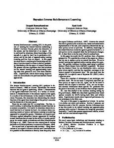
is maximized. Here, t is the time step, and rt is the reward at time step t. The policy π can either be directly learned from the agent-environment interactions, or indirectly through the learning of a value function. All RL methods can be thought of as ways to maximize this expected sum of rewards accumulated over time as the agent interacts with the environment. The standard RL architecture is depicted in Figure 2.1.

F IGURE 2.1: The general RL architecture

In order to allow the agent to act such that more importance is given to immediate rewards, the rewards may be weighted by a discount factor γ ∈ (0, 1]. In such cases, the objective becomes the maximization of the expected sum of discounted rewards, as follows: E

∞ X

γ k rt+k+1

(2.2)

k=0

The greater the value of γ, the more far-sighted the RL agent becomes. A low value of γ would result in the agent being short-sighted in nature, aiming to optimize only its short term behavior. In addition, such a weighting also ensures that the sum of rewards obtained by an agent over an infinite horizon, remains bounded. In general, RL agents continuously and endlessly interact with their environment, adapting to different situations and new information gathered through exploration. Such a setting is referred to as the continual mode of learning in RL. However, if the environment contains a terminal state, then the learning can be divided into multiple episodes. Each episode terminates either after the agent visits a terminal state or after a predefined number of agent-environment interactions. Such a setting is referred to as episodic learning in RL.

2.1. Reinforcement Learning

9

Much of the RL framework is based on Markov decision processes, which is discussed later in this chapter. We subsequently also discuss related topics such as value functions and the idea of approximating them, off-policy learning and other related topics.

2.1.1

Markov Decision Process

A key concept underlying a majority of RL algorithms is the Markov property. The Markov property is respected if the state and reward at the current time step depend only on the previous state and action. Markov decision processes (MDPs) are a special class of RL problems, and provide the theoretical framework for most modern RL algorithms. An MDP is a tuple hS, A, T , Ri, where S is the set of all possible states, A is the action space containing the set of all possible actions, T : S × A × S ⇒ [0, 1] is the transition function which determines the transition probabilities associated with each transition, and R is the reward function which determines the scalar reward associated with each state-action pair. In RL, agent-environment interactions occur to result in a sequence of states, actions and rewards. For example, if the agent starts in state s1 , and takes action a1 , it receives the next state s2 and the reward r2 from the environment. The transition from s1 to s2 as a result of taking action a1 is governed by the transition function T , which outputs a probability distribution over the next state, given the current state s1 and action a1 . All the RL algorithms in this dissertation assumes that the agent operates in an unknown MDP with an action set of finite size. The state space associated with the MDP could be arbitrarily large, in which case it becomes impractical to learn the associated values or action-values. This problem can be resolved using function approximation, which is described in a later section in this chapter.

2.1.2

Value Functions

The objective of RL agents is to learn optimal behaviors in the environments they interact with. RL fulfills this objective by learning a policy π : S × A → [0, 1] that maps states to actions. The policy can be inferred by learning the value function, which can be roughly interpreted as the usefulness of being in a particular state (state value function V ) or of being in a state and taking a particular action (state-action value function Q). These value/action-value functions are learned by bootstrapping, usually from an initially arbitrary estimate, which is repeatedly updated as and when the agent interacts with its environment.

10


The state value function V π (s) at a state s is indicative of the expected sum of rewards starting from state s, and following policy π. Hence, it can be considered to be a mapping between states and expected returns (sum of rewards). That is, V π : S → R. Similarly, the state-action value function Qπ (s, a) is indicative of the amount of rewards that the agent can expect to accumulate starting from state s, having taken an action a, and following a policy π thereafter. That is, Qπ : S × A → R.

2.1.3

Off-Policy Learning

In RL, an agent interacts with its environment using some policy, referred to as its behavior policy µ. The objective however, is to learn an optimal policy with respect to maximizing the expected sum of some predefined rewards. Such a policy is referred to as the target policy π. When the agent’s behavior policy is the same as the target policy, these classes of RL algorithms are called on-policy. When the behavior and target policies differ from each other, it is called off-policy learning. In cases of high degrees of mismatch between the behavior and target policies in off-policy learning, obtaining a good estimate of the target policies may still be challenging. To a certain extent, this mismatch can be corrected for by using techniques such as importance sampling (Rubinstein and Kroese, 2016). The probabilities of choosing a particular action at in a particular state st is computed for both policies, and their ratio is computed as follows: ρIS =

π(st , at ) , µ(st , at )

(2.3)

where ρIS is the importance sampling ratio. This ratio can be used in the value function update equation in order to account for the fact that the policy µ differs from π. Off-policy learning approaches can be very powerful due to the fact that it enables an agent to learn its optimal value function even when it takes non-optimal actions. This implies that multiple tasks can be simultaneously learned using off-policy approaches. In this dissertation, we make extensive use of off-policy learning in this context.

Q-learning One of the primary off-policy mechanisms through which the efficiency of experiences is improved in this dissertation is by the simultaneous learning of multiple value functions using Q-learning. The update equation for the tabular case (when the states and actions are discrete) is shown in Equation (2.4).


Q(s, a) ← Q(s, a) + α[r(s, a) + γmaxa0 Q(s0 , a0 ) − Q(s, a)]

11

(2.4)

where Q(s, a) is the Q-value corresponding to state s and action a. s0 is the next state, and a0 is a bound variable that can represent any action in the action space A. α is the learning rate and γ is the discount factor. In Equation (2.4), the term r(s, a) + γmaxa0 Q(s0 , a0 ) is basically the sum of the current reward r(s, a) and the optimistic discounted estimate of future rewards γmaxa0 Q(s0 , a0 ). Hence the term r(s, a) + γmaxa0 Q(s0 , a0 ) − Q(s, a) can be thought of as the change in the estimate of future rewards, starting from state s and action a. This term is referred to as the temporal difference (TD) error δ. In general, learning is characterized by a reduction of the absolute values of TD errors over time. Hence, the monitoring of TD errors can be used as a way to ensure that learning is taking place successfully.

2.1.4

Function Approximation

For large or continuous state spaces, it becomes infeasible to store the value function corresponding to each state or state-action pair. Hence, function approximators capable of approximating these value functions are needed for learning to occur in a scalable manner, especially in large or continuous state-space environments. Generally, any type of function approximator used can be used to approximate the value function of an RL task. The use of deep neural networks as a function approximator has recently gained popularity due to its ability to handle high dimensional problems, as well as due to the easy availability of inexpensive and powerful computing hardware. However, RL algorithms using deep neural network function approximators are known to be computationally expensive and extremely sample inefficient. These aspects make them unfavorable for the purpose of this dissertation, especially in applications involving the deployment of online learning algorithms on robotics platforms such as the EvoBots. Hence, in this dissertation, we approximate the value functions by linear function approximation. In this approach, a set of weight vectors are learned from the agent-environment interactions, which, when linearly weighted with the feature vector, enables us to recover the corresponding value function. The following sub-section describes the Q-λ algorithm, which extends the tabular Q-learning approach to the continuous case by learning a set of linear weights.

12


Q-learning with linear function approximation The Q-λ algorithm is an extension of tabular Q-learning to continuous state spaces. In Q-λ, the Q functions are learned by updating weight vectors w after each interaction with the environment. It also involves the use of eligibility traces (Sutton, 1988), which helps speed up the propagation of learned information. Here, replacing traces are used for the Q-λ updates (Singh and Sutton, 1996). The update equations for the Q-λ algorithm are mentioned below:

δ = R(s, a) − Q(s, a)

(2.5)

δ ← δ + γmaxa0 Q(s0 , a0 )

(2.6)

w ← w + αδe

(2.7)

e ← γλe

(2.8)

where w is the weight vector, e is the eligibility trace vector, λ is the trace decay rate parameter. The elements of the eligibility trace vector (replacing traces) are initialized with a value of 1 if the corresponding features are active. Otherwise, they are initialized with a value of 0. The Q-values mentioned in equations (2.6) and (2.5) are stored in the form of weight vectors as: Q(s, a) =

X

wi

(2.9)

i∈Fact (s,a)

where Fact (s, a) is the set of active binary features for an agent in state s, taking an action a. A more detailed summary of the algorithm can be found in (Sutton and Barto, 1998b).

2.1.5

Deep Reinforcement Learning

Apart from linear function approximators, the task of approximating the Q function can also be carried out using general function approximators such as deep neural networks (Rumelhart, Hinton, and Williams, 1985). In a very broad sense, deep reinforcement learning (DRL) (Mnih et al., 2015; Silver et al., 2016) algorithms refer to the family of RL algorithms where a deep neural network in used for the task of function approximation. Conceptually, DRL algorithms are not fundamentally different from


13

RL, although they require specific modifications in order to ensure stable learning. Although these algorithms are very popular, and have been shown to be able to handle high dimensional problems remarkably well, they suffer from the drawback that they are extremely sample inefficient. Due to this limitation, applications using these algorithms are restricted to virtual environments such as the ATARI platform (Mnih et al., 2013), where the cost of acquiring samples is not very large. For real world tasks such as robotics, DRL would not have the luxury of experiencing millions of interactions with the environment. In addition to this, DRL approaches are also computationally intensive, and require powerful computing equipment, which may not always be a feasible option for physical platforms. Apart from this, the dimensionality of the navigation problem that is considered in this dissertation is not very large. Hence, DRL did not seem to provide significant advantages over simpler function approximators. Due to these reasons, in this dissertation, we primarily focus on non-DRL approaches to RL. However, the methods developed here could also be applied to DRL, if needed. Discussions regarding this aspect have been included in Chapters 3, 4 and 5, where appropriate.

2.1.6

Exploration-Exploitation Dilemma

In many RL algorithms, the agent needs to make a choice between exploiting its current estimate of the value function, and taking exploratory actions to learn more about its environment. Exploitation actions may lead to the accumulation of a high sum of rewards over the agent’s lifetime, but exploratory actions are needed to learn a good estimate of the value function in the first place. In general, it is good to always have some small, but non-zero probability of taking exploratory actions. Doing so enables an agent to adapt to its environment, which may have changed over time. Selecting exploratory actions may also help the agent discover new and more optimal policies. Exploration strategies may be either directed of undirected (Thrun, 1992a). Directed exploration strategies choose exploratory actions based on some previously gathered information (for example, based on the previous states visited, the frequency or recency of visits, the value function itself etc.,) regarding the task at hand. These approaches are usually superior, but require more information and their implementation is computationally more intensive. Although RL literature contains several other sophisticated strategies (McFarlane, 2018) for balancing this exploration-exploitation trade-off, in this dissertation, we mainly use undirected exploration strategies. Particularly, we follow the simple, but popular approach of -greedy exploration. In this approach, we simply define a parameter , with a probability of which, an exploratory action is executed.

14


Consequently, with a probability of 1 − , the agent chooses a greedy action, exploiting its estimates of the value function. Optionally, the exploration parameter can be decreased over time, such that the probability of taking exploratory actions decreases with the number of iterations. Another common approach for balancing this trade-off is the Boltzmann/softmax exploration strategy (Thrun, 1992a), in which the tendency for exploration is controlled by a temperature parameter, which continuously decreases over time.

2.1.7

Experience Replay

In traditional RL approaches, an agent takes actions in its environment, receives state and reward feedback, using which, it updates its value functions. However, information regarding these completed interactions is discarded, and is not stored for later use. Experience replay (Lin, 1992) is an approach for accelerating the learning speed of an RL agent, in which previous transitions (states, actions and rewards) are stored in a replay buffer for later use. These transitions are then randomly picked and presented to the agent from time to time, based on which the agent updates its value function. This approach of recycling previously experienced transitions allows the correlations between subsequent transitions to be broken, making it closer to an independent and identical distribution (IID) setting, thereby allowing the agent to better learn the associated value function through stochastic gradient descent. In addition, experience replay allows multiple passes of the value function update equation with the same data, which helps accelerate learning. This simple idea is of significant use to off-policy RL approaches, particularly those using deep neural network function approximators.

2.2

Clustering

Clustering is a method of discovering patterns in data, based on which the data can be divided into distinct groups. It can be a powerful tool, as many clustering approaches are carried out iteratively and in an unsupervised manner. That is, labeled data is not needed for these groups or clusters to be discovered. In this dissertation, we primarily make use of two such clustering approaches: k-means clustering and self-organizing maps (SOM). These approaches are used in conjunction with RL in chapters 3 and 5 to equip agents with a greater degree of autonomy by allowing them to exploit discovered patterns in the feature and task space respectively. We describe these clustering mechanisms in detail in the remainder of this chapter.

2.2. Clustering

2.2.1

15

k-means clustering

The k-means clustering algorithm is designed to divide n observations into k (with k ≤ n) different groups or clusters such that similar observations become associated with the same cluster. The algorithm is unsupervised (that is, it does not need the observations to be labeled), but requires the specification of the number of desired clusters k. The algorithm works by first randomly assuming the k cluster centroids (C1 ...Ci ...Ck ), which are iteratively updated as observations are presented to it. The objective of the clustering approach is to minimize the distance between each observation and its associated centroid, such that the sum of distances: k X n X

Oi ||Cj

(2.10)

j=1 i=1

is minimized, where Oi ||Cj denotes the distance between the ith observation Oi and the j th centroid Cj . Usually the distance metric used in these computations is the Euclidean distance, although other distance metrics may also be used. With each observation, the distance to each of the k cluster centroids is computed. The given observation is assigned to the cluster, whose centroid is closest to it. Next, each centroid is recomputed based on its updated members. The process repeats until a stopping criteria is met (that is, no observations change clusters, the change in the cluster centroids is negligible for a certain number of iterations, or some maximum number of iterations is reached). One of the demerits of the k-means algorithm is the requirement of specifying k beforehand. In Chapter 3, we relax this requirement by introducing an adaptive version of the k-means algorithm, in which the value of k is automatically determined, and modified if required. This approach is used to discover patterns in the feature space of the RL agent, allowing it to anticipate goal locations for potential future tasks.

2.2.2

Self-organizing maps

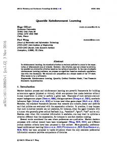
A self-organizing map (SOM) (Kohonen, 1998) is a type of unsupervised neural network used to produce a low-dimensional representation of its high-dimensional training samples. Typically, a SOM is represented as a two- or three-dimensional grid of nodes. Each node of the SOM is initialized to be a randomly generated weight vector wj of the same dimensions as the input vector. Thus, the SOM is initially composed of a set of n weights w = {w1 ..wj ..wn }, which are subsequently modified by the SOM training process. In Figure 2.2, the nodes of the SOM are initialized as pixel inputs of a

16


random intensity of red, blue or green. Each pixel contains three color channels (corresponding to red, blue and green), which serve as the features for this SOM clustering problem. During the SOM training, an input xi , selected from the set of inputs x = {x1 ..xi ..xm } is presented to the network, and the node wwin that is most similar (among the n nodes) to this input is selected to be the ‘winner’. The winning node is then updated towards the input vector xi under consideration. Other nodes in the neighborhood are also influenced in a similar manner, but as a function of a neighborhood function, which, for example, could be their topological distances to the winner. The general update rule for a node wj in the SOM is as follows: wj ← wj + κh(win, j)d(xi , wj ),

(2.11)

where κ is the learning rate, h(j, k) is a neighborhood function which measures the distance between two SOM nodes j and k, and d(u, v) is an arbitrary distance metric between vectors ~u and ~v of the same dimension. Typically, κ and h(i, j) are also made to decrease with the number of iterations, such that large changes to the SOM nodes become less likely as the training progresses.

F IGURE 2.2: An example of SOM training, where a 2 dimensional grid of pixels is organized as per their red, blue and green channel intensities

The final layout of a trained map is such that adjacent nodes have a greater degree of similarity to each other in comparison to nodes that are far apart. An example of this is shown in Figure 2.2, where the map obtained after SOM training captures the structure of the latent input space. In Chapter 5, we describe a growing variant of the standard SOM architecture described here to help store and represent the multiple behaviors (corresponding to multiple tasks) learned by an RL agent in a continual learning scenario.

2.3. Summary

2.3

17

Summary

This chapter covered fundamental concepts in reinforcement learning, as well as some clustering approaches, which will be useful for understanding the remainder of this dissertation. We discussed the basic outline of reinforcement learning, and introduced related concepts such as MDPs, value functions, function approximation, the explorationexploitation dilemma, off-policy learning and experience replay. Finally, we discussed two clustering approaches, the k-means clustering algorithm and self-organizing maps, which are used in conjunction with reinforcement learning in some of the subsequent chapters.

19

Chapter 3

Learning Priors for Potential Auxiliary Tasks1 In this chapter, we present a methodology that enables a reinforcement learning (RL) agent to make efficient use of its exploratory actions by autonomously identifying possible tasks in its environment and learning them in parallel. The identification of tasks is achieved using an online and unsupervised adaptive clustering algorithm. The identified tasks are learned (at least partially) in parallel using off-policy learning algorithms (Q-learning). Using a simulated agent and environment, it is shown that the converged or partially converged value function weights resulting from off-policy learning can be used to accumulate knowledge about multiple tasks without any additional exploration. We claim that the proposed approach could be useful in scenarios where the tasks are initially unknown, or in real-world scenarios where exploration could be a time and energy intensive process. Finally, the implications and possible extensions of this work are also briefly discussed.

3.1

Introduction

Intelligent agents are characterized by their abilities to learn from and adapt to their environments with the objective of performing specific tasks. Very often, in reinforcement learning (RL) (Sutton and Barto, 1998b), and in machine learning in general, algorithms are structured to be able to fulfill one specific task. For example, in an RL maze solving/navigation task, the goal is usually specified in terms of a particular region in the feature space that is associated with a high reward. In general, environments are likely to contain multiple features, and different regions in the feature space may specify different goals, whose associated tasks could be assigned to the agent to learn. In 1

A majority of the contents of this chapter has been published as an article in the journal Neurocomputing (Karimpanal and Wilhelm, 2017)

20

Chapter 3. Learning Priors for Potential Auxiliary Tasks

real-world scenarios, however, the ability to efficiently learn more than one task during a single deployment could drastically improve the agent’s usefulness. In order to achieve this, the agent would need to be aware of regions in the feature space that could possibly play a role in its future tasks. Embodied artificial agents or intelligent robots are typically equipped with a variety of sensors that enable it to detect characteristic features in its environment. In the context of RL, when such an agent is placed in an unknown environment and is assigned a task, it carries out some form of exploratory behavior in order to first discover a region in the feature space that fulfills this specified goal. Further exploratory actions may help improve its value/action-value function estimates, which in turn lead to improved policies. We shall refer to this original task as the primary task, and to its associated ~ During exploration, feature vector of the goal state as the primary task feature vector (ψ). it is likely that the agent comes across other ‘interesting’ regions which contain features that stand out with respect to the agent’s history of experiences. We shall refer to these ~ and to the associated tasks as auxiliary feature vectors as auxiliary task feature vectors(φ) tasks. Although these regions could be of interest to the agent for future tasks (which are currently unknown), they may be irrelevant to the task at hand. Hence, it is justified for the agent to ignore them and continue performing value function updates for the primary task assigned to it. However, the agent’s future tasks may not remain the same, and a new task assigned to it may correspond to a particular combination of features that it encountered while learning policies for the primary task. In such a case, the fact that this region in the feature space had been previously encountered cannot be leveraged since they were not relevant to the agent at that point of time, and were hence ignored. The above mentioned approach would result in a considerable amount of wasteful exploration. This is because each new task assigned to the agent would require a fresh phase of discovery and learning of the associated feature vector and value functions respectively. A more efficient approach would be to keep track of possible auxiliary tasks and learn them in parallel using off-policy methods (Precup, Sutton, and Dasgupta, 2001; Sutton and Barto, 1998b). In the context of off-policy learning, this can be done by treating the policies corresponding to the auxiliary tasks as target policies, and learning them while executing the behavior policy which is dictated by the primary task. Depending on the tasks, the actions executed by the behavior policy may not be optimal with respect to the auxiliary tasks. However, using off-policy learning, it is possible to at least partially learn the value functions for multiple auxiliary tasks, thereby significantly improving the efficiency of exploration. In applications such as robotics, where exploration is known to be costly in terms of time, energy and other

3.2. Related Work

21

factors, such an approach could prove to be practical. In this chapter, we present a framework in which an unsupervised, adaptive clustering algorithm is designed and used to cluster regions of the feature space into different groups based on the similarity of their associated features. Off-policy methods are used to simultaneously learn target policies corresponding to these clusters, the centroid of each of which is treated as features associated with an auxiliary task. The clustering of features occurs as and when they are seen by the agent while learning the primary task. The value function updates can be performed using suitable off-policy methods, namely, tabular Q-learning, Q- λ (Watkins, 1989) or other more recent off-policy methods (Geist and Scherrer, 2014) such as off-policy LSTD(λ) (Yu, 2010; Lagoudakis and Parr, 2003), off-policy TD(λ) (Precup, 2000; Precup, Sutton, and Dasgupta, 2001), GQ(λ) (Maei and Sutton, 2010) etc., The results presented here, however, are obtained using the Q-λ algorithm. Although auxiliary tasks are discovered while learning the primary task, the primary task itself has a minimal role to play in this process. As long as the agent executes some exploratory actions while learning to perform its primary task, auxiliary task can be discovered and at least partially be learned. In fact, even a highly exploratory policy can be used. These aspects are discussed in further detail in Section 3.5. The aim of the approach proposed here is not to learn all the auxiliary tasks perfectly, but to identify a subset of them via the adaptive clustering algorithm, and learn them at least partially through off-policy learning. Doing so could provide the agent with a good initialization of value function weights so that optimal policies for the identified potential auxiliary tasks could be learned in the future, if needed.

3.2

Related Work

Although off-policy methods such as Q-learning have been well known and widely used over the years, their use for autonomously handling multiple independent tasks has been limited, primarily owing to very few precedents on unsupervised identification of tasks in an agent’s environment. Off-policy approaches with function approximation have also been known to have long standing issues with stability until recently (Sutton et al., 2011). Although approaches for handling multiple independent tasks in parallel are rather limited, a number of multi-objective RL approaches that handle multiple conflicting objectives exist. A comprehensive survey of such methods can be found in (Roijers et al., 2013).

22


The horde architecture of Sutton et al. (Sutton et al., 2011) has been shown to be able to learn multiple pre-defined tasks in parallel using independent RL agents in an offpolicy manner. The knowledge of these tasks is stored in the form of generalized value functions which makes it possible to obtain predictive knowledge relating to different goals of the agent. Modayil et al. (Modayil, White, and Sutton, 2014) and White et al. (White, Modayil, and Sutton, 2012) also focus on learning multiple tasks in parallel using off-policy learning. Apart from this, Sutton et al. (Sutton and Precup, 1998) used off-policy methods to simultaneously learn multiple options (Sutton, Precup, and Singh, 1999b), including ones not executed by the agent. They mention that the motivation for using off-policy methods is to make maximum use of whatever experience occurs and to learn as much as possible from them, which is an idea that is reflected in the work presented in this chapter. In the works mentioned above, the multiple tasks that are learned in parallel are predefined. However, in this chapter, we focus on the case where the agent has no foreknowledge of the tasks in its environment. The tasks are identified by the agent itself via clustering. Hence, the agent learns independently in the sense that as it moves through its environment, it identifies potential tasks and at least partially learns their associated value functions in parallel. A similar approach is seen in Mannor et al. (Mannor et al., 2004), where clustering is performed on the state-space to identify interesting regions. However, their approach was not online and the purpose of their work was to use these regions to automatically generate temporal abstractions. Recent work on hindsight experience replay (HER) (Andrychowicz et al., 2017) has some parallels to the approach described in this chapter. Like HER, our approach also aims at improving sample efficiencies in multiple goal scenarios using off-policy RL algorithms. The approaches are also similar in the sense that they both effectively learn shaping functions which aid the learning of tasks. However, our approach achieves this by learning value functions for a set of tasks, selected based on identified patterns in the feature space. In contrast, HER operates by replaying experiences as if one of the previously experienced states were the goal. One of the key components of our proposed approach is a variant of the k-means clustering algorithm (Hartigan and Wong, 1979; Anderberg, 2014) to cluster features that are characteristic of auxiliary tasks. The approach is similar to that of Bhatia (2004), where an adaptive clustering approach is described. The difference lies in the fact that in our method, in addition to the mean, statistical properties such as the variance and number of members in each cluster are updated online and used for clustering as and when the environment is sensed by the agent.

3.3. Description

23

In general, the algorithm also bears similarities to some aspects of adaptive resonance theory (Carpenter and Grossberg, 2016). The procedure of finding and updating the winning cluster in our approach is similar to that for comparing input vectors to the recognition field, and updating recognition neurons towards the input vector in adaptive resonance theory. Perhaps the main differences are the nature and function of the threshold/vigilance parameter. In our approach, the threshold is related to the variance of the cluster, which varies dynamically as more members are acquired by the clusters. However, in both approaches, the threshold has an effect on the resolution of the clusters. Overall, our clustering approach is simpler, and it is only focused on being able to identify clusters in an online manner, without much consideration to factors such as biological plausibility. The details of the algorithm are discussed further in Section 3.4.

3.3

Description

F IGURE 3.1: The simulated agent and its range sensors

In order to demonstrate the proposed approach for identifying and learning multiple tasks, we consider an agent in a continuous space which contains obstacles, a region lit up by a light source, and a bumpy/rough area. We assume that characteristic features corresponding to these regions can be detected by the agent using its on-board sensors: a set of range sensors, a light detecting sensor, and an inertial motion unit (IMU) to sense changes in surface roughness. A sample of the environment is shown in Figure 3.2. The range sensors on the robot are radially separated from each other by 72 degrees as shown in Figure 3.1, and are capable of sensing the presence of obstacles within 1 unit distance. Initially, the agent has no foreknowledge of the environment, and can move forwards and backwards, sideways and diagonally up or down to either side. In addition to this, it can also hold its current position. Thus, a total of 9 actions (which compose the action

24


set A) are available for execution. These actions are executed sequentially according to the behavior policy, which depends on the primary task assigned to the agent. The time step for action execution is set to be 200ms and the agent’s velocity is set to be 8 units/s for the relevant actions. The environment is chosen to be 30 × 30 in size. The features are a function of the agent’s state in the environment, which is composed of the agent’s (x,y) position and its heading direction. Deriving these features from the agent’s state is critical to learning, and is described below.

3.3.1

Agent Features

The agent is capable of sensing different features in the environment using its sensors. The sensors are simulated to have 5% Gaussian white noise. We shall refer to the resulting feature vector as the environment feature vector (F~e ). Apart from the binary features in (F~e ), additional features are needed in order for the agent to be able to learn policies for navigation tasks. We shall refer to the vector of these features as the agent feature vector (F~a ). Hence, the full feature vector (F~ = F~e ∪ F~a ) for the agent consists of both these feature vector components.

F IGURE 3.2: One of the agent’s policies to navigate to the target location in the simulated environment. The environment contains features such as a region with light, a rough region, obstacles and a target location

3.4. Methodology

25

The feature vector F~e consists of the following: 1. Feature indicating either the presence or absence of obstacles as seen by any of the three range sensors. 2. Feature corresponding to the presence or absence of light 3. Feature corresponding to rough or smooth floor surfaces, as reported by the IMU 4. Feature indicating whether the agent lies within the range of the specified target location The agent feature vector F~a is composed of 100 binary features corresponding to each dimension in the 2-dimensional space. It is concerned with the localization of the agent, and is used for learning the required policies. In F~a , the feature value is equal to 1 for the agent’s current position and 0 for all other positions in the space. Hence, the full feature vector consists of 204 (200 localization and 4 environment) feature elements. Only F~e is passed into the clustering algorithm to identify different regions of interest, whereas the full feature vector is used in the Q-λ update equations.

3.4

Methodology

Section 3.3 described the simulated environment, the agent and the feature vector it is capable of sensing. In this section, we describe the methodology used to identify regions of interest in the feature space and how these regions, when treated as goal locations corresponding to arbitrary auxiliary tasks, can enable the learning of multiple tasks in parallel using an off-policy approach.

3.4.1

Adaptive Clustering

As described, the feature vector sensed by the agent consists of features relating to the environment as well as features for localization of the agent. The agent is initially as~ which is a particular signed an arbitrary primary task, which is specified in terms of ψ, ~ apart from the binary values that each feature can configuration of F~e . In specifying ψ, take, a ‘don’t care’ case is also included. During the task specification, if a primary task feature is associated with the ‘don’t care’ case, it implies that any feature value sensed ~ in the feature space. for that feature is considered acceptable during the search for ψ In learning the primary task, the agent learns a policy that takes it from any arbitrary ~ state in the environment to a state where F~e matches the feature vector described by ψ.

26


As the agent moves through the environment in search of the feature vector specified ~ it is continuously presented with new F~e vectors. Our approach is to cluster by ψ, these features as and when they are seen. The k-means (Romesburg, 2004; Anderberg, 2014) algorithm is a simple and popular algorithm used for unsupervised clustering. However, it requires prior knowledge of the number of clusters present in the feature space. This does not suit our application, as we assume no prior knowledge about the environment. The algorithm was therefore modified in order to make it adaptive, so that new feature vectors that seem different from the others may seed new clusters. This is done by continuously updating statistical properties such as the mean, variance and number of members in each cluster, and by measuring the closeness of the feature elements in F~e to the corresponding feature centroids in the centroid vector ~ν of the different clusters. Each new cluster that is seeded is initially set to have non-zero variance, which we shall refer to as the seed variance. This is done in order to maintain a certain level of uncertainty about the cluster centroids initially. The uncertainty reduces as more number of samples are observed. As the agent moves through the environment, the Euclidean distance between the environment feature vector F~e that it sees, and the centroid vector of each cluster is calculated, and the cluster corresponding to the minimum distance is chosen as the ‘winning’ cluster. Next, the element-wise absolute distance between the centroid of the winning cluster and components of F~e is computed. For each element, if this distance lies within n standard deviations of the centroid of that feature element, then the F~e belongs to that cluster; if not, a new cluster is seeded. So n can be considered a tolerance parameter for the clustering algorithm. Each time a cluster receives a new member, the centroid and variance of each of the j th feature element in the cluster is updated online using the corresponding elements of F~e . The straightforward equations governing the updates are defined by the first and second statistical moments of the sensor measurement in Equation (3.1) and Equation (3.2) respectively. νj ←− (NC ∗ νj + Fej )/(NC + 1)

2

(3.1)

σj 2 ←− (NC ∗ (σj2 + νj2 ) + Fej )/(NC + 1) − νj2

(3.2)

NC ←− NC + 1

(3.3)

where νj and σj 2 are respectively the mean (centroid) and variance of the j th feature element in the cluster, whereas NC is the number of members in cluster C. The structure

3.4. Methodology

27

of the clustering algorithm is summarized in Algorithm 1. Overall, the algorithm serves to cluster the feature space in an unsupervised and adaptive manner without prior knowledge of the number of clusters that exist in the space. The centroid of each of the identified clusters is considered to be representative of the features associated with the goal location of an auxiliary task which is learned in parallel with the primary task using off-policy methods. Algorithm 1 Adaptive clustering algorithm 1:

2: 3: 4: 5: 6: 7: 8: 9: 10: 11:

Inputs: Feature vector F~e , variance threshold parameter n, number of existing clusters k (initially set to 1), existing clusters C and their properties: centroid vector ~ν , standard deviation ~σ (elements initialized with non-zero seed variance for a new cluster) and number of members NCk (initialized to 1 for a new cluster) for i=1:k do di = Euclidean_distance(F~e , ~νi ) end for win = {argmin(d)} j j if |(Fej − νwin )| ≥ n ∗ σwin for each feature Fej in F~e , then k =k+1 F~e ∈ Ck else F~e ∈ Cwin Update the mean and variance of each element in the winning cluster j j νwin ←− (NCwin ∗ νwin + Fej )/(NCwin + 1) 2

2

2

2

j j j j σwin ←− (NCwin ∗ (σwin + νwin ) + Fej )/(NCwin + 1) − νwin 12: Update the number of members in the winning cluster NCwin ←− NCwin + 1 13: end if

3.4.2

2

Off-Policy Learning

The clustering algorithm described in Section 3.4.1 groups feature vectors F~e into different clusters in an adaptive and unsupervised manner. As and when each new cluster is seeded, an associated set of weight vectors (to learn the corresponding Q function) is also created. The overall algorithm is summarized in Algorithm 2.

28


Algorithm 2 Identifying and learning tasks using clustering and off-policy methods 1:

~ variance threshold parameter n, number Inputs: Primary task feature vector (ψ), of existing clusters k (initially set to 1), starting state (xstart ), weight vector wO , Q-λ parameters for primary task: discount factor (γ), learning rate (α), exploration parameter (), decay rate parameter for eligibility traces (λ) number of iterations for Q-λ (N _iter), existing clusters C and their properties: mean (vector of centroids) ~ν , standard deviation ~σ and number of members N

2: 3: 4: 5:

for i=1:N _iter do state=xstart F~e = GetFeaturesFromState(state) ~ do while F~e 6= ψ

7:

Take -greedy action and visit new state xnew F~enew =GetFeaturesFromState(xnew )

8:

Cluster F~enew using algorithm 1

9:

if New clusters are formed, then

10:

Seed wnew_cluster and update k

6:

11: 12: 13:

end if ~ then if F~enew == ψ, reward=high

14:

elsereward=low

15:

end if

16:

Update wO using Q-λ equations

17:

for j=1:k do ~ νj φ=~

18: 19:

~ then if F~enew == φ

20:

reward(j)=high

21:

else reward(j)=low

22: 23:

end if

24:

Update wj using Q-λ equations

25:

end for

26:

x = xnew F~e =F~enew

27: 28: 29:

end while end for

3.5. Results

3.5

29

Results

In this section, we summarize the results obtained by applying the methodology described in Section 3.4 to the agent and environment described in Section 3.3. The sample environment used for the simulations are shown in Figures 3.2 and 3.5. In these figures, larger markers corresponding to the agent’s path signify points closer to the starting position of the agent. The configuration of the obstacles in the environment is set up to be similar to the ‘puddle world’ problem (Sutton, 1996), in the sense that in order for the agent to navigate to the required location, it may need to temporarily move away from its target location. The agent executes an - greedy policy while learning a primary task, during which it senses features F~e in its environment, and continuously sorts them into new or existing clusters as dictated by the equations in Algorithm 1. Figure 3.3 shows the clusters identified by the algorithm after the Q-λ algorithm is applied to learn the primary task of navigating to the target location. In Figure 3.3, a total of 7 clusters can be seen, each marked with a distinct texture and number. It is also seen that regions that have an overlap of different types of features are sorted as different clusters. For example, the region near the top right corner of Figure 3.3 contains a cluster (marked as cluster 7) which corresponds to the overlap between an area around the target location and the presence of an obstacle. In Figure 3.4, it is seen that during episode 1, this overlapping

F IGURE 3.3: Different clusters detected by the agent for the environment shown in Figure 3.2

area is not distinguished as a separate cluster. This changes as the episodes proceed,

30


and the overlapping area is eventually identified as a distinct cluster after episode 6. A similar overlap exists (marked as cluster 6 in Figure 3.3) around the area with high floor roughness near the top left corner of the environment. This shows that with a larger number of samples, the clustering algorithm is capable of distinguishing different combinations of feature elements in the feature space in an unsupervised manner.

F IGURE 3.4: Progression of cluster formation with episodes of the Q-λ algorithm

TABLE 3.1: Average number of clusters formed as clustering parameters seed variance and clustering tolerance (n) are varied

seed variance=0.1 seed variance=1 seed variance=100

n=0.1 6.82 6.77 6.49

n=0.5 6.59 6.43 6.36

n=1 6.65 6.33 6.51

n=1.1 1.93 1.47 1.63

n=1.5 1.36 1.19 1.06

n=2 1.39 1 1

Table 3.1 shows the average number of clusters identified as the seed variance and the clustering tolerance n are varied. The values shown are compiled for 50 Q-λ runs with an exploration parameter = 0.3 for 1000 episodes. The other parameters are the

3.5. Results

31

learning rate α = 0.3, the discount factor γ = 0.9 and the eligibility trace decay rate parameter λ = 0.9. These parameters were kept constant for the Q-λ runs. The results shown in Table 3.1 suggest that the clustering is sensitive to the clustering tolerance, as we may have expected. The lower the value of n, the larger is the number of clusters identified. As per algorithm 1, the condition for new clusters to be formed is: |(F − ν)| ≥ nσ

(3.4)

where F is the value of the feature element and ν and σ are the mean and standard deviation of the associated ‘winning’ cluster. From Chebyshev’s inequality, the probability of clusters forming is bounded by: P (|(F − ν)| ≥ nσ) ≤ 1/n2

(3.5)

When n ≤ 1, the term on the right hand side of Equation (3.5) is ≥ 1. Since probabilities cannot exceed 1, all cases of n ≤ 1 are equivalent in this sense. When n > 1, the probability reduces, and the clustering performance drops. This could provide some explanations for the trends seen in Table 3.1. It also suggests that the clustering tolerance n should ideally be set to a value ≤ 1 if clusters are to be identified effectively. In addition to this, the performance of the clustering algorithm is observed to be more or less independent of the seed variance. This is because the variance of each cluster is continuously updated with each visit to a state. As more samples are obtained, the initial seed variance assigned to a cluster is quickly corrected to be closer to its true value. For the given environment and agent, the clusters were mostly identified during the early episodes of Q-learning. Figure 3.4 shows a typical progression of cluster formation with the number of episodes. The clusters identified by the adaptive clustering algorithm are passed on as goal features for auxiliary tasks, which are in turn learned using off-policy learning. The centroid vector of these clusters, which describe the features represented by the cluster are then used to construct the feature vectors of the goal states of the respective auxiliary ~ tasks (φ). For the case of feature vectors F~e with a large number of elements, the number of clusters identified is likely to be large. For example, when 60 additional features were added to the environment feature vector described in Section 3.3, a total of 748 different clusters were formed. In such cases, it may be more practical to choose a certain number of clusters based on some predetermined criteria, and learn their associated policies. The basis for this choice, however, is a topic that requires further research. An example of one such basis could be the average value of the temporal difference (TD)

32


error across the state-action space, with auxiliary tasks corresponding to lower average error values being preferred. The hypothesis is that since the reward structures for the different tasks are similar, tasks with the lowest average TD error are likely to have have been learned more reliably. Hence, the tasks could be prioritized in this manner according to the reliability of their associated Q-functions. However, in the work presented in this chapter, we deal with a relatively small number of auxiliary tasks, and their corresponding value functions are updated merely in the order in which the tasks are discovered.

F IGURE 3.5: Trajectories corresponding to the policies for different tasks learned by executing the behavior policy for the original task

Once the clustering algorithm identifies an auxiliary task goal feature, its corresponding weight vectors are initialized, and its value function is learned by making use of whatever experience could be gained from the agent’s behavior policy. The reward structure for the auxiliary tasks is assumed to be similar to that of the primary task, ~ instead of ψ. ~ At except that for the former, high rewards become associated with φ, the end of each episode of learning, the agent’s starting position is reset randomly to a non-goal state. As the agent executes actions according to its behavior policy, it updates the value function of the primary task. In addition to this value function update,

3.5. Results

33

the value functions of the auxiliary tasks are also simultaneously updated. In this way, the agent’s interactions with its environment are used to learn multiple tasks simultaneously. Table 3.2 shows the average returns obtained at different stages of learning, when the behavior policy is - greedy with respect to the primary task. Each of the clusters shown in Figure 3.3 represents the goal feature of an auxiliary task, but only the values for meaningful auxiliary tasks such as navigating to the regions with light or with a rough area have been tabulated. The values in Table 3.2 are obtained such that at the end of each episode, the average return for a particular task is computed through separate evaluation runs. In general, for a given target policy, measuring the returns as the agent executes its behavior policy may not be indicative of how well the target policy has been learned, especially if it differs considerably from the behavior policy. By computing returns using evaluation runs, at any point of time, the extent to which a target policy has been learned can be assessed, irrespective of the behavior policy used to learn it. In each of these evaluation runs, the agent is allowed to execute nga (= 100) greedy actions for ntrials (= 100) trials, each trial starting from a randomly selected state. The average accumulated reward per trial is reported as the return corresponding to that episode. That is, the average return corresponding to the k th episode gk is given by:

ntrials ga P nP

gk =

i=1 j=1

ntrials

rij (3.6)

Where rij is the reward obtained by the agent in a step corresponding to the greedy action j, in trial i. As observed from Table 3.2, as the episodes proceed, the returns increase not only for the primary task, but also for the auxiliary tasks. In general, greedier behavior policies result in higher returns for the primary task. This is expected, as the behavior policy is -greedy with respect to the primary task. For the auxiliary tasks, however, this may not be the case. The light task for example, benefits from the behavior policy being more exploratory, whereas its effect on the performance of the rough task is not as pronounced. Figure 3.5 shows some of the sample learned trajectories for both the primary task as well as the two selected auxiliary tasks. The agent identified regions in the feature space as goal features of auxiliary tasks, and simultaneously learned their associated action-value functions through off-policy methods. Policies corresponding to the auxiliary tasks were learned even though the agent’s actions were dictated by its primary task. If each of the ‘N’ auxiliary tasks were to be learned sequentially using Q-learning, ‘N’ additional phases of exploration and learning would have been required. Here, the value function for all the auxiliary tasks are learned at least partially from the experience gained while learning to perform the primary task. In this manner, the efficiency

34

Chapter 3. Learning Priors for Potential Auxiliary Tasks TABLE 3.2: Average returns at different stages of learning (episodes 0, 100, 300 and 1000 ), with different exploration parameters, for the primary and selected auxiliary tasks, over 30 runs No. of episodes 0

100

300

1000

Tasks Primary task Light task Rough task Primary task Light task Rough task Primary task Light task Rough task Primary task Light task Rough task

=0.1 -2490 -2571 -2247 -433.3 276.5 -64.11 1634 689.9 1758 3128 766.8 2244

=0.5 -2453 -2414 -2168 -1107 1180 780.1 824.8 1954 1332 1031 2247 2430

=0.9 -2463 -2280 -2186 -275.7 2423 1351 1055 2884 1914 1316 3075 2226

of exploration is largely improved, irrespective of whether the agent’s behavior policy is greedy or highly exploratory. In order to further evaluate the utility of the proposed method, experiments are performed to measure the initial number of steps required for reaching the goal locations for different tasks, without and with the priors obtained using our described method. These experiments are performed for different values of exploration parameter , and the results are shown in Figure 3.6. As seen from Figure 3.6, the initial number of steps to the respective goal locations is significantly reduced when the learned priors are employed.

3.6

Discussion

The methodology described in this chapter proposes an approach to at least partially learn the value functions of possible auxiliary tasks using the agent’s behavior policy. The auxiliary tasks are identified using an adaptive clustering algorithm. This algorithm identifies clusters in an online manner, and is thus suitable for applications such as robotics. An example of this is depicted in Figure 3.7, where the clustering algorithm is deployed on the EvoBot platform (Karimpanal et al., 2017) (further details regarding the platform can be found in Appendix A) to expose the distribution of features in an environment, approximately 1.4 m×1.4 m in size. Figure 3.7 (a) shows an overhead view of the environment containing distinct features in certain locations (marked by the blue, green and yellow markers), along with obstacle features, which are detected when the robot is close (≤ 30 cm) to the walls. This

3.6. Discussion

35

(a) Primary Task

2000

Without priors With priors

Initial number of steps to goal

1000

0 0.1

0.5

0.9

(b) Light Task

2000

1000

0 0.1

0.5

0.9

(c) Rough Task

2000

1000

0 0.1

0.5

0.9

Exploration parameter

F IGURE 3.6: Initial number of steps to reach the respective goal locations for different tasks, for different values of , with and without learned priors. The results are computed over 30 runs.

environment is explored using the EvoBot platform, which identifies clusters of distinct features using the adaptive clustering algorithm described in Algorithm 1. The 7 identified clusters, corresponding to distinct feature regions, are depicted in Figure 3.7 (b). The identification of these distinct clusters could be useful in a number of ways. Treating each cluster centroid as the goal feature of some arbitrary auxiliary task, and learning their associated value functions simultaneously, is just one of them. For example, in Figure 3.7, the identified clusters could simply be used to learn more about the feature distribution in the environment. Such distributions could be useful for generating informative maps, which could subsequently be used for navigation and planning. Auxiliary tasks identified in this manner may or may not be of relevance to the agent in the future, but they are learned anyway. Since exploration is an energy and time expensive process in real-world applications, the described method could prove to be beneficial, as it could obviate the need for a fresh phase of discovery and learning when

36


F IGURE 3.7: (a) Overhead view of an environment (∼1.4 m×1.4 m) containing features such as obstacles (walls), and feature-distinct regions marked by the blue, green and yellow regions. (b) The corresponding feature distribution, obtained after the environment is explored by the EvoBot.

the agent’s primary task is changed. This approach could be useful especially in scenarios where the environment is feature-rich and the agent’s task is not set to be fixed. Off-policy learning enables parallelization of learning by making use of whatever experience occurs. Further, it scales only linearly with the number of auxiliary tasks. Hence it may be justified to learn at least a small number of the identified auxiliary tasks in parallel. The methods described here could potentially be sped up by incorporating abstraction techniques such as tile coding (Sutton, 1996; Whiteson, 2007). However, while dealing with multiple tasks, it should be kept in mind that a good representation for one task may not be useful for another. In other words, useful representations are functions of the tasks themselves. This insight may help guide the development of more flexible abstraction and representation schemes. As demonstrated in Section 3.5, the value function weights, even if partially converged,

3.7. Conclusion

37

can make good starting points for carrying out subsequent Q- learning episodes if improvements in the value function estimates is needed. This can be useful for transfer learning (Taylor and Stone, 2009) or multi-agent applications (Tan, 1993; Busoniu, Babuska, and De Schutter, 2008), as the value function information of the auxiliary tasks could be communicated to another agent whose primary task is similar in nature to one of the original agent’s auxiliary tasks. This could be a much more efficient approach, as each agent need not explore the environment from scratch. The exploration performed by other agents could be leveraged by subsequent agents to carry out their individual tasks.

3.7

Conclusion

The methodology developed and presented in this chapter demonstrates how discovery and learning of potential tasks in an agent’s environment is possible. Potential tasks are identified using an online, unsupervised and adaptive clustering algorithm. The identified tasks are then learned in parallel using off-policy methods. Both clustering as well as off-policy learning are demonstrated using a simulated agent and environment. The performance of the clustering algorithm with respect to its input parameters is tabulated and the findings are discussed. The clustering algorithm is shown to be capable of identifying most of the distinct regions in the environment during the early episodes of Q- learning. Simulations conducted to validate the utility of this approach reveal that the agent is able to at least partially learn multiple tasks in parallel without any additional exploration. This is especially true when the behavior policy itself is exploratory in nature. The future scope, possible extensions to this work and its applications to fields such as transfer learning and multi-agent systems are also briefly discussed. This approach is targeted at real world applications where the tasks are uncertain or not fixed, or in general, where the cost of exploration is considered to be high. Although the efficiency of our approach depends to some extent on the configurations of task goal locations in the environment, we believe it presents a potential to dramatically improve the efficiency of exploration for an RL agent.

39

Chapter 4

Learning from Sequences of Experiences1 Experience replay is one of the most commonly used approaches to improve the sample efficiency of reinforcement learning algorithms. Unlike the approach described in Chapter 3, where feature similarities in the incoming data are identified and exploited, experience replay improves the sample efficiency by storing and reusing the data from individual transitions from time to time. In this chapter, we propose an approach to select and replay sequences of transitions in order to accelerate the learning of a reinforcement learning agent in an off-policy setting. In addition to selecting appropriate sequences, we also artificially construct transition sequences using information gathered from previous agent-environment interactions. These sequences, when replayed, allow value function information to trickle down to larger sections of the state/stateaction space, thereby making the most of the agent’s experience. We demonstrate our approach on modified versions of standard reinforcement learning tasks such as the mountain car and puddle world problems and empirically show that it enables faster, and more accurate learning of value functions as compared to other forms of experience replay. Further, we briefly discuss some of the possible extensions to this work, as well as applications and situations where this approach could be particularly useful.

4.1

Introduction

Real-world artificial agents ideally need to be able to learn as much as possible from their interactions with the environment. This is especially true for mobile robots operating within the reinforcement learning (RL) framework, where the cost of acquiring 1

A majority of the contents of this chapter has been published as an article in the journal Frontiers in Neurorobotics (Karimpanal and Bouffanais, 2018a)

40

Chapter 4. Learning from Sequences of Experiences

information from the environment through exploration generally exceeds the computational cost of learning (Wang et al., 2016; Adam, Busoniu, and Babuska, 2012; Schaul et al., 2016). Experience replay (Lin, 1992) is a technique that reuses information gathered from past experiences to improve the efficiency of learning. In order to replay stored experiences using this approach, an off-policy (Sutton and Barto, 2011; Geist and Scherrer, 2014) setting is a prerequisite. In off-policy learning, the policy that dictates the agent’s control actions is referred to as the behavior policy. Other policies corresponding to the value/action-value functions of different tasks that the agent aims to learn are referred to as target policies. Off-policy algorithms utilize the agent’s behavior policy to interact with the environment, while simultaneously updating the value functions associated with the target policies. These algorithms can hence be used to parallelize learning, and, thus gather as much knowledge as possible using real experiences (Sutton et al., 2011; White, Modayil, and Sutton, 2012; Modayil, White, and Sutton, 2014). However, when the behavior and target policies differ considerably from each other, the actions executed by the behavior policy may only seldom correspond to those recommended by the target policy. This could lead to poor estimates of the corresponding value function. Such cases could arise in multi-task scenarios where multiple tasks are learned in an off-policy manner. Also, in general, in environments where desirable experiences are rare occurrences, experience replay could be employed to improve the estimates by storing and replaying transitions (state, actions and rewards) from time to time. Although most experience replay approaches store and reuse individual transitions, replaying sequences of transitions could offer certain advantages. For instance, if a value function update following a particular transition results in a relatively large change in the value of the corresponding state or state-action pair, this change will have a considerable influence on the bootstrapping targets of states or state-action pairs that led to this transition. Hence, the effects of this change should ideally be propagated to these states or state-action pairs. If instead of individual transitions, sequences of transitions are replayed, this propagation can be achieved in a straightforward manner. Our approach aims to improve the efficiency of learning by replaying transition sequences in this manner. The sequences are selected on the basis of the magnitudes of the temporal difference (TD) errors (Sutton and Barto, 2011), associated with them. We hypothesize that selecting sequences that contain transitions associated with higher magnitudes of TD errors allow considerable learning progress to take place. This is enabled by the propagation of the effects of these errors to the values associated with other states or state-action pairs in the transition sequence.

4.2. Related Work

41

Replaying a larger variety of such sequences would result in a more efficient propagation of the mentioned effects to other regions in the state/state-action space. Hence, in order to aid the propagation in this manner, other sequences that could have occurred are artificially constructed by comparing the state trajectories of previously observed sequences. These virtual transition sequences are appended to the replay memory, and they help bring about learning progress in other regions of the state/state-action space when replayed. The generated transition sequences are virtual in the sense that

F IGURE 4.1: Structure of the proposed algorithm in contrast to the traditional off-policy structure. Q and R denote the action-value function and reward respectively.

they may have never occurred in reality, but are constructed from sequences that have actually occurred in the past. The additional replay updates corresponding to the mentioned transition sequences supplement the regular off-policy value function updates that follow the real-world execution of actions, thereby making the most out of the agent’s interactions with the environment.

4.2

Related Work

The problem of learning from limited experience is not new in the field of RL (Thrun, 1992b; Thomas and Brunskill, 2016). Generally, learning speed and sample efficiency are critical factors that determine the feasibility of deploying learning algorithms in the

42


real world. Particularly for robotics applications, these factors are even more important, as exploration of the environment is typically time and energy expensive (Bakker et al., 2006; Kober, Bagnell, and Peters, 2013). It is thus important for a learning agent to be able to gather as much relevant knowledge as possible from whatever exploratory actions occur. Off-policy algorithms are well suited to this need as it enables multiple value functions to be learned together in parallel. When the behavior and target policies vary considerably from each other, importance sampling (Rubinstein and Kroese, 2016; Sutton and Barto, 2011) is commonly used in order to obtain more accurate estimates of the value functions. Importance sampling reduces the variance of the estimate by taking into account the distributions associated with the behavior and target policies, and making modifications to the off-policy update equations accordingly. However, the estimates are still unlikely to be close to their optimal values if the agent receives very little experience relevant to a particular task. This issue is partially addressed with experience replay, in which information contained in the replay memory is used from time to time in order to update the value functions. As a result, the agent is able to learn from uncorrelated historical data, and the sample efficiency of learning is greatly improved. This approach has received a lot of attention in recent years due to its utility in deep RL applications (Mnih et al., 2015; Mnih et al., 2016; Mnih et al., 2013; Adam, Busoniu, and Babuska, 2012; Bruin et al., 2015). Recent works (Schaul et al., 2016; Narasimhan, Kulkarni, and Barzilay, 2015) have revealed that certain transitions are more useful than others. Schaul et al. (Schaul et al., 2016) prioritized transitions on the basis of their associated TD errors. They also briefly mentioned the possibility of replaying transitions in a sequential manner. The experience replay framework developed by Adam et al. (Adam, Busoniu, and Babuska, 2012) involved some variants that replayed sequences of experiences, but these sequences were drawn randomly from the replay memory. More recently, Isele et al. (Isele and Cosgun, 2018) reported a selective experience replay approach aimed at performing well in the context of lifelong learning (Thrun, 1996). The authors of this work proposed a long term replay memory in addition to the conventionally used one. Certain bases for designing this long-term replay memory, such as favoring transitions associated with high rewards and high absolute TD errors are similar to the ones described in this chapter. However, the approach does not explore the replay of sequences, and its fundamental purpose is to shield against catastrophic forgetting (Goodfellow et al., 2013) when multiple tasks are learned in sequence. The replay approach described in this chapter focuses on enabling more sample-efficient learning in situations where positive rewards occur rarely. Apart from this, Andrychowicz et al. (Andrychowicz et al., 2017) proposed a hindsight experience replay approach, directed

4.2. Related Work

43

at addressing this problem, where each episode is replayed with a goal that is different from the original goal of the agent. The authors reported significant improvements in the learning performance in problems with sparse and binary rewards. These improvements were essentially brought about by allowing the learned value/Q values (which would otherwise remain mostly unchanged due to the sparsity of rewards) to undergo significant change under the influence of an arbitrary goal. The underlying idea behind our approach also involves modification of the Q-values in reward-sparse regions of the state-action space. The modifications, however, are not based on arbitrary goals, and are selectively performed on state-action pairs associated with successful transition sequences associated with high absolute TD errors. Nevertheless, the hindsight replay approach is orthogonal to our proposed approach, and hence, could be used in conjunction with it. Much like in Schaul et al. (Schaul et al., 2016), TD errors have been frequently used as a basis for prioritization in other RL problems (White, Modayil, and Sutton, 2014; Thrun, 1992c; Schaul et al., 2016). In particular, the model-based approach of prioritized sweeping (Moore and Atkeson, 1993; Seijen and Sutton, 2013) prioritizes backups that are expected to result in a significant change in the value function. The algorithm we propose here uses a model-free architecture, and it is based on the idea of selectively reusing previous experience. However, we describe the reuse of sequences of transitions based on the TD errors observed when these transitions take place. Replaying sequences of experiences also seems to be biologically plausible (Ólafsdóttir et al., 2015; Buhry, Azizi, and Cheng, 2011). In addition, it is known that animals tend to remember experiences that lead to high rewards (Singer and Frank, 2009). This is an idea reflected in our work, as only those transition sequences that lead to high rewards are considered for being stored in the replay memory. In filtering transition sequences in this manner, we simultaneously address the issue of determining which experiences are to be stored. In addition to selecting transition sequences, we also generate virtual sequences of transitions which the agent could have possibly experienced, but in reality, did not. This virtual experience is then replayed to improve the agent’s learning. Some early approaches in RL, such as the dyna architecture (Sutton, 1990) also made use of simulated experience to improve the value function estimates. However, unlike the approach proposed here, the simulated experience was generated based on models of the reward function and transition probabilities which were continuously updated based on the agent’s interactions with the environment. In this sense, the virtual experience generated in our approach is more grounded in reality, as it is based directly on the data collected through the agent-environment interaction. In more recent work, Fonteneau et al. describe an approach to generate artificial trajectories and use them to find

44


policies with acceptable performance guarantees (Fonteneau et al., 2013). However, this approach is designed for batch RL, and the generated artificial trajectories are not constructed using a TD error basis. Our approach also recognizes the real-world limitations of replay memory (Bruin et al., 2015), and stores only a certain amount of information at a time, specified by memory parameters. The selected and generated sequences are stored in the replay memory in the form of libraries which are continuously updated so that the agent is equipped with transition sequences that are most relevant to the task at hand.

4.3

Methodology

The idea of selecting appropriate transition sequences for replay is relatively straightforward. In order to improve the agent’s learning, first, we simply keep track of the state, actions, rewards and absolute values of the TD errors associated with each transition. Generally, in difficult learning environments, high rewards occur rarely. So, when such an event is observed, we consider storing the corresponding sequence of transitions into a replay library L. In this manner, we use the reward information as a means to filter transition sequences. The approach is similar to that used by Narasimhan et al. (Narasimhan, Kulkarni, and Barzilay, 2015), where transitions associated with positive rewards are prioritized for replay. Among the transition sequences considered for inclusion in the library L, those containing transitions with high absolute TD error values are considered to be the ones with high potential for learning progress. Hence, they are accordingly prioritized for replay. The key idea is that when the TD error associated with a particular transition is large in magnitude, it generally implies a proportionately greater change in the value of the corresponding state/state-action pair. Such large changes have the potential to influence the values of the states/state-action pairs leading to it, which implies a high potential for learning. Hence, prioritizing such sequences of transitions for replay is likely to bring about greater learning progress. Transition sequences associated with large magnitudes of TD error are retained in the library, while those with lower magnitudes are removed and replaced with superior alternatives. In reality, such transition sequences may be very long and hence, impractical to store. Due to such practical considerations, we store only a portion of the sequence, based on a predetermined memory parameter. The library is continuously updated as and when the agent-environment interactions take place, such that it will eventually contain sequences associated with the highest absolute TD errors.

4.3. Methodology

45

As described earlier, replaying suitable sequences allows the effects of large changes in value functions to be propagated throughout the sequence. In order to propagate this information even further to other regions of the state/state-action space, we use the sequences in L to construct additional transition sequences which could have possibly occurred. These virtual sequences are stored in another library Lv , and later used for experience replay.

F IGURE 4.2: (a) Trajectories corresponding to two hypothetical behavior policies are shown. A portion of the trajectory associated with a high reward (and stored in L) is highlighted (b) The virtual trajectory constructed from the two behavior policies is highlighted. The states, actions and rewards associated with this trajectory constitute a virtual transition sequence.

In order to intuitively describe our approach of artificially constructing sequences, we consider the hypothetical example shown in Figure 4.2(a), where an agent executes behavior policies that help it learn to navigate towards location B from the start location. However, using off-policy learning, we aim to learn value functions corresponding to the policy that helps the agent navigate towards location T . The trajectories shown in Figure 4.2(a) correspond to hypothetical actions dictated by the behavior policy midway through the learning process, during two separate episodes. The trajectories begin at the start location and terminate at location B. However, the trajectory corresponding to behavior policy 2 also happens to pass through location T , at which point the agent receives a high reward. This triggers the transition sequence storage mechanism described earlier, and we assume that some portion of the sequence (shown by the highlighted portion of the trajectory in Figure 4.2(a)) is stored in library L. Behavior policy 1 takes the agent directly from the start location towards the location B, where it terminates. As the agent moves along its trajectory, it intersects with the state trajectory corresponding to the sequence stored in L. Using this intersection, it is possible to artificially construct additional trajectories (and their associated

46


transition sequences) that are successful with respect to the task of navigating to location T . The highlighted portions of the trajectories corresponding to the two behavior policies in Figure 4.2(b) show such a state trajectory, constructed using information related to the intersection of portions of the two previously observed trajectories. The state, action and reward sequences associated with this highlighted trajectory form a virtual transition sequence. Such artificially constructed transition sequences present the possibility of considerable learning progress. This is because, when replayed, they help propagate the large learning potential (characterized by large magnitudes of TD errors) associated with sequences in L to other regions of the state/state-action space. These replay updates supplement the off-policy value function updates that are carried out in parallel, thus accelerating the learning of the task in question. This outlines the basic idea behind our approach. Fundamentally, our approach can be decomposed into three steps: 1. Tracking and storage of relevant transition sequences 2. Construction of virtual transition sequences using the stored transition sequences 3. Replaying the transition sequences These steps are explained in detail in Sections 4.3.1, 4.3.2 and 4.3.3.

4.3.1

Tracking and Storage of Relevant Transition Sequences

As described, virtual transition sequences are constructed by joining together two transition sequences. One of them, say Θt , composed of mt transitions, is historically successful—it has experienced high rewards with respect to the task, and is part of the library L. The other sequence, Θb , is simply a sequence of the latest mb transitions executed by the agent. If the agent starts at state s0 and moves through intermediate states si and eventually to sj+1 (most recent state) by executing a series of actions a0 ...ai ...aj , it receives rewards r0 ...ri ...rj from the environment. These transitions comprise the transition sequence Θb .

 [S(0 : j) π(0 : j) R(0 : j)] Θb = [S((j − m ) : j) π((j − m ) : j) b

b

if

j ≤ mb

R((j − mb ) : j)] otherwise

(4.1)

4.3. Methodology

47

where: S(x : y) = (sx ...si ...sy ), π(x : y) = (ax ...ai ...ay ), R(x : y) = (rx ...ri ...ry ). We respectively refer to S(x : y), π(x : y) and R(x : y) as the state, action and reward transition sequences corresponding to a series of agent-environment interactions, indexed from x to y (x, y ∈ N). For the case of the transition sequence Θt , we keep track of the sequence of TD errors δ0 ...δi ...δk observed as well. If a high reward is observed in transition k, then:  [S(0 : k) π(0 : k) R(0 : k) ∆(0 : k)] Θt = [S((k − m ) : k) π((k − m ) : k) R((k − m ) : k) t t t

if k ≤ mt ∆((k − mt ) : k)] otherwise (4.2)

where ∆(x : y) = (|δx |...|δi |...|δy |). The memory parameters mb and mt are chosen based on the memory constraints of the agent. They determine how much of the recent agent-environment interaction history is to be stored in memory. It is possible that the agent encounters a number of transitions associated with high rewards while executing the behavior policy. Corresponding to these transitions, a number of successful transition sequences Θt would also exist. These sequences are maintained in the library L in a manner similar to the Policy Library through Policy Reuse (PLPR) algorithm (Fernández and Veloso, 2005). To decide whether to include a new transition sequence Θtnew into the library L, we determine the maximum value of the absolute TD error sequence ∆ corresponding to Θtnew and check whether it is τ -close— the parameter τ determines the exclusivity of the library—to the maximum of the corresponding values associated with the transition sequences in L. If this is the case, then Θtnew is included in L. Since the transition sequences are filtered based on the maximum of the absolute values of TD errors among all the transitions in a sequence, this approach should be able to mitigate problems stemming from low magnitudes of TD errors associated with local optima (Baird, 1999; Tutsoy and Brown, 2016b). Using the absolute TD error as a basis for selection, we maintain a fixed number (l) of transition sequences in the library L. This ensures that the library is continuously updated with the latest transition sequences associated with the highest absolute TD errors. The complete algorithm is illustrated in Algorithm 3.

48


Algorithm 3 Maintaining a replay library of transition sequences 1:

2: 3: 4: 5: 6: 7: 8: 9: 10: 11: 12:

Inputs: τ : Parameter that determines the exclusivity of the library l : Parameter that determines the number of transition sequences allowed in the library ∆k : Sequence of absolute TD errors corresponding to a transition sequence Θk L = {Θt0 ...Θti ...Θtm } : A library of transition sequences (m ≤ l) Θtnew : New transition sequence to be evaluated Wnew = max(∆tnew ) for j = 1 : m do Wj = max(∆tj ) end for if Wnew ∗ τ > max(W ) then L = L ∪ {Θtnew } nt =Number of transition sequences in L if nt > l then L = {Θtnt −l ...Θti ...Θtnt } end if end if

4.3.2

Virtual Transition Sequences

Once the transition sequence Θb is available and a library L of successful transition sequences Θt is obtained, we use this information to construct a library Lv of virtual transition sequences Θv . The virtual transition sequences are constructed by first finding points of intersection sc in the state transition sequences of Θb and the Θt ’s in L. Let us consider the transition sequence Θb : Θb = [S(x : y)

π(x : y) R(x : y)],

and a transition sequence Θt : Θt = [S(x0 : y 0 )

π(x0 : y 0 ) R(x0 : y 0 )

∆(x0 : y 0 )],

Let Θts be a sub-matrix of Θt such that:

Θts = [S(x0 : y 0 )

π(x0 : y 0 ) R(x0 : y 0 )],

(4.3)

4.3. Methodology

49

0

Now, if σxy and σxy0 are sets containing all the elements of sequences S(x : y) and S(x0 : 0

y 0 ) respectively, and if ∃sc ∈ {σxy ∩ σxy0 }, then: S(x : y) = (sx , ...sc , sc+1 , ...sy ), and S(x0 : y 0 ) = (sx0 ...sc , sc+1 ...sy0 ). Once points of intersection have been obtained as described above, each of the two sequences Θb and Θts are decomposed into two subsequences at the point of intersection such that:

" Θb =

Θ1b

# (4.4)

Θ2b

where Θ1b = [S(x : c)

π(x : c) R(x : c)]

and Θ2b = [S((c + 1) : y)

π((c + 1) : y)

R((c + 1) : y)]

Similarly, Θts =

" # Θ1ts Θ2ts

(4.5)

where Θ1ts = [S(x0 : c)

π(x0 : c) R(x0 : c)]

and Θ2ts = [S((c + 1) : y 0 ) π((c + 1) : y 0 )

R((c + 1) : y 0 )]

The virtual transition sequence is then simply: " Θv =

Θ1b Θ2ts

# (4.6)

We perform the above procedure for each transition sequence in L to obtain the corresponding virtual transition sequences Θv . These virtual transition sequences are stored

50


in a library Lv : Lv = {Θv1 ...Θvi ...Θvnv }, where nv denotes the number of virtual transition sequences in Lv , subjected to the constraint nv ≤ l. The overall process for constructing and storing virtual transition sequences is summarized in Algorithm 4. Once the library Lv has been constructed, we replay the sequences contained in it to improve the estimates of the value function. The details of this are discussed in Section 4.3.3. Algorithm 4 Constructing virtual transition sequences 1:

2: 3: 4: 5: 6: 7: 8: 9: 10: 11: 12: 13:

Inputs: Sequence of latest mb transitions Θb Library L containing nt stored transition sequences Library Lv for storing virtual transition sequences for t = 1 : nt do Extract Θts from Θt (Equation (4.3)) Find set of states SI corresponding to the intersection of the state trajectories of Θb and Θts if SI is not empty, then for each state si in SI , do Treat si as the intersection point and decompose Θb and Θts as per Equations (4.4) and (4.5) end for Choose sc from SI such that the number of transitions in Θ1b is maximized end if Use the selected sc to construct the virtual transition sequence Θv as per Equation (4.6) Use library Lv to store the constructed sequence (Lv = Lv ∪ {Θv }) end for

4.3.3

Replaying the Transition Sequences

In order to make use of the transition sequences described, each of the state-actionreward triads {s

a

r} in the transition sequence Lv is replayed as if the agent had

actually experienced them. Similarly, sequences in L are also be replayed from time to time. Replaying sequences from L and Lv in this manner causes the effects of large absolute TD errors originating from further up in the sequence to propagate through the respective transitions, ultimately leading to more accurate estimates of the value function. The transitions are

4.4. Results and Discussion

51

replayed as per the standard Q-learning update equation shown below: Q(sj , aj ) ← Q(sj , aj ) + α[r(sj , aj ) + γ max Q(sj+1 , a0 ) − Q(sj , aj )]. 0 a

(4.7)

Where sj and aj refer to the state and action at transition j, and Q and r represent the action-value function and reward corresponding to the task. The variable a0 is a bound variable that represents any action in the action set A. The learning rate and discount parameters are represented by α and γ respectively. The sequence Θts in Equation (4.6) is a subset of Θt , which is in turn part of the library L and thus associated with a high absolute TD error. When replaying Θv , the effects of the high absolute TD errors propagate from the values of state/state-action pairs in Θ2ts to those in Θ1b . Hence, in case of multiple points of intersection, we consider points that are furthest down Θb . In other words, the intersection point is chosen to maximize the length of Θ1b . In this manner, a larger number of state-action values experience improvements brought about by replaying the transition sequences. Algorithm 5 Replay of virtual transition sequences from library Lv 1:

2: 3: 4: 5: 6: 7: 8: 9:

4.4

Inputs: α : learning rate γ : discount factor Lv = {Θv0 ...Θvi ...Θvnv } : A library of virtual transition sequences with nv sequences for i = 1 : nv do nsar =number of {s a r} triads in Θvi j=1 while j ≤ nsar do Q(sj , aj ) ← Q(sj , aj ) + α[r(sj , aj ) + γ maxa0 Q(sj+1 , a0 ) − Q(sj , aj )] j ←j+1 end while end for

Results and Discussion

We demonstrate our approach on modified versions of two standard reinforcement learning tasks. The first is a multi-task navigation/puddle-world problem (Figure 4.3), and the second is a multi-task mountain car problem (Figure 4.6). In both these problems, behavior policies are generated to solve a given task (which we refer to as the primary task) relatively greedily, while the value function for another task of interest (which we refer to as the secondary task) is simultaneously learned in an off-policy

52


manner. The secondary task is intentionally made more difficult by making appropriate modifications to the environment. Such adverse multi-task settings best demonstrate the effectiveness of our approach and emphasize its advantages over other experience replay approaches. We characterize the difficulty of the secondary task with a difficulty ratio ρ, which is the fraction of the executed behavior policies that experience a high reward with respect to the secondary task. A low value of ρ indicates that achieving the secondary task under the given behavior policy is difficult. In both tasks, the Q-values are initialized with random values, and once the agent encounters the goal state of the primary task, the episode terminates.

4.4.1

Navigation/Puddle-World Task

F IGURE 4.3: Navigation environment used to demonstrate the approach of replaying transition sequences

In the navigation environment, the simulated agent is assigned tasks of navigating to certain locations in its environment. We consider two locations, B and T , which represent the primary and secondary task locations respectively. The environment is set up such that the location corresponding to high rewards with respect to the secondary task lies far away from that of the primary task (see Figure 4.3). In addition to this, the accessibility to the secondary task location is deliberately limited by surrounding it with obstacles on all but one side. These modifications contribute towards a low value of ρ, especially when the agent operates with a greedy behavior policy with respect to the primary task.


53

The agent is assumed to be able to sense its location in the environment accurately, and can detect when it ‘bumps’ into an obstacle. It can move around in the environment at a maximum speed of 1 unit per time step by executing actions to take it forwards, backwards, sideways and diagonally forwards or backwards to either side. In addition to these actions, the agent can choose to hold its current position. However, the transitions resulting from these actions are probabilistic in nature. The intended movements occur only 80 % of the time, and for the remaining 20 %, the x- and y-coordinates may deviate from their intended values by 1 unit. Also, the agent’s location does not change if the chosen action forces it to run into an obstacle. The agent employs Q-learning with a relatively greedy policy ( = 0.1) that attempts to maximize the expected sum of primary rewards. The reward structure for both tasks is such that the agent receives a high reward (100) for visiting the respective goal locations, and a high penalty (−100) for bumping into an obstacle in the environment. In addition to this, the agent is assigned a living penalty (−10) for each action that fails to result in the goal state. In all simulations, the discount factor γ is set to be 0.9, the learning rate α is set to a value of 0.3 and the parameter τ mentioned in Algorithm 3 is set to be 1. Although various approaches exist to optimize the values of the Q-learning hyperparameters (Even-Dar and Mansour, 2003; Tutsoy and Brown, 2016a; Garcia and Ndiaye, 1998), the values were chosen arbitrarily, such that satisfactory performances were obtained for both the navigation as well as the mountain-car environments. 3000

ρ = 0.0065 Average return

2000

1000

0

Experience replay: transition sequences Experience replay: uniform random sampling Prioritized experience replay (proportional) Q-learning without experience replay

-1000 0

200

400

600

800

1000

Number of episodes

F IGURE 4.4: Comparison of the average secondary returns over 50 runs using different experience replay approaches as well as Q-learning without experience replay in the navigation environment. The standard errors are all less than 300. For the different experience replay approaches, the number of replay updates are controlled to be the same.

In the environment described, the agent executes actions to learn the primary task. Simultaneously, the approach described in Section 4.3 is employed to learn the value functions associated with the secondary task. At each episode of the learning process,

54


the agent’s performance with respect to the secondary task is evaluated. The average return corresponding to each episode in Figure 4.4 is computed using Equation (3.6), as described in Chapter 3. The mean of these average returns over all the episodes is reported as Ge in Table 4.1. That is, N E P

Ge =

gk

k=1

NE

Where gk is the average return (computed using Equation (3.6)) in episode k and NE is the maximum number of episodes. Figure 4.4 shows the average return for the secondary task plotted for 50 runs of 1000 learning episodes using different learning approaches. The low average value of ρ (= 0.0065 as indicated in Figure 4.4) indicates the relatively high difficulty of the secondary task under the behavior policy being executed. As observed in Figure 4.4, an agent that replays transition sequences manages to accumulate high average returns at a much faster rate as compared to regular Q-learning. The approach also performs better than other experience replay approaches for the same number of replay updates. These replay approaches are applied independently of each other for the secondary task. In Figure 4.4, the prioritization exponent for prioritized experience replay is set to 1. TABLE 4.1: Average secondary returns accumulated per episode (Ge ) using different values of the memory parameters in the navigation environment (a)

mb 10 100 1000

Ge 1559.7 2509.7 2610.4

(b)

mt 10 100 1000

Ge 1072.5 1159.2 2610.4

(c)

nv 10 50 100

Ge 2236.6 2610.4 2679.5

With regular Q-learning (without experience replay), Ge = 122.9

Table 4.1 shows the average return for the secondary task accumulated per episode (Ge ) during 50 runs of the navigation task for different values of memory parameters mb , mt and nv used in our approach. Each of the parameters are varied separately while keeping the other parameters fixed to their default values. The default values used for mb , mt and nv are 1000, 1000 and 50 respectively.


55

Application to the Primary Task In the simulations described thus far, the performance of our approach was evaluated on a secondary task, while the agent executed actions relatively greedily with respect to a primary task. Such a setup was chosen in order to ensure a greater sparsity of high rewards for the secondary task. However, the proposed approach of replaying sequences of transitions can also be applied to the primary task in question. In particular, when a less greedy exploration strategy is employed (that is, when is high), such conditions of reward-sparsity can be recreated for the primary task. Figure 4.5 shows the performance of different experience replay approaches when applied to the primary task, for different values of . As expected, for more exploratory behavior policies, which correspond to lower probabilities of obtaining high rewards, the approach of replaying transition sequences is significantly beneficial, especially at the early stages of learning. However, as the episodes progress, the effects of drastically large absolute TD errors would have already penetrated into other regions of the state-action space, and the agent ceases to benefit as much from replaying transition sequences. Hence, other forms of replay such as experience replay with uniform random sampling, or prioritized experience replay were found to be more useful after the initial learning episodes.

F IGURE 4.5: The performance of different experience replay approaches on the primary task in the navigation environment for different values of the exploration parameter , averaged over 30 runs. For these results, the memory parameters used are as follows: mb = 1000, mt = 1000 and nv = 50.

56


F IGURE 4.6: Mountain car environment used to demonstrate off-policy learning using virtual transition sequences

4.4.2

Mountain Car Task

In the mountain car task, the agent, an under-powered vehicle represented by the circle in Figure 4.6 is assigned a primary task of getting out of the trough and visiting point B. The act of visiting point T is treated as the secondary task. The agent is assigned a high reward (100) for for fulfilling the respective objectives, and a living penalty (−1) is assigned for all other situations. At each time step, the agent can choose from three possible actions: (1) accelerating in the positive x direction, (2) accelerating in the negative x direction, and (3) applying no control. The environment is discretized such that 120 unique positions and 100 unique velocity values are possible. The mountain profile is described by the equation y = e−0.5x sin(4x) such that point T is higher than B. Also, the average slope leading to T is steeper than that leading to B. In addition to this, the agent is set to be relatively greedy with respect to the primary task, with an exploration parameter = 0.1. These factors make the secondary task more difficult, resulting in a low value of ρ (= 0.0354) under the policy executed. Figure 4.7 shows the average secondary task returns for 50 runs of 5000 learning episodes. It is seen that especially during the initial phase of learning, the agent accumulates rewards at a higher rate as compared to other learning approaches. As in the navigation task, the number of replay updates are restricted to be the same while comparing the different experience replay approaches in Figure 4.7. Analogous to Table 4.1, Table 4.2 shows the average secondary returns accumulated per episode (Ge ) over 50 runs in the mountain-car environment, for different values of the memory parameters. The


57

default values for mb , mt and nv are the same as those mentioned in the navigation environment, that is, 1000, 1000 and 50 respectively.

Average return

400

ρ = 0.0354

200

Experience replay: transition sequences Experience replay: uniform random sampling Prioritized experience replay (proportional) Q-learning without experience replay

0

0

1000

2000

3000

4000

5000

Number of episodes

F IGURE 4.7: Comparison of the average secondary returns over 50 runs using different experience replay approaches as well as Q-learning without experience replay in the mountain-car environment. The standard errors are all less than 85. For the different experience replay approaches, the number of replay updates are controlled to be the same.

TABLE 4.2: Average secondary returns accumulated per episode (Ge ) using different values of the memory parameters in the mountain car environment (a)

(b)

(c)

mb

Ge

mt

Ge

nv

Ge

10

221.0

10

129.9

10

225.6

100

225.1

100

190.5

50

229.9

1000

229.9

1000

229.9

100

228.4

With regular Q-learning (without experience replay), Ge = 132.9

From Figures 4.4 and 4.7, the agent is seen to be able to accumulate significantly higher average secondary returns per episode when experiences are replayed. Among the experience replay approaches, the approach of replaying transition sequences is superior for the same number of replay updates. This is especially true in the navigation environment, where visits to regions associated with high secondary task rewards are much rarer, as indicated by the low value of ρ. In the mountain car problem, the visits are more frequent, and the differences between the different experience replay approaches are less significant. The value of the prioritization exponent used here is the same as that used in the navigation task. The approach of replaying sequences of transitions also offers noticeable performance improvements when applied to the primary task

58


(as seen in Figure 4.5), especially during the early stages of learning, and when highly exploratory behavior policies are used. In both the navigation and mountain-car environments, the performances of the approaches that replay individual transitions— experience replay with uniform random sampling and prioritized experience replay— are found to be nearly equivalent. We have not observed a significant advantage of using the prioritized approach, as reported in previous studies (Schaul et al., 2016; Hessel et al., 2017) using deep RL. This perhaps indicates that improvements brought about by the prioritized approach are much more pronounced in deep RL applications. The approach of replaying transition sequences seems to be particularly sensitive to the memory parameter mt , with higher average returns being achieved for larger values of mt . A possible explanation for this could simply be that larger values of mt correspond to longer Θt sequences, which allow a larger number of replay updates to occur in more regions of the state/state-action space. The influence of the length of the Θb sequence, specified by the parameter mb is also similar in nature, but its impact on the performance is less emphatic. This could be because longer Θb sequences allow a greater chance for their state trajectories to intersect with those of Θt , thus improving the chances of virtual transition sequences being discovered, and of the agent’s value functions being updated using virtual experiences. However, the parameter nv , associated with the size of the library Lv does not seem to have a noticeable influence on the performance of this approach. This is probably due to the fact that the library L (and consequently Lv ) is continuously updated with new, suitable transition sequences (successful sequences associated with higher magnitudes of TD errors) as and when they are observed. Hence, the storage of a number of transition sequences in the libraries becomes largely redundant. Although the method of constructing virtual transition sequences is more naturally applicable to the tabular case, it could also possibly be extended to approaches with linear and non-linear function approximation. However, soft intersections between state trajectories would have to be considered instead of absolute intersections. That is, while comparing the state trajectories S(x : y) and S(x0 : y 0 ), the existence of sc could be considered if it is close to elements in both S(x : y) and S(x0 : y 0 ) within some specified tolerance limit. Such modifications could allow the approach described here to be applied to deep RL. Transitions that belong to the sequences Θv and Θt could then be selectively replayed, thereby bringing about improvements in the sample efficiency. However, the experience replay approaches (implemented with the mentioned modifications) applied to the environments described in Section 4.4 did not seem to bring about significant performance improvements when a neural network function approximator was used. The performance of the corresponding deep Q-network (DQN) was approximately the same even without any experience replay. This perhaps, reveals


59

that the performance of the proposed approach needs to be evaluated on more complex problems such as the Atari domain (Mnih et al., 2015). Reliably implementing virtual transition sequences to the function approximation case could be a future area of research. One of the limitations of constructing virtual transition sequences is that in higher dimensional spaces, intersections in the state trajectories become less frequent, in general. However, other sequences in the library L can still be replayed. If appropriate sequences have not yet been discovered or constructed, and are thus not available for replay, other experience replay approaches that replay individual transitions can be used to accelerate learning in the meanwhile. Perhaps another limitation of the approach described here is that constructing the library L requires some notion of a goal state associated with high rewards. By tracking the statistical properties such as the mean and variance of the rewards experienced by an agent in its environment in an online manner, the notion of what qualifies as a high reward could be automated using suitable thresholds (Karimpanal and Wilhelm, 2017). In addition to this, other criteria such as the returns or average absolute TD errors of a sequence could also be used to maintain the library. 750

Computation time per epsiode (s)

Navigation environment Mountain-car environment

500

250

0

0

400

800 1200 1600 Transition sequence length

2000

F IGURE 4.8: The variation of computational time per episode with sequence length for the two environments, computed over 30 runs.

It is worth adding that the memory parameters mb , mt and nv have been set arbitrarily in the examples described here. Selecting appropriate values for these parameters as the agent interacts with its environment could be a topic for further research. Figure 4.8 shows the mean and standard deviations of the computation time per episode for different sequence lengths, over 30 runs. The figure suggests that the computation time increases as longer transition sequences are used, and the trend can be approximated

60


to be linear. These results could also be used to inform the choice of values for mb and mt for a given application. The values shown in Figure 4.8 were obtained from running simulations on a computer with an Intel i7 processor running at 2.7 GHz, using 8GB of RAM, running a Windows 7 operating system. The approach of replaying transition sequences has direct applications in multi-task RL, where agents are required to learn multiple tasks in parallel. Certain tasks could be associated with the occurrence of relatively rare events when the agent operates under specific behavior policies. The replay of virtual transition sequences could further improve the learning in such tasks. such as robotics, where exploration of the state/state-action space is typically expensive in terms of time and energy. By reusing the agent-environment interactions in the manner described here, reasonable estimates of the value functions corresponding to multiple tasks can be maintained, thereby improving the efficiency of exploration.

4.5

Conclusion

In this chapter, we described an approach to replay sequences of transitions to accelerate the learning of tasks in an off-policy setting. Suitable transition sequences are selected and stored in a replay library based on the magnitudes of the TD errors associated with them. Using these sequences, we showed that it is possible to construct virtual experiences in the form of virtual transition sequences, which could be replayed to improve an agent’s learning, especially in environments where desirable events occur rarely. We demonstrated the benefits of this approach by applying it to versions of standard reinforcement learning tasks such as the puddle-world and mountain-car tasks, where the behavior policy was deliberately made drastically different from the target policy. In both tasks, a significant improvement in learning speed was observed compared to regular Q-learning as well as other forms of experience replay. Further, the influence of the different memory parameters used was described and evaluated empirically, and possible extensions to this work were briefly discussed. Characterized by controllable memory parameters and the potential to significantly improve the efficiency of exploration at the expense of some increase in computation, the approach of using replaying transition sequences could be especially useful in fields such as robotics, where these factors are of prime importance. The extension of this approach to the cases of linear and non-linear function approximation could find significant utility, and is currently being explored.

61

Chapter 5

A Scalable Knowledge Storage and Transfer Mechanism1 The approaches described in chapters 3 and 4 essentially focused on making better use of the data obtained from the agent-environment interactions. In this chapter, we suggest that in addition to the actual data, it is also reasonable to reuse previously learned value functions themselves. This idea of reusing or transferring information from previously learned tasks (source tasks) for the learning of new tasks (target tasks) is called transfer learning. Here, we describe a novel transfer learning approach, in which previously acquired knowledge is abstracted and utilized to guide the exploration of an agent while it learns new tasks. In order to do so, we employ a variant of the growing self-organizing map algorithm, which is trained using a measure of similarity that is defined directly in the space of the vectorized representations of the value functions. In addition to enabling transfer across tasks, the resulting map is simultaneously used to enable the efficient storage of previously acquired task knowledge in an adaptive and scalable manner. We empirically validate our approach in a simulated navigation environment, and also demonstrate its utility through simple experiments using a mobile micro-robotics platform. In addition, we demonstrate the scalability of this approach, and analytically examine its relation to the proposed network growth mechanism. Further, we briefly discuss some of the possible improvements and extensions to this approach, as well as its relevance to real world scenarios in the context of continual learning. 1 A significant portion of this chapter has been presented as a workshop paper at the Adaptive Learning Agents workshop at the Federated AI Meeting held in Stockholm in July, 2018 (Karimpanal and Bouffanais, 2018b). An extended version (Karimpanal and Bouffanais, 2018c) of this workshop paper has also published in the journal Adaptive Behavior

62

5.1

Chapter 5. A Scalable Knowledge Storage and Transfer Mechanism

Introduction

The use of off-policy algorithms (Geist and Scherrer, 2014) in reinforcement learning (RL) (Sutton and Barto, 2011) has enabled the learning of multiple tasks in parallel. This is particularly useful for agents operating in the real world, where a number of tasks are likely to be encountered, and may be required to be learned (Sutton et al., 2011; White, Modayil, and Sutton, 2012). As more and more tasks are learned through agentenvironment interactions, an ideal agent should be able to efficiently store and extract meaningful information from this accumulated knowledge and use it to accelerate its learning on new, related tasks. This is an active area of research in RL, referred to as transfer learning (Taylor and Stone, 2009). Formally, transfer learning is an approach to improve learning performance on a new ‘target’ task MT , using accumulated knowledge from a set of ‘source’ tasks, MS = {Ms1 , ..Msi , ..Msn }. Here, each task M is a Markov Decision Process (MDP) (Puterman, 1994), such that M = hS, A, T , Ri, where S is the state space, A is the action space, T is the transition function, and R is the reward function. As in some recent works (Barreto et al., 2017; Laroche and Barlier, 2017), we address the relatively simple case where tasks vary only in the reward function R, while S, A and T remain fixed across the tasks. For knowledge transfer to be effective, source tasks need to be selected appropriately. Reusing knowledge from an inappropriately selected source task could lead to negative transfer (Lazaric, 2012; Taylor and Stone, 2009), which is detrimental to the learning of the target task. In order to avoid such problems and ensure a beneficial transfer, a number of MDP similarity metrics (Ferns, Panangaden, and Precup, 2004; Carroll and Seppi, 2005) have been proposed. However, it has been shown that the optimal MDP similarity metric to be used is dependent on the transfer mechanism employed (Carroll and Seppi, 2005). In addition, for an agent interacting with its environment, value functions pertaining to numerous tasks may be learned over a period of time. Some of these tasks may be very similar to each other, which could result in considerable redundancy in the stored value function information. Traditional transfer mechanisms are generally not designed to handle situations involving a large number of source tasks, which a real world agent could possibly encounter. From a continual learning perspective, a suitable mechanism is needed to enable the storage of such information in a scalable manner. In this chapter, we represent value functions (Q-values) using linear function approximation (Sutton and Barto, 2011) , and the knowledge of a particular task is assumed to be contained in the learned weights associated with the corresponding value (Q-) function. We define a cosine similarity metric within this value function weight space, and use this as a basis for maintaining a scalable knowledge base, while simultaneously

5.1. Introduction

63

using it to perform knowledge transfer across tasks. This is achieved using a variant of the growing self organizing map (GSOM) (Alahakoon, Halgamuge, and Srinivasan, 2000). The inputs to this GSOM algorithm consist of the value function weights of newly learned tasks, along with any previously learned knowledge that was stored in the nodes of the self-organizing map (SOM). During the GSOM training process, the winning node is selected based on the cosine similarity metric mentioned above. As the agent interacts with its environment and learns the value function weights corresponding to new tasks, this new information is incorporated into the map, which evolves by growing (if needed) to a suitable size in order to sufficiently represent all of the agent’s gathered knowledge. Each element/node of the resulting map is a variant of the input value function weights (knowledge of previously learned tasks). These variants are treated as solutions to arbitrary source tasks, each of which is related to some degree to one of the previously learned tasks. It is worth mentioning that the aim of storing knowledge in this manner is not to retain the exact value function information corresponding to all previously learned tasks, but to maintain a compressed and scalable knowledge base that can approximate the value function weights of previously learned tasks. Such approximations may be necessary in applications such as mobile robotics, where on-board memory is typically limited. While learning a new target task, this knowledge base is used to identify the most relevant source task, based on the same similarity metric. The value function associated with this task is then greedily exploited to provide the agent with action advice to guide it towards achieving the target task. Due to the random initialization of the weights, the agent’s initial estimates of the target task value function weights is expected to be poor. However, as it gathers more experience through its interactions with the environment, these estimates improve, which consequently leads to improvements in the estimates of the similarities between the target and source tasks. As a result, the agent becomes more likely to receive relevant action advice from a closely related source task. This action advice can be adopted, for instance, on an -greedy basis, essentially substituting the agent’s exploration strategy. In this manner, the knowledge of source tasks can be used to merely guide the agent’s exploratory behavior, thereby minimizing the risk of negative transfer which could have otherwise occurred, especially if value functions or representations were directly transferred between the tasks. Specifically, unlike these direct transfer approaches, the bias provided by our approach weaker, and in addition, poor transfers are relatively easier to unlearn. Hence, apart from maintaining an adaptive knowledge base of value function weights related to learned tasks, the proposed approach aims to leverage this knowledge base to make informed exploration decisions, which could lead to faster learning of target tasks. This could be especially useful in real world scenarios where factors such as

64


learning speed and sample efficiency are critical, and several new tasks may need to be learned continuously, as and when they are encountered. The overall structure of the proposed methodology is depicted in Figure 5.1.

F IGURE 5.1: The overall structure of the proposed SOM based knowledge storage and transfer approach.

5.2

Related Work

The sample efficiency of RL algorithms is one of the most critical aspects that determines the feasibility of its deployment in real world applications. Transfer learning is one of the mechanisms through which this issue can be addressed. Consequently, numerous techniques have been proposed (Lazaric, 2012; Taylor and Stone, 2009; Zhan and Taylor, 2015) to efficiently reuse the knowledge of learned tasks. A number of these (Carroll and Seppi, 2005; Ammar et al., 2014; Song et al., 2016) rely on a measure of similarity between MDPs in order to choose an appropriate source task to transfer from. However, this can be problematic, as no such universal metric exists (Carroll and Seppi, 2005), and some of the useful ones may be computationally expensive (Ammar et al., 2014). In this chapter, the similarity metric used is computationally inexpensive, and the degree of similarity between two tasks is based solely on the value function weights associated with them. The use of such a similarity metric, however, is restricted to cases where the MDPs vary only in their reward functions. Although some recent approaches such as the one described by Gupta et al. (Gupta et al., 2017) address the general case without such restrictions, it makes strong assumptions regarding the existence of structural similarities in the reward functions of the target and source

5.2. Related Work

65

tasks. This approach primarily focuses on the transfer between agents having different state-action spaces and transition dynamics. In addition, it is not designed to handle multiple tasks, and cannot automatically select appropriate source tasks. In the approach we describe here, once an appropriate source task is identified, its value functions are used solely to extract action advice, which is used to guide the exploration of the agent. Similar approaches to transfer learning using action advice have been reported in Torrey et al. (Torrey and Taylor, 2013), Zhan et al. (Zhan and Taylor, 2015) and Zimmer et al. (Zimmer, Viappiani, and Weng, 2014) which adopt a teacher-student framework for RL. However, these works assume that an effective policy for a particular target task is already accessible to the teacher, which is not the case in the work presented in this chapter. SOM-based approaches have previously been used in RL for a number of applications such as improving learning speed (Tateyama, Kawata, and Oguchi, 2004), representation in continuous state-action domains (Smith, 2002; Montazeri, Moradi, and Safabakhsh, 2011), etc. In the context of scaling task knowledge for continual learning (Ring, 1994b), Ring et al. (Ring, Schaul, and Schmidhuber, 2011) described a modular approach to assimilate the knowledge of complex tasks using a training process that closely resembles SOM. In this approach, a complex task is decomposed into a number of simple modules, such that modules close to each other correspond to similar agent behaviors. Teng et al. (Teng, Tan, and Zurada, 2015) proposed a SOM-based approach to integrate domain knowledge and RL, with the aim of developing agents that can continuously expand their knowledge in real time, through their interactions with the environment. These ideas of knowledge assimilation are also reflected in this chapter, although we also aim to reuse this knowledge to aid the learning of other related tasks. The transfer mechanism described here is inherently tied to the SOM-based approach for maintaining the knowledge of learned tasks. Apart from SOM, other clustering approaches (Thrun and O’Sullivan, 1998; Liu et al., 2012; Carroll and Seppi, 2005) have also been applied to achieve transfer learning in RL. In one of the earliest notable approaches to transfer learning, Thrun et al. (Thrun and O’Sullivan, 1998) described a methodology for transfer learning by clustering learning tasks using a nearest neighbor clustering approach. Task similarity was determined using a task transfer matrix, which helped localize the appropriate task cluster to transfer from. More recent methods, such as the approach of Universal Value Function Approximators (Schaul et al., 2015) attempt to achieve transfer across tasks by learning a unified value function approximator that generalizes over states as well as goals. However,

66


due to the fact that the underlying structure in the state-goal space may be highly complex, such an approach would, in most cases, be dependent on computationally inefficient function approximators such as deep neural networks, which may be infeasible to train in many real world scenarios. Our approach, on the other hand, is applicable to a range of value function representation schemes (linear function approximation, tabular etc.,), and allows value functions to be learned using any standard off-policy method. The structure of the goal space is extracted separately, using SOMs. Perhaps the most similar work is the Probabilistic Policy Reuse (PPR) algorithm (Fernández and Veloso, 2013), in which previously learned policies are used to bias the exploratory actions of the agent when it learns a new task. In addition to applying this exploration bias, a library of policies is also maintained, based on the similarities in their average discounted returns per episode. These ‘core’ policies are considered to be representative of the domain under consideration. Although the work presented in this chapter shares a very similar exploration strategy to the one used in PPR, the manner in which policies are chosen to provide exploratory action advice varies considerably. We hypothesize that the non-linear basis function in SOMs would allow for the domain structure to be extracted more accurately than the average return basis used in PPR. In addition, with the use of SOMs, different policies or value functions (and hence, different agent behaviors) can be mapped in relation to each other, and can be visually represented. Apart from PPR, the recent ‘Actor-mimic’ (Parisotto, Ba, and Salakhutdinov, 2015) approach also performs transfer using action advice. In this approach, useful behaviors of a set of expert policy networks are compressed into a single multi-task network, which is then used to provide action advice in an −greedy manner. The authors also report the problem of dramatically varying ranges of the value function across different tasks, which is resolved by using a Boltzmann distribution function. In the present work, the use of the cosine similarity metric resolves this issue and ensures that the similarity measure between tasks is bounded. Cosine similarity measures have previously been used in machine learning applications (Huang et al., 2012; Chunjie and Qiang, 2017), but to the best of our knowledge, it has not been used as a basis for task similarity or transfer in reinforcement learning. Apart from being able to handle tasks with vastly different value functions, the use of such a similarity metric also shields against negative transfer to a certain extent, as it provides a basis for the appropriate selection of source tasks. In addition to this, the actor-mimic and other approaches ignore the issues of knowledge redundancy and scalable storage, both of which are explicitly addressed in the proposed SOM based approach.

5.3. Methodology

5.3

67

Methodology

In this chapter, we present an approach that enables the reuse of knowledge from previously learned tasks to aid the learning of a new task. Our approach consists of two fundamental mechanisms: (a) the accumulation of learned value function weights into a knowledge base in a scalable manner, and (b) the use of this knowledge base to guide the agent during the learning of the target task. The basis for these mechanisms is centered around the task similarity metric we propose here. We consider two tasks to be similar based on the cosine similarity between their corresponding learned value function weight vectors. For instance, the cosine similarity cw1 ,w2 between two non-zero weight vectors w~1 and w~2 is given by: cw1 ,w2 = w~1 .w~2 /|w~1 ||w~2 |.

(5.1)

The key idea is that two tasks are more likely to be similar to each other if they have similar feature weightings. Using such a similarity metric has certain advantages, such as boundedness and the ability to handle weight vectors with largely different magnitudes. During the construction of the scalable knowledge base, the mentioned similarity metric (Equation (5.1)) is used as a basis for training the self-organizing map. Once this map has been constructed, the cosine similarity is again used as a basis for selecting an appropriate source task weight vector to guide the exploratory behavior of the agent while it learns a new task. Initially, owing to poor estimates of the value function weights of the new task, the selected source task may not be appropriate. However, as these estimates improve, more appropriate source tasks are identified and the corresponding action advice becomes more likely to be relevant to the task at hand. We now describe these mechanisms in detail.

5.3.1

Knowledge Storage Using Self-Organizing Map

A SOM (Kohonen, 1998) is a type of unsupervised neural network used to produce a low-dimensional representation of its high-dimensional training samples. Typically, a SOM is represented as a two- or three-dimensional grid of nodes. Each node of the SOM is initialized to be a randomly generated weight vector of the same dimensions as the input vector. During the SOM training process, an input is presented to the network, and the node that is most similar to this input is selected to be the ‘winner’. The winning node is then updated towards the input vector under consideration. Other nodes in the neighborhood are also influenced in a similar manner, but as a function of their topological distances to the winner. The final layout of a trained map is such that

68


adjacent nodes have a greater degree of similarity to each other in comparison to nodes that are far apart. In this way, the SOM extracts the latent structure of the input space. For our purposes, the knowledge of an RL task is assumed to be contained in its associated value function weights, which may be learned using a number of approaches (Sutton and Barto, 2011). A naïve approach to storing knowledge associated with a number of tasks is to explicitly store the value function weights of these tasks. Apart from the scalability issue associated with such an approach, if several of these tasks are very similar or nearly identical to each other, it could introduce a high degree of redundancy in the knowledge stored. A more generalized approach to knowledge storage would be to store the characteristic features of the weight vectors associated with the learned tasks. The ability of the SOM to extract these features in an unsupervised manner makes it an attractive choice for the proposed knowledge storage mechanism. In our approach, a rectangular SOM topology is used, and the inputs to the SOM are learned value function weights of previously encountered/learned tasks (input tasks). The hypothesis is that after training, the weight vectors associated with each node in the SOM have varying degrees of similarity to the input vectors, and hence, they may correspond to value function weights of tasks which are related to the input tasks. Hence, each node in the SOM could be assumed to correspond to a source task, and the SOM weight vector associated with an appropriately selected node could serve as source value function weights which could be used to guide the exploration of the agent while learning a new task. The details of the transfer mechanism are discussed in Section 5.3.2. In a continual learning scenario, an agent may encounter a number of tasks as it interacts with its environment. As per the metric defined in Equation (5.1), the value function weights corresponding to some of these tasks may possess a large degree of similarity, while others may vastly differ from each other. Generally, a SOM would be able to extract representative features in the value function weights of highly similar tasks. Learning and storing these representative features could help avoid the storage of redundant task knowledge. However, a SOM containing only a few number of nodes may not be able to represent a wide range of task knowledge to a sufficient level of accuracy. Hence, the size of the SOM may need to adapt dynamically as and when new tasks are learned, and existing task knowledge is updated. We address this problem by allowing the number of nodes in the SOM to change, using a mechanism similar to that used in the GSOM algorithm. For a SOM containing N nodes, each node i is associated with an error ei such that for a particular input vector w ~ vj , if node s∗ (with a corresponding weight vector w ~ s∗ ) is the winner, the error es∗ is updated as: es∗ ← es∗ + 1 − cwvj ,ws∗ .

(5.2)

5.3. Methodology

69

The term (1 − cwvj ,ws∗ ) in Equation (5.2) is proportional to the Euclidean distance between the L2 -norm versions of input vectors w ~ vj and w ~ s∗ . Hence, the error update equation (Equation (5.2)) is equivalent to that used in Alahakoon et al. (Alahakoon, Halgamuge, and Srinivasan, 2000). Once all the input vectors are presented to the N P ei . The total error SOM, the total error, E of the network is simply computed as E = i=1

is computed for each iteration of the SOM. In subsequent iterations, if the increase in the total error per node exceeds a certain threshold GT , new nodes are spawned at the boundaries of the SOM. Hence, growth of the SOM takes place if: N0 P

ei k+1 −

N P i=1

i=1

N0

ei k > GT ,

(5.3)

where ei k is the error corresponding to node i in iteration k, and N 0 (where N 0 ≥ N ) is the number of nodes in the SOM in the subsequent iteration k + 1. In our implementation, the configuration of the SOM is restricted to be square, and SOM growth occurs by adding new nodes only to the eastern (right) and southern (bottom) edges of the SOM. The weight vectors of the newly spawned nodes are initialized to the mean of their neighbors, and are subsequently modified by the SOM training process. The tendency of this SOM training is to reduce the overall network error by achieving more accurate representations of the inputs presented to it. If the value functions are poorly represented, the average network error grows, until it exceeds the threshold GT , which results in the growth of the SOM, as per Equation (5.3). In this way, the SOM can grow in size and representation capacity, while avoiding the storage of redundant task information. The avoidance of redundancy is supported by the fact that when the value functions of tasks that are highly similar to the SOM nodes are presented to the SOM, it does not spawn new nodes in response to this. New nodes are only spawned when the network fails to sufficiently represent the value function of the previously learned tasks. The overall GSOM training process is described in Algorithm 6. The nature of the described SOM algorithm is such that all the input vectors are needed during the training. However, for applications such as robotics, where the agent may have limited on-board memory, this may not be a feasible approach. Thousands of tasks may be encountered during its lifetime, and the value function weights of all these tasks would need to be explicitly stored in order to train the SOM. Ideally, we would like the knowledge contained in the SOM to adapt in an online manner, to include relevant information from new tasks as and when they are learned. We achieve this

70


online adaptation by making modifications to the manner in which the SOM algorithm is trained. Specifically, when a new task is learned, we update the SOM by presenting the newly learned weights, together with the weight vectors associated with the nodes of the previously learned SOM as inputs to the GSOM algorithm. The resulting SOM is then utilized for transfer. In summary, the weights of the SOM are recycled as inputs while updating the knowledge base using the GSOM algorithm. The implicit assumption is that the weight vectors learned by the SOM sufficiently represent the knowledge of the previously learned tasks. This approach of updating the SOM knowledge base allows new knowledge to be adaptively incorporated into the SOM, while obviating the need to explicitly store the value function weights of all previously learned tasks.

SOM Growth In Algorithm 6, the nature in which the growth of the SOM occurs is not specified. Ideally, the growth must take place such that the SOM accurately summarizes the learned task knowledge, while also generalizing to tasks that are similar in nature. The growth should be measured in nature, only occurring when the current SOM is not able to appropriately represent the learned task knowledge. For the case where growth has just occurred (N 0 > N ), if we assume the errors corresponding to the N original nodes to be approximately the same across subsequent iterations of the GSOM training, then Equation (5.3) can be written as: N P i=1

ei k+1 +

N0 P i=N +1 N0

ei k+1 −

N P

N0 P

ei k

i=1

≤ GT =⇒

ei k+1

i=N +1

N0

≤ GT .

If ea represents the average error associated with a node, then: ea (N 0 − N ) N 0 GT ≤ G ⇒ e ≤ . a T N0 N0 − N

(5.4)

The maximum permissible average error eamax for which further growth does not occur is thus: eamax =

N 0 GT . N0 − N

The rate of change of this permissible quantity with respect to the size of the SOM

5.3. Methodology

71

Algorithm 6 GSOM training mechanism 1:

2: 3: 4: 5: 6: 7: 8: 9: 10: 11: 12: 13: 14: 15: 16: 17: 18:

Inputs: ~ vi , ..w ~ vM } : Input vectors to the GSOM algorithm. These may be wv = {w ~ v1 , ..w value function weights of previously learned tasks or weights corresponding to the nodes of a previously learned SOM. N : Initial number of nodes in the SOM σ0 : Initial value of neighborhood function σ τ1 : Time constant to control the neighborhood function κ0 : Initial value of SOM learning rate κ τ2 : Time constant to control the learning rate ws = {w ~ s1 , ..w ~ si , ..w ~ sN } : Initial weight vectors associated with the N nodes in the SOM e : Error vector, initialized to be zero vector of length N E = 0 : Initial value of average error GT : Growth threshold parameter Niter : Number of SOM iterations for i = 1 : Niter do Randomly pick an input vector ~x from wv Select winning node nwin based on highest cosine similarity to input vector ~x σ = σ0 exp(−i/τ1 ) κ = κ0 exp(−i/τ2 ) for j = 1 : N do Compute topological distance dnwin ,j between nodes nwin and j h(nwin , j) = exp(−dnwin ,j /2σ 2 ) w ~ sj = w ~ sj + κ ∗ h(nwin , j) ∗ k~x − w ~ sj k end for e(nwin ) = e(nwin ) + 1 − cx,wsn win P Ei = N e k=1 k if (Ei − Ei−1 )/N > GT then Trigger SOM growth: Spawn new SOM nodes and expand the error vector, with the values of new elements initialized to the mean of the previous error vector. Update N as per the number of new nodes added end if end for

72


network can then be derived to be: 0

N 0 − N dN d dN (eamax ) = GT . dN (N 0 − N )2

(5.5)

The stationary point obtained by setting the right hand side of Equation (5.5) to zero gives us the update rule: N 0 = KN , where K is a constant. In this case, since the number of SOM nodes must be an integer, K is an integer. This solution, however, is neither a maximum nor a minimum, as setting

N0

d2 ) (e dN 2 amax

= 0. However, it is interesting, as

= KN in Equation(5.4) results in ea becoming dependent only on GT and

K, and independent of N , the size of the SOM. Hence, this solution corresponds to the case where the maximum permissible value for ea is constant, and depends on K, and it can be shown that limK→∞ eamax = GT . This is a useful property, as it imposes a finite bound on ea , and further SOM growth occurs only if ea exceeds this bound. However, the growth update rule N 0 = KN falls short in terms of the convenience of implementation, as it does not specify the topology of the SOM. Specifically, the KN nodes obtained after the SOM growth could be configured in a number of rectangular and non-rectangular topologies. A convenient solution is to restrict the SOM to be square, such that the growth update √ rule is set to be N 0 = ( N + 1)2 . By substituting this relation in Equations (5.4) and (5.5), we obtain: √ ( N + 1)2 √ , ea ≤ G T 1+2 N and √ d 1+ N √ (ea ) = GT . dN max (1 + 2 N )2 Using these relations, the variations of eamax and

d dN (eamax )

can be examined for the √ case when the SOM is always square (i.e., using the update rule N 0 = ( N + 1)2 ). d Specifically, it is observed that eamax and dN (eamax ) respectively grows and diminishes √ as O( N ). Additionally, their asymptotic limits as N → ∞ can be shown to be:

lim eamax = ∞,

N →∞

and

d (eamax ) = 0. N →∞ dN lim

5.3. Methodology

73

These trends are depicted in the Figure 5.2, which shows that the maximum permissible limit for the average error ea increases with the number of nodes, and the rate of increase decreases, and becomes nearly constant for larger values of N . Larger permissible limits of ea make it less likely for the SOM to grow further. However, large errors also imply the presence of SOM nodes which do not accurately represent its inputs. While a less accurate SOM is undesirable, it also allows for greater diversity in the stored knowledge, which could potentially be beneficial for guiding the learning of target tasks when they are highly dissimilar to the previously learned tasks. Moreover, as previously mentioned, restricting the topology to be square is superior with respect to preventing runaway growth of the SOM, making it a scalable approach for knowledge storage.

5

0.06 4

3 0.04

2

0.02 1

0

0 0

200

400

600

800

1000

F IGURE 5.2: Variations of eamax and

5.3.2

0

200

400

d dN (eamax ) with the size N

600

800

1000

of the SOM.

Transfer Mechanism

Once the knowledge of previously learned tasks has been assimilated into a SOM, it is reused to aid the learning of a target task. The weight vector associated with each node in the SOM is treated as the value function weight vector corresponding to an arbitrary

74


source task. Among these source value function weight vectors (ws ), the one that is most similar to the target value function weight vector wT is chosen for transfer. That is, the index of the most similar source task is given by: s∗ = argmax cwi ,wT , i∈NN >0

and the corresponding source value function weight vector used for transfer is ws∗ . Here, NN >0 is the set of all positive natural numbers up to N . It must be noted that the relevance of the selected weight vector ws∗ for transfer depends on how well wT has been estimated. For example, compared to a randomly initialized wT , a partially converged wT would be more likely to pick out an appropriate source weight vector from ws , such that it is capable of providing action advice relevant to the target task being learned. In addition to biasing the exploratory actions, transfer could also possibly be achieved by allowing the selected source task weights to directly modify the value function weights of the target task. This could be done, for instance, by biasing the target value function weights to be closer to the selected source task weights. However, for a particular task, some of the elements of the weight vector may have a greater influence on the agent’s behavior in comparison to others. The cosine similarity measure does not capture such asymmetries in the sensitivities of the weight vector elements. Hence, the direct influence of the selected source task weights on the weight parameters of the target task could be detrimental to the agent’s target task performance. In contrast to this, our approach of allowing the selected source value function weights to guide the exploratory actions of the agent is a subtler, and hence, safer approach for biasing the value function of the target task.

5.4

Results

We use the knowledge storage and reuse mechanisms described in Section 5.3 to accelerate the learning of target tasks in navigation environments. We implement the described mechanisms in simulation as well as with actual experiments using a microrobotics platform. The details of these implementations are described in this section.

5.4. Results

75

Algorithm 7 The Transfer Mechanism Inputs: trained SOM with N nodes, corresponding to N source value function weights ~ si , ..w ~ sN } ws = {w ~ s1 , ..w Target task T , initialized with a value function weight wT NE : Maximum number of Q-learning episodes 2: for i = 1 : NE do 3: while terminal state is not reached do 4: s∗ = argmax cwi ,wT , where s∗ is the index of the winning node 1:

i∈NN >0

5: 6: 7: 8: 9:

With probability of 1 − , choose action a to be greedy with respect to wT , and with a probability of , let a be greedy with respect to ws∗ . Update wT using standard Q-learning update equation. end while end for Update SOM as per Algorithm 6, using wT as one of the input vectors

5.4.1

Simulation Experiments

In order to evaluate the described knowledge storage and reuse mechanisms, we allow the agent to explore and learn multiple tasks in the simulated environment shown in Figure 5.3. The environment is continuous, and the agent is assumed to be able to sense its x and y coordinates, which constitute its state. The states are represented in the form of a binary feature vector F~a containing 100 elements for each state dimension. While navigating through the environment, the agent is allowed to choose from a set of 9 different actions: moving forwards, backwards, sideways, diagonally upwards or downwards to either side, or staying in place. The speeds associated with these movements is set to be 6 spacial units/s, and new actions are executed every 200 ms. As the agent executes actions in its environment, it autonomously identifies tasks using the adaptive clustering approach described in Section 3.4 of Chapter 3. The clustering is performed on the environment feature vector F~e , which contains elements describing the presence or absence of specific environment features. For instance, these features could represent the presence or absence of a source of light, sound or other signals from the environment that the agent is capable of sensing. In the simulations described here, the environment feature vector F~e contains 4 elements corresponding to 4 arbitrary environment stimuli distributed at different locations in the environment. As the agent interacts with its environment, clustering is performed on F~e in an adaptive manner, which helps identify unique configurations of F~e which may be of interest to the agent. During the agent’s interactions with the environment, the mean of each discovered cluster is treated as the environment feature vector associated with the goal state of

76


30

3 1

5

4

20

10

2

0 0

10

20

30

F IGURE 5.3: The simulated continuous environment with the navigation goal states of different tasks (numbered from tasks 1 to 5), indicated by the different colored circles.

a distinct navigation task. In our simulations, the agent eventually discovers 5 such tasks, the corresponding goal locations of which are indicated by the colored regions in Figure 5.3. The value function corresponding to each of these tasks is learned using Q-learning with linear function approximation (Sutton and Barto, 2011). The purpose of allowing agents to learn multiple tasks in this off-policy manner is so that they are equipped with some priors for the value functions of the different tasks in its environment. Such a prior, if acquired for a particular task, could provide a basis for the initial selection of source tasks from the SOM, when the value function of the corresponding task is being learned. In addition, this approach of autonomously discovering and learning tasks equips the agents in Section 5.4 with more autonomy and better life-long learning (Ring, 1994b) abilities. The SOM based knowledge storage and transfer approaches described in Sections 5.3.1 and 5.3.2, are however, independent of this autonomous task identification approach, and are intended to be applicable in a more general sense. For Q-learning, the reward structure is such that the agent obtains a reward (+100) when it is in the goal state, a penalty (−100) for bumping into an obstacle, and a living penalty (−10) for every other non-goal state. In each episode, the agent starts from a random state and executes actions in the environment till it reaches the associated

5.4. Results

77

navigation target region (goal state), at which point, a positive reward is obtained, and the episode terminates. For each Q-learning task, the full feature vector F~ (where F~ = {F~e ∪ F~a }) is used, and the learning rate α is set to be 0.3, the discount factor γ is 0.9 and the trace decay parameter λ is set to be 0.9. The other hyperparameters described in Algorithm 6 are set to the following values for both the simulations and experiments in this chaptew: N = 4, σ0 = 50, τ1 = 250, τ2 = 0.1, GT = 0.3 and Niter = 1000. Once a new navigation task T is identified, and its value function weight vector wT is learned, we incorporate this new knowledge into the SOM knowledge base. In order to do this, the value function weight vector associated with the newly learned task, along with the weight vectors associated with the SOM are presented as input vectors to Algorithm 6. For instance, if the weight vectors of the SOM are given by ~ si , ..w ~ sN }, then the subsequent input vectors wv to Algorithm 6 are ws = {w ~ s1 , ..w wv = {ws ∪ w ~ T }. By presenting the inputs to the GSOM algorithm in this manner, the resulting SOM approximates and integrates previously learned task knowledge and the knowledge of newly learned tasks. 0.99

0.964

0.801

0.831

0.801

0.937

0.992

0.995

0.996

0.942

0.99

0.954

0.992

0.994

0.944

0.986

0.951

0.99

0.944

0.911

0.929

0.91

0.928

0.991

0.942

0.986

0.942

0.991

0.994

0.945

0.99

0.945

0.994

1 1 0.974

0.946

0.829

0.78

0.768

0.95

0.989

0.991

0.915

0.89

0.835

0.652

0.668

0.946

0.974

0.976

0.844

0.812

0.741

0.877

0.782

0.89

0.939

0.949

0.778

0.793

0.808

0.739

0.674

0.806

0.882

0.905

0.955

0.937

0.928

0.905

0.816

0.716

0.803

0.839

2

3

2

4 3 5

6

4 0.993

0.984

0.971

0.948

0.892

0.819

0.737

0.789

0.996

0.991

0.978

0.956

0.913

0.859

0.795

0.74

1

2

3

4

5

6

7

7 5

8

(a)

8

1

2

3

4

5

(b)

F IGURE 5.4: (a) A visual depiction of an 8 × 8 SOM resulting from the simulations in Section 5.4.1, where value functions are represented using linear function approximation. (b) Shows a 5 × 5 SOM which resulted when the simulations were carried out using a tabular approach. In both (a) and (b), the color of each node is derived from the most similar task in Figure 5.3. The intensity of the color is in proportion to the value of this similarity metric (indicated over each SOM element).

Figure 5.4a shows a sample 8 × 8 SOM, which was learned by the agent after 1000 Q-learning episodes. Similarly, Figure 5.4b shows a 5 × 5 SOM which resulted from a tabular approach to the same navigation problem. This demonstrates the flexibility of this approach with respect to different representation schemes. Although these SOMs store more value functions than the number of tasks, as demonstrated later on (in Figure 5.9), the representation becomes more storage efficient when a large number

78


of tasks are involved. The color of each SOM element in Figure 5.4 corresponds to the task in Figure 5.3 that has the maximum cosine similarity between its value function weights and the weight vector associated with that SOM element. Further, the brightness of this color is in proportion to the value of this cosine similarity. In Figure 5.4, these values are overlaid and displayed on top of each SOM element. The distribution of the different colors and associated cosine similarity values of each SOM element in Figure 5.4 suggests that the SOM stores knowledge of a variety of related tasks. Specifically, Figure 5.4 shows that the nodes corresponding to tasks that have very different goal locations (measured perhaps by how far apart they are in physical space) form separate, distinct clusters (for example, the blue and green clusters in the SOM, representing nodes related to tasks 2 and 3). In contrast, nodes corresponding to tasks whose goal locations are close to each other (such as tasks 1, 4 and 5) are generally never too far away from each other in the map (as inferred from the locations of the red, cyan and pink clusters). This shows that the allocation of the SOM nodes is done as per the characteristics of the tasks, and not merely according to the number of tasks. The latter approach would result in significant redundancies, for example, if the agent encounters multiple tasks which are very similar to each other, or the same task multiple times. Such redundancies are avoided by the proposed SOM-based approach. Although the SOM knowledge base does not necessarily retain the exact value function weights of previously learned tasks, it can be used to efficiently guide the exploration of an agent while learning a new task. This is especially true if the new task is closely related to one of the previously learned tasks. Figure 5.5 depicts this phenomenon for task 5 ( = 0.3), with higher returns being achieved at a significantly faster rate using the SOM-based exploration strategy described in Section 5.3.2. In both exploration strategies (SOM-based and -greedy), exploratory actions are executed with the same probability, but the SOM-based exploration achieves a better performance, as knowledge of related tasks (in this case, tasks 1 and 4) from previous experiences allows the agent to take more informed exploratory actions. This is also supported by the results in Figure 5.6a, which shows the evolution of the cosine similarity between the value function weights of the target task and the most similar weight vector in the SOM as the agent interacts with its environment. With a greater number of agent-environment interactions, the estimates of the agent’s target task weight vector improves, and it receives more relevant advice from the SOM. In addition to Figure 5.6a, in Figure 5.6b, we observe that the index of the most similar SOM node fluctuates significantly during the initial stages of learning, when the estimate of the target value function weights is poor. As vastly different indices generally correspond to different regions in the SOM (and hence value functions that are very different in nature), this implies that the initial exploratory advice provided by

5.4. Results

79

F IGURE 5.5: A sample plot of the nature of the learning improvements brought about by SOM-based exploration (for GT = 0.3). The solid lines represent the mean of the average return for 10 Q-learning runs of 1000 episodes each, whereas the shaded region marks the standard deviation associated with this data.

the SOM is mostly random. As the learning progresses, the target value function estimate improves and stabilizes, and the most similar SOM node consistently occurs around a particular topological neighborhood of the SOM map. This is revealed by the lack of drastic fluctuations in the latter portions of Figure 5.6b. These trends suggest that the quality of advice derived from the SOM improves with the number of agentenvironment interactions, which leads to the learning improvements seen in Figure 5.5. As observed in Figure 5.5, our approach does not lead to sudden, dramatic jumpstart improvements, as the transfer is solely based on using the SOM to take more informed exploratory actions. Although our approach may limit the bias that could potentially be added for learning a target task, it ensures against drastic drops in the learning performance. This is because each target task is learned from scratch, and improvements are brought about only through improved exploratory actions, whose influence on the value functions is subtler in comparison to the approach of directly modifying the value function weight parameters. Figure 5.7 shows the average return per episode for different tasks and different values of , using the two exploration strategies. The values plotted are averaged over 10 runs.

80


40

Index of most similar SOM node

Cosine similarity of most similar source task

1

0.5

0

30

20

10

-0.5 10 0

10 1

10 2

10 3

10 4

10 5

10 6

0 0

Agent-environment interactions

(a)

2

4

6

Agent-environment interactions

8 10 6

(b)

F IGURE 5.6: (a) A representative example of the variation of the cosine similarity between a target task and its most similar source task as the agent interacts with its environment. (b) An example of the variation of the index of the most similar SOM node as the agent interacts with the environment.

The return is computed through evaluation runs conducted after (as opposed to during) each episode by allowing the agent to greedily exploit the value function weights starting from 100 randomly chosen points in the environment for 100 steps. This allows us to examine the learning improvements even for highly exploratory strategies (for example, when = 1). As observed from Figure 5.7, SOM-based exploration consistently results in higher average returns for related tasks 4 and 5. Its performance on the unrelated tasks 2 and 3 are generally comparable to that of the −greedy approach. Although task 1 is related to tasks 4 and 5, it is the first task learned by the agent. So, it cannot make use of its previous knowledge to accelerate its learning on this task. Hence, the transfer advantage is not observed for task 1. However, overall, it is useful to extract exploratory action advice from the SOM. In order to put these described learning improvements into perspective, we also compared the transfer performance of our approach to that of the PPR algorithm, which was briefly mentioned in Section 5.2. To perform this comparison, we provided the agent with a set of policies (policies corresponding to tasks 1-4, which comprised a policy library) corresponding to learned navigation tasks in the environment described in Figure 5.3, and allowed it to learn a policy for task 5. The new task was learned using the PPR algorithm, which made use of the policy library in order to guide its exploration. Subsequently, this task was independently learned again using our approach, by simply replacing the exploration strategy in the PPR approach with the proposed SOM-based exploration strategy. The SOM used for this was derived from the same set of policies in the mentioned policy library. During these simulations, the PPR-related

5.4. Results

81

SOM-based exploration -greedy exploration =0.1 4000 2000 0

Average return per episode

1

2

3

4

5 =0.3

4000 2000 0 1

2

3

4

5 =0.7

3000

1500

0 1

2

3

4

5 =1

1000 0 -1000 1

2

3

4

5

Tasks

F IGURE 5.7: Comparison of the average returns accumulated for different tasks in simulation using the SOM-based and −greedy exploration strategies.

parameters were set as follows: initial exploration parameter ψ = 1, decay rate of exploration parameter ν = 0.95, initial temperature parameter τ = 0 and step change in temperate parameter ∆τ = 0.05, as specified in Fernandez et al.(Fernández and Veloso, 2013). The Q-learning parameters were left unchanged from the previous navigation tasks mentioned in this section. A comparison of the learning performance for the target task 5, averaged over 10 runs, is depicted in Figure 5.8. As observed, the learning performance of the agent is superior when it employs the SOM-based exploration approach. This is probably due to the fact that unlike PPR, which solely exploits the past policies, the SOM-based approach exploits past policies as well as non-linear interpolations between these policies, which happen to correspond to policies that are useful for solving other tasks in the environment. In addition to the learning improvements described, the described SOM-based transfer approach also offers advantages in terms of the scalability of knowledge storage. This

82


F IGURE 5.8: A comparison between the learning improvements brought about by SOM-based exploration and the PPR approach for target task 5. The solid lines represent the mean of the average return for 10 Qlearning runs of 1000 episodes each, whereas the shaded region marks the standard deviation associated with this data.

is depicted in Figure 5.9, which shows the number of SOM nodes needed for storing the knowledge of up to 1000 tasks, with different values of the GSOM threshold parameter GT . It is clear that as the number of learned tasks increases, the number of SOM nodes required per task decreases, making the SOM-based approach more scalable with respect to knowledge storage. However, it should be noted that for a small number of tasks, the proposed SOM representation may not be efficient. Such an inefficiency is observed in Figure 5.4, where the number of nodes needed to store the knowledge of tasks is much larger than the number of tasks. Hence, the storage efficiency of the proposed approach becomes relevant, generally in cases where a large number of tasks are involved. The simulation results in this section suggest that adopting the SOM-based exploration strategy may be beneficial for learning a new task which is related to previously learned tasks. Even when the new task is unrelated (such as in the case of tasks 2 and 3), employing such an exploration strategy does not lead to drastic reductions in performance. In Section 5.4.2, we conduct knowledge storage and transfer experiments similar to those described in this section, in a real world navigation environment using a micro-robotics platform.

83

No. of SOM elements required to store tasks

5.4. Results

300

200 GT=0.3

100 GT=0.5 GT=0.7 0

0

200

400

600

800

1000

No. of Tasks

F IGURE 5.9: The number of SOM nodes used to store knowledge for up to 1000 tasks, for different values of growth threshold GT .

5.4.2

Robot Experiments

In this section, the methodology described in Section 5.3 is further validated with real world experiments using the EvoBot (Karimpanal et al., 2017) platform. Details regarding the sensing and communication capabilities of the EvoBot are provided in Appendix A. The EvoBot is set up such that it interacts with its environment, and communicates the sensed information wirelessly to a central computer. The computer receives data from the robot’s sensors, performs computations, and transmits a command for the robot to execute. The action set of the robot is composed of 5 different actions: moving straight, curving left, curving right, spinning right and spinning left. To sense its surrounding environment, the robot is equipped with 3 infrared sensors on its front side, each separated by an angular separation of 72◦ from the other. Apart from this, the robot also has a number of sensors for localization. An extended Kálmán filter (Anderson and Moore, 1979) combines these sensor readings to maintain a good estimate of the robot’s position in its environment. The experiments described in this section are carried out in an environment (approximately 1.8 m × 1.8 m in size) with coordinate axes fixed as shown in Figure 5.10. The walls and obstacles in the environment are colored white in order for them to be more easily detected by the infrared sensors of the robot. The robot’s state consists of its x and y coordinates, along with its orientation (heading direction) in the environment. Three locations in the environment (indicated by locations S1, S2 and S3 in Figure 5.10) are assumed to be associated with the feature elements of the environment feature vector. For RL tasks in this environment, the feature vector is composed of 803 feature

84


F IGURE 5.10: The environment set-up and configuration, showing the position of the robot’s coordinate axes, and the goal locations of the different identified tasks (S1, S2 and S3) and target tasks (T1, T2 and T3).

elements (300 for each of the horizontal and vertical coordinates, 200 for the heading, and the 3 feature elements of the environment feature vector). As in Section 5.4.1, the environment feature vector is used for the identification of different tasks via clustering. For an RL task of navigating to a goal location in the environment shown, the reward structure is such that the robot receives a positive reward (arbitrarily set to +100) when it is within 10 cm of the associated goal location and a living penalty (−10) for every non-goal state. Penalties of −100 are assigned to states in which the robot is too close to an obstacle. In order to avoid running into an obstacle, certain ‘safe’ actions (actions which help steer the robot away from obstacles) are defined when any of the robot’s infrared sensors detect an obstacle within 30 cm of it. These actions are determined based on the infrared sensor readings of the robot. For instance, if the infrared sensor on the left of the robot reports an obstacle within 30 cm, the safe actions could be curving or spinning right. In order to discourage unsafe actions, each time the robot comes close (≤ 30 cm) to an obstacle (where it receives a large penalty of −100), we ensure that non-safe actions do not result in any robot motion. Hence, when a non-safe action is selected, the robot remains in the undesirable state, and the value function is updated based on the large penalties it receives in that state. However, when safe actions are

5.4. Results

85

chosen, the robot is allowed to move out of the region associated with large penalties, and the reward it receives is relatively better than the penalty of −100. For both safe and unsafe actions, the value functions are updated as usual. The difference is that for unsafe actions, the reward is forced to be low by disallowing the robot’s motion in the undesirable state. In this way, unsafe actions are discouraged, and over time, the robot becomes more likely to choose safe actions when it is close to an obstacle. The robot is initially allowed to explore the environment for a period of 1 hour with actions chosen at random (exploration parameter = 1) from the action set with a frequency of approximately 3 Hz. During this exploration phase, the environment feature vectors are clustered in an adaptive manner, leading to the identification of different tasks (that is, tasks of navigating to points S1, S2 and S3). The knowledge of these identified tasks are used to construct the SOM knowledge base, which is later used to learn the target tasks (tasks corresponding to locations T1, T2 and T3, as shown in Figure 5.10). The value function weights associated with each of these identified tasks are learned in parallel using Q-learning with linear function approximation. The parameters used for each Q-learning task are the same as those used in the simulations. A similar reward structure is used for all the Q-learning tasks, with the only difference being the locations associated with positive rewards. Once the value function weights of the different identified tasks are learned, they are stored in a SOM using Algorithm 6. The robot is then assigned to sequentially learn a series of target tasks using Q-learning with both the SOM-based and − greedy exploration strategies. These target tasks (T1, T2 and T3 tasks) are chosen such that their goal state is physically close to the goal states of at least some of the source tasks. The purpose of choosing target tasks in this manner is so that we may evaluate the learning performance of the robot for tasks that are related to those already learned by the robot. The hypothesis is that in the case of the SOM-based exploration, the robot will be able to leverage its knowledge of related tasks to appropriately guide its exploratory actions, leading to the accumulation of larger returns, compared to the case where exploratory actions are chosen at random. For each target task, the performance of the different exploration strategies (with = 0.7) is evaluated as the average sum of rewards (return) accumulated over 10 runs, each of which lasts for a duration of 300 s. Figure 5.11 summarizes the comparison between the two exploration strategies. Given the relatively short time of 300 s, the goal state need not be visited during every run. In addition to this, the environment is set up such that negative rewards are much more commonly experienced than positive ones. Owing to these factors, the sum of rewards (return) in all the runs is negative. However, SOM-based exploration is found to accumulate a higher average return as compared to the −greedy exploration strategy.

86


Average return per run

0

-5000

-10000

SOM-based exploration -greedy exploration -15000 T1

T2

T3

Target Tasks

F IGURE 5.11: Comparison of the average returns accumulated using SOM-based exploration and −greedy exploration while learning the target tasks T1, T2 and T3.

As the robot interacts with its environment, the estimates of its value function weights improve. When the SOM-based exploration strategy is employed, these improved estimates allow it to receive more relevant suggestions for exploratory actions (using the mechanism described in Section 5.3.2) from the SOM knowledge base. This accounts for the improved performance observed in Figure 5.11.

5.5

Discussion

The simulations and experiments reported in this chapter, although performed on a small scale, demonstrate that using a SOM knowledge base to guide the agent’s exploratory actions may help achieve a quicker accumulation of higher returns when the target tasks are related to the previously learned tasks. Moreover, the nature of the transfer algorithm is such that even in the case where the source tasks are unrelated to the target task, the learning performance does not exhibit drastic drops, as in the case where value functions of source tasks are directly used to initialize or modify the value function of a target task. Another advantage of the proposed approach is that it can be easily applied to different representation schemes (for example, tabular representations, tile coding, neural networks etc.,), as long as the same action space and representation scheme is used for the target and source tasks. This property has been exhibited in Figure 5.4, where SOMs resulting from two different representation schemes

5.5. Discussion

87

are shown. With regards to the storage of knowledge of learned tasks, the SOM-based approach offers a scalable alternative to explicitly storing the value function weights of all the learned tasks. From a practical point of view, one may also define upper limits to the size to which the SOM may expand based on known memory limitations. Despite these advantages, several issues remain to be addressed. The most fundamental limitation of this approach is that it is applicable only to situations where tasks differ solely in their reward functions. This may prohibit its use in a number of practical applications. Moreover, the approach executes any action advice that it is provided with. The decision to execute the advised actions could be carried out in a more selective manner, perhaps based on the cosine similarity between the target task and the advising node of the SOM. One limitation with our approach, as described, is that since the actions are always either greedy or dictated by one of the SOM nodes, every state-action pair is not guaranteed to be visited infinitely often, and hence, Q-learning is not guaranteed to converge. However, this issue can simply be addressed by allowing the agent to take random exploratory actions with a very small probability. The final exploration strategy would hence be -β-greedy ( β), such that with a probability of , the agent takes random actions, with a probability of β, it follows the SOM-guided actions, and with a probability of (1--β), it takes greedy actions. Although we were able to learn good policies in our implementations, a simple modification to the exploration strategy as mentioned above, guarantees the convergence of the Q-learning component of our approach. As an alternative to the proposed SOM architecture, it may perhaps also be possible to treat the learned value functions as inputs to a feed-forward deep neural network, the outputs of which could then be used to select an appropriate source task for transfer. Although such an approach may indeed lead to some learning improvements, it would fail to exhibit some of the inherent properties of the proposed SOM approach, such as the unsupervised nature of its training, and the autonomous generation of candidate value functions, each of which could potentially match the optimal value function for some arbitrary task. Apart from this, and the several other possible variants to the SOM based approach, ways to automate the selection of the threshold parameters, establishing theoretical bounds on the learning performance and alternative approaches to quantify the efficiency of the knowledge storage mechanism may be future directions for research.

88

5.6


Conclusion

We described an approach to efficiently store and reuse the knowledge of learned tasks using self organizing maps. We applied this approach to an agent in a simulated multitask navigation environment, and compared its performance to that of an −greedy approach for different values of the exploration parameter . Results from the simulations reveal that a modified exploration strategy that exploits the knowledge of previously learned tasks improves the agent’s learning performance on related target tasks. Further, navigation experiments were conducted using a physical micro-robotics platform, the results of which validated those obtained in the simulations. In addition to being able to leverage previously learned task knowledge for transfer, the proposed approach is also shown to be able to store the knowledge of multiple tasks in a scalable manner. This aspect is demonstrated empirically, and is supported by some analytically derived properties. Overall, our results indicate that the proposed approach transfers knowledge across tasks relatively safely, while simultaneously storing relevant task knowledge in a scalable manner. Such an approach could prove to be useful for agents that operate using the reinforcement learning framework, especially for real world applications such as autonomous robots, where scalable knowledge storage and sample efficiency are critical factors.

89

Chapter 6

Future Work1 The approaches described in Chapters 3, 4 and 5 are designed with the intention of making the best use of the experiences that an agent undergoes. The areas for future development of these approaches have already been discussed in the respective chapters. While these approaches help artificial agents learn more efficiently from their interactions, with better generalization, we must keep in mind that in nature, not all behaviors are learned. In natural systems, certain prior behaviors and mappings are embedded into organisms through mechanisms that operate on timescales that span across multiple lifetimes. These priors help the organisms acquire relevant skills in a much more sample-efficient and generalizable manner. Hence, from the point of view of designing human or animal-like intelligence capabilities, it is vital to look beyond intra-life learning approaches, such as the ones discussed in Chapters 3, 4 and 5. In this chapter, we propose an inter-life evolutionary mechanism to autonomously acquire sets of priors, much like in natural systems. We posit that developing generalized versions of these priors is a critical research direction which would enable artificial agents to learn in a generalized manner, with minimal interactions with the environment.

6.1

Context and Approach

The ultimate aim of artificial intelligence research is to develop agents with truly intelligent behavior, akin to those found in humans and animals. To this end, a number of tools and techniques have been developed. Reinforcement learning (RL) (Sutton and Barto, 1998a) approaches, such as the ones mentioned in this dissertation, are theoretically grounded, and promising, as it need not make any explicit assumptions regarding the dynamics of the agent or the environment. The learning is online, adaptive, and based solely on a scalar reward fed back to the agent from its environment. The 1

Portions of this chapter appear in the Genetic and Evolutionary Computation Conference (GECCO) 2018 proceedings companion (Karimpanal, 2018).

90

Chapter 6. Future Work

field has been widely studied, and numerous successful examples of agents using RL (Kohl and Stone, 2004; Fidelman and Stone, 2004; Ng et al., 2004; Stone and Sutton, 2001; Tesauro, 1995) have been reported. However, even with the unprecedented success of recent approaches such as deep RL (Mnih et al., 2015; Mnih et al., 2013; Silver et al., 2016), several fundamental limitations remain to be addressed, keeping in view the goal of developing general purpose agents. The most important of these is perhaps revealed by the limited direct application of (deep) RL on physical robotics platforms. For such applications, the learning would have to be carried out from scratch (tabula-rasa), and typically, in very large stateaction spaces. The cost of exploring such spaces could be tremendously high in terms of time and energy. For example, even in simulation, several thousands of training episodes and millions of interactions with the environment are typically needed in order to obtain acceptable agent behaviors. However, physical platforms may not have the luxury of enduring the consequences of such a large number of agent-environment interactions, especially when highly sub-optimal actions are occasionally chosen during the learning process. In addition, this approach stands in stark contrast to how learning actually takes place in animals. Animals typically do not learn tabula-rasa. They are born with several simple or elaborate priors, ingrained into their neural systems through millions of years of evolution and natural selection. These evolved priors correspond to innate behaviors which directly impact their chances of survival. Innate behaviors such as the sucking or grasping reflexes in human babies are examples of such priors. Animals also inherit priors in the form of intrinsic mappings, which help drive individuals towards survival. For example, thirst, hunger and pain are mapped to negative states of being, which in turn drive individuals to take appropriate actions to escape these states. Other states such as warmth, satiety and the establishment of meaningful connections with other beings generally correspond to positive states of being, which individuals actively seek to attain. In the context of reinforcement learning, these inherited mappings and priors are akin to inheriting shaping functions (Ng, Harada, and Russell, 1999) corresponding to certain desirable behaviors. However, unlike shaping functions, which can be learned for a specific task, these priors need to be much more general, such that they can be used and adapted to a multitude of tasks that the agent is likely to encounter. We believe that learning such generalized priors would be a fundamental step towards realizing artificial agents with continual learning capabilities such as those found in animals and humans. In support of this idea, recent studies (Dubey et al., 2018) have identified the role of priors in human learning, and how they may be helpful for artificial agents (Fernando et al., 2018). Although the proposal here is to acquire these priors through evolution, it need not be strictly confined to evolution-based frameworks. However,

6.2. A Potential Evolutionary Framework

91

since biological agents acquire priors using an evolutionary mechanism, it is natural to conduct preliminary investigations using a similar basis. In natural systems, evolutionarily designed priors and mappings are directly or indirectly rooted at the animal’s intrinsic drive to self-replicate. Hence, using similar mechanisms for artificial systems can be justified. From an algorithmic point of view, classical evolutionary architectures require explicitly defined fitness functions, which may often be difficult to determine. Some examples of this are reported in Nolfi et al. (2016), where neural network controllers are evolved to exhibit specific behaviors in physical robots. However, these evolutionary algorithms can be redesigned to have a self-replication basis (Karimpanal, 2018), with the selection being carried out based on a less restrictive self-replication rule, which enables it to produce increasingly complex and diverse solutions. With respect to artificial systems, we posit that the mentioned generalized priors and mappings which are intended to enable truly intelligent behavior, would emerge from the interplay of intra-life (RL) and inter-life learning (evolutionary algorithms). The justification and inspiration for this approach is the Baldwinian relationship between intra and inter-life learning, as described in Hinton and Nowlan (1987). In this integrated inter-intra learning approach, priors would automatically emerge via mechanisms similar to the Baldwin effect (Baldwin, 1896), evolve across generations, and would in turn be used by RL algorithms to learn more complex, useful skills much more rapidly compared to the case of learning without priors. Ideally, the design of these priors should not be centered on specific tasks, but rather on sets of useful tasks that the agent is most likely to come across, based on its generation history. With such a basis, various aspects such as representation schemes, transition models, reward functions and value functions could be evolved as priors, such that they are beneficial to the agent in general. The hypothesis is that such an approach would help address several limitations faced by traditional and deep RL architectures, particularly, their poor sample efficiencies and generalization capabilities, which are critical factors from a continual learning perspective. The next section will describe a potential evolutionary framework, driven by an agent’s ability to self-replicate, which could potentially be used to design a complex and diverse set of priors.

6.2

A Potential Evolutionary Framework

Our approach starts with a population of fundamental elements, analogous to a primordial soup (Haldane, 1929) which contains the fundamental components needed to build more complex entities/agents. However, in each generation, such an agent is allowed to survive and self-replicate only when a certain replication rule is followed.

92


This rule is similar to the fitness function used in traditional evolutionary algorithms, in the sense that it determines which agents are allowed to continue to the next generation. However, unlike traditional approaches, the selection is not explicitly fitness proportional. Instead, all agents that follow the replication rule are allowed to replicate and those that do not are removed from the population. Each agent is assigned a limited number of generations, referred to as the generation lifetime of an agent, within which it may self-replicate. Once the generation lifetime decays to zero, it is removed from the population. The imperfect nature of self-replication allows mutations to occur with a fixed, pre-defined probability, otherwise producing identical offspring. The nature of the mutation can be additive or subtractive, and occur with equal probability. Additive mutations append the offspring genotype with new, randomly picked elements, while subtractive mutations remove a randomly picked element from the offspring genotypes. This allows the number of elements comprising the agent (agent complexity) to grow or reduce across generations. The proposed algorithm is summarized in Algorithm 8. Algorithm 8 Emergence of complex agents using self-replication 1:

2: 3: 4: 5: 6: 7: 8: 9: 10: 11: 12: 13: 14:

Inputs: Gmax : Maximum number of generations L : Maximum generation lifetime li Generation lifetime of agent i Na : Population of agents Pm : Probability of mutation E : Set of fundamental elements Initialize population with Na agents using elements from E for i = 1 : Gmax do for j = 1 : Na do if agent j satisfies the replication rule then Self-replicate (with Pm probability of mutated offspring) Set initial generation lifetime of offspring to be L lj = lj − 1 elseRemove agent j from population end if end for Remove agents with generation lifetime l ≤ 0 Update Na end for

In order to demonstrate the described approach, we first consider a relatively simple problem of discovering the sequence of all prime numbers up to a given number N . The set of fundamental elements E is thus the set of integers from 1 to N . Here, the hyperparameters mentioned in Algorithm 8 are set to be as follows: N = 100, Gmax = 500, Pm = 0.2, Na = 100 and L = 4. The 100 agents are initialized to be a random integer

6.2. A Potential Evolutionary Framework

93

between 1 and 100, and are allowed to self-replicate as described in Algorithm 8. The rule for self replication in this case is simply that the agents must be a continuous sequence of prime numbers starting from 2, without repetition. With this replication rule, initially, agents of complexity 1 (here, the length of the sequence is synonymous with complexity) are discovered, and they replicate, leading to an exponential growth in population. Subsequently, owing to mutations, more complex agents are discovered, and are allowed to replicate. This process continues until the sequence of all prime numbers ≤ N is discovered. In the final population, agents with lower complexities emphatically outnumber those with higher complexities. This is a feature that is also true in biological ecosystems, perhaps due to the similar manner in which complex species evolve from simpler ones. In practice, since the growth of the agents is so rapid, and since the algorithm loops through all the agents in the population, the discovery of more complex agents eventually becomes prohibitively slow and computationally intensive. In order to overcome this limitation, one may periodically eliminate agents with lower levels of complexity, and focus the computational effort on more complex agents. With this periodic selective extinction approach, using an ordinary desktop computer, the complete sequence of prime numbers was obtained in the order of a minute’s time. We also applied this approach to the classic OneMax problem (Eshelman, 1991), in which the objective is to maximize the number of 1’s in a fixed length string of numbers. To this end, the replication rule of the prime number problem was merely modified to the following: if the agent has all elements as 1, allow it to replicate; if not, remove it from the population. Figures 6.1(a) and 6.1(b) show that the described approach leads to increased complexity and diversity as the generations progress. The exponential increase in the population (Figure 6.1(c)) makes the computation intractable in the absence of extinction events. As a result, only a complexity of up to 5 could be achieved as shown in Figures 6.1(a) and 6.1(b). However, periodic forced extinction events allow more complex solutions to be discovered at a steady rate, as shown in Figure 6.1(d). This shows that the proposed approach, apart from being able to evolve a diverse set of agents, can also be used as a stochastic optimization tool to evolve agents of increasing complexity. In nature, replicative success is determined by specific conditions imposed by the environment itself. Hence, in general, designing appropriate replication rules may not be trivial, as in the case of fitness functions. However, the less restrictive nature of the replication rule may allow for greater flexibility when compared to traditional evolutionary approaches. Although this evolutionary approach, as described, does not include a learning component, it can potentially be incorporated into the innermost ‘for’ loop in Algorithm 8. This would open up the possibility of incorporating established learning approaches, which could leverage the Baldwin effect, and guide the

(c)

(b) Average population diversity

3

2

1

0 0

100

300 Generation number

500

8

4

0

0

4

2

0 0

300 Generation number

500

200 400 600 Generation number

800

100

(d)

5 12 10

Population

Prime number problem OneMax problem

Most complex agent

(a)


Average population complexity

94

100

200

Generation number

300

20

10

0

0

F IGURE 6.1: (a) and (b) show the average increases in complexity and diversity of the population over 30 runs, with the number of generations. (c) shows the typical trend of the population when no extinction event is enforced. (d) shows the typical trend of the maximum complexity of a population when periodic (whenever total population exceeded 106 agents) extinction events are enforced.

evolutionary process. The resulting priors acquired through this approach could lead to considerable improvements in the learning performance of the agents in question. This would in turn lead to improved sample efficiencies, and possibly constitute a more realistic approach for designing truly autonomous and intelligent agents.

6.3

Research Potential

Adopting the proposed framework for designing priors could help us attain a better understanding of the underlying nature of animal intelligence, which could in turn advise the design of better learning algorithms. A number of research questions naturally arise from the proposed integrated inter-intra life learning approach. Addressing these could be important with respect to realizing better continual learning agents, as well

6.3. Research Potential

95

as for the better understanding the nature of learning, both in natural as well as artificial systems. A few of the topics of interest which arise as a direct consequence of the proposed approach are:

6.3.1

Innate Behaviors

The likelihood for an agent to self-replicate may be influenced by the learning of certain complex behaviors which are learned during the lifetime of an agent. Hence, across generations, natural selection will tend to favor agents which learn such behaviors faster. Agents who learn these behaviors faster would be at an evolutionary advantage, as it would allow them more time to self-replicate, leading to greater evolutionary success. This could continue till the learned behavior essentially becomes instinctual, via the Baldwin effect. It would be interesting to study this effect in artificial systems, and to analyze the transformation of a learned behavior to an instinctual one. Several other related topics could be worth studying, such as the nature of behaviors which are likely to become innate, the conditions under which innate/instinctual behaviors arise, the type of tasks which may benefit most from priors and mappings, etc.,

6.3.2

Intrinsic Motivation

The origin of intrinsic behaviors has been a topic of interest in the RL community (Singh et al., 2010; Chentanez, Barto, and Singh, 2004). The approach proposed here may help address some of the related issues by treating intrinsic motivation as simply an inherited set of priors and mappings which enable the agent to focus on behaviors that improve its learning for tasks that are important for its self-replication. The hypothesis is that self-replication lies at the root of a hierarchical evolutionary reward structure, and any behavior (such as food gathering, learning to ward off threats, developing energyefficient technologies etc.,) that aids this objective is assigned partial credit. This credit assignment could influence the reward structure for several learning tasks, such as the ones mentioned above. The study of this evolutionary credit-assignment problem is interesting, and could be fruitful for determining the relative utilities of sub-tasks for artificial agents.

6.3.3

Learning Efficient Representations

During an agent’s lifetime, it may encounter a number of tasks. Some of these may be fairly simple, while others may be complex. A wide spectrum of task complexities motivates a corresponding variation in the representations used for the learning of

96


these tasks. With the interplay of RL and evolutionary approaches, it may be possible to evolve appropriately complex representations which are commensurate with the significance or complexities of different tasks. Evolving generalized representations in this manner may also allow for the discovery of efficient representations which enable seamless knowledge transfer across certain tasks.

6.4

Conclusion

An integrated inter-intra life learning approach is proposed to provide RL agents with useful priors and mappings in order to achieve more generalized learning abilities. Such an approach is intended to address some of the fundamental drawbacks of stateof-the-art learning mechanisms such as (deep) RL, which suffer from poor sample efficiencies and generalization capabilities. A fundamental inter-life approach for evolving these priors, based on self-replication rules, was also described and tested on simple problems. However, its utility and applicability to simulated and embodied learning agents remains to be explored. Nevertheless, based on the preliminary results obtained, the proposed approach seems promising, and it motivates interesting and important research questions pertinent to issues such as the emergence of innate and intrinsically motivated behaviors, and the nature of knowledge representation for different task complexities.

97

Appendix A

The EvoBot Micro-Robotics Platform1 In this appendix, we describe a micro-robotics platform which is used to validate the reinforcement learning algorithms developed in the preceding chapters. Such validation on real-world hardware platforms is important for assessing the practical feasibility of machine learning algorithms in general. The platform in question is the EvoBot, a low-cost, open source, general purpose robotics platform that we designed and prototyped to enable the testing and validation of algorithms, for a diverse set applications in robotics, including reinforcement learning. The main objective of this appendix is to introduce the EvoBot platform, and describe its hardware and software design and capabilities. The described capabilities are demonstrated in common robotics tasks, which are detailed in Section A.3. Readers interested solely in the reinforcement learningrelated/algorithmic advances in this dissertation may skip this appendix.

A.1

Introduction

A number of recent advances in the field of reinforcement learning and machine learning in general are based solely on agents learning desirable behaviors in simulated worlds. Although simulating learning agents can be extremely useful with respect to studying the properties of the underlying algorithms driving their behavior, the deployability of an algorithm is best revealed through tests on real world platforms. With this idea in mind, we proceeded to design and build a flexible ground-based robot platform for the validation of machine learning algorithms. From examining several commercially available robotics platforms (Table A.1), we inferred that the primary trade-off is between platform flexibility and cost. A majority 1 A significant portion of this appendix has been presented as a workshop paper at IROS, 2015 (Karimpanal et al., 2017).

98

Appendix A. The EvoBot Micro-Robotics Platform

of existing robotics platforms are intended to be applied in specific research areas, and are hence equipped with limited and specific sensor and communication capabilities. Platforms that are more flexible with respect to sensor and firmware packages are also generally more expensive. In terms of software control development environments, well-established frameworks such as ROS (ROS: Robot operating system) or the Robotics Toolbox (Corke, 2011) have extremely useful modular functions for performing baseline robotics tasks. However, they require substantial modification between applications and also require specific operating systems and release versions. Our goal with the EvoBot was to develop an accessible platform for researchers at all level, with the following guiding principles: • Low cost: affordable for research groups requiring a large number of robots (e.g. more than 50) with sufficient sensing and control features. • Open source: The hardware, body/chassis design, application software and firmware for the EvoBot is fully open source in order to enable any group to replicate the platform with minimal effort. All the hardware and software files used for the design of the EvoBot is available here: https://github.com/SUTDMEC/EvoBot_Downloads.git • Adaptable: The final platform is intended to be as general purpose as possible, with minimum changes needed to be made to the base firmware in order to scale to a wide variety of common research applications. Some representative applications are described in Section A.3.

A.2

Precedents and Design

This section will discuss commonalities and differences between the EvoBot and other comparable low-cost robotics platforms. In order to reduce the time between design cycles, the EvoBot was prototyped with a 3D printed body and developed across three major generations and several minor revisions. An exploded view of the EvoBot is shown in Figure A.1. Like the Khepera, Finch, Amigobot (table A.1) and most of the other platforms, locomotion on the EvoBot is achieved using a differential drive system, with motors on either side of its chassis. Although this system introduces kinematic constraints by restricting sideways motion, the associated simplicity in manufacturing and assembly, and in the mathematical model for use in control applications are significant advantages. The wheels are coupled to the motors through a gearbox with a gear reduction ratio of

A.2. Precedents and Design

99

TABLE A.1: Precedents for research robotics platforms Platform

Est. Cost (USD)

Commercial

Schematics

Code

Khepera (Mondada, Franzi, and Guignard, 1999)

2200

Yes

No

Yes

Kilobot (Rubenstein, Ahler, and Nagpal, 2012)

100+

Yes

No

Yes

e-Puck (Mondada et al., 2009)

340+

Yes

Yes

Yes

Jasmine (Arvin et al., 2011)

150+

No

Yes

Yes

Formica (English et al., 2008)

50

No

Yes

Yes

Wolfbot (Betthauser et al., 2014)

550+

No

Yes

Yes

Colias (Arvin et al., 2014)

50+

No

No

No

Finch (Lauwers and Nourbakhsh, 2010)

100

Yes

No

Yes

Amigobot (Adept Mobile Robots, 2014)

2500

Yes

No

Yes

EvoBot

300

Yes

Yes

Yes

1:100. After reduction, the final speed of the robot ranged from -180 to 180 mm/s, so that both forward and backward motions are possible. The speed of each motor is controlled by a pulse width modulated voltage signal. In order to ensure predictable motion, an internal PI controller is implemented by taking feedback from encoders that track the wheel movement. The controller parameters may need to be hand-tuned to compensate for minor mechanical differences between the two sides of the robot, arising from imperfect fabrication and assembly. For obstacle detection and mapping applications, 5 infra-red (IR) sensors were placed on the sides of a regular pentagon to ensure maximum coverage, with one IR sensor facing the forward direction. Similar arrangement of range sensors is found in platforms such as Colias and e-puck (table A.1). Despite this arrangement, there exist blind spots between adjacent sensors, which could lead to obstacles not being detected in certain orientations of the robot relative to an obstacle. The use of ultrasonic sensors instead of

F IGURE A.1: The 3-D printed case has two slots at the bottom for the optical flow sensors, a housing for the left and right tread encoders, and 5 IR depth sensors. The encoders on the forward wheels and the optional ultrasonic sensors are not shown

100


IRs, could possibly reduce the extent of these blind spots due to their larger range and coverage. Another feature present in the EvoBot, common to other platforms is the use an inertial motion unit (IMU). The 6 degree of freedom (DOF) IMU gives information regarding the acceleration of the robot in the x, y and z directions, along with roll, pitch and yaw (heading) information. Although in theory, the position of the robot can be inferred using the IMU data, in practice, these sensors are very noisy, and the errors in the position estimates from these sensors are unacceptably high even after using methods such as the Kálmán filter (Julier, Uhlmann, and Durrant-Whyte, 1995). For this reason, the IMU sensor is used in combination with other sensors in order to achieve a more accurate robot localization. A demonstration of the localization accuracy achieved using this sensor fusion approach is described in Section A.3.

A.2.1

Sensing Features

While the sensors mentioned earlier in this section focused on features shared with other platforms, there are some sensing, control and communication features specific to the EvoBot. In almost all robotics applications, errors in the robot’s position estimates may gradually accumulate (e.g. for ground robots, skidding or slippage of the wheels on the ground surface confound the wheel encoders). In order to tackle this problem, optical flow sensors were placed on the underside of the EvoBot. They detect a change in the position of the robot by sensing the relative motion of the robot body with respect to the ground surface. This ensures that the localization can be performed more reliably even in the case of slippage. As shown in Figure A.1, there are two such sensors placed side by side at a specific distance apart. This arrangement allows the inference of heading information of the robot, along with information of the distance traveled. Although the optical flow sensors perform well in a given environment, they need to be calibrated extensively through empirical means. As briefly described above, the wheel encoders, optical flow as well as the IMU sensors can all be used to estimate the robot’s position and heading. Each of these becomes relevant in certain specific situations. For example, when the robot has been lifted off the ground, the IMU provides the most reliable estimate of orientation; when the robot is on the ground and there is slippage, the optical flow estimates are the most reliable; and when there is no slippage, the position estimates from the encoders are reliable. Such provisions make the Evobot platform adaptable to a range of use-cases. The EvoBot also includes the AI-ball, a miniature wifi-enabled video camera with comprehensive driver support and a low cost point to capture video and image data (Trek

A.2. Precedents and Design

101

SA, 2014). The camera unit is independent of the rest of the hardware and thus, can be removed without any inconvenience if it is not needed. TABLE A.2: A summary of the sensing capabilities of the EvoBot platform

A.2.2

Signal

Sensor

Frequency

Full Range Accuracy

acceleration

MPU6050

1000 Hz

+/- 0.1%

Temperature

MPU6050

max 40 Hz

+/-1 ◦ C from -40 to 85 ◦ C

x/y pixels

ADNS5090

1000 Hz

+/- 5mm/m

Encoders

GP2S60

400 Hz

+/- 5mm/m

Battery current

ACS712

33 Hz

+/- 1.5 % @ 25C

Proximity

GP2Y0A02YK0F

25 Hz

+/- 1mm

Camera

AI-ball

30fps

VGA 640x480

Control and Communication Features

The chipset used on the EvoBot is the Cortex M0 processor, which has a number of favorable characteristics such as low power, high performance and at the same time, is cost efficient, with a large number of available I/O (input/output) pins. One of the primary advantages of this processor is that it is compatible with the mbed platform (https://developer.mbed.org/), which is a convenient, online software development platform for ARM Cortex-M microcontrollers. The mbed development platform has built-in libraries for the drivers for the motor controller, Bluetooth module and the other sensors. Like the e-puck, the EvoBot has Bluetooth communication capability. After experimenting with various peer-to-peer and mesh architectures, it was determined that in order to maintain flexibility with respect to a large variety of potential target applications, having the EvoBots communicate to a central server via standard Bluetooth in a star network topology using the low-cost HC-06 Bluetooth module was the best solution. Sensor data from the various sensors gathered during motion is transmitted to the central server every 70ms. The camera module operates in parallel and uses Wi-Fi 802.11b to transfer the video feed to the central server. The Bluetooth star network is also used to issue control commands to the robots. The presence of a central server enables potentially expensive computations to be offloaded to it, allowing the role of the robot to be solely limited to collecting data from the environment and executing action commands to interact with it. In addition, having a star network topology with a central server indirectly allows additional flexibility in terms of programming languages. Only a Bluetooth link is required,

102


and all the computation can be done on the central server. For example, the EvoBot can be controlled using several programming languages, including (but not limited to) C, python and MATLAB. The Bluetooth link also opens up the possibility of developing smartphone mobile applications for it. However, when a large amount of sensor data and instructions need to be exchanged between the platform and a central machine, maintaining the integrity of the communicated data is critical. When the exchanged information is delayed or lost either partially or completely during information exchange, it could lead to a series of unwanted situations such as improper formatting of data, lack of synchronization, incorrect data etc., In the EvoBot, the issue of lack of data integrity was tackled by performing cyclic redundancy checks (CRC) (Peterson and Brown, 1961) as part of the communication routine. Equipped with the sensing, control and communication capabilities enlisted in this chapter, the EvoBot is a sufficient platform for validating various robotics tasks. Some examples of these tasks have been described in detail in Section A.3.

A.3

Sample Applications

This section discusses some applications performed using the Evobots, in diverse subfields of robotics such as real-time control, multi-agent control and other standard applications. These applications were selected because they are commonly implemented tasks from a wide variety of sub-fields in robotics.

A.3.1

Localization

Ground robots typically need to have an estimate of position and heading. The EvoBot platform, as well as many other robots, are designed to be used in an indoor environment, and therefore it is not possible to use GPS without modifying the environment in question; also, positioning information provided by GPS has the accuracy in the order of a 101 meters which is not suitable for small ground robots. For this reason, the set of on-board sensors are used to estimate the robot’s states of position and heading. The on-board sensors however, are typically associated with some noise and retrieving positioning information from them leads to erroneous results. For instance, integrating acceleration data to get the velocity and position does not provide accurate state estimation and leads to huge offsets from the true value due to the associated noise. To overcome this issue, state estimation is performed using a method based on the Extended Kálmán Filter (Julier, Uhlmann, and Durrant-Whyte, 1995).

A.3. Sample Applications

103

1 0.8 0.6

Robot 2

0.4

Y (m)

0.2

Robot 1

0 −0.2 −0.4 Ground Truth Estimated (Kalman Filter) Just Model Measurment Only

−0.6 −0.8 −1 −1

−0.5

0

0.5 X (m)

1

1.5

2

F IGURE A.2: The Kálmán Filtering process improves the state estimate beyond what the model and the measurements are capable of on their own.

We used the information provided by the wheel encoders, optical flow sensors and the heading provided by IMU’s gyroscope to estimate the position and heading. The sensor information is combined with the mathematical model of the robot to estimate the position and heading of the robot. Figure A.2 presents the result of an experiment where two robots follow a trajectory (red) and the data from the sensors are used in the extended Kálmán filter to estimate its position and heading. Timing is one of the most important factors for localization and control tasks. The delay in communication between the robot and central computer where the Kálmán filter is running, causes some variation in the time intervals within which each sensor data package is received. For example, the time intervals can vary between 50 to 100 ms Therefore, the sampling time in the extended Kálmán filter cannot be fixed a-priori. The state estimation procedure highly depends on the corresponding sampling time and using a fixed sampling time leads to a large error in the estimated state. One solution to this problem is to label each sensor data package with time, compute the sampling time on the central computer and use the computed real-time sampling time in the extended Kálmán filter formulation. With these factors in mind, labeling the sensor data package with time seems to be an efficient solution to deal with variable sampling time. A common problem associated with estimating the state using the velocity sensors is “slippage”. In cases where a robot slips on the floor, the wheel encoders reflect an erroneous result. In the worst case, when the robot is stuck, the encoders keep providing ticks as if the robot is moving, which leads to a significant error in the estimated position. To solve this, we utilized the information from the optical flow sensors and

104


designed an adaptive Kálmán filter. The velocities reflected by the encoders and optical flow sensors are compared and in case there is a significant difference between them, the occurrence of slippage is inferred. Then, the noise covariance matrix in the extended Kálmán filter is changed so that the filter relies more on the velocity provided by the optical flow sensor. Thus, we infer that although having multiple sensors sensing the same quantity may seem redundant, each of them, or a combination of them may be useful in different contexts.

A.3.2

Real-time Control

In a perfect scenario where there is no disturbance and model mismatch, it is possible to use some feed-forward control to drive the robot on a desired trajectory. However, in the real world, a number of issues such as model mismatch, disturbance and error in the internal state deviates the robot from its desired path. Therefore, feedback control is vital to achieve an accurate tracking behavior. In general, the navigation problem can be devised into three categories: tracking a reference trajectory, following a reference path and point stabilization. The difference between trajectory tracking and path following is that in the former, the trajectory is defined over time while in the latter, there is no timing law assigned to it. In this section, we focus on designing a trajectory tracking controller. The kinematic model of our platform is given by:

v1 + v2 x˙c = cos θc 2 v1 + v2 y˙c = sin θc 2 1 θ˙c = (v1 − v2 ) l

(A.1)

where v1 and v2 are velocities of right and left wheels, θc is the heading (counter clockwise) and l is the distance between two wheels. As stated earlier, one of the reasons for adopting a differential drive configuration for the EvoBot is the simplicity of the kinematic model (A.1). Hereafter, we use two postures, namely, the “reference posture" pr = (xr , yr , θr )0 and the “current posture" pc = (xc , yc , θc )0 . The error posture is defined as the difference between reference posture and current posture in a rotated


105

coordinate where (xc , yc ) is the origin and the new X axis is the direction of θc . 

xe





cos θc

sin θc

0



    pe =  ye  =  − sin θc cos θc 0  (pr − pc ). 0 0 1 θe

(A.2)

The goal in tracking control is to reduce error to zero as fast as possible considering physical constraints such as maximum velocity and acceleration of the physical system. The input to the system is the reference posture pr and reference velocities (vr , wr )0 while the output is the current posture pr . A controller is designed using Lyapunov theory (Kanayama et al., 1990) to converge the error posture to zero. It is not difficult to verify that by choosing  v = v cos θ + k x + l (w + v (k y + k sin θ )) 1 r e x e r r y e e θ 2 v = v cos θ + k x − l (w + v (k y + k sin θ )) r r y e e 2 r e x e θ 2

(A.3)

the resulting closed-loop system is asymptotically stable for any combination of parameters kx > 0, ky > 0 and kθ > 0.1 The tuning parameters highly affect the performance of the closed loop system in terms of convergence time and the level of control input applied to the system. Hence, we chose parameters kx , ky and kθ based on the physical constraints of our platform e.g. maximum velocity and acceleration. Extensive simulation is performed to verify the controller ((A.3)). Figure A.3 shows some experimental results where the robot follows a reference trajectory (blue curve). The reference trajectory is a circle of radius 1m. The initial posture is selected to be (0, 0, 0)0 . Errors xr − xc , yr − yc , and θr − θc are shown in Figure A.4. We remark that reference linear and angular velocities vr and wr are difficult to obtain for arbitrary trajectories. We solved this problem using some numerical methods where the point-wise linear and angular velocities are computed numerically. One of the important factors in implementing the real time controller is time synchronization. The controller needs to keep track of time in order to generate the correct reference point. This issue is critical especially when a number of robots need to be controlled. In this scenario, an independent counter can be assigned to each robot to keep track of its time and generate the correct reference point at each time step. Choosing V = 12 (x2e + ye2 ) + (1 − cos θe ) and taking its derivative confirms that V˙ ≤ 0. Hence, V is indeed a Lyapunov function for the system (A.1). 1

106


2 Reference Trajectory Current Position 1.5

y (meter)

1

0.5

0

−0.5

−1 −1.5

−1

−0.5

0 x (meter)

0.5

1

1.5

F IGURE A.3: The trajectory of the robot

2 Error in x Error in y Errrot in θ 1.5

1

0.5

0

−0.5

−1 0

50

100

150

200

250

Time (sec)

F IGURE A.4: The errors in x, y and θ

A.3.3

Swarm Robotics

The study of emergent collective behaviour arising from interactions between a large number of agents and their environment is an area which is gaining increasing importance (Bouffanais, 2016). The robots used for these purposes are usually simple and large in number, with communication capabilities built into them (Chamanbaz et al., 2017; Zoss et al., 2018). Although it is ideal to have peer-to-peer communication between the agents, the same effect can be simulated through a star-shaped network, where all the agents share information with a central machine. A typical swarm robotics application is to have the swarm arrive at a consensus about


107

F IGURE A.5: Overhead view of the robots at different times during the heading consensus. The robots are initially unaligned, but arrive at a consensus on heading at t = 10 s

some common quantity, and to use this as a basis to collectively make decisions about the next actions of each member (Berman and Garay, 1989; Komareji, Shang, and Bouffanais, 2018). Figure A.5 shows the configuration of a set of 6 robots at different times. The heading/orientation of each robot depends on those of the other robots and is governed by the update equation: θi ← θi + K(θm − θi )

(A.4)

X

(A.5)

where θm =

θi /N

Here, θi is the heading of an individual agent, K is a constant and θm is the mean heading of all N agents. These updates are performed on each agent of the swarm till the heading converges to the same value. As seen from Figure A.5, the robots eventually orient themselves in a direction that was determined using the consensus algorithm.

108


Swarm algorithms rely on the current information regarding other members. So, delays in communication can cause swarming algorithms to diverge instead of converging (Komareji, Shang, and Bouffanais, 2018). As mentioned in Section A.2.2, performing routines to maintain the integrity of the exchanged data is critical. The communication rate should ideally be independent of the number of agents involved. Usually, in communication systems, it is common practice to make use of communication data buffers. For swarm applications, one should ensure the latest data is picked out either by matching similarity in time-stamps or by refreshing the buffer before each agent is queried (Zoss et al., 2018).

A.3.4

Mapping and Navigation

F IGURE A.6: Planned path of the robot shown in blue

One of the long-term goals of robotics is to develop systems that are capable of adapting to unknown and unstructured environments autonomously. Environment mapping and navigation is a subset of this problem, and is hence, a good test of the capabilities of mobile robots. To demonstrate this, a path planning task is demonstrated using the standard A-star algorithm (Hart, Nilsson, and Raphael, 1968). The scenario involves planning a path from the starting position of a robot to a target position using an infra-red sensor based map of the environment as shown in Figure A.6. The map was collaboratively constructed by the two robots shown in Figure A.6 during an exploration phase, where the robots explored the environment using a random walk strategy, while simultaneously mapping the walls of the environment using its infrared and localization sensors. As seen in Figure A.6, most of the arena is been mapped, and the mapped areas are shown as black patches along the boundaries of the arena.

A.4. Summary

109

The planned path (shown in blue) is generated by the A-star algorithm, and followed by one of the robots using a classical controller, described in Section A.3.2. A video of this application can be found here.

A.4

Summary

This appendix discussed the hardware and software design of the low-cost, open source EvoBot platform, which we developed. We briefly review other existing robotics platforms, and detail the sensing, communication and control features and capabilities of the EvoBot in detail. Finally, we demonstrate the capabilities and flexibility of the described platform through a range of standard robotics applications.

111

Bibliography Adam, Sander, Lucian Busoniu, and Robert Babuska (2012). “Experience replay for real-time reinforcement learning control”. In: IEEE Transactions on Systems, Man, and Cybernetics, Part C (Applications and Reviews) 42.2, pp. 201–212. Adept Mobile Robots (2014). AmigoBot Robot for Education and Research. URL: http : //www.mobilerobots.com/ResearchRobots/AmigoBot.aspx. Alahakoon, Damminda, Saman K Halgamuge, and Bala Srinivasan (2000). “Dynamic self-organizing maps with controlled growth for knowledge discovery”. In: IEEE Transactions on neural networks 11.3, pp. 601–614. Ammar, Haitham Bou et al. (2014). “An automated measure of mdp similarity for transfer in reinforcement learning”. In: Anderberg, Michael R (2014). Cluster analysis for applications: probability and mathematical statistics: a series of monographs and textbooks. Vol. 19. Academic press. Anderson, Brian and John B Moore (1979). “Optimal filtering”. In: Prentice-Hall Information and System Sciences Series, Englewood Cliffs: Prentice-Hall, 1979. Andrychowicz, Marcin et al. (2017). “Hindsight experience replay”. In: Advances in Neural Information Processing Systems, pp. 5048–5058. Arvin, F. et al. (2011). “Imitation of honeybee aggregation with collective behavior of swarm robots”. In: International Journal of Computational Intelligence Systems 4, pp. 739– 748. Arvin, F. et al. (2014). “Development of an autonomous micro robot for swarm robotics”. In: Proceedings IEEE International Conference on Mechatronics and Automation (ICMA), pp. 635–640. Baird, Leemon C (1999). “Reinforcement learning through gradient descent”. In: Robotics Institute, p. 227. Bakker, Bram et al. (2006). “Quasi-online reinforcement learning for robots”. In: Robotics and Automation, 2006. ICRA 2006. Proceedings 2006 IEEE International Conference on. IEEE, pp. 2997–3002. Baldwin, J Mark (1896). “A new factor in evolution”. In: The american naturalist 30.354, pp. 441–451. Barreto, André et al. (2017). “Successor features for transfer in reinforcement learning”. In: Advances in neural information processing systems, pp. 4055–4065.

112

BIBLIOGRAPHY

Berman, P. and J.A. Garay (1989). “Asymptotically Optimal Distributed Consensus (Extended Abstract)”. In: Proceedings of the 16th International Colloquium on Automata, Languages and Programming. ICALP ’89. London: Springer-Verlag, pp. 80–94. ISBN: 3-540-51371-X. Betthauser, J. et al. (2014). “WolfBot: A distributed mobile sensing platform for research and education”. In: Proceedings Conference of the American Society for Engineering Education (ASEE Zone 1). IEEE, pp. 1–8. Bhatia, Sanjiv K (2004). “Adaptive K-Means Clustering.” In: FLAIRS Conference, pp. 695– 699. Bouffanais, Roland (2016). Design and control of swarm dynamics. Springer. Bruin, Tim de et al. (2015). “The importance of experience replay database composition in deep reinforcement learning”. In: Deep Reinforcement Learning Workshop, NIPS. Buhry, Laure, Amir H Azizi, and Sen Cheng (2011). “Reactivation, replay, and preplay: how it might all fit together”. In: Neural plasticity 2011, p. 203462. Busoniu, Lucian, Robert Babuska, and Bart De Schutter (2008). “A comprehensive survey of multiagent reinforcement learning”. In: IEEE Transactions on Systems Man and Cybernetics Part C Applications and Reviews 38.2, p. 156. Carpenter, Gail A and Stephen Grossberg (2016). “Adaptive resonance theory”. In: Encyclopedia of Machine Learning and Data Mining. Springer, pp. 1–17. Carroll, James L and Kevin Seppi (2005). “Task similarity measures for transfer in reinforcement learning task libraries”. In: Neural Networks, 2005. IJCNN’05. Proceedings. 2005 IEEE International Joint Conference on. Vol. 2. IEEE, pp. 803–808. Chamanbaz, Mohammadreza et al. (2017). “Swarm-enabling technology for multi-robot systems”. In: Frontiers in Robotics and AI 4, p. 12. Chentanez, Nuttapong, Andrew G. Barto, and Satinder P. Singh (2004). “Intrinsically motivated reinforcement learning”. In: Advances in neural information processing systems, pp. 1281–1288. URL: http://machinelearning.wustl.edu/mlpapers/ paper_files/NIPS2005_724.pdf (visited on 07/21/2015). Chunjie, Luo, Yang Qiang, et al. (2017). “Cosine normalization: Using cosine similarity instead of dot product in neural networks”. In: arXiv preprint arXiv:1702.05870. Corke, Peter I. (2011). Robotics, Vision & Control: Fundamental Algorithms in Matlab. Springer. ISBN:

978-3-642-20143-1.

Dosher, Barbara Anne and Zhong-Lin Lu (1998). “Perceptual learning reflects external noise filtering and internal noise reduction through channel reweighting”. In: Proceedings of the National Academy of Sciences 95.23, pp. 13988–13993. Dubey, Rachit et al. (2018). “Investigating Human Priors for Playing Video Games”. In: arXiv preprint arXiv:1802.10217. English, S. et al. (2008). “Strategies for maintaining large robot communities”. In: Artificial Life XI, pp. 763–763.

BIBLIOGRAPHY

113

Eshelman, L (1991). “On crossover as an evolutionarily viable strategy”. In: Proceedings of the Fourth International Conference on Genetic Algorithms, pp. 61–68. Even-Dar, Eyal and Yishay Mansour (2003). “Learning rates for Q-learning”. In: Journal of Machine Learning Research 5.Dec, pp. 1–25. Fernández, Fernando and Manuela Veloso (2005). Building a Library of Policies through Policy Reuse. Tech. rep. CMU-CS-05-174. Pittsburgh, PA: Computer Science Department, Carnegie Mellon University. Fernández, Fernando and Manuela Veloso (2013). “Learning domain structure through probabilistic policy reuse in reinforcement learning”. In: Progress in Artificial Intelligence 2.1, pp. 13–27. Fernando, Chrisantha Thomas et al. (2018). “Meta Learning by the Baldwin Effect”. In: arXiv preprint arXiv:1806.07917. Ferns, Norm, Prakash Panangaden, and Doina Precup (2004). “Metrics for finite Markov decision processes”. In: Proceedings of the 20th conference on Uncertainty in artificial intelligence. AUAI Press, pp. 162–169. Fidelman, Peggy and Peter Stone (2004). “Learning ball acquisition on a physical robot”. In: In International Symposium on Robotics and Automation (ISRA. Fonteneau, Raphael et al. (2013). “Batch mode reinforcement learning based on the synthesis of artificial trajectories”. In: Annals of operations research 208.1, pp. 383–416. Garcia, Frédérick and Seydina M Ndiaye (1998). “A learning rate analysis of reinforcement learning algorithms in finite-horizon”. In: Proceedings of the 15th International Conference on Machine Learning (ML-98. Citeseer. Geist, Matthieu and Bruno Scherrer (2014). “Off-policy learning with eligibility traces: a survey.” In: Journal of Machine Learning Research 15.1, pp. 289–333. Goodfellow, Ian J et al. (2013). “An empirical investigation of catastrophic forgetting in gradient-based neural networks”. In: arXiv preprint arXiv:1312.6211. Gupta, Abhishek et al. (2017). “Learning invariant feature spaces to transfer skills with reinforcement learning”. In: arXiv preprint arXiv:1703.02949. Haldane, JBS (1929). “Rationalist Annual”. In: The origin of Life, p. 148. Hart, P.E., N.J. Nilsson, and B. Raphael (1968). “A Formal Basis for the Heuristic Determination of Minimum Cost Paths”. In: IEEE Transactions on Systems Science and Cybernetics 4, pp. 100–107. Hartigan, John A and Manchek A Wong (1979). “Algorithm AS 136: A k-means clustering algorithm”. In: Journal of the Royal Statistical Society. Series C (Applied Statistics) 28.1, pp. 100–108. Hessel, Matteo et al. (2017). “Rainbow: Combining Improvements in Deep Reinforcement Learning”. In: arXiv preprint arXiv:1710.02298. Hinton, Geoffrey E and Steven J Nowlan (1987). “How learning can guide evolution”. In: Complex systems 1.3, pp. 495–502.

114

BIBLIOGRAPHY

Huang, Lan et al. (2012). “Learning a concept-based document similarity measure”. In: Journal of the Association for Information Science and Technology 63.8, pp. 1593–1608. Isele, David and Akansel Cosgun (2018). “Selective Experience Replay for Lifelong Learning”. In: arXiv preprint arXiv:1802.10269. Julier, S.J., J.K. Uhlmann, and H.F. Durrant-Whyte (1995). “A new approach for filtering nonlinear systems”. In: Proceedings of the American Control Conference. Vol. 3, pp. 1628– 1632. Kanayama, Y. et al. (1990). “A stable tracking control method for an autonomous mobile robot”. In: Proceedings of 1990 IEEE International Conference on Robotics and Automation, pp. 384–389. Karimpanal, Thommen George (2018). “A Self-Replication Basis for Designing Complex Agents”. In: arXiv preprint arXiv:1806.06010. Karimpanal, Thommen George and Roland Bouffanais (2018a). “Experience Replay Using Transition Sequences”. In: Frontiers in Neurorobotics 12, p. 32. – (2018b). “Self-organizing maps as a storage and transfer mechanism in reinforcement learning”. In: arXiv preprint arXiv:1807.07530. – (2018c). “Self-organizing maps for storage and transfer of knowledge in reinforcement learning”. In: Adaptive Behavior. DOI: 10.1177/1059712318818568. Karimpanal, Thommen George and Erik Wilhelm (2017). “Identification and off-policy learning of multiple objectives using adaptive clustering”. In: Neurocomputing 263. Multiobjective Reinforcement Learning: Theory and Applications, pp. 39 –47. ISSN: 0925-2312. DOI: http://dx.doi.org/10.1016/j.neucom.2017.04.074. Karimpanal, Thommen George et al. (2017). “Adapting Low-Cost Platforms for Robotics Research”. In: arXiv preprint arXiv:1705.07231. Kober, Jens, J Andrew Bagnell, and Jan Peters (2013). “Reinforcement learning in robotics: A survey”. In: The International Journal of Robotics Research 32.11, pp. 1238–1274. Kohl, Nate and Peter Stone (2004). “Policy Gradient Reinforcement Learning for Fast Quadrupedal Locomotion”. In: Proceedings of the IEEE International Conference on Robotics and Automation, pp. 2619–2624. URL: http://www.cs.utexas.edu/users/ailab/?kohl:icra04. Kohonen, Teuvo (1998). “The self-organizing map”. In: Neurocomputing 21.1, pp. 1–6. Komareji, M, Y Shang, and R Bouffanais (2018). “Consensus in topologically interacting swarms under communication constraints and time-delays”. In: Nonlinear Dynamics, pp. 1–14. Konidaris, George and Andrew Barto (2006). “Autonomous shaping: Knowledge transfer in reinforcement learning”. In: Proceedings of the 23rd international conference on Machine learning. ACM, pp. 489–496. URL: http://dl.acm.org/citation.cfm? id=1143906 (visited on 09/29/2016).

BIBLIOGRAPHY

115

Lagoudakis, Michail G and Ronald Parr (2003). “Least-squares policy iteration”. In: Journal of machine learning research 4.Dec, pp. 1107–1149. Laroche, Romain and Merwan Barlier (2017). “Transfer Reinforcement Learning with Shared Dynamics.” In: AAAI, pp. 2147–2153. Lauwers, T. and I. Nourbakhsh (2010). “Designing the finch: Creating a robot aligned to computer science concepts”. In: AAAI Symposium on Educational Advances in Artificial Intelligence, pp. 1902–1907. Lazaric, Alessandro (2012). “Transfer in Reinforcement Learning: A Framework and a Survey”. In: Reinforcement Learning: State-of-the-Art. Ed. by Marco Wiering and Martijn van Otterlo. Berlin, Heidelberg: Springer Berlin Heidelberg, pp. 143–173. ISBN: 978-3-642-27645-3. Lazaric, Alessandro and Marcello Restelli (2011). “Transfer from multiple MDPs”. In: Advances in Neural Information Processing Systems, pp. 1746–1754. URL: http : / / papers.nips.cc/paper/4435- transfer- from- multiple- mdps (visited on 09/29/2016). Lin, Long-Ji (1992). “Self-improving reactive agents based on reinforcement learning, planning and teaching”. In: Machine Learning 8.3-4, pp. 293–321. Liu, Miao et al. (2012). “Transfer learning for reinforcement learning with dependent Dirichlet process and Gaussian process”. In: NIPS, Lake Tahoe, NV, December. MacLeod, Andrew K and Angela Byrne (1996). “Anxiety, depression, and the anticipation of future positive and negative experiences.” In: Journal of abnormal psychology 105.2, p. 286. Maei, Hamid Reza and Richard S Sutton (2010). “GQ (λ): A general gradient algorithm for temporal-difference prediction learning with eligibility traces”. In: Proceedings of the Third Conference on Artificial General Intelligence. Vol. 1, pp. 91–96. Mannor, Shie et al. (2004). “Dynamic abstraction in reinforcement learning via clustering”. In: Proceedings of the twenty-first international conference on Machine learning. ACM, p. 71. McFarlane, Roger (2018). “A Survey of Exploration Strategies in Reinforcement Learning”. In: McGill University, http://www. cs. mcgill. ca/ cs526/roger. pdf, accessed: April. Mnih, Volodymyr et al. (2013). “Playing atari with deep reinforcement learning”. In: arXiv preprint arXiv:1312.5602. Mnih, Volodymyr et al. (2015). “Human-level control through deep reinforcement learning”. In: Nature 518.7540, pp. 529–533. Mnih, Volodymyr et al. (2016). “Asynchronous methods for deep reinforcement learning”. In: International Conference on Machine Learning. Modayil, Joseph, Adam White, and Richard S Sutton (2014). “Multi-timescale nexting in a reinforcement learning robot”. In: Adaptive Behavior 22.2, pp. 146–160.

116

BIBLIOGRAPHY

Mondada, F., E. Franzi, and A. Guignard (1999). “The development of khepera”. In: Experiments with the Mini-Robot Khepera, Proceedings of the First International Khepera Workshop, pp. 7–14. Mondada, F. et al. (2009). “The e-puck, a robot designed for education in engineering”. In: Proceedings of the 9th conference on autonomous robot systems and competitions. Vol. 1, pp. 59–65. Montazeri, Hesam, Sajjad Moradi, and Reza Safabakhsh (2011). “Continuous state/action reinforcement learning: A growing self-organizing map approach”. In: Neurocomputing 74.7, pp. 1069 –1082. ISSN: 0925-2312. DOI: https://doi.org/10.1016/j. neucom.2010.11.012. Moore, Andrew W and Christopher G Atkeson (1993). “Prioritized sweeping: Reinforcement learning with less data and less time”. In: Machine learning 13.1, pp. 103– 130. Narasimhan, Karthik, Tejas D. Kulkarni, and Regina Barzilay (2015). “Language Understanding for Text-based Games using Deep Reinforcement Learning”. In: Proceedings of the 2015 Conference on Empirical Methods in Natural Language Processing, EMNLP 2015, Lisbon, Portugal, September 17-21, 2015. Ed. by Lluís Màrquez et al. The Association for Computational Linguistics, pp. 1–11. URL: http : / / aclweb . org / anthology/D/D15/D15-1001.pdf. Ng, Andrew Y, Daishi Harada, and Stuart Russell (1999). “Policy invariance under reward transformations: Theory and application to reward shaping”. In: ICML. Vol. 99, pp. 278–287. Ng, Andrew Y. et al. (2004). “Inverted autonomous helicopter flight via reinforcement learning”. In: In International Symposium on Experimental Robotics. MIT Press. Nolfi, Stefano et al. (2016). Evolutionary Robotics. Ólafsdóttir, H Freyja et al. (2015). “Hippocampal place cells construct reward related sequences through unexplored space”. In: Elife 4, e06063. Parisotto, Emilio, Jimmy Lei Ba, and Ruslan Salakhutdinov (2015). “Actor-mimic: Deep multitask and transfer reinforcement learning”. In: arXiv preprint arXiv:1511.06342. Peterson, W.W. and D.T. Brown (1961). “Cyclic Codes for Error Detection”. In: Proceedings of the IRE 49.1, pp. 228–235. ISSN: 0096-8390. DOI: 10.1109/JRPROC.1961. 287814. Ponsen, Marc, Matthew E. Taylor, and Karl Tuyls (2010). “Abstraction and generalization in reinforcement learning: A summary and framework”. In: Adaptive and Learning Agents. Springer, pp. 1–32. URL: http://link.springer.com/chapter/ 10.1007/978-3-642-11814-2_1 (visited on 09/14/2015). Precup, Doina (2000). “Eligibility traces for off-policy policy evaluation”. In: Computer Science Department Faculty Publication Series, p. 80.

BIBLIOGRAPHY

117

Precup, Doina, Richard S Sutton, and Sanjoy Dasgupta (2001). “Off-policy temporaldifference learning with function approximation”. In: ICML, pp. 417–424. Puterman, Martin L. (1994). Markov Decision Processes: Discrete Stochastic Dynamic Programming. 1st. New York, NY, USA: John Wiley & Sons, Inc. ISBN: 0471619779. Ring, Mark, Tom Schaul, and Juergen Schmidhuber (2011). “The two-dimensional organization of behavior”. In: Development and Learning (ICDL), 2011 IEEE International Conference on. Vol. 2. IEEE, pp. 1–8. Ring, Mark B. (1994a). “Continual Learning in Reinforcement Environments”. PhD thesis. Austin, Texas 78712: University of Texas at Austin. Ring, Mark Bishop (1994b). “Continual learning in reinforcement environments”. PhD thesis. University of Texas at Austin Austin, Texas 78712. Roijers, Diederik M et al. (2013). “A Survey of Multi-Objective Sequential DecisionMaking.” In: J. Artif. Intell. Res.(JAIR) 48, pp. 67–113. Romesburg, Charles (2004). Cluster analysis for researchers. Lulu. com. ROS: Robot operating system. http://www.ros.org/. Rubenstein, M., Ch. Ahler, and R. Nagpal (2012). “Kilobot: A low cost scalable robot system for collective behaviors”. In: Proceedings IEEE International Conference onRobotics and Automation (ICRA), pp. 3293–3298. Rubinstein, Reuven Y and Dirk P Kroese (2016). Simulation and the Monte Carlo method. John Wiley & Sons. Rumelhart, David E, Geoffrey E Hinton, and Ronald J Williams (1985). Learning internal representations by error propagation. Tech. rep. California Univ San Diego La Jolla Inst for Cognitive Science. Schaul, Tom et al. (2015). “Universal value function approximators”. In: International Conference on Machine Learning, pp. 1312–1320. Schaul, Tom et al. (2016). “Prioritized Experience Replay”. In: International Conference on Learning Representations. Puerto Rico, p. 1. Seijen, Harm van and Richard S. Sutton (2013). “Planning by Prioritized Sweeping with Small Backups”. In: Proceedings of the 30th International Conference on Machine Learning, Cycle 3. Vol. 28. JMLR Proceedings. JMLR.org, pp. 361–369. Silver, David et al. (2016). “Mastering the game of Go with deep neural networks and tree search”. In: nature 529.7587, pp. 484–489. Singer, Annabelle C and Loren M Frank (2009). “Rewarded outcomes enhance reactivation of experience in the hippocampus”. In: Neuron 64.6, pp. 910–921. Singh, Satinder et al. (2010). “Intrinsically motivated reinforcement learning: An evolutionary perspective”. In: Autonomous Mental Development, IEEE Transactions on 2.2, pp. 70–82. URL: http : / / ieeexplore . ieee . org / xpls / abs _ all . jsp ? arnumber=5471106 (visited on 07/21/2015).

118

BIBLIOGRAPHY

Singh, Satinder P and Richard S Sutton (1996). “Reinforcement learning with replacing eligibility traces”. In: Machine learning 22.1-3, pp. 123–158. Smith, Andrew James (2002). “Applications of the self-organising map to reinforcement learning”. In: Neural Networks 15.8, pp. 1107 –1124. ISSN: 0893-6080. DOI: https : //doi.org/10.1016/S0893-6080(02)00083-7. Song, Jinhua et al. (2016). “Measuring the distance between finite markov decision processes”. In: Proceedings of the 2016 International Conference on Autonomous Agents & Multiagent Systems. International Foundation for Autonomous Agents and Multiagent Systems, pp. 468–476. Stone, Peter and Richard S. Sutton (2001). “Scaling reinforcement learning toward Robocup soccer”. In: In Proceedings of the Eighteenth International Conference on Machine Learning. Morgan Kaufmann, pp. 537–544. Sutton, Richard S (1988). “Learning to predict by the methods of temporal differences”. In: Machine learning 3.1, pp. 9–44. – (1990). “Integrated Architectures for Learning, Planning, and Reacting Based on Approximating Dynamic Programming”. In: Proceedings of the Seventh Int. Conf. on Machine Learning, pp. 216–224. – (1996). “Generalization in reinforcement learning: Successful examples using sparse coarse coding”. In: Advances in neural information processing systems, pp. 1038–1044. Sutton, Richard S. and Andrew G. Barto (1998a). Reinforcement Learning : Introduction. Sutton, Richard S and Andrew G Barto (1998b). Reinforcement learning: An introduction. Vol. 1. 1. MIT press Cambridge. – (2011). Reinforcement learning: An introduction. Sutton, Richard S. and Doina Precup (1998). “Intra-option learning about temporally abstract actions”. In: In Proceedings of the Fifteenth International Conference on Machine Learning. Morgan Kaufman, pp. 556–564. Sutton, Richard S., Doina Precup, and Satinder Singh (1999a). “Between MDPs and semi-MDPs: A Framework for Temporal Abstraction in Reinforcement Learning”. In: Artif. Intell. 112.1-2, pp. 181–211. ISSN: 0004-3702. DOI: 10.1016/S0004-3702(99) 00052-1. URL: http://dx.doi.org/10.1016/S0004-3702(99)00052-1. Sutton, Richard S, Doina Precup, and Satinder Singh (1999b). “Between MDPs and semi-MDPs: A framework for temporal abstraction in reinforcement learning”. In: Artificial intelligence 112.1-2, pp. 181–211. Sutton, Richard S et al. (2011). “Horde: A scalable real-time architecture for learning knowledge from unsupervised sensorimotor interaction”. In: The 10th International Conference on Autonomous Agents and Multiagent Systems-Volume 2. International Foundation for Autonomous Agents and Multiagent Systems, pp. 761–768.

BIBLIOGRAPHY

119

Tan, Ming (1993). “Multi-agent reinforcement learning: Independent vs. cooperative agents”. In: Proceedings of the tenth international conference on machine learning, pp. 330– 337. Tateyama, Takeshi, Seiichi Kawata, and Toshiki Oguchi (2004). “A teaching method using a self-organizing map for reinforcement learning”. In: Artificial Life and Robotics 7.4, pp. 193–197. ISSN: 1614-7456. DOI: 10 . 1007 / BF02471206. URL: https : / / doi.org/10.1007/BF02471206. Taylor, Matthew E and Peter Stone (2009). “Transfer learning for reinforcement learning domains: A survey”. In: Journal of Machine Learning Research 10.Jul, pp. 1633–1685. Teng, Teck-Hou, Ah-Hwee Tan, and Jacek M Zurada (2015). “Self-organizing neural networks integrating domain knowledge and reinforcement learning”. In: IEEE transactions on neural networks and learning systems 26.5, pp. 889–902. Tesauro, Gerald (1995). “Temporal Difference Learning and TD-Gammon”. In: Commun. ACM 38.3, pp. 58–68. ISSN: 0001-0782. DOI: 10.1145/203330.203343. URL: http://doi.acm.org/10.1145/203330.203343. Thomas, Philip S and Emma Brunskill (2016). “Data-efficient off-policy policy evaluation for reinforcement learning”. In: International Conference on Machine Learning. Thrun, Sebastian (1996). “Is learning the n-th thing any easier than learning the first?” In: Advances in neural information processing systems, pp. 640–646. Thrun, Sebastian and Joseph O’Sullivan (1998). “Clustering learning tasks and the selective cross-task transfer of knowledge”. In: Learning to learn. Springer, pp. 235–257. Thrun, Sebastian B. (1992a). Efficient Exploration In Reinforcement Learning. Tech. rep. Pittsburgh, PA, USA. – (1992b). Efficient Exploration In Reinforcement Learning. Tech. rep. Pittsburgh, PA, USA. – (1992c). Efficient Exploration In Reinforcement Learning. Tech. rep. Torrey, Lisa and Matthew Taylor (2013). “Teaching on a budget: Agents advising agents in reinforcement learning”. In: Proceedings of the 2013 international conference on Autonomous agents and multi-agent systems. International Foundation for Autonomous Agents and Multiagent Systems, pp. 1053–1060. Trek SA (2014). Ai-Ball Specs. URL: http : / / www . thumbdrive . com / aiball / specs.html. Tutsoy, Onder and Martin Brown (2016a). “An analysis of value function learning with piecewise linear control”. In: Journal of Experimental & Theoretical Artificial Intelligence 28.3, pp. 529–545. – (2016b). “Chaotic dynamics and convergence analysis of temporal difference algorithms with bang-bang control”. In: Optimal Control Applications and Methods 37.1, pp. 108–126.

120

BIBLIOGRAPHY

Van Hoeck, Nicole, Patrick D Watson, and Aron K Barbey (2015). “Cognitive neuroscience of human counterfactual reasoning”. In: Frontiers in human neuroscience 9, p. 420. Wang, Ziyu et al. (2016). “Sample Efficient Actor-Critic with Experience Replay”. In: arXiv preprint arXiv:1611.01224. Watkins, Christopher John Cornish Hellaby (1989). “Learning from delayed rewards”. PhD thesis. University of Cambridge England. White, Adam, Joseph Modayil, and Richard S Sutton (2012). “Scaling life-long offpolicy learning”. In: Development and Learning and Epigenetic Robotics (ICDL), 2012 IEEE International Conference on. IEEE, pp. 1–6. – (2014). “Surprise and curiosity for big data robotics”. In: AAAI-14 Workshop on Sequential Decision-Making with Big Data, Quebec City, Quebec, Canada. Whiteson, Shimon Azariah (2007). Adaptive representations for reinforcement learning. University of Texas at Austin. Yu, Huizhen (2010). “Convergence of least squares temporal difference methods under general conditions”. In: Proceedings of the 27th International Conference on Machine Learning (ICML-10), pp. 1207–1214. Zhan, Yusen and Matthew E Taylor (2015). “Online transfer learning in reinforcement learning domains”. In: arXiv preprint arXiv:1507.00436. Zimmer, Matthieu, Paolo Viappiani, and Paul Weng (2014). “Teacher-student framework: a reinforcement learning approach”. In: AAMAS Workshop Autonomous Robots and Multirobot Systems. Zoss, Brandon M et al. (2018). “Distributed system of autonomous buoys for scalable deployment and monitoring of large waterbodies”. In: Autonomous Robots, pp. 1–21.