Towards improved numerical modeling of karst

University of Neuchâtel

Centre of Hydrogeology

Towards improved numerical modeling of karst aquifers: coupling turbulent conduit flow and laminar matrix flow under variably saturated conditions

PhD thesis presented to the faculty of Sciences at the University of Neuchâtel to satisfy the requirement of the degree of Doctor of Philosophy in Sciences

By

Rob de Rooij Thesis jury defense date: Public presentation date:

11 December 2007 18 January 2008

Prof. Pierre Perrochet, University of Neuchâtel Prof. Olivier Besson, University of Neuchâtel Prof. Hans-Jörg Diersch, WASY Institute, Berlin Dr. Pierre-Yves Jeannin, Swiss Institute of Speleology and Karstology, La Chaux-de-Fonds

Abstract Numerical models for simulating groundwater flow based on full saturation do not account for moving water tables and the infiltration and storage processes in unsaturated zones. Strictly speaking these models are based on the concept of a confined aquifer with well known boundary conditions. Nonetheless, models based on full saturation are also used for more complicated problems such as the groundwater flow in unconfined karst aquifers. An important reason for this is that variably saturated groundwater flow is a nonlinear problem which is difficult to solve numerically. Ideally, if variable saturation is not accounted for, arguments should be provided that the infiltration and storage processes in the unsaturated zones are not of significant importance. However, conceptually karst aquifers are highly influenced by the processes in the unsaturated zone. Voids in the cave system provide storage potential. Storage, infiltration and drainage in the epikarst layer are believed to be important processes that determine the evolution of karst water resources. With a numerical model that accounts for variable saturation in karst aquifers it is possible to test the hypothetical ideas about the processes in the unsaturated zone. The development of such a numerical model is the main objective of the research presented in this thesis. The presented numerical model permits the simulation of turbulent conduit flow coupled with laminar matrix flow under variably saturated conditions. A variety of numerical techniques is discussed. For simulating variably saturated flows upstream weighting and positivity preserving schemes may be needed. Other discussed numerical challenges are the coupling of conduit-matrix flow and the treatment of drying/wetting fronts in the conduits. Based on new insights into the flow equations and an in-depth discussion of numerical stability, new arguments are formulated for using a positivity preserving scheme to compute free-surface flows in the conduits. It is shown that this scheme makes the code more reliable as well as more economical, especially if coupled conduit-matrix flow is simulated. The numerical code is verified by considering simple simulation scenarios. Simulations on hypothetical karst aquifers provide interesting new insights into the hydrodynamic behavior of karst aquifers and into the application of classical modeling approaches. Temporal storage in the conduit network by filling and emptying of conduits can have pronounced effect on the spring hydrograph. It is shown that this temporal storage can result in tailing effects on the spring hydrographs. Models based on laminar and turbulent conduit flow give significantly different results. Finally, simulation results confirm that the epikarst layer plays an important role in concentrating recharge from precipitation into the conduit network. It is also illustrated that spring hydrographs depend significantly on the storage and drainage processes in the epikarst. These findings are important conclusions that have implications for the evolution of water resources in karst aquifers and for the interpretations of spring hydrographs.

Acknowledgements In December 2003, I applied for an open PhD-position at the CHYN. Within a couple of weeks, I became a PhD-student of Professor Pierre Perrochet. At that time I had not been doing anything related to hydrogeology for about 4 years and I almost had given up about a career in hydrogeology. I am enormously thankful to Pierre Perrochet for giving me the chance to do this PhD-research. I also need to thank the Swiss National Science Foundation for funding the PhD-research. Throughout my work, Pierre Perrochet has been very helpful. I deeply appreciate his confidence in me that gave me the opportunity to work independently. At the same time, Pierre was always there in case I needed help or motivation. I want to thank Pierre-Yves Jeannin for his interest in my work and for sharing his knowledge about karst hydrogeology. I also want to thank Laszlo Kiraly for his pioneers work on modeling karst aquifers. Without him the interesting research on modeling karst aquifers would not have existed at the CHYN. I am also grateful to Fabien Cornaton for his almighty conjugate-gradient solver. Many thanks go to all the people at the CHYN. In particularly I want to thank my good friends Yumiko Abe, Fabien Cornaton, Andres Alcolea and Jaouher Kerrou for the good times spent. For the funny times at the lake I like to thank Kit, Steven and Michal. For my memorable visits to the Netherlands, I have to thank my good friend Bas de Kroon and my brother Sander de Rooij. I also want to thank my parents for all their visits and bringing me nice meatballs, yoghourts and cookies from the Netherlands. Min Min, my lovely wife, deserves my gratitude for supporting me throughout the years and particularly during the last few months. Being pregnant of Kevin and having a husband finishing his thesis must have been difficult. Finally, I thank my jury members: Hans-Jörg Diersch, Olivier Besson and PierreYves Jeannin.

Table of contents CHAPTER 1: INTRODUCTION

1

1.1

Motivation and background

1

1.2

Objective and approach

4

1.3

Numerical problems

4

1.4

Thesis

5

1.5

Outline

7

CHAPTER 2: THE CONCEPTUAL MODEL

9

2.1

Introduction

9

2.2

Evolution of karst systems

9

2.3

Geometry of the conduit structure

9

2.4

Geometry of the fissured limestone

10

2.5

The epikarst layer, vadose zone and phreatic zone

11

2.6

Conduit-matrix flow

12

2.7

Aquifer response and hydrograph analysis

12

2.8

Definition of the conceptual model

14

CHAPTER 3: THE MATHEMATICAL MODEL

15

3.1

Introduction

15

3.2

Conservation laws

16

3.3

Flow in the matrix

17

3.3.1

Mass conservation

17

3.3.2

Darcy’s law and Richards’ equation

18

3.4

Flow in the conduits

20

3.4.1

Mass conservation

20

3.4.2

Momentum conservation

21

3.4.3

Constitutive relationships for head losses

23

3.4.4

Diffusive wave equation

24

3.4.5

Alternatives for the diffusive wave equation

28

3.5

Properties of the flow equations

28

3.5.1

Similarity of the flow equations

28

3.5.2

The flow equations in terms of advection and diffusion

29

3.5.3

Wave propagation in free-surface flows

31

3.5.4

Propagation of pressure head contours in unsaturated vertical matrix flow

35

3.6

Summary

CHAPTER 4: THE NUMERICAL MODEL

38

39

4.1

Introduction

39

4.2

The non-linear matrix system

40

4.3

The linear matrix system

41

4.4

The modified Picard approximation

42

4.5

Spatial discretisation

44

4.5.1

Discrete-continuum approach

44

4.6

Numerical stability

44

4.7

Stability of the non-linear matrix system

54

4.8

Positivity of the linearized matrix system

56

4.9

Boundary conditions for the springs

60

4.10

Coupling of conduit-matrix flow

60

4.11

Flow transitions

61

4.12

Wetting and drying of conduits

62

4.13

Adaptive time stepping

63

4.14

Summary

64

CHAPTER 5: VERIFICATION AND ILLUSTRATION

65

5.1

Introduction

65

5.2

Variably saturated flow in conduits and channels

65

5.2.1

Steady flow in a horizontal channel

65

5.2.2

Wave propagation in a rectangular channel

67

5.2.3

Conduit flow: a comparison with SWMM

67

5.2.4

Wave propagation in circular conduits

69

5.2.5

Comparison of the different numerical schemes for conduit flow

72

5.3

Variably saturated flow in porous media

75

5.3.1

Steady infiltration in a vertical column

75

5.3.2

Transient infiltration in a very dry vertical column

75

5.3.3

Comparison of the different numerical schemes for matrix flow

77

5.4

Coupled conduit-matrix flow under saturated conditions

80

5.5

Wetting fronts in the conduits

83

CHAPTER 6: APPLICATIONS ON HYPOTHETICAL KARST AQUIFERS 87 6.1

Introduction

87

6.2

Discrete models

87

6.3

Discrete-continuum models recharged by conduit flow

91

6.4

Discrete-continuum models recharged by precipitation

96

CHAPTER 7: SUMMARY AND CONCLUSIONS

105

7.1

Numerical development

105

7.2

Simulation results on hypothetical karst aquifers

108

7.3

Outlook

109

REFERENCES

111

List of symbols α β ε εe εm µ θ η κa κw ρw ρβ ρM τ0 A B c C Cr Dw Dω D f Ff Fg Fp g h H kr Ks Kc Kα m n p Pe pm

inverse air entry pressure [1/L] or angle quantity porosity [-] epikarst porosity [-] matrix porosity [-] dynamic viscosity [M/(LT)] volumetric water content [-] Manning’s roughness coefficient [L1/3/T)] compressibility of aquifer [LT2/M] compressibility of water [LT2/M] density of water [M/L3] density of a quantity β momentum density [M/(L2T)] shear stress [M/(LT2)] cross-sectional area of flow [L2] width of rectangular conduit [L] concentration [M/L3] capacitance term [L] or [1/L] or Chezy friction factor [L1/2/T] Courant number [-] diffusion coefficient for conduit flow [L2/T] diffusion coefficient for matrix flow [L2/T] diffusion coefficient [L2/T] Darcy-Weisbach friction factor [-] friction force [ML/T2] gravity force [ML/T2] pressure force [ML/T2] acceleration due to gravity [L/T2] hydraulic head [L] total energy head [L] or height of rectangular conduit [L] relative permeability [-] saturated conductivity tensor [L/T] conveyance factor [L3/T] equivalent conductivity [L/T] or [L3/T] Van Genuchten parameter pore size distribution index [-] or iteration level pressure head [L] Péclet number [-] wetted perimeter [L]

q Q Rh r s se sr ss Sf So Ss Sc t v vk vw vω V W z

volumetric flow rate [L/T] flow rate [L3/T] hydraulic radius [L] radius [L] saturation [-], 1D coordinate [L] or drawdown [L] effective saturation [-] residual saturation [-] maximum saturation [-] friction slope [-] bottom slope [-] specific storage coefficient for matrix flow[1/L] storage coefficient for conduit flow [L] time [T] velocity [L/T] kinematic wave velocity [L/T] advection coefficient for conduit flow [L/T] advection coefficient for matrix flow [L/T] volume [L3] top width of free-surface [L] elevation [L]

Chapter 1: Introduction

1

Chapter 1: Introduction 1.1

Motivation and background

In hydrogeology numerical models have proven to be very useful tools for resolving problems related to groundwater flow and contaminant transport. They are practical in cases when simple analytical solutions are not available or when other methods such as experiments are not possible or too expensive. One important application of numerical models is to make predictions on real aquifers. A second important application is to use a numerical model for obtaining a better understanding of complicated hydrodynamic processes and for testing hypothetical ideas. The numerical modeling of karst aquifers is a difficult and challenging task. The practical problem is the lack of knowledge about the geometry of the aquifer, especially with respect to the locations, forms and sizes of the conduits. The more theoretical problem is to account for the complex hydraulic behavior of karst systems. In many regions karst aquifers are an important resource for fresh drinking water. Globally 20-25% of the population is supplied by karst waters (Ford and Williams, 2007). As for all resources of fresh water, human kind does not only put stresses on the availability but also on the quality. Since groundwater travels fast towards the springs by the conduit network, karst aquifers are particularly vulnerable to contamination. The natural processes that decrease the contamination in groundwater like filtration, absorption, biodegradation and chemical decay may not be that effective due to the possibly short residence time of groundwater (Goldscheider, 2002). Because karst aquifers are important and vulnerable resources for groundwater, numerical modeling of karst aquifers is not only challenging but important as well. The field of numerical modeling in karst hydrogeology is quite diverse. One class of models encompasses the so-called global models, which translate a recharge event into a spring hydrograph by a kind of mathematical function. This function should ideally depend on aquifer characteristics. However, these models do not simulate the physical processes involved and consequently they offer little insight into these processes. They may give, however, a qualitative (but not spatial) insight into the aquifer properties. The thesis of Kovács (2003) offers a more in-depth discussion on global models. A second class is based the distributive approach. Distributive models account for the spatial distribution of variables and parameters and simulate the physical processes by using discrete equations. Distributive models for karst aquifers may be subdivided into single continuum models, double continuum models, discrete models and discretecontinuum models. Single continuum models also known as equivalent porous medium models represent the karst aquifer by one continuum (Teutsch, 1988). These models may be used for karst aquifers dominated by the flow through the fissured limestone volumes. In double continuum models the matrix and the conduit network are each represented by a

2


continuum and the exchange of water between the two continua is governed by a lumped exchange parameter (Lang, 1995; Sauter, 1992; Teutsch, 1988). The single continuum and double continuum models do not acquire the exact input of a conduit network and accordingly do not simulate the actual physical processes associated with the flow in the conduits. Discrete models for karst aquifers simulate the flow in the conduits as being onedimensional and neglect the flow in the surrounding fissured limestone volumes. Jeannin (1996) simulated steady, turbulent conduit flows in circular conduits on a regional scale using mathematical descriptions usually applied to channel flows. One-dimensional conduit flow can also be simulated by numerical models specifically developed for sewer and storm water systems. Examples of such models are MOUSE (Modeling Of Urban Sewers) and SWMM (Storm Water Management Model) as developed by respectively the Danish Hydraulic Institute and the U.S. Environmental Protection Agency. These models can simulate turbulent and variably saturated conduit flow. The approximation of conduit flow as being one-dimensional may be appropriate if the scale of interest is relatively large. On a relatively small scale it may be necessarily to account for the essentially three-dimensional nature of conduit flow. Hauns (1999) modeled transient conduit flow in three-dimensions in complicated conduit sections (such as pools) using the Navier-Stokes equation. However, this approach is computationally very heavy and consequently such simulations can hardly be applied on regional scales. With the discrete-continuum approach it is possible to simulate coupled conduitmatrix flow (the term matrix is used for fissured limestone volumes). This approach is very well suited to represent the overall structure of a karst aquifer. In discrete-continuum models the conduit network is represented by one-dimensional discrete elements which are submersed in a three-dimensional continuum that represents the fissured limestone volumes. In discrete-continuum models the coupling of conduit-matrix flow is usually established by assuming continuous heads (Kiraly (1985) or by using flux relations based on exchange parameters (Clemens et al., 1999). Existing discrete-continuum models for karst aquifers have in common that the flow equations for conduit and matrix flow only differ in how the coefficients are updated. This means that the discrete equations can be captured by a single master equation. Consequently the discrete equations can be combined into a single matrix system. An inherent disadvantage of the discrete-continuum approach in modeling karst aquifers is the requirement of detailed information about the conduit network. This requirement severely hinders the applicability of the approach on real karst aquifers. On the other hand discrete-continuum models are capable of simulating the hydrodynamic processes associated with coupled conduit-matrix flow and can be used to obtain a better understanding of these processes. Following the pioneers work of Kiraly (1985) the discrete-continuum approach has been used to improve conceptual ideas about karst aquifers (Kiraly et al., 1995) and to test the sensitivity of other model approaches with respect to the conduit network (Cornaton and Perrochet, 2002; Kovács, 2003). Many others


3

have developed discrete-continuum models specifically for simulating karst genesis (Bauer et al., 2005; Clemens et al., 1999; Kaufmann and Braun, 2000; Liedl et al., 2003). A shortcoming of existing discrete-continuum models for karst aquifers is that they are restricted to certain hydrodynamic conditions. Saturated conditions and/or laminar conduit flow are assumed. As pointed out by Jeannin (2001) and White (2002) flow in karstic conduits is generally turbulent. Models assuming full saturation do not account for for hydrodynamic processes in the unsaturated zone. The discrete-continuum approach is also used for other coupled flow problems such as surface-subsurface flow and coupled rock-fracture flow. Therrien and Sudicky (1996) have developed models for simulating coupled rock-fracture flow under variably saturated conditions. With respect to the shortcomings of discrete-continuum models for karst aquifers the recent developments in the numerical simulation of coupled surface-subsurface flow may be special interest. A variety of numerical codes has been developed that allow the simulation of coupled surface-subsurface flow under variably saturated conditions. Well-known examples are ParFlow (Kollet and Maxwell, 2006), HydroGeoSphere (Therrien et al., 2006) and InHM (VanderKwaak, 1999). These codes have in common that the discrete flow equations for surface and subsurface flows can be captured by a master equation and that they can be combined in a single matrix system. An inherent disadvantage of such schemes is the requirement of a master equation, which limits the choice of a mathematical model. Other modeling approaches for coupled surfacesubsurface flows use the so-called conjunctive approach (Morita and Yen, 2000; Singh and Bhallamudi, 1998). Using this approach the coupled flows are solved separately and coupling is established by an iteration method to match the heads at the interface between the coupled flows. However, a disadvantage is that the convergence of the iterative matching procedure can be a numerical problem. The current state of the art in modeling coupled surface-subsurface flows and in modeling discrete variably saturated conduit flows indicate that it may be possible to develop a discrete-continuum model for karst aquifers capable of simulating turbulent conduit flow coupled with laminar matrix flow under variably saturated conditions. In fact models capable of simulating coupled surface-subsurface flow would be capable of simulating conduit-matrix flow under variably saturated conditions if they could handle pressurized flows in conduits. From a conceptual point of view a model capable of simulating turbulent conduit flow coupled with laminar matrix flow under variably saturated conditions is closer to the actual hydrodynamic behavior of karst aquifers. The model would be capable of simulating hydrodynamic processes above the phreatic zone, the filling and emptying of conduits and the activation and deactivation of springs. Except for variable saturation the model would also account for the turbulent nature of conduit flow.

4

1.2


Objective and approach

The main objective of the presented research was to develop a finite element code capable of coupling turbulent conduit flow and laminar matrix flow under variably saturated conditions. The secondary objective was to apply the numerical code on hypothetical karst systems for obtaining a better understanding of the hydrodynamic processes in karst systems and to carry out comparisons with existing approaches for karst modeling. The code is based on an implicit coupling approach in which all the flow equations are combined into a single matrix system. This choice has an important implication for the development of the numerical code. It means that the mathematical model is limited to one in which the equations for conduit and matrix flow can be captured by a single master equation.

1.3

Numerical problems

Variably saturated flows are described by non-linear partial differential equations and to solve such equations numerically an iteration method is needed. The iteration procedure typically only converges for limited time steps. The restriction on time stepping presents a huge computational burden especially in three-dimensions and on a regional scale. The hydraulic response of the matrix to changes in boundary conditions (for example a recharge event) is relatively slow. Consequently long time periods need to be simulated. Simulations over long time periods with small time steps require long CPU-times. The non-linearity of the flow equations can result in spurious oscillations in the numerical solution. To overcome this problem special numerical methods are needed. For variably saturated groundwater problems Forsyth and Kropinski (1997) have pointed out the need for upstream weighting of conductivities. In their work it is shown that central weighting results in spurious oscillations at material boundaries. However, their method of upstream weighting only works well in more then one dimension if severe restrictions on the geometry of the finite elements are met. For free-surface flows the need for upstream weighting is also well known (Makhanov and Semenov, 1994; Therrien and Sudicky, 1996; VanderKwaak, 1999) For free-surface flows Makhanov and Semenov (1994) have shown that a positivity preserving scheme is needed to avoid oscillations at shallow water depths. Without such a scheme the oscillations need to be controlled by taking smaller time steps. As such their scheme is not only important to avoid spurious oscillations, but also to allow for less restricted time stepping. Another numerical challenge in this work is the coupling of conduit-matrix flow. Different coupling techniques have been proposed for coupling different flow domains. If the flow equations for the different flow domains only differ in how the coefficients are evaluated then a single matrix system to be solved may be constructed. This is a robust method for coupling and can be done by assuming continuous heads (Kollet and Maxwell,


5

2006; VanderKwaak, 1999) or by using exchange parameters at the interface between the two flow domains (Bauer et al., 2005; Clemens et al., 1999; Liedl et al., 2003; Panday and Huyakorn, 2004; VanderKwaak, 1999). The exchange parameter for coupling is the product of the area of the interface and the ratio of the conductivity at the interface and a certain length scale. This length is usually associated with the thickness of a skin that separates the conduits from the matrix. However, such a skin factor has no clear physical meaning (Kollet and Maxwell, 2006). In fact the exchange parameter is usually lumped and used as a calibration parameter. The coupling of conduit-matrix flow based on continuous heads also has some complications. Firstly the head gradients that govern the flow at the interface are influenced by the space discretisation. Secondly the calculated exchange flux is not related to the physical interface area. The physical interface depends on conduit geometry and water depths in the conduits. However, the computation of the exchange flux depends solely on nodal head values and the geometry of the three-dimensional elements around the conduits. Variable saturation introduces the problem of simulating wetting and drying fronts in the conduits. In the field of the numerical modeling of floods different numerical techniques have been proposed. The most advanced techniques use moving meshes to capture the wetting fronts. However, this involves the difficult task of remeshing and the simulation of a moving boundary between wet and dry areas. On fixed meshes a minimum positive water depth may be defined. In this approach the whole domain is wetted and dry areas are being simulated as areas with a very small water depth (Khan, 2000). An alternative is to exclude dry areas from the computation. This approach has a difficulty in correctly handling partially wetted elements (elements with dry and wetted nodes). They can be included or excluded from the computation or modified equations may be applied to such elements (Bates, 2000). In most cases the problem of wetting/drying fronts has been considered for uncoupled surface flows. If conduit flow is coupled with laminar matrix flow the problem is even more complicated. In that case the approach using a minimum positive depth cannot be applied and dry elements have to be excluded from the computation of conduit flow. The heads on dry nodes is then solely governed by unsaturated groundwater flow. The main problem is again in the handling of partially wet elements. For dry nodes to wet it is necessary that they become saturated. Since groundwater flow is slow especially under unsaturated conditions the wetting process of dry nodes can take relatively long time periods. This means that dry nodes can represent physically unrealistic barriers for advancing wetting fronts. Such barriers tend to act as dams inside the channels / conduits.

1.4

Thesis

As pointed out by Forsyth and Kropinski (1997) upstream weighting is necessary for obtaining reliable simulation results for variably saturated groundwater problems. An identical conclusion can be made for variable saturated conduit flow.

6


The positivity preserving scheme from Makhanov and Semenov (1994) has not enjoyed much attention. Makhanov and Semenov (1994) pointed out that the scheme provides increased numerical stability and allows taking larger time steps when free-surface flows with a small water depths are simulated. In this work a new argument for using the positivity scheme is provided. With the positivity preserving scheme larger time steps can be used when the gradients in water depths decrease. In the limit when water depths are constant, it can be shown that there are no restrictions on time stepping if the scheme is used. This is important when coupled conduit-matrix flow is simulated. In such simulations relatively long periods of time may need to be simulated since groundwater flow is relatively slow. However, the hydraulic responses to changes in boundary conditions in the conduits are relatively quick. Consequently long time periods may need to be simulated during which the gradients in water depths in the conduits are more or less constant. The present numerical code is well capable of simulating variably saturated, turbulent conduit flow on a regional scale. Since conduits can be filled and emptied, the code can simulate the activation and deactivation of springs. Simulation results on hypothetical conduit networks show that individual spring hydrographs can be affected by the filling and emptying of conduits. These effects depend on the geometry of the conduit network. Simulation results confirm the idea of (Mangin, 1975) that large voids can store significant amounts of water. Significant tailing effects may be generated if the void is an integral part of the conduit network, such that it has an inlet that allows for a quick filling and an outlet that hinders drainage. Such voids are different from the annex-to-drain systems as defined by Mangin (1975). These are defined as large voids adjacent and poorly connected to the conduit network. Simple simulation scenarios that include the coupling with the matrix illustrate that the exchange flux between the conduits and the matrix depends on the matrix conductivity and the hydraulic gradients. If conduit flow is simulated as a turbulent flow instead of a laminar flow then the effect of the exchange fluxes on the spring hydrographs is significantly different. It is shown that exchange fluxes have only significant effects on the spring hydrograph if relatively large hydraulic gradients are established between the conduits and the matrix. Another important observation is that simulations on coupled conduit-matrix flow are very sensitive to the used space discretisation around the conduits. More complex simulation scenarios have been carried out on hypothetical karst aquifers including an epikarst layer. These aquifers are recharged solely by precipitation. Simulation results confirm the idea of Kiraly (1998) that a relatively high permeable epikarst layer can drain significant amounts of the infiltration towards the conduit network. As pointed out by Kiraly (1998) concentrated infiltration into the conduit network may short-circuit the low permeable fissured limestone volumes. Consequently the recharge of these volumes is less then would be expected by assuming a more diffuse infiltration. This has important consequences for the evolution of water resources in the matrix


7

Simulations also illustrate that the storage and drainage processes in the epikarst have a significant effect on spring hydrographs. This has an important implication for the interpretation of spring hydrographs.

1.5

Outline

In chapter 2 the conceptual model for karst aquifers is provided. The definition of this model is relatively short. The main part of the chapter is based on a literature review on the conceptual ideas about karst aquifers. In chapter 3 the mathematical model is presented. For the flow in the fissured limestone volumes the Richard’s equation is used. Flow in the conduits is described by the diffusive wave approximation of the Saint-Venant equations. Both equations are derived and discussed. In chapter 4 the numerical model is presented. The chapter is devoted to numerical difficulties in solving the flow equations numerically. In chapter 5 the numerical code is verified by comparing simulation results with analytical solutions or with other well-established models. Except verification examples the chapter also provides illustrative examples and comparisons between different schemes. In chapter 6 simulation results on hypothetical karst systems are presented and discussed. Chapter 7 gives a summary of the most important conclusions.

Chapter 2: The conceptual model

9

Chapter 2: The conceptual model 2.1

Introduction

The definition of a conceptual model is an important step in the development of numerical model. In this chapter the most important conceptual ideas about karst aquifers are reviewed. At the end of the chapter a conceptual model is distilled from these ideas.

2.2

Evolution of karst systems

Carbonates can be dissolved by water enriched with carbon dioxide or by any other type of acidic fluids. If the dissolved material is carried away and new acids are provided then this chemical process continues. Therefore if groundwater can flow through carbonate rocks along fissures and bedding planes existing voids can be progressively enlarged. As voids are enlarged the permeability field within the limestone is altered and consequently flow patterns change. This interplay between the effect of groundwater on the permeability and the effect of permeability on the flow results in the evolution of a hierarchical conduit structure (Bakalowicz, 2005). This conduit structure is a very effective drainage system transporting water quickly towards the springs. It is known that the karstification process can be relatively fast on a geological timescale and may result in an integrated conduit network in less then 50000 years, depending on hydraulic conditions and the chemical and structural composition of the rock (Bakalowicz, 2005). A lot of numerical research has been devoted to the genesis and evolution of conduit networks in karst aquifers (Bauer et al., 2005; Clemens et al., 1999; Kaufmann and Braun, 2000; Liedl et al., 2003).

2.3

Geometry of the conduit structure

The geometry of the conduit structure is defined by the geometry of the conduit cross-sections, the geometry of passages in the direction of flow and the geometry of the network (Jeannin, 1996). The geometry of conduit cross-sections is given in terms of shape and size. The main factors influencing the geometry of conduit cross-sections are the type of flow (over a long period of time) and the textural and structural properties of the rock (Hauns, 1999). Pressurized flows may result in circular or ellipsoidal cross-sections. Free-surface flows may lead to rectangular shaped conduits by means of downward erosion (Jeannin, 1996). Structural and textural properties of the rock may determine if erosion is mainly downward or sideward. They also determine the stability of the matrix and the largest possible crosssection of conduits before collapse (Hauns, 1999).

10


The geometry of conduits in the direction of flow can be straight, angular of curvilinear. Straight conduits are believed to form along major fractures. Angular conduits may form when the hydraulic gradient is diagonal to a regional joint set (Ford, 1998). Angular patterns of vertical and horizontal conduits resulting in cascade-pool sequences can develop due to high gradients, common in Alpine karst systems (Hauns, 1999). Curvilinear conduits develop mainly along bedding planes (Ford, 1998). The geometry of the overall network itself depends on hydraulic and structural/textural control over large periods of time. (Ford, 1998) made a classification into four states. The basic idea is that the network will try to evolve itself such that the flow paths follow a route of least resistance: that is a path with a minimum loss of hydraulic head. At the same time the conduits can only developed along fractures and bedding planes. As has been pointed out by (Jeannin, 1996) a drawback of this concept is that it cannot be applied well to alpine karst systems. In alpine karst systems tectonic events caused lift-up and subsequent changes in hydraulic gradients. This resulted in new networks evolving below older ones. In coastal karsts aquifers drops in sea-level give similar results. Similarly subsidence and sea-level rise may result in new networks evolving above older ones. Palmer (1991) analyzed many cave patterns and introduced a general classification of cave types. He found that 57% of the passages follow bedding planes and 42% follow fracture planes. The rest of the passages are related to intergranular porosity. In his classification branchwork, maze and sponge patterns are defined. Sponge patterns are related to hydrothermal waters. Of the surveyed passages Palmer found that branchwork patterns make up the majority of total passage length. Many caves are characterized by maze patterns at the upstream ends that evolve into branchwork-type caves in the downstream direction (Ford, 1998). The branchwork pattern and maze patterns may be angular or curvilinear. Another characteristic is the fractal pattern of conduit networks. In an upstream direction conduits branch into smaller and shorter conduits. If branching is repeated on all length scales a fractal pattern will develop (Jeannin, 1996). As a consequence the number of conduits should grow exponentially towards smaller diameters and lenghts. However, if conduits become sufficiently small the flow is driven by capillary forces and is not longer turbulent.

2.4

Geometry of the fissured limestone

In hydrogeology the smallest volume over which averaged material parameters are representative for the whole is called a representative elementary volume. A volume smaller then the REV cannot be considered as a continuum. Kiraly (1975) has shown that it is not possible to obtain one single REV for an entire karst aquifer due to the presence of the conduit network. Therefore the conduits and the matrix should be considered as separate entities. This concept is often referred to as the double porosity model.


11

However, double porosity models represent the fissured limestone volumes by a single continuum. As such these models assume that there exists an REV for the matrix. An alternative is the triple porosity model (White, 2002) in which the conduits, the fissures and the non-fissured limestone volumes are considered as separate flow domains. In this thesis the geometry of the fissured limestone is not considered in detail.

2.5

The epikarst layer, vadose zone and phreatic zone

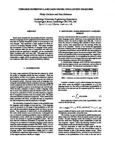
On top of the phreatic zone two zones may be distinguished: an unsaturated zone and an epikarst layer. Combined the three zones define what may be called a karst system. The concept of epikarst was introduced by (Mangin, 1975). This zone is a shallow zone of about 1 to 15 m thick and is relatively highly karstified (Klimchouk, 2004). Due to its permeability the epikarst hinders surface runoff. Infiltrated water is rapidly transferred towards the conduit network. Figure 2-1 shows the conceptual model of a karst system according to (Mangin, 1975).

Figure 2-1:

The conceptual model for a karst aquifer according to Mangin (1975).

Conduit cross-sections in the epikarst layer tend to be relatively small (Jeannin, 1996). The overall direction of conduits in the vadose zone tends to be vertical (Jeannin, 1996). In this zone where free-surface flow prevails cascade pool sections can develop (Hauns, 1999). Generally the conduits have a larger height then width due to erosion by free-surface flows.

12


Conduits in the saturated zone have elliptical forms and their overall direction is horizontal, although important vertical passages may exist (Jeannin, 1996).

2.6

Conduit-matrix flow

The existence of a high permeable conduit network within a low permeable fissured rock matrix makes a karst aquifer highly heterogeneous. The duality in permeability causes a duality in the hydrodynamics of karst aquifers (Kiraly, 1998). The conduit network is characterized by rapid, concentrated infiltration, high flow velocities and concentrated discharge at karst springs. The fissured limestone volumes are characterized by slow, diffusive infiltration, slow laminar flow and diffuse discharge. Because groundwater velocities in the conduits are relatively high, the flow in the conduits is generally turbulent (Jeannin 2001, White 2003). The main difference between laminar and turbulent flow is the role of friction. In turbulent flow friction is responsible for head losses. Under variably saturated conditions conduits can be dry, partially filled or pressurized. If conduits are partially filled the flow is a free-surface flow like the flow in a channel. An important difference between a free-surface flow and a pressurized flow is the travel speed of waves. In a free-surface flow there is empty space to accommodate for disturbances and the speed of a wave depends on the availability of this space. In pressurized flow waves travel much faster. The response to disturbances is almost instantaneously since the speed depends on the very small compressibility of water. The flow of groundwater between conduits and matrix is simply governed by gradients in hydraulic heads. After recharge events the hydraulic heads increase faster in the conduits then in the surrounding matrix. Consequently the conduits may temporarily recharge the surrounding matrix. The amount of exchanged water depends on the difference in hydraulic heads as well as on the permeability of the matrix. After the recharge event the decrease in hydraulic heads in the conduits is also faster then in the surrounding matrix and the conduits will drain the matrix until equilibrium in hydraulic heads is reached. This inversion of hydraulic heads has been tested and verified by numerical models (Kiraly 1998).

2.7

Aquifer response and hydrograph analysis

An important feature of karst systems is the concentrated discharge at springs. Typically spring hydrographs show a relatively quick response to recharge events followed by a relatively slow recession (Cornaton and Perrochet 2001). A typical spring hydrograph is shown in figure 2-2.


Saivu springSaivu

Figure 2-2:

Example of a typical spring hydrograph (Saivu spring, Milandrine, Bure, Switzerland) with a rapid response and a slow recession (data from Perrin, 2003). The other graph is a hydrograph upstream from the spring (inside the cave).

Figure 2-3:

Conceptual ideas about the factors influencing the shape of karst spring hydrographs according to Hobbs and Smart (1986).

13

14


The quick response at the spring has to be related to a quick infiltration of a certain amount of water into the conduit network. The quick infiltration means that the epikarst layer is capable of draining the infiltrated water quickly towards the conduit network. The high permeability of the conduit network allows for a subsequent quick response at the spring. The slow recession is often related to water released from storage. However, it is known that recharge and flow conditions in the karst aquifer are important as well (Hobbs and Smart, 1986; Jeannin and Sauter, 1998). Important factors influencing the flow conditions are the geometry of the conduit network and the matrix conductivity (Kovács 2003). Figure 2-3 illustrates the factors that may influence the form the hydrograph. Although the conceptual ideas about the structure and the duality of karst systems are widely accepted, the importance of the different mechanisms for storage in karst systems is disputed. According Kiraly (1975) groundwater storage in the fissured rock matrix plays a significant role. According to Mangin (1975) storage in the matrix is negligible because of the low permeability of the rock matrix and storage takes place in large voids near the water table. These voids poorly connected to the conduit system can store water simply by an increase in water level. This conceptual model is often referred to as the annex-to-drain system. Perrin (2003) and Klimchouk (2004) have pointed out that the epikarst can also store water. Moreover, the epikarst may concentrate the drainage of infiltrated water into the conduit network, decreasing the recharge of the matrix (Kiraly, 1998). Therefore the epikarst layer is not only important because of its own storage capacity, but it may also indirectly determine the storage in the matrix.

2.8

Definition of the conceptual model

The conceptual model used in this work is based on the dual porosity model. The karst aquifer is assumed to consist of high permeable conduits embedded in a continuum of low permeable fractured limestone volumes. The conduits are assumed to have circular cross-sections. The epikarst layer, if accounted for, is taken as a single continuum. Conduit flow is assumed to be turbulent under all hydraulic conditions and to be onedimensional. Furthermore the saturation in the two flow domains is a variable. The purpose of the numerical model is to simulate present day groundwater flow in karst aquifers. Therefore the conceptual model does not include any dissolution processes.

Chapter 3: The mathematical model

15

Chapter 3: The mathematical model 3.1

Introduction

In this chapter the mathematical model is introduced and discussed. The discussion contains new insights into the behavior of the underlying equations as used in the numerical model. For practical reasons simplifications are made in defining the mathematical model. It is desirable to use equations that can capture the essential physical processes with the least computational burden. As pointed out in the previous chapter the model is based on the concept of dualporosity. This means that the flow in the fractures and the porous limestone volumes can be simplified by a flow in a single porous continuum. Variably saturated flow in porous media can be described by the Richards equation. A second simplification is to assume onedimensional flow in the conduits. Turbulent conduit flow has much in common with turbulent flow in channels, except that the flow in conduits can become pressurized. One-dimensional channel flow is usually described by the Saint-Venant equations. If inertial terms can be neglected these equations can be approximated by the diffusive wave equation. These equations can be directly used to describe free-surface flows in the conduits and can be modified to describe pressurized conduit flow. The advantage of using the diffusive wave equation is its similarity with the Richard’s equation. As a consequence the discrete counterparts of the two equations can be combined in one matrix system, either by assuming continuous heads or by using exchange fluxes. This integrated approach has been used successfully for the simulation of coupled surface-subsurface flows under variable saturated conditions. It has been shown that the approach results in robust numerical schemes (VanderKwaak 1999). This chapter recalls how the Richard’s equation and diffusive wave equation can be derived, without being too exhaustive. Both equations are expressed by using the pressure head as primary variable. More details about these derivations can be found in many textbooks. For example Musy and Soutter (1991) provide more details about the derivation of the Richard’s equation. Cunge et al (1980) provide more details about the Saint-Venant equations and the diffusive wave equation. Emphasis is put on the properties of both equations since a good understanding of the equations is imperative for constructing and testing the numerical scheme. Classically the Richard’s equation and the diffusive wave equation are expressed in the form of non-linear diffusion equations. However, they can also be expressed as advection-diffusion equations. This provides a better insight into the actual physical processes as described by the equations: advection and diffusion. This insight is important because it is well known that dominantly advective processes are difficult to solve numerically. Generally the dominance

16


of the advective process is associated with steep fronts (large pressure head gradients) or with the presence of insignificant diffusion. ElKadi and Ling (1993) for example have used an advection-diffusion form of the Richard’s equation to express Péclet and Courant numbers. Makhanov and Semenov (1994) have used an advection-diffusion form of the diffusive wave equation to illustrate that a numerical scheme has to account for the advection component, especially at shallow water depths when the diffusion component becomes very small. Assuming small pressure head gradients the equations in advection-diffusion form can be simplified. These simplified equations describe the propagation of small pressure head disturbances. A study of the advection and diffusion components in these equations provides new insights. First it is shown that the advection component is non-vanishing for zero pressure head gradients. This is an important observation, since this means that numerical difficulties related to the presence of advection may even exist when steep fronts are absent. A study into the relative dominance of advection with respect to diffusion reveals that the dominance is a function of the pressure head. In free-surface flows described by the diffusive wave equation the relative dominance of advection goes to infinity if the pressure head goes to zero. This insight is more precise then the conclusions of Makhanov and Semenov (1994). At shallow water depth the strong hyperbolic nature of the diffusive wave equation is not related to a combination of vanishing diffusion with nonvanishing advection. In fact if the pressure head goes to zero, the advection component vanishes as well. Instead the strong hyperbolic behavior is related to the relative dominance of advection at shallow water depth. Furthermore it is shown that in circular conduits the relative dominance of advection also goes to infinity if the conduit is almost surcharged. For the Richard’s equation ElKadi and Ling (1993) and Diersch (2002) have pointed out that the relative dominance of advection is larger for coarse materials (characterized by a large value for the inverse air entry pressure). A similar conclusion is made in this work. Additionally it is shown that if the Van-Genuchten relationships are used then values for the pore size distribution index also influence the relative dominance of the advection component.

3.2

Conservation laws

Transport processes obey the conservation laws for mass, momentum and energy. These conservation laws are fundamental physical principles and do not depend on material properties. When applied to a fluid flow a combination of these three conservation laws results in the Euler equations. In their primitive form these laws are formulated within the Lagrangian framework. In the Lagrangian framework the conditions of a fixed mass are described as it moves. The independent variables are the initial coordinates and the time. Since the initial coordinates are constants the Lagrangian rate of change of a quantity β is given by a derivative with respect to time. This derivative is called a material derivative and is expressed as: Dβ Dt .


17

In the Eulerian framework the conditions within a fixed region of space, a so-called control volume are described. The conservation laws can be expressed in an Eulerian framework by applying Reynolds Transport Theorem (RTT) (Bear, 1972): Dβ ∂ = ρ β dV + ∫ ∇ ⋅ ( ρ β v )dV Dt ∂t ∫

(3.1)

where β is the conserved quantity, ρ β the density of β, v the velocity and V the control volume. The term in the left hand side expresses the instantaneous rate of change of β inside the control volume. The first term in the right hand side expresses the rate of change of β inside the control volume. The second term expresses the net mass flux of β through the control volume. By defining a flux function f, the RTT can also be expressed by: Dβ ∂ = ρ β dV + ∫ ∇ ⋅ f ( ρ β )dV Dt ∂t ∫

(3.2)

In words the conservation laws for mass, momentum and energy can be expressed as follows: The rate of change of mass of a system = zero The rate of change of momentum of a system = the net external force on the mass The rate of change of internal energy of a system = the work done by the external forces on the mass + the heat added to the system

Obviously the RTT is not needed to set up a mass balance equation for a control volume, but it can be useful for expressing the other two conservation laws in a control.

3.3

Flow in the matrix

3.3.1

Mass conservation

If it is assumed that density is constant and that the fluid as well as the aquifer is incompressible, then the conservation of mass applied to a control volume of matrix gives the following expression:

18


∂θ + ∇⋅q = 0 ∂t

(3.3)

where θ is the volumetric water content and q the volumetric flow rate. If the compressibility of the fluid and the aquifer are taken into account the expression for mass conservation can be written as:

 ∂s  ∂p  Ss s + ε  + ∇ ⋅q = 0 ∂p  ∂t 

(3.4)

where p is the pressure head, Ss is specific storage coefficient, s the saturation and ε the porosity of the aquifer. The specific storage coefficient can be expressed by (Bear, 1972):

Ss = ρ w g ( εκ w + (1 − ε ) κ a )

(3.5)

where ρ w is the density of the fluid, g the gravity, κ w the compressibility of water (4.5 · 1010 N/m2) and κ a the compressibility of the aquifer. In this work the compressibility of the fissured limestone volumes is defined as 5.0 · 10-10 N/m2. The porosity of a fissured limestone generally ranges from 0.005% to 0.5%. However, the porosity of the epikarst can be significantly higher and estimates range from 1% to 10% (Klimchouk, 2004).

3.3.2

Darcy’s law and Richards’ equation

Under saturated conditions the volumetric flow rate of ground water in porous media is governed by Darcy’s law: q = −K s ∇h

(3.6)

where Ks is the saturated hydraulic conductivity tensor and h the hydraulic head. The bulk hydraulic conductivity of fissured limestone volumes is about 10-6 m/s to 10-7 m/s (Jeannin, 1996). It may be assumed that Darcy’s law is also valid under unsaturated conditions. By combining Darcy’s law with the expression for mass conservation Richards’ equation is obtained as (Musy and Soutter, 1991):

 ∂s  ∂p = ∇ ⋅ ( kr ( s ) K s∇ ( p + z ) )  Ss s + ε  ∂p  ∂t  where kr is the relative hydraulic conductivity depending on the saturation.

(3.7)


19

The pressure head and the saturation are respectively the primary and secondary variable. Richards’ equation can also be expressed with the saturation as primary variable, but in that case it can only be applied to unsaturated flow. Constitutive relationships are needed to express kr as a function of s and to express the secondary variable (s) as a function of the primary variable (p). Commonly used are the Van Genuchten-Mualem, the exponential and Brooks-Corey model. Only the first two models are considered here. An overview of other models can be found in the HYDRUS manual (Šimůnek et al., 2005). Both models are expressed in terms of the so-called effective saturation se :

se =

s − sr ss − sr

(3.8)

where sr, ss and se are respectively the residual and maximum and effective saturation The Van Genuchten-Mualem model is given by (Musy and Soutter, 1991):

 1 + α p n  − m   se =   1 m kr =s e1 2 1- (1-s e1 m )   

if p < 0 if p ≥ 0

(3.9)

2

where α is the inverse of the air entry pressure head and n the pore size distribution index (n>1). The inverse of the air entry pressure head in fissured limestone volumes is assumed to be in the order of 100 m-1. For m the following relationship holds:

m = 1 −1 n

(3.10)

Figure 3-1 illustrates how kr, se depend on the pressure head, the pore size distribution index and the inverse of the air entry pressure head if the Van Genuchten-Mualem model is used. The exponential model is given by:

eα p if p < 0 se =  if p ≥ 0 1 kr =s e

(3.11)

20


1

1

n = 1.5 n = 2.0 n = 4.0

0.8

0.8

kr [-]

se [-]

0.6 0.4

0.4

0.2 0

Figure 3-1:

0.6

n = 1.5 n = 2.0 n = 4.0

0.2

-2

-1.5 -1 αp [-]

-0.5

0

0

-2

-1.5 -1 αp [-]

-0.5

0

The Van Genuchten-Mualem relationships.

3.4

Flow in the conduits

3.4.1

Mass conservation

Mass conservation for one-dimensional conduit flow in the s-direction is given by: ∂ ( ρ w A) ∂t

+

∂ ( ρ w vA ) ∂s

=0

(3.12)

where A is the cross-sectional area of flow. For a free-surface flow the density can be considered a constant. Then the equation for mass conservation simplifies into: W

∂p ∂Q + =0 ∂t ∂s

(3.13)

where W is equal to the top width of the free surface. For a closed-conduit flow the cross-sectional area of flow is constant with time. Moreover it is assumed that density is constant. If the fluid compressibility is taken into account the equation for mass conservation in a closed conduit flow can be written as (Cornaton and Perrochet 2001):

ρ w gAκ w

∂p ∂Q + =0 ∂t ∂s

(3.14)


3.4.2

21

Momentum conservation

To obtain an equation for momentum conservation expressions for the external forces are needed. The following forces are taken into account: gravity forces Fg, pressure forces Fp and friction forces Ff . The gravity force acting on a control volume can be expressed as: Fg = ∫ ρ w g sin α Ads

(3.15)

where α is the positive angle of the channel with the horizontal plane (the xy-plane) defined as follows:

sin α = −

dz dx 2 + dy 2 + dz 2

=−

∂z ∂s

(3.16)

If the bottom slope of the conduit S0 is relatively small then: S0 = −

dz dx + dy 2 2

= tan α ≈ sin α

(3.17)

The gravity force acting on the control volume can now be expressed by: Fg = ∫ ρ w gS0 Ads

(3.18)

The net pressure force can be expressed as follows: Fp = − ∫ ρ w g

∂p Ads ∂s

(3.19)

In uniform flow there are no net pressure forces and the friction force is in equilibrium with the gravity force: Ff = − ∫ ρ w gS0 Ads

(3.20)

The friction force acts along the wetted surface Aw of the conduit. This surface is given by: Aw = pm ds

(3.21)

22


where pm is the wetted perimeter (see figure 2.2). Suppose the average value for the friction force per unit wetted area (the shear stress) is given by τ0, then (Chow, 1959):

∫ρ

w

gS0 Ads = ∫ τ 0 pm ds

(3.22)

τ 0 = ρ w gS0 Rh

(3.23)

Thus:

where Rh is the hydraulic radius defined as: Rh =

A pm

(3.24)

However, in general the shear stresses are not uniformly distributed along the wetted surface. In non-uniform flow the shear stress is classically expressed in terms of the socalled friction slope Sf (Chow, 1959):

τ 0 = ρ w gSf Rh

(3.25)

The friction slope can be expressed in terms of head losses hf due to friction: Sf = −

∂hf ∂s

(3.26)

With the friction slope the friction force is expressed as: Ff = − ∫ ρ w gSf Ads

(3.27)

The integration of the three forces over the control volume can now be written as:

∫ρ

w

∂p   g  S0 − S f −  Ads ∂s  

(3.28)

Application of Reynolds Transport Theorem gives:

∫

∂ ( ρM A) ∂ ( ρ M vA) ∂p   ds + ∫ ds = ∫ ρ w g  S0 − Sf −  Ads ∂t ∂s ∂s  

(3.29)


23

where ρ M is the momentum density. Using the expression for the momentum density and writing the equation in differential form results in: 2 ∂ ( ρ w vA ) ∂ ( ρ w v A) ∂p   + = ρ w gA  S0 − S f −  (3.30) ∂t ∂s ∂s   By using the expression for mass conservation the expression for momentum conservation becomes (Cunge et al, 1980):

1  ∂v ∂v  ∂p  + v  = S 0 − Sf − g  ∂t ∂s  ∂s

(3.31)

It may be noted that the above equation is a Bernoulli equation for unsteady flows along a streamline (Rijn, 1990). For steady flow without friction the above equation simplifies into the classical Bernoulli equation by applying integration:

v2 + p+z =H 2g

(3.32)

where H is a constant resulting from integration called the total energy head.

3.4.3

Constitutive relationships for head losses

There are several constitutive relationships for the head losses. The general form of the relationship is based on two assumptions (Chow, 1959). Firstly the friction force is assumed to be proportional to the squared velocity. Secondly it is assumed that the component of the gravity force in the direction of flow equals the friction force. This is in generally only true for uniform flows. From the first assumption: Ff = ∫ cv 2 ρ w ds

(3.33)

where c is a constant. Since the friction force is a surface force the integral is taken over the wetted surface. Together with the second assumption this results in:

ρ w gAS 0 = cv 2 ρ w

(3.34)

1 ρ w gRh S0 c

(3.35)

Solving for v results in:

v=

24


In uniform flow the bottom slop equals the friction slope and therefore the general expression for head losses may be expressed by: Q = K c Sf

(3.36)

with Kc the conveyance factor. The conveyance factor can be expressed by several empirical formulas: 2 3

Manning-Strickler:

K c = η ARh

Chezy:

K c = CA Rh

(3.38)

Darcy-Weisbach:

Kc = A

8 gRh f

(3.39)

(3.37)

where η, f and C are friction factors. The friction factor η is known as the Manning’s roughness coefficient. It can be easily observed that the last two expressions for the conveyance factors are identical if f = 8g/C2. In this work the Manning-Strickler formula is used. The values for η in karstic conduits are assumed in the order 20m1/3/s. An overview of the applicability of the different empirical relationships for head losses in karstic conduits is given by Jeannin and Maréchal (1995).

3.4.4

Diffusive wave equation

The two conservation equations for free surface flow are known as the Saint-Venant equations. A well known simplification of the Saint-Venant equations is the diffusive wave equation. The diffusive wave equation is based on the assumption that the net force acting on the water particles is zero (DM/Dt = 0). This means that the momentum equation for a steady flow is used, in other words all the acceleration terms in the momentum equation are neglected. By making this assumption the momentum equation becomes: ∂h = − Sf ∂s

Differentiating the general equation for head losses with respect to s results in:

(3.40)


 ∂Q ∂ ∂ K = Kc S f =  c S f   ∂s ∂s ∂s  S f  

(

)

25

(3.41)

Combining the last expression with the momentum equation gives:

∂Q ∂ =−  ∂s ∂s  

∂h   ∂h ∂s ∂s  Kc

(3.42)

Combined with mass conservation this gives the diffusive wave approximation:

C

∂p ∂  =  ∂t ∂s  

∂h   ∂h ∂s ∂s  Kc

(3.43)

The evaluation of the terms C and Kc depends on conduit geometry and the type of flow. For closed conduit flow these terms are independent of pressure head. For free surface flow the terms are non-linear and depend on the pressure head. For the capacitive term:

W C=  ρ w gAκ w

for free-surface flow for closed conduit flow

(3.44)

The conveyance factor is a function of the cross-sectional area of flow and the wetted perimeter. So to evaluate the terms C and Kc expressions for Wp, A and pw are needed. In the following these expressions are given for two conduit geometries: circular and rectangular. They follow from geometry (see figure 3-2). For saturated conduit flow in a circular conduit with radius r:

W =0 A = π r2 pm = 2π r For free surface flow in a circular conduit with radius r:

(3.45)

26


W = 2p

2r −1 p

p 2r  A = r 2 arccos 1 −  + p ( p − r ) −1 r p 

(3.46)

p  pm = 2r arccos 1 −   r

W

B

H

p

r θ

pm

pm Figure 3-2:

Geometry of circular and rectangular conduits

3

3 *

W

* *

pm Rh * Kc

*

*

pm Rh *

2

Kc

*

*

1.5 1

*

1

*

*

*

*

1.5

A

*

*

2

*

2.5

*

A

*

W , A , pm , Rh and Kc [-]

2.5

*

W , A , pm , Rh and Kc [-]

W

0.5 0 0

Figure 3-3:

0.5

1 p/B [-]

1.5

2

0.5 0 0

0.5

1 p/r [-]

1.5

2

Normalised hydraulic parameters as a function of pressure head. For a rectangular channel the parameters are normalized with respect to the values at p = B. For a circular conduit the parameters are normalized with respect to the values at p = r.


27

Alternatively (Chow, 1959):

W = 2r sin A=

θ 2

2

r (θ − sin θ ) 2 pm = rθ

(3.47)

where:  

θ = 2 arccos 1 −

p  r

(3.48)

For saturated conduit flow in a rectangular conduit with width B and height H: A = BH pm = 2 B + 2 H

(3.49)

For free surface flow in a rectangular conduit with width B:

W =B A = Bp pm = B + 2 p

(3.50)

Figure 3-3 shows the cross-sectional area of flow, the wetted perimeter, the hydraulic radius and the conveyance factor as functions of pressure head for a rectangular channel and a circular conduit. For a circular conduit section the hydraulic radius and the conveyance factor have a maximum before the conduit is full. This means that above a certain water depth the positive effect of increased cross-sectional area on the conveyance factor is less then the negative effect of increased friction with the side walls. The water depth with the maximum conveyance is also the water depth with the maximum volumetric flow rate for a freesurface flow. The maximum in hydraulic radius corresponds to p ≈ 1.63r . The maximum in conveyance corresponds to p ≈ 1.88r . If the bottom slope is known the plot of the conveyance factor as a function of p can be used to obtain the rating curve for steady flows since Q = K c S 0 . A rating curve is a plot of the discharge versus the water depth.

28

3.4.5


Alternatives for the diffusive wave equation

Another well known simplification of the Saint-Venant equations is the kinematic wave equation. It is based on the assumption that the pressure head gradient is small compared to the bottom slope. This means that this equation cannot be used for pressurized conduit flow. Nonetheless, it is a useful equation to consider. By neglecting the pressure head gradient the momentum equation for a steady and uniform flow is obtained: S0 = S f

(3.51)

From the general equation for head losses it follows that: ∂Q ∂K c = ∂p ∂p

S0

(3.52)

The mass balance equation can also be written as: W

∂p ∂Q ∂p + =0 ∂t ∂p ∂s

(3.53)

Combining the last two equations gives the kinematic wave equation:

∂p  1 ∂K c + ∂t  Wp ∂p

 ∂p S0  =0  ∂s 

(3.54)

If a pressurized flow in a pipe is assumed to be laminar Poiseuille’s law for flow in a pipe can be used. It relates the volumetric flow rate to the hydraulic gradient:

ρ w gπ R 4 ∂h Q=− 8µ ∂s

(3.55)

where µ is the dynamic viscosity.

3.5

Properties of the flow equations

3.5.1

Similarity of the flow equations

The equations for matrix flow and conduit flow can be captured by a single expression:


C ( p)

∂p = ∇ ⋅ ( Kα ( p ) ∇ ( p + z )) ∂t

29

(3.56)

where the capacitive term C(p) and the equivalent conductivity term Kα(p) are non-linear terms depending on the pressure head. The expressions for both terms depend on the type of flow:

W ( p )  C ( p ) =  ρ w gAκ w  S s + ε ∂s ∂p  s  K c ( p ) / ∂h ∂s Kα ( p ) =  kr ( p ) K s

for free-surface flow for closed conduit flow for matrix flow

(3.57)

for conduit flow for matrix flow

Equation (3.54) may also be written as: C

∂h = ∇ ⋅ ( K α ∇h ) ∂t

(3.58)

with h = p + z. This equation is referred to in the following as the general flow equation The general flow equation is a non-linear diffusion equation and it can be classified as a PDE of parabolic type. To solve this kind of PDE initial conditions as well as boundary conditions need to be specified. Since the PDE is of parabolic type the boundary conditions need to be specified on the entire boundary of the solution domain. Under saturated conditions the equation for matrix flow is linear. Although the conveyance factor is linear for saturated conduit flow, the equivalent conductivity term is not since it depends on the hydraulic gradient. Hence the equation for conduit flow is always non-linear.

3.5.2

The flow equations in terms of advection and diffusion

The actual processes described by the flow equations are more evident if the equations are expanded in advection and diffusion terms. The particular properties of the general flow equation may be illustrated by making a comparison with the following 1D non-linear diffusion equation for a primary variable u with D being the non-linear diffusion coefficient: ∂u ∂  ∂u  −  D (s)  = 0 ∂t ∂s  ∂s 

(3.59)

30


In the following this equation is referred to as an ordinary non-linear diffusion equation. This equation can be written as an advection-diffusion equation as follows: ∂u ∂D ∂u ∂ 2u − −D 2 =0 ∂t ∂s ∂s ∂s

(3.60)

It can be noted that this can also be written as: ∂u ∂D  ∂u  ∂ 2u − − =0 D   ∂t ∂u  ∂s  ∂s 2 2

(3.61)

This expression reveals that the advection component goes to zero if the gradient of u vanishes. If the gradients in u vanish, then the above equation degenerates into a linear diffusion equation. In the case of steep fronts the gradient of u and the advection component are relatively large Expanding the general 1D flow equation as an advection-diffusion equation gives:

∂p 1 ∂K α ∂h K α ∂ 2 h − − =0 ∂t C ∂s ∂s C ∂s 2

(3.62)

The fundamental difference with the ordinary non-linear diffusion equation is that h is another kind of variable then u. The variable h is the sum of the variable p and the constant z. Substituting h = p + z :

∂p 1 ∂K α  ∂p ∂z  K α  ∂ 2 p ∂ 2 z  − +  =0  + − ∂t C ∂s  ∂s ∂s  C  ∂s 2 ∂s 2 

(3.63)

Or:

∂p 1 ∂K α − ∂t C ∂p

2 2  ∂p ∂z  ∂p K α  ∂ p ∂ z  + − +  2 =0   ∂s 2   ∂s ∂s  ∂s C  ∂s

(3.64)

This equation illustrates that if ∂K α ∂p ≠ 0 and if ∂z ∂s ≠ 0 then the advection coefficient has a certain value if the pressure head gradient is negligible due to gravity effects. This is an important difference with the ordinary non-linear diffusion equation. One dimensional matrix flow in the z-direction can be described by the following advection-diffusion equation:


2 ∂p K s ∂kr ( s )   ∂p  ∂p  K s ∂2 p − kr ( s ) 2 = 0   +  − ∂t C ∂p   ∂z  ∂z  C ∂z

31

(3.65)

For conduit flow in a straight sloping channel ( ∂ 2 z ∂s 2 ≠ 0 ) the term ∂K α ∂p is expanded as:

∂K α Kc ∂  K  1 ∂K c ∂s ∂ 2 p =  c = + 2 ∂p ∂p  S f  S f ∂p 2 S f S f ∂p ∂s  

(3.66)

Combining equation 3.61 and equation 3.63 gives the advection diffusion equation describing conduit flow is: 2 Kc ∂2 p ∂p 1 ∂K c   ∂p  ∂z ∂p  − =0   + − ∂t C S f ∂p   ∂s  ∂s ∂s  2C S f ∂s 2

(3.67)

It is noted that the advection-diffusion form of the diffusive wave equation can also be written with Q as primary variable (Cunge et al., 1980). The expanded equations give more insight into the described physical processes: advection and diffusion of disturbances in pressure head. Under fully saturated conditions the advection coefficients are zero and conduit flow and matrix flow are governed by diffusion alone. Since the compressibility of water has a very small value it can be observed that disturbances in closed conduits travel very fast by means of diffusion. Under variably saturated conditions the flow is described by advection plus diffusion. In variably saturated matrix flow disturbances in terms of pressure head coincide with disturbances in saturation. In a free-surface flow disturbances in terms of pressure head simply coincide with disturbances in water depth.

3.5.3

Wave propagation in free-surface flows

The kinematic wave equation is an advection equation. For this type of PDE no boundary conditions are needed on the outflow boundaries. It can be observed that this equation describes a wave in terms of pressure head with a certain speed, which is called the kinematic wave velocity vk:

vk =

1 ∂Q 1 ∂K c = Wp ∂p Wp ∂p

S0

This expression is also known as the Kleitz-Seddon law (Chow, 1959).

(3.68)

32


Kinematic waves travel without diffusing and travel only downstream. Consequently the kinematic wave equation can not describe back water effects (disturbances traveling upstream). The advection-diffusion form of the diffusive wave equation is now written in the following form: ∂p ∂p ∂2 p + vw − Dw 2 = 0 ∂t ∂s ∂s

(3.69)

where cw [m/s] and Dw [m2/s] are respectively the advection and diffusion coefficient for a wave in terms of pressure head. The coefficients are given by (see equation 3.64): 1 ∂K c Sf C ∂p Kc Dw = 2C S f

vw =

(3.70)

The ratio expressing the relative dominance of advection relatively to diffusion is given by: vw 2 S f ∂K c = Dw K c ∂p

(3.71)

If the pressure head gradients are negligible with respect to the bottom slope (only possible for a free-surface flow) these coefficients may be approximated as:

1 ∂K c W ∂p Kc Dw = 2W S 0

vw = vk =

 S0  ∂z  ∂p ≪  if ∂s  ∂s 

(3.72)

Thus under certain conditions the diffusive wave equation describes a wave with a velocity equal to the kinematic wave velocity. Obviously the advection coefficient is proportional to η S0 . Similarly the diffusion coefficient is proportional toη S0 . The coefficients also depend on the pressure head and the conduit geometry. In certain cases the coefficients terms can be easily evaluated. For a relatively wide rectangular channel (relative to the water depth) the wetted perimeter is approximately equal to the top width of the channel (B). In that case simple


33

expressions can be derived for the advection coefficient, the diffusion coefficient and their ratio: 2 p3  3  5  η  Dw = p 3  if B ≫ p 2 S0  vw 5 S 0   = Dw 6 p 

vw =

5η S0

(3.73)

This shows that in a wide rectangular channel the advection and diffusion increase for larger water depth. Although both coefficients go to zero the pressure head goes to zero, their ratio goes to infinity. For a relatively narrow rectangular channel (relative to the water depth) the wetted perimeter is approximately equal to two times the water depth. In that case:  S0   2 5 −  if p ≫ B 3 3 ηB 2 p  Dw =  S0  2 3

vw = η B 2

−

2 3

(3.74)

This shows that in a narrow channel with relatively high water levels the advection and diffusion become larger for larger width. Moreover, the wave velocity is independent of pressure head and the diffusion scales linearly with pressure head. Figure 3-4 shows the plots of the advection and diffusion coefficients and their ratio as a function of pressure head for a rectangular channel and a circular conduit. For rectangular channels it can be observed that when the ratio p/B becomes large enough that the velocity becomes approximately constant and that the diffusion becomes a linear function of pressure head. If the pressure head goes to infinity, the ratio goes to zero. If the pressure head goes to zero the coefficients go to zero. However, the ratio goes to infinity. This means that the relative importance of advection with respect to diffusion is very large for small water depths. In circular conduits the situation is more complicated. The behavior of the coefficients if the pressure head goes to zero is identical as found for rectangular channels: both coefficients go to zero. Again the ratio goes to infinity. As can be observed from figure 3-3 the conveyance factor decreases as a function of pressure head if the pressure head is close to the top of the conduit (if the pressure head is larger then about 94% of the diameter). This means that if the free surface is close to the top of the conduit the wave

34


velocity becomes negative as indicated in figure 3-4. In fact, in the limit as the pressure head goes to the value equal to the diameter of the conduit, the advection coefficient becomes infinitely negative. With a negative wave velocity the downstream propagation of disturbances in pressure head is hindered. To explain this, a straight sloping conduit with radius r is considered. Suppose the initial pressure head profile pold is constant and below 94% of the conduit’s diameter. If from t = 0 s the pressure head at the inlet is increased to pnew then after a certain time a new steady state is obtained with a constant pressure head profile given by pnew. The disturbance has been advected (and diffused) over the full length of the conduit. However if pold was above 94% of the diameter, a new steady state is not defined by a constant pressure head. Instead, the new steady state is characterized by a decreasing water depth in a downstream direction, because of negative advection. The strong advective nature of the diffusive wave equation at shallow water depth has also been discussed by Makhanov and Semenov (1994). They considered the role of the advection and diffusion terms for a vanishing water depth as well. However, they concluded that the diffusion term vanishes while the advection term does not. Here is has been shown that the advection term also vanishes if p goes to zero. But the ratio of advection and diffusion that goes to infinity when p goes to zero and this invokes the strong advective nature of the equation at shallow water depths.

*

vw Dw * * (vw/Dw)

4

*

vw , Dw and (vw/Dw) [-]

4 3

3 2

*

2

1

*

*

*

5

*

vw Dw * * (vw/Dw)

*

vw , Dw and (vw/Dw) [-]

5

1 0 0

Figure 3-4:

0.5

1 p/B [-]

1.5

2

0 -1 0

0.5

1 p/r [-]

1.5

2

Advection and diffusion coefficients for free-surface flows and their ratio as a function of pressure head. For a rectangular channel the coefficients and their ratio are normalized with respect to the values at p = B. For circular conduits the coefficients and their ratio are normalized with respect to the values at p = r.


3.5.4

35

Propagation of pressure head contours in unsaturated vertical matrix flow

The advection-diffusion form of the diffusive wave equation is now written in the following form: ∂p ∂p ∂2 p + vω − Dω 2 = 0 ∂t ∂z ∂z

(3.75)

where vω [m/s] and Dω [m2/s] are respectively the advection and diffusion coefficient for a wave in terms of pressure head. Assuming zero specific storage and taking z positive in a downward direction the advection and diffusion coefficients are given by: vω =

K s  ∂kr ( s ) ∂kr ( s )  +   ε ∂s ∂p  ∂z ∂p  Dω =

Ks kr ( s )

(3.76)

ε ∂s ∂p

The advection coefficient can also be expressed as: vω =

K s ∂kr ( s )  ∂p  +1 ε ∂s ∂p ∂p  ∂z 

(3.77)

Again it may be assumed that disturbances in pressure head are relatively small. In that case the advection coefficient can be approximated as: vω =

K s ∂kr ( s ) ε ∂s ∂p ∂p

if

∂p ≪1 ∂z

(3.78)

Both coefficients are proportional to K s ε . To illustrate how the coefficients depend on the pressure head and the Van Genuchten parameters, a dimensionless pressure head p* is defined: p* = α p

(3.79)

Using the dimensionless pressure head the following dimensionless variables are defined:

36


1 ∂kr ∂s ∂p* ∂p* kr λ* = ∂s ∂p*

κ* =

µ* =

(3.80)

1 ∂kr kr ∂p*

Then the coefficients and their ration for small disturbances are given by: vω =

Ks

κ*

Dω =

Ks

λ*

ε

εα

(3.81)

cω = αµ * Dω

This illustrates that large values for the air entry pressure result in a small diffusion coefficients and a large relative dominance of advection. If the exponential model is used then:

κ* =1 λ * = kr µ* =

(3.82)

1 kr

Thus with the exponential model the advection is constant and the diffusion depends on the saturation. If the saturation is small then the diffusion is small and consequently the relative importance of advection is large. The dimensionless parameters can also be evaluated with the Van GenuchtenMualem model. These expressions are relatively complicated and depend on the pressure head and the pore-size distribution n. Figure 3-5 gives an idea how the dimensionless parameters κ*, λ* and µ* depend on the dimensionless pressure head and the pore size distribution index. The figure illustrates that the advection coefficient has a distinct maximum if n ≥ 2 . If n > 2 then the relative dominance of advection goes to zero if the pressure head goes to zero. If n < 2 then the relative dominance of the advection goes to infinity if the pressure head goes to zero.

κ*,λ* and µ*

κ*,λ* and µ*

κ*,λ* and µ*


10 9 8 7 6 n = 1.5 5 4 3 2 1 0 -2.5

10 9 8 7 6 n = 2.0 5 4 3 2 1 0 -2.5

10 9 8 7 6 n = 4.0 5 4 3 2 1 0 -2.5

Figure 3-5:

37

κ λ* * µ *

-2

-1.5

αp [-]

-1

-0.5

0

-1

-0.5

0

-1

-0.5

0

κ * λ * µ *

-2

-1.5

αp [-]

κ * λ * µ *

-2

-1.5

αp [-]

The dimensionless parameters as a function of dimensionless pressure head for different pore size distribution indices.

38

3.6


Summary

The Richard’s equation and the diffusive wave equation can be captured by a single expression, referred to in this work as the general flow equation: C

∂h = ∇ ⋅ ( K α ∇h ) ∂t

(3.83)

where h is the hydraulic head, C the non-linear capacitive term and Kα the non-linear equivalent conductivity. This equation is a non-linear diffusion equation and consequently can also be expressed in terms of advection and diffusion. Since the hydraulic head is the sum of a variable pressure head and a constant elevation head it can be shown that the general flow equation invokes an advection component that is non-vanishing for zero gradients in the pressure head. This work provides new insides into the relative dominance of this non-vanishing advection component (with respect to diffusion) as a function of the pressure head. For free-surface flows described by the diffusive wave equation the dominance goes to infinity when the water depth goes to zero. In circular conduit flow the dominance also goes to infinity if the conduit is almost surcharged. For flow described by the Richard’s equation the dominance is largest near saturation. The dominance can be particularly large for coarse materials characterized by a large value for the inverse air entry pressure. If the van Genuchten relationships are used then the dominance of advection also depends on the value for the pore size distribution index. The advection and diffusion coefficients evaluated for zero gradients in pressure head apply to the propagation of very small disturbances in pressure head. Insight into the propagation of such disturbances is important from a numerical point of view. Very small disturbances in pressure head may be generated by numerical errors. If advection is relatively dominant such disturbances may not be smoothed out and oscillations may be generated.

Chapter 4: The numerical model

39

Chapter 4: The numerical model 4.1

Introduction

The model is based on a new combination of existing well known and less known numerical techniques. These techniques are recalled in this chapter. For some numerical techniques additional new insights are provided. In general a numerical scheme is based on the discretisation of equations in space and time. The most common methods in hydrogeology to translate a mathematical model into a numerical scheme are the finite difference method and the finite element method. In essence these methods establish functions on discrete points in the time-space domain and they result in matrix systems to be solved. The numerical scheme presented in this chapter is based on the Galerkin finite element method. Two types of elements are used to represent the structure of the karst aquifers: linear discrete elements for the conduits and linear tetrahedral elements for the matrix. The discretisation of the matrix into tetrahedral elements offers great flexibility for fitting in a conduit network. The choice of the finite element method is mainly based on this flexibility. To solve the non-linear flow equations a Picard iteration scheme is implemented. This method has a lower order of convergence then the more sophisticated NewtonRaphson method. However, the convergence rate of the iteration method is only a secondary factor influencing the speed of the numerical scheme. The primary factor determining the speed of simulations is the size of allowable time steps. It is desirable to use time steps as large as possible as to decrease the amount of calculations. Instead of focusing on a sophisticated algorithm for adaptive time stepping this work puts emphasis on increasing the numerical stability as to decrease restrictions on the time stepping. A second reason to consider the numerical stability in detail is that numerical instability can result in spurious simulation results. As pointed out by Forsyth and Kropinski (1997) upstream weighting is needed to obtain monotone schemes for non-linear parabolic problems. Without the upstream weighting of equivalent conductivities the schemes for conduit and matrix flow generate overshooting and spurious minima and maxima at material discontinuities. Their upstream weighting procedure points for evaluating equivalent conductivities are located on element edges. However, as discussed by Forsyth and Kropinski (1997) upstream weighting only guarantees monotonicity if the stiffness matrix has non-positive off-diagonal entries. This is of particular concern, since it is known that this condition is hard to fulfill for tetrahedral elements. VanderKwaak (1999) has also discussed the problem about the sign patterns of stiffness matrices. An alternative upstream weighting procedure is also considered. This procedure has been proposed by Diersch and Perrochet (1999). In this procedure the evaluation points in the element as used for classical central weighting are moved in an

40


upstream direction, such that the points for evaluating equivalent conductivities are located on element boundaries. Furthermore a special positivity preserving scheme as developed by Makhanov and Semenov (1994) is needed to avoid undecaying oscillations in the simulation of freesurface flows with shallow water depths. This works provides new arguments for using their special positivity preserving scheme. It is shown that their scheme is highly efficient for simulating free-surface flows near steady state. In order to discuss upstream weighting and the special positivity preserving scheme as well as other numerical techniques to enhance numerical stability such as implicit time marching and mass-lumping, it is useful to consider the concept of so-called monotone schemes. This concept is particular useful for studying the stability of non-linear schemes. This is because the Fourier analysis cannot be applied in a straightforward manner to nonlinear schemes. The coupling of conduit-matrix flow, the definition of proper boundary conditions at springs, the treatment of flow transitions and the treatment of the wetting-drying processes in the conduits are discussed at the end of this chapter.

4.2

The non-linear matrix system

Applying the Galerkin finite element procedure and a first order finite difference for the time derivative to the general flow equation results in the following non-linear matrix system: 1  t +∆t  1   t t +∆t t ε G + ∆t B  p =  ∆t B + ( ε − 1) G  p − [G ] z + ε Q + (1 − ε ) Q

(4.1)

where G and B are respectively the global conductance and capacitance matrix, p the nodal pressure head vector, Q the vector representing the fluxes on the boundary nodes ∆t the time step size and ε a time weighting parameter ( 0 ≤ ε ≤ 1 ). The time marching method is said to be explicit if ε = 0 and implicit if ε = 1 . By using Taylor series it can be verified that explicit and implicit time marching are first order accurate. The Crank Nicholson scheme corresponds to ε = 0.5 and is second order accurate. Implicit time marching enhances numerical stability. Therefore in this work only implicit time marching is considered. The non-linear matrix system then reads: 1  t +∆t  1  t  t +∆t G + ∆t B  p =  ∆t B  p − [ G ] z + Q

(4.2)


41

The global matrices G and B are also respectively known as the mass matrix and the stiffness matrix. The global matrices are generally assembled from the elemental matrices Be and Ge:

Be =

∫ NN CN T

T

d Ωe

Ωe

Ge =

T T e ∫ ∇NN K α ∇N d Ω

(4.3)

Ωe

where Ωe represents the element domain, N the vector containing the shape functions, C the nodal capacitance vector and Kα the nodal equivalent conductivity vector. The element mass matrix above is a consistent mass matrix. A well-known alternative is the masslumped mass matrix. When mass-lumping is used the element mass matrix is defined by:

(B )

e ij ML

=

∫ N Cδ i

i ij

d Ωe

(4.4)

Ωe

Within an element with n nodes the shape functions are defined such that:

1 Nk =  0 n

∑N i =1

i

at node k at all other nodes

(4.5)

=1

Expressions for the shape functions of linear 1D elements and tetrahedral elements and analytical integration formulas (needed to evaluate the expressions for the elemental matrices) can be found in standard textbooks about the finite element method (Zienkiewicz, 1971). In the presented numerical code analytical integration is used.

4.3

The linear matrix system

In general an iterative method is used to account for the non-linear coefficients C and Kα. The Picard iteration method is the simplest iterative method for solving a set of nonlinear discrete equations. Its drawback is its first order convergence rate. An alternative is the Newton-Raphson method with a higher rate of convergence. However, the computational work per iteration is generally higher (Mehl, 2006). Another drawback of the Newton-Raphson method is that it is more sensitive to the initial guessed solution then the Picard method (Paniconi and Putti, 1994). As an alternative for using iteration methods

42


Kavetski et al. (2002) have studied non-iterative formulations for numerical solving the non-linear Richards equation. T he overall performance of a numerical code in terms of CPU-time is, however, not only determined by the iteration method. It can be argued that the overall performance is more influenced by numerical stability. Unstable schemes generate oscillations that need to be controlled by restrictions on the time stepping. To develop cost effective numerical schemes it is important to have as few restrictions on the time stepping as possible. In this work the numerical stability is taken as a priority and the iteration method of choice is the one that is the easiest to implement: the Picard method. Also under-relaxation, the wellknown technique to improve the convergence of the Picard method (Cooley, 1983; Durbin and Delemos, 2007), is not considered. The key idea of the Picard iteration scheme is to reevaluate the non-linear coefficients with the solution of the last Picard iteration and to solve the resulting linear matrix system. The process is repeated until a certain convergence criterion is satisfied. For the first iteration the dependent coefficients can be evaluated with the solution of the previous timestep. The linear matrix system to be solved at each iteration can be expressed as: 1   G + ∆t B 

t +∆t , n

1  p t +∆t , n +1 =  B   ∆t 

t +∆t , n

pt − [G ]

t +∆t , n

z + Q t +∆t

(4.6)

where n denotes the iteration level. Two types of convergence criteria are implemented: an absolute and a relative error criterion. With δ being a certain tolerance the absolute error criterion to be satisfied reads: pin +1 − pin ≤ δ

(4.7)

The relative error criterion is defined as: pin +1 − pin pin +1

4.4

≤δ

(4.8)

The modified Picard approximation

It is known that the discretised form of the head-based Richards equation is prone to mass balance errors. Schemes using the saturation-based Richards equation have a far better performance. However, the Richard’s equation with the saturation as primary variable is restricted to unsaturated conditions. Advanced schemes have been developed that use saturation-based Richards equation under unsaturated conditions and the headbased Richards equation under saturated conditions by means of the so-called primary


43

variable switching technique (Diersch and Perrochet, 1999; Forsyth et al., 1995). On the other hand numerical solutions of the head-based Richard’s equation may be improved by using the so-called mixed-form of the Richards equation (Celia et al., 1990): ∂θ = ∇ ⋅ ( K (θ ) ∇ ( p + z ) ) ∂t

(4.9)

The Picard iteration scheme then takes the following form: t +∆t , n ( Bɶ 

θt +∆t ,n +1 − θt ) ∆t

= − [G ]

t +∆t , n

(pt +∆t , n +1 + z )

(4.10)

with:

Bɶ e =

∫ NN

T

d Ωe

(4.11)

Ωe

The modified Picard approximation introduced by (Celia et al., 1990) is based on the expansion of θ t +∆t , n +1 in a truncated Taylor series:

θ

t +∆t , n +1

≈θ

t +∆t , n

 ∂θ  +   ∂p 

t +∆t , n

(p

t +∆t , n +1

− p t +∆t ,n )

(4.12)

The modified Picard approximation is then found as:

[B]

t +∆t , n

(p

t +∆t , n +1

− p t +∆t ,n )

= − Bɶ 

∆t

t +∆t , n

(θ

t +∆t , n

− θt )

∆t

− [G ]

t +∆t , n

(pt +∆t ,n +1 + z )

(4.13)

The modified Picard approximation can also be applied to the diffusive wave equation. For a conduit: W

∂p ∂A = ∂t ∂t

(4.14)

The Taylor series expansion gives: t +∆t , n +1

A

t +∆t , n

≈A

 ∂A  +   ∂p 

t +∆t , n

(p

t +∆t , n +1

− p t +∆t ,n )

(4.15)

44


The modified Picard approximation is written as:

[B]

t +∆t , n

(p

t +∆t , n +1

− pt +∆t ,n )

∆t

t +∆t , n ( = − Bɶ 

A t +∆t ,n − A t ) ∆t

− [G ]

t +∆t , n

(pt +∆t ,n +1 + z )

(4.16)

In the numerical scheme the modified Picard approximation is implemented as an option. In this thesis mass balance problems resulting from using the head-based form of the Richard’s equation are not considered. It is, however, important to mention that these problems exist.

4.5

Spatial discretisation

4.5.1

Discrete-continuum approach

To represent the structure of a karst aquifer the discrete continuum approach is used. This approach is a simple combination of a continuum approach and a discrete approach. Within the context of spatial discretisation this means that discrete elements are nested within the element mesh defining the continuum. The approach leads to common nodes: nodes that belong to discrete as well as higher dimensional elements. The discrete continuum approach has been used for several coupled flow problems: coupled conduitmatrix flow (Bauer et al., 2005; Cornaton and Perrochet, 2002; Kiraly, 1985; Liedl et al., 2003), surface-subsurface flow (VanderKwaak, 1999) and rock-fracture flow (Therrien and Sudicky, 1996). A tetrahedral mesh offers the greatest flexibility for embedding conduit networks with relative complex geometries. Instead of trying to fit discrete features into an existing tetrahedral mesh, it is highly desirable to constrain the tetrahedralization to a pre-defined conduit network. This possibility is offered by TetGen, a tetrahedral mesh generator developed by Si (2006). The tetrahedral meshes generated with TetGen are Delaunay or constrained Delaunay.

4.6

Numerical stability

Since the general flow equation is non-linear and inhibits hyperbolic properties it is a difficult equation to solve numerically. The main difficulty is to develop a numerical scheme with sufficient numerical stability. If the numerical scheme is unstable numerical errors may be amplified. This leads to spurious oscillations. In order to maintain convergence these oscillations need to be controlled. On a fixed mesh the only way to control oscillations is to decrease the size of the time step. As such numerical stability is important for two reasons: to avoid spurious oscillations and to relax the restrictions on time stepping.


45

For unsaturated subsurface flows Forsyth and Kropinski (1997) have demonstrated that monotonicity is a sufficient condition to prevent the generation of local minima and maxima. They showed that monotonicity can be ensured if upstream weighting is used and if certain conditions on the geometry of the mesh are met. Makhanov and Semenov (1994) have pointed out that a numerical scheme for the diffusive wave equation has to preserve positive values for the pressure heads in order to avoid numerical instability. They developed a finite difference scheme with a special iteration algorithm for solving the non-linear equation. Their scheme also uses upstream weighting, but it is their special iteration algorithm that guarantees positivity. In the following some useful methods for analyzing numerical stability are introduced. Consequently these methods are applied to two problems: a 1D linear advection diffusion problem and a 1D non-linear diffusion equation. These applications show why and when implicit time marching, mass-lumping, upstream weighting and upwinding are needed for numerical stability. The solutions of the continuous equations do not contain oscillations. Therefore a natural requirement for a numerical scheme is that the properties of the continuous equations are well reflected by their discrete counterparts. This requirement is fulfilled by so-called monotone schemes. In the following n denotes either the time level or the iteration level. The definition of a monotone scheme (for a variable u) is (LeVeque, 1992): Suppose u and uɶ are two distinct evolutions. A scheme is monotone if for all time levels (or iteration levels) n and for all nodes i: uin ≥ uɶin ⇒ uin +1 ≥ uɶin +1 This definition means that uin +1 is a monotone function of its arguments (the values of u at levels n and n+1 of which uin +1 is a function). If the m arguments of uin +1 are denoted as ⌣ ⌣ u1 ,...., um then the scheme may be written in implicit form as:

⌣ ⌣ gi ( uin +1 , u1 ,...., um ) = 0

(4.17)

⌣ If uin +1 is a monotone function of its arguments then for each argument uk (1 ≤ k ≤ m): ∂uin +1 ⌣ ≥0 ∂uk

(4.18)

It can be illustrated that monotone schemes do not create or amplify minima and maxima and as such must be free of oscillations (Forsysth and Kropinski, 1997). The scheme for variable u is assumed to be defined such that if all the arguments have the same ⌣ value ( uk = constant = u * ) then:

46


gi ( uin +1 , u * ,......, u * ) = 0

(4.19)

{

}

has a unique solution uin +1 = u * . The set of arguments is denoted by arg ( uin +1 ) and the maximum argument is given by u max = max arg ( uin +1 ) . Since uin +1 is a monotone function of its arguments the upper bound for uin +1 is obtained if:

{

}

u = constant = u max

(4.20)

These arguments give the unique solution: uin +1 = u max . If some of the arguments have a lower value than umax then it follows that uin +1 < u max (since uin +1 is a monotone function of its arguments). Therefore in general given u max = max arg ( uin +1 ) :

{

}

{

}

{

}

uin +1 ≤ max arg ( uin +1 )

{

(4.21)

}

Similarly given u min = min arg ( uin +1 ) : uin +1 ≥ min arg ( uin +1 )

In summary, if a scheme is monotone then for all nodes i:

{

}

{

}

min arg ( uin +1 ) ≤ uin +1 ≤ max arg ( uin +1 )

(4.22)

This means that a monotone scheme cannot create or amplify minima and maxima and as such must be free of oscillations. A less strict requirement for numerical schemes is that it is monotonicity preserving. The definition of a monotonicity preserving scheme is (LeVeque 1992): A scheme is monotonicity preserving if: ui0 ≥ ui0+1 ⇒ uin ≥ uin+1

ui0 ≤ ui0+1

⇒ uin ≤ uin+1 for all i and n

This means that if the initial values are a monotone function of i, then all the following solutions are monotone functions of i as well. If a scheme preserves monotonicity then it obeys the discrete maximum principle. The discrete maximum principle is the discrete equivalent for the continuous maximum principle. The maximum principle states that in the absence of sources and sinks the minimum and maximum values are located at the


47

boundaries (Borisov and Sorek, 2004). If a scheme is monotone then it is monotonicity preserving (LeVeque 1992). A scheme is said to preserve positivity if positive initial conditions and positive boundary conditions exclude the possibility of generating negative values. This follows directly from monotonicity: if the boundary conditions are positive then the minima are also positive. The necessary condition for a scheme to preserve positivity for u is: A scheme preserves positivity if: uin ≥ 0 ⇒ uin +1 ≥ 0 for all i and n

In the previous chapter it has been shown that the general flow equation can be also be expressed as an advection-diffusion equation with non-linear advection and diffusion coefficients. Therefore it is useful to consider the 1D linear advection-diffusion equation. This equation is a classical example of a linear problem that can give rise to numerical instability. The general form of the 1D linear advection-diffusion equation can be written as: ∂c ∂c ∂ 2c +v −D 2 =0 ∂t ∂s ∂s

(4.23)

where c is the concentration, v is a constant velocity and D a constant diffusion coefficient. A finite difference scheme in semi-discrete form for the advection-diffusion equation can be written as: cit +∆t − cit v D + ( ci +1 − ci −1 ) − 2 ( ci −1 − 2ci + ci +1 ) = 0 ∆t 2 ∆s ∆s

(4.24)

where the first-order derivative is approximated by a central difference. This scheme is similar to a finite element scheme if lumped mass matrices are used. In fully discrete form this can be written as: t t +∆t gi ( cit−+∆ , cit++∆1 t , cit−1 , cit , cit+1 ) = 1 , ci

 D v  t +∆t  ∆s ε 2 D  t +∆t  D v  t +∆t −  ci −1 +  +  ci + ε  − +  ci +1 + ∆s   ∆s 2   ∆t  ∆s 2   ∆s (1 − ε ) 2 D  t D v  D v t (1 − ε )  − −  cit−1 +  − +  ci + (1 − ε )  − +  ci +1 ∆s  ∆s 2   ∆s 2   ∆t  =

ε −

0

(4.25)

48


A first step in considering the stability of the scheme using the concept of monotone schemes is to prove that gi ( c* , c* , cit++∆1 t , c* , c* , c* ) = 0 has the unique solution cin +1 = c* . It can be verified that cin +1 = c* is indeed a unique solution. Using the implicit function theorem reveals that cit +∆t is a monotone function of the upstream arguments cit +∆t and cit +∆t . For the other arguments certain conditions have to be fulfilled. The derivatives of cit +∆t with respect to the critical arguments are: ∂cit +∆t ∂g i / ∂cit = − ∂cit ∂gi / ∂cit +∆t ∂cit +∆t ∂g i / ∂cit+1 = − ∂cit+1 ∂gi / ∂cit +∆t

(4.26)

t ∂cit +∆t ∂gi / ∂cit++∆ 1 = − ∂cit++∆1 t ∂gi / ∂cit +∆t

In order for cit +∆t to be a monotone function of its arguments these derivatives have to be non-negative. It can be checked that ∂g i / ∂cit +∆t > 0 . This means that ∂gi / ∂cit , ∂g i / ∂cit+1 and t ∂g i / ∂cit++∆ 1 have to be non-positive: ∂gi ∆s (1 − ε ) 2 D =− + ≤0 t ∂ci ∆t ∆s ∂gi  D v = (1 − ε )  − +  ≤ 0 t ∂ci +1  ∆s 2 

(4.27)

∂g i  D v = ε − +  ≤ 0 t +∆t ∂ci +1  ∆s 2  The first condition defines what is known as the Von-Neumann criterion:

∆t ≤

∆s 2 2 D(1 − ε )

(4.28)

The last two conditions define the so-called Péclet criterion: Pe =

v∆s ≤2 D

(4.29)

where Pe is the Péclet number. The Von Neumann criterion can be rewritten using the condition for the Péclet number. This results in the Courant criterion.


Cr =

v∆t 1 ≤ ∆s 1 − ε

49

(4.30)

where Cr is the Courant number. This criterion can also be derived by repeating the above analysis for the discretisation of the pure advection equation. The Courant and Péclet number are well-known stability criteria for the linear advection-diffusion equation and can also be derived from alternative theoretical considerations (Gray and Pinder, 1976; Perrochet and Berod, 1993). The Courant and Péclet numbers show that numerical instability is related to the relative importance of the advective process. The conditions for stability become less severe if diffusion is increased. If implicit time marching is used only the Péclet criterion has to be fulfilled and there is no restriction on the time step size. In fact it can be shown that implicit time marching schemes introduce numerical diffusion (Perrochet 1992). The contribution of numerical diffusion in implicit schemes is enough to drop the restriction on time step sizes. The scheme can also be written as:

 D v  t +∆t  ∆s ε 2 D  t +∆t  D v  t +∆t −  ci −1 +  +  ci + ε  − +  ci +1 ∆s   ∆s 2   ∆t  ∆s 2  =

ε −

(4.31)

D v  t  ∆s ( ε − 1) 2 D  t  D v t −  ci −1 +  +  ci + ( ε − 1)  − +  ci +1 ∆s  ∆s 2   ∆s 2   ∆t 

( ε − 1)  −

The i equations can be combined into a matrix system:

[ L] ct +∆t = [ R ] ct

(4.32)

If the stability criteria are fulfilled then all entries in matrix R are non-negative and matrix L is a so-called M-matrix. The following condition is sufficient (but not necessary) for a matrix to be an Mmatrix (Fuhrmann and Langmach, 2001): A square matrix A is an M-matrix if all off-diagonal entries are non positive, all the diagonal entries are positive and A is row or column wise strictly diagonally dominant.

The definition of a row wise strictly diagonally dominant matrix is:

50


A square matrix A is row wise strictly diagonally dominant if for all rows i: aii > ∑ aij j ≠i

The definition of a column wise strictly diagonally dominant matrix is: A square matrix A is strictly column diagonally dominant if for all column j: a jj > ∑ aij i≠ j

Diagonal dominance of a matrix ensures the existence of its inverse: A square matrix A which is strictly diagonally dominant has an inverse A −1 A more strict definition of an M-matrix is the following (Fuhrmann and Langmach, 2001): A square matrix A with real entries is an M-matrix if all off-diagonal entries are non-positive and if all entries of its inverse A −1 are nonnegative ( A −1 is a nonnegative matrix). The concept of the M-matrix is important and provides the following useful criterion for determining if a linear scheme obeys the discrete maximum principle: If A is an M-matrix and b is a positive vector then the linear scheme [A]x = b obeys a discrete maximum principle. If the first-order derivative is approximated by a backward difference in space and if an implicit time marching scheme is used, then the finite difference scheme becomes:  D  t +∆t  2 D ∆s  + + v  cit +∆t  − − v  ci −1 +   ∆s   ∆s ∆t 

D −   cit++∆1 t  ∆s 

 ∆s  −   cit = 0  ∆t 

(4.33)

As a result of the directed difference the scheme is now only first order accurate. But in this scheme cit +∆t is a monotone function of its arguments and therefore this scheme is unconditionally stable. Applying directed differences to advective terms is known as upwinding. Some interesting final remarks about the matrix scheme [ L ] ct +∆t = [ R ] ct can be made. Mass-lumping ensures that the mass matrix does not give positive contributions to the offdiagonal entries of matrix L. Upwinding ensures that the stiffness matrix does not give positive contributions to the off-diagonal entries of matrix L. Implicit time marching ensures that there are no negative contributions to the right hand side vector b. In general


51

positive contributions to the off-diagonal values in matrix L and negative contributions to vector b can be regarded as anti-diffusion. Therefore mass-lumping, upwinding and implicit time marching can all three be regarded as methods that add artificial diffusion so as to remove anti-diffusion. As pointed out in the previous chapter the general flow equation is a non-linear diffusion equation, which is fundamentally different from the general non-linear diffusion equation. It is useful to consider first the general non-linear diffusion equation for a quantity u: ∂u − ∇ ⋅ ( D∇u ) = 0 ∂t

(4.34)

Using similar notation as Forsyth and Kropinski (1997), the mass-lumped implicit finite element scheme is written as: g i ( uit +∆t , uit−+∆1 t , uit++∆1 t , uit ) = Bii t +∆t ( ui − uit ) + ∑ Gijt +∆t ( u tj+∆t − uit +∆t ) = 0 ∆t j ≠i

(4.35)

Using the implicit function theorem the following expressions are found:

∂uit +∆t ∂gi ∂uit = − = ∂uit ∂g i ∂uit +∆t Bii ∆t ∂Gijt +∆t

(

Bii − ∑ Gijt +∆t + ∑ t +∆t u tj+∆t − u it +∆t ∆t j ≠i j ≠ i ∂ui

) (4.36)

∂g i ∂u tj+∆t ∂uit +∆t =− = ∂u tj+∆t ∂g i ∂uit +∆t t +∆t ij

−G

−

∂Gijt +∆t ∂u

n +1 j

(u

t +∆t j

t +∆t

− u it +∆t

)

∂G Bii − ∑ Gijt +∆t + ∑ tij+∆t u tj+ ∆t − u it +∆t ∆t j ≠i j ≠ i ∂ui

(

)

It is now assumed that D is a monotone function of u and the stiffness matrix G has non-positive off-diagonal values. If central weighting is used to evaluate D it can be

52


verified that uit +∆t is not necessarily a monotone function of its arguments. It can be observed that ∂uit +∆t ∂uit ≥ 0 can always be obtained by a proper restriction on the time stepping, independent of the space discretisation. This is not the case for the condition ∂uit +∆t ∂u tj+∆t ≥ 0 . This condition puts restrictions on the space discretisation. Both conditions become more critical for large gradients in u and for large values of ∂D ∂u . If the non-linear diffusion problem is one-dimensional and if linear finite elements are used then the scheme can be made monotone by evaluating the diffusion coefficient coefficient upstream. Evaluating non-linear coefficients using upstream values is known as upstream weighting: t t +∆t uit +∆t ≥ uit−+∆ = Dij (uit +∆t ) 1 → Dij

uit +∆t < u tj+∆t → Dijt +∆t = Dij (u tj+∆t )

(4.37)

In two or three dimensions two complications arise. The first complication is the implementation of upstream weighting. Using central weighting (and analytical integration) the diffusion coefficient is evaluated at the centroid of an element. Using the gradient of u within the element this evaluation point can be moved in an upstream direction. In onedimension the upstream evaluation point coincides with the upstream node and monotonicity is easily verified. In a multi-dimensional element, however, the upstream evaluation point may be located on edges or faces of elements. This means that the coefficient is still evaluated using a weighted average of multiple nodal values. This method for upstream weighting in multi-dimensional elements has been discussed by Diersch and Perrochet (1999). If this method for upstream weighting is used, it seems evident that uit +∆t is not necessarily a monotone function of its arguments. However, since the element diffusion coefficient becomes independent of at least the smallest nodal u value, it can be expected that this upstream weighting technique improves numerical stability. An alternative is to evaluate the coefficients on the edges of the element (Forsyth and Kropinski 1997). In that case the upstream weighting approach as used for one-dimensional problems can be directly applied. Using this approach the entries in the element stiffness matrix do not scale with a single elemental value for the diffusion. Instead each offdiagonal entry Gije scales with the diffusion as evaluated on the edge between nodes i and j. Since the row sum of stiffness matrix has to be zero, the diagonal entries of Giie are calculated with: Giie = −∑ Gije

(4.38)

j ≠ì

The second complication in multidimensional elements is that the global stiffness matrix may have positive off-diagonal values. This means that the sign of ∂Gijt +∆t ∂uit +∆t and


53

∂Gijt +∆t ∂u tj+∆t are not necessarily negative. For this reason the actual upstream weighting procedure as defined by Forsyth and Kropinski (1997) reads: Dijt +∆t = Dij (uit +∆t )

if

Dijt +∆t = Dij (u tj+∆t )

if

Dijt +∆t ( uit +∆t − uit−+∆1 t ) ≥ 0 Dijt +∆t ( uit +∆t − uit−+∆1 t ) ≤ 0

(4.39)

Nonetheless, even with this procedure stiffness matrices with positive off-diagonal values can lead to convergence problems and subsequent severe time step reductions (Huber and Helmig, 2000; Letniowski and Forsyth, 1991; VanderKwaak, 1999). This is not surprising. Positive off-diagonal values in the global stiffness matrix are needed even when the diffusion coefficient is linear. For a single linear tetrahedron it can be calculated that the stiffness matrix has nonpositive off-diagonal values if all the interior angles between the triangular faces are obtuse (Forsyth and Kropinski, 1997; Xu and Zikatanov, 1999). This condition is more strict then the Delaunay criterion. Element stiffness matrices are combined into the global stiffness matrix. This means that positive off-diagonal values in certain element matrices may be compensated by negative values arising from neighboring element. Elements at the boundary of the mesh, however, have less neighbors and compensation of possible positive values is less likely. Since the entries of element stiffness matrices scale with a certain value for the diffusion coefficient, additional problems for compensation arise if the diffusion coefficients vary. Such a variation in diffusion coefficients can be due to the presence of internal material boundaries or to non-linearity. Vanderkwaak (1999) solved the problem with positive off-diagonal values in element stiffness matrices by setting them to zero. It is important to mention that the above monotonicity considerations apply to the non-linear matrix system. In the non-linear matrix system D is considered to be a function of u at the next time level. In the computational scheme, however, the non-linear matrix system is solved by using a Picard iteration. In the linearized matrix system D is a function of u as found at the previous iteration level. Therefore the monotonicity of the non-linear scheme depends on the Picard convergence criterion. In general oscillations with small amplitude can still persist in numerical solutions. It is also noted that the stability analysis of the upstream weighted non-linear matrix system does not give an indication for the timestepping. The Picard scheme for the non-linear diffusion equation can be written as: 1   G + ∆t B 

t +∆t , n

1  u t +∆t , n +1 =  B   ∆t 

t +∆t , n

ut

(4.40)

54


This linearized matrix scheme for the general diffusion equation has an important property. The matrix at the left hand side is an M-matrix and the right hand side vector can be evaluated into a non-negative vector. This guarantees that positivity is preserved. It is also interesting to note that the matrix system has the same structure as the matrix system for a linear diffusion problem based on implicit time marching. As such the matrix system does not indicate the presence of any advection processes. As in the continuous non-linear diffusion equation the hyperbolic property is induced by the non-linearity of the diffusion coefficient. In the previous chapter it has been shown that the general diffusion equation can be written as: ∂u ∂D  ∂u  ∂ 2u − − =0 D   ∂t ∂u  ∂s  ∂s 2 2

(4.41)

It is known that an implicit scheme for the linear diffusion equation does not have a restriction on the time stepping. It follows that time stepping restrictions in the implicit scheme for the non-linear diffusion equation, have to be related to the advective term in the above equation. If the gradients in u and/or the derivatives ∂D ∂u vanish then the advection term vanishes and consequently there are no restrictions on time stepping.

4.7

Stability of the non-linear matrix system

Following the approach of Forsyth and Kropinski (1997), the non-linear matrix system for solving the general flow equation using mass-lumped mass matrices is written for each row i as: g i ( pit +∆t , pit , p tj+∆t ) = Biit +∆t

1 t +∆t ( pi − pit ) + ∑ Gijt +∆t ( ptj+∆t + z j − pit +∆t − zi ) = 0 ∆t j ≠1

(4.42)

A difference with the non-linear diffusion equation considered in the previous paragraph is that the entries in the mass-matrix are now non-linear. Using the implicit function theorem gives:


55

∂pit +∆t ∂gi ∂pit = − = ∂pit ∂g i pit +∆t Biit +∆t ∆t

t +∆t

∂G Biit +∆t ∂Biit +∆t + t +∆t − ∑ Gijt +∆t + ∑ tij+∆t htj +∆t − hit +∆t ∆t ∂pi j ≠i j ≠ i ∂pi

(

) (4.43)

∂g i ∂p tj+∆t ∂pit +∆t = − = ∂p tj+∆t ∂g i pit +∆t −Gijt +∆t −

∂Gijt +∆t ∂p

n +1 j

(h

t +∆t j

− hit +∆t t +∆t

)

∂G Biit +∆t ∂Biit +∆t + t +∆t − ∑ Gijt +∆t + ∑ tij+∆t htj +∆t − hit +∆t ∆t ∂pi j ≠i j ≠ i ∂pi

(

)

It is now assumed that Kα and C are monotone function of p and that all element stiffness matrices have non-positive off-diagonal values. Then it can be observed that pit +∆t is a monotone function of each of its arguments if the following upstream weighting procedure is used: hit +∆t ≥ htj+∆t → Gijt +∆t = Gij (hit +∆t ) hit +∆t < htj+∆t → Gijt +∆t = Gij (htj+∆t )

(4.44)

For matrix flow Forsyth and Kropinski (1997) have proven that the scheme is indeed free of oscillations if upstream weighting is carried out on element edges. After showing that pit +∆t is a monotone function of each of its arguments, they complete the proof by showing that gi ( pit +∆t , p* , p* ) = 0 has a unique solution pit +∆t = p* . Their proof of uniqueness is based on the assumptions that node i is not a boundary node and that all material properties are homogeneous. Two methods for upstream weighting have been implemented in the numerical scheme: upstream weighting using a single upstream evaluation point at the boundary of a finite element and upstream weighting using evaluation points on the element edges. If the stiffness element matrices have non-positive off-diagonal values the second method guarantees monotonicity. An important difference with the formulation of Forsyth and Kropinski (1997) is in this work the material properties coincide with element boundaries. As proposed by VanderKwaak (1999) positive off-diagonal values in the element stiffness matrices can be set to zero in order to enhance convergence.

56


The upstream weighting scheme can also be applied to conduit flow. In this case the conveyance factor is evaluated using an upstream weighting procedure. The square root of the hydraulic gradient used to calculate the equivalent conductivity, however, is evaluated as usual. The capacity and conveyance factors for conduit flow are not necessarily monotone functions of the pressure head (see chapter 2). Therefore an upstream weighted scheme for conduit flow is not guaranteed to be monotone.

4.8

Positivity of the linearized matrix system

In the following it is assumed that the stiffness matrix has non-positive off-diagonal values. The linearized matrix system for solving the flow equations (the matrix system to be solved during a Picard iteration) can be written as: 1   G + ∆t B 

t +∆t , n

p

t +∆t , n +1

1  =  B  ∆t 

t +∆t , n

pt − [G ]

t +∆t , n

z

(4.45)

The matrix in the left hand side is an M-matrix, but the right hand side is not t +∆t , n guaranteed to be a non-negativity vector due to the term [G ] z . This means that it is not guaranteed that the above scheme preserves positivity for any time step. Moreover restrictions on time stepping may not disappear if the gradients in p vanish. For the general non-linear diffusion equation it has been pointed out that time step restrictions are related to advection. In the previous chapter it has been shown that the flow equations in one-dimension can be written as:

∂p 1 ∂K α  ∂p ∂z  ∂p K α ∂ 2 p − =0  +  − ∂t C ∂p  ∂s ∂s  ∂s C ∂s 2

(4.46)

There is an important difference with the general non-linear diffusion equation. Even if the gradient of the principal variable p vanishes there remains an advection coefficient proportional to the gradient in z that put restrictions on the time stepping. Consequently, a non-disappearing restriction on the time step is exactly what is expected. Based on the previous analysis of the numerical scheme for the linear advectiondiffusion equation, negative contributions to a right hand side vector can be regarded as t +∆t , n anti-diffusion. Indeed it can be easily shown that the term [G ] z represents an t +∆t , n advection term. The term [G ] z is the discretised equivalent of ∇ ⋅ ( K α ∇z ) . Expanding this term for the one-dimensional case gives: ∂ ∂z  ∂Kα ∂z ∂p  Kα  = ∂s  ∂s  ∂p ∂s ∂s

(4.47)


57

In the previous chapter the advection and diffusion coefficients for the flow equations have been evaluated for negligible pressure head gradients. These coefficients determine how small perturbations in pressure head propagate. It may be noted that small perturbations can be easily generated by round-off errors of a numerical scheme. In order to maintain numerical stability there should be enough diffusion such that the small perturbations are not be amplified. The expressions for the advection and diffusion coefficients for small perturbations can be used to obtain the Péclet and Courant numbers for the 1D flow equations. For vertical unsaturated matrix flow: Cr =

( K z )s

∆t ε ∂s ∂p ∆z

1 ∂kr Pe = ∆z kr ∂p

(4.48)

Similar expressions have been derived by ElKadi and Ling (1993). For a 1D free-surface flow:

Cr =

1 ∂K c ∆z ∆t Wp ∂p ∆s ∆s

2 ∂K c Pe = ∆z K c ∂p

(4.49)

Since the flow equations are non-linear and since the discretisation is not based on the advection-diffusion forms, these Courant and Péclet numbers cannot be used in a classical sense (as a criterion for space-time discretisation to guarantee numerical stability). However, they may well indicate the relative importance of the advection of small perturbations. Figure 3-4 shows that the Péclet numbers for free-surface flows become very large for small water depths. Figure 3-5 shows that Péclet numbers for variably saturated matrix flow can become relatively large near saturation. These figures also show that the values for the Van-Genuchten parameters α and n can have a significant influence on the Péclet numbers. Makhanov and Semenov (1994) developed a finite difference scheme for the diffusive wave equation with a special Picard iteration algorithm that preserves positivity. For one-dimensional problems the special iteration scheme can be easily implemented into t +∆t , n a finite element scheme. First the product [G ] z is evaluated on the element level into the following vector:

58


Kα t +∆t ,n  1 −1  z1  Kα t +∆t ,n  z1 − z2  = ∆s  −1 1   z2  ∆s  z2 − z1 

(4.50)

where K α t +∆t ,n is the weighted equivalent conductivity. This vector is approximated by the following matrix-vector product:

Kα ∆s

 z1 − z2  p t +∆t ,n  1  z2 − z1  p t +∆t ,n  1

for z1 ≥ z2

Kα t +∆t ,n ∆s

 0   0 

for z1 < z2

t +∆t , n

 0 t +∆t , n +1 p   1   p 0  2   z1 − z2  t +∆t , n +1 p2t +∆t ,n   p1   z2 − z1   p2  p2t +∆t ,n 

(4.51)

The element matrices obtained by this procedure results in a global matrix, defined as GZ and the resulting scheme may be written as:

 * 1  G + ∆t B 

t +∆t , n

p

t +∆t , n +1

1  =  B  ∆t 

t +∆t , n

pt

(4.52)

where G * = G + GZ . It can be seen that the special iteration procedure is quite similar to t +∆t , n the upwinding of the linear advection-diffusion equation. The hyperbolic term [G ] z is incorporated in such a way that it does not add anti-diffusive terms. As noted by Makahanov and Semenov (1994) the matrix to be inverted is strictly diagonally dominant by columns and therefore its inverse exists. Here it is noted that the matrix to be inverted is an M-matrix and that the right hand side can be evaluated into a non-negative vector. This proves that the special iteration scheme preserves positivity. Makhanov and Semenov (1994) proved positivity of this scheme by contradiction. The proof by induction is repeated here in slightly different form. Suppose all the pressure heads at time level t and iteration level n are nonnegative and pin +1 < 0 for m ≤ i≤ M. Combining the equations represented by the rows j with m ≤ j ≤ M gives: M M Bii n +1 t p − p + ( ) ( Gin,k + GZin,k ) pkn+1 = ∑ ∑ ∑ i i ∆ t i =m k =m i =m M

− (G

n m , m −1

+ GZ

n m , m −1

)p

n +1 m −1

− (G

n M , M +1

+ GZ

n M , M +1

)p

(4.53) n +1 M +1


59

All off-diagonal values of G and GZ are non-positive. The column sums in G and GZ are zero:

∑ (G M

i =m

n i,k

+ GZ in,k ) = 0

(4.54)

All the terms in the left hand side are negative. This means that pmn +−11 < 0 and/or pMn ++11 < 0 . Repeating the procedure for the expanded region of negative values (now: pin +1 < 0 for m-1 ≤ i ≤ M+1) ultimately results in negative values at one of the boundary nodes. So if the Dirichlet boundaries are defined by non-negative pressure heads (and if the Neumann conditions are only given in terms of positive recharge) it has been proven that the scheme preserves positivity. Makhanov and Semenov (1994) have discussed that the scheme is particularly useful if shallow water depths need to be simulated. This is because of the strong advective nature of the diffusive wave equation at shallow water depth. It is now illustrated that their scheme is also useful for the simulation of almost steady flows. The positivity preserving scheme results in a matrix system of the form [A]x = b with A an M-matrix and b a positive vector. As pointed out if such a scheme is linear then it obeys the discrete maximum principle. In this case the scheme is non-linear as long as pressure head gradients do not vanish. Therefore the matrix scheme obeys the discrete maximum principle for any time step if the pressure head gradients vanish. This makes the positivity preserving scheme of Makhanov and Semenov (1994) a very useful scheme. As pointed out the scheme that does not use the positivity preserving scheme requires restrictions on time stepping even if the gradients in pressure head are zero. If applied to one-dimensional vertical matrix flow the positivity preserving scheme only enhances the numerical performance in particular cases (see next chapter for an example). Therefore in general this scheme is not applied to matrix flow. The positivity preserving scheme allows for a more aggressive time stepping when the gradients in pressure heads become small. In free-surface flows the pressure head gradients become usually progressively smaller towards steady state. Since the propagation of waves in free-surface flows is usually of interest, a more aggressive time stepping upon approaching steady state may not be of particular interest. This may explain the little attention paid to the work of Makhanov and Semenov (1994). However, for simulating coupled conduit-matrix flow, the application of the positivity preserving scheme to conduit flow is very important. In simulations towards steady state most of the simulation time is needed to reach a steady state in the matrix. Only at the beginning of the simulation there may be relatively steep fronts in the conduits. Without the positivity preserving scheme it is possible that time stepping is severely restricted throughout the simulation only to compute the relatively steady free surface flows in the conduits.

60

4.9


Boundary conditions for the springs

In order to solve the discrete set of equations initial and boundary conditions are needed. In the case of simulating groundwater flow in a karst aquifer the formalization of boundary conditions at the springs is the most critical. Simulation results at this boundary (spring hydrographs) are of great interest and therefore the conditions at the springs have to be defined carefully. Two types of boundary conditions at the springs have been implemented. The first type is a constant Dirichlet boundary that can be applied to submersed springs. The second type is a so-called zero-gradient boundary condition and can be applied as long as the flow at the spring has a free surface and a positive bottom slope. This condition assumes uniform flow in the last element before the spring: Q = K c S0

(4.55)

The condition can also be given as a Dirichlet condition. If the node i-1 and node i are the nodes belonging to the last element before the spring and if node i is the spring then the zero-gradient boundary condition can be given as: pin +1 = pin−1

(4.56)

If the flow of the spring becomes pressurized the zero-gradient condition changes into a fixed Dirichlet condition where pin +1 is set equal to the diameter of the conduit at node i.

4.10 Coupling of conduit-matrix flow The coupling of conduit and matrix flow in the numerical scheme is based on the assumption of continuous pressure heads. This is a relatively straightforward method to establish coupling between flows. The method has been applied to coupled conduit-matrix flow (Kiraly 1985, Cornaton and Perrochet 2001), coupled surface-subsurface problems (VanderKwaak 1999, Kollet and Maxwell, 2006) and coupled fracture-matrix problems (Therrien and Sudicky 1996). A first alternative is to use flux relations on the interface between the different flow domains. The method has been used for coupled conduit-matrix flow (Bauer et al., 2005; Clemens et al., 1999; Liedl et al., 2003) and coupled surface-subsurface problems (VanderKwaak 1999). In this method a common node is counted as a double node. The flux relation is expressed as a linear combination of an exchange parameter and a difference in hydraulic head between the double nodes. The exchange parameter is proportional to conductivity and inversely proportional to a certain skin thickness. The conductivity governing the exchange is taken as the lowest conductivity of the two domains. However, the skin thickness cannot be interpreted in terms of the physics involved.


61

The advantage of the two above methods is that all equations can be combined into one matrix system. This is advantageous in terms of the robustness of the numerical scheme. Another alternative for flow coupling is the conjunctive method (Morita and Yen, 2000; Singh and Bhallamudi, 1998). In this method different flow types are solved by separated matrix systems. Coupling is established by matching the boundary conditions at the interface between the different flow types. This is done iteratively and this part of the coupling scheme can present numerical difficulties. However, the method also has two advantages. Firstly it may allow for different time stepping in the different flow domains. Secondly, since conjunctive methods use separate matrix systems, they allow using the Saint-Venant equations for computing turbulent flow. The coupling of conduit-matrix flow based on continuous heads has a drawback, however. Physically the flow between the conduit section and the surrounding matrix has to be proportional to the area of the interface between the two flow domains. This means that the flow is related to the wetted perimeter in the conduits. However, the area of the interface is not included in the calculation of the exchange fluxes. In fact, the calculated exchange fluxes solely depend on the head gradients, the conductivity of the matrix and the space discretisation. It may be mentioned that this problem is only encountered if a one-dimensional flow domain is coupled with a three-dimensional flow domain. If for example a two-dimensional overland flow is coupled with a three-dimensional subsurface flow the area of the interface is included in the calculation of the flow across the interface.

4.11 Flow transitions The type of flow in the conduits as well as in the matrix depends on the pressure head. The conduits can be dry, partially filled or pressurized. The matrix is either unsaturated or saturated. The algorithms for handling the transitions simply evaluate the capacity and conductance matrices based on the values of the pressure head at the nodes. For matrix flow it suffices to check if the matrix if saturated or not. For conduit flow it needs to be checked if conduits are dry, partially filled or pressurized. The handling of dry conduits is a special case and is discussed in the following paragraph. In numerical models simulating the flow in sewers an alternative approach, the socalled Preismann-slot approach is commonly used (Cunge et al., 1980). Instead of switching between two different equations, the equation for free-surface flow is also used for closed conduit flow. The nature of a closed conduit flow is approximated by a very small slot, on top of the conduit. The small width of the slot gives a small value for the capacitive term resulting in relatively high wave speeds. These high wave speeds are supposed to reflect the speeds of pressure waves. However, the slot adds additional space

62


for storage and the value taken for the width of the slot may have a relatively large effect on the calculated pressure heads.

4.12 Wetting and drying of conduits The simulation of wetting and drying processes is known to be a very difficult problem. The problem arises in many hydrological processes that involve a free-surface flow: floods, dam breaks and ponding due to precipitation. The difficulty in simulating wetting and drying processes is the handling of a moving wetting/drying front. On a fixed grid such fronts move in a discrete wise manner, since nodes are either dry or wet. This results in abrupt changes at the wetting/drying front that may corrupt the simulated water depths near the front. Different methods have been proposed for handling wetting/drying fronts: moving meshes that follow the movement of the wetting/drying front (Lynch and Gray, 1980), the use of modified equations in partially wet elements (Jiang and Wai, 2005; van't Hof and Vollebregt, 2005) and the definition of a minimum positive water depth to distinguish wet and dry nodes (Khan, 2000). The method based on moving meshes is potentially the most sophisticated, but involves the difficult task of remeshing and the simulation of a moving boundary between wet and dry areas. A complication is that most methods have been developed for pure free-surface problems without coupling and that many methods are based on the Saint-Venant equations. From a physical point of view the slope of the conduit is an important variable governing the movement of wetting-drying fronts. A significant difference between the drying and wetting fronts is that wetting fronts may be relatively steep. Other factors for the movements of wetting and drying fronts are the friction factors and the exchange with the surrounding matrix. Of all the factors the exchange with the surrounding matrix can be assumed to be the least significant. The numerical handling of the wetting/drying process is related to the numerical handling of dry nodes. In the numerical scheme the handling of dry nodes depends on the type of simulation. First the simulation of conduit flow without matrix interaction is considered. In that case a minimum positive water depth is defined on dry nodes. This has the advantage that the discretised flow equation is applied to all elements and that there is no need for an explicit formulation of the wetting/drying front. The definition of a minimum water depth means that conduits that would be dry in reality are simulated as conduits with a very small water depth. The resetting of pressure heads smaller then the minimum depth can cause massbalance errors. It is therefore important to use small values for the minimum depth as well as to avoid significant differences between the minimum depth and the rejected pressure head values. When the Picard scheme does not preserve positivity the differences between minimum depth and the rejected pressure head values may be relatively large since the


63

rejected pressure heads can be negative. With the positivity preserving scheme the restrictions on time stepping associated with small water depths are less severe. Therefore smaller minimum water depths can be defined. Together with positivity of calculated water depths this means that the differences between the minimum depth and the rejected pressure head values can be kept very small. Now the handling of wetting/drying process in coupled conduit-matrix flow is discussed. Suppose that the zero element matrices are defined for conduit elements with one or two non-positive pressure heads (exclusion of dry and partially wet elements). Then partially wet and dry conduit segments do not contribute to the global matrices. This approach allows a more or less correct simulation of the drying process. In a partially wet element the positive pressure head is governed by conduit and matrix flow and the nonpositive pressure head is solely governed by matrix flow. The fundamental problem with the above approach is the movement of a wetting front across a partially wet element. The downstream dry nodes act as a barrier for the wetting front. Since dry nodes are solely affected by matrix flow the disappearance of such barriers can be slow. This problem may be handled by a rather primitive but effective algorithm. To speed up the wetting processes small positive pressure heads are defined ahead of the wetting fronts. In the algorithm two small positive water depths are defined: p1 and p2 with p1 > p2. If an element has one node with a pressure head bigger then p1 and another node with a pressure head lower then p2 and if the flow direction points to p2 then the element is defined as a partially wet element containing a wetting front. A loop is made over a certain number of nodes downstream of the wetting front and if the pressure head at these nodes is lower then p2, then the pressure heads at these nodes is redefined as p2. The price to pay for this algorithm is that it introduces potentially significant mass-balance errors since the saturation in matrix elements around the conduits is artificially increased. The size of the introduced mass error depends on the discretisation along the conduits.

4.13 Adaptive time stepping As mentioned in the introduction, this work does not present a sophisticated algorithm for adaptive time stepping. The implemented algorithm for adaptive time stepping is based on counting the Picard iterations. If the Picard iteration converges in a few steps then the time step is increased. Vice versa if the number of iterations exceeds a certain threshold the time step is decreased. This method assumes that the convergence in the one time step is related to the convergence in the next time step. Since it is possible that the Picard iterations do not converge at all, it is necessarily to define an upper limit for number of allowable iterations. When this limit is exceeded the iteration procedure is restarted with a smaller time step.

64


4.14 Summary The numerical scheme is based on the finite element method. The fractured limestone volume is represented by a tetrahedral mesh. The conduits are represented by 1D linear elements embedded in the tetrahedral mesh. The advantage of using tetrahedral elements is that it offers great flexibility to fit in complex conduit networks. The numerical stability of the numerical scheme is enhanced by using implicit time marching, mass-lumping and upstream weighting. As shown by Forsyth and Kropinski (1997) this results in monotone schemes if the capacity and equivalent conductivity are monotone functions of the pressure head and if the stiffness matrices have negative offdiagonal entries. The first two conditions are not necessarily fulfilled for variably saturated conduit flow. The condition for the stiffness matrices is not necessarily fulfilled for tetrahedral elements. The upstream weighting technique of Forsyth and Kropinski (1997) uses points on element edges to evaluate for the conductivity. An alternative is to use a single evaluation point at the boundary of the element (Diersch and Perrochet 1999). For the simulation of conduit flow a special positivity preserving scheme as developed by Makhanov and Semenov (1994) is implemented. Makhanov and Semenov (1994) pointed out that such a scheme is better in handling the simulations of flows with a small water depth. This work presents a new argument for using the positivity preserving scheme. It can be shown that the special scheme is very efficient for simulating free-surface flows near steady state. This is a particular important advantage in simulating coupled conduit-matrix flows. In such simulations relatively long periods of time may need to be simulated since groundwater flow is relatively slow. However, the hydraulic responses to changes in boundary conditions in the conduits are relatively quick. Consequently long time periods may need to be simulated during which the gradients in water depths in the conduits are more or less constant. For such simulations it is undesirable that the time stepping is possibly restricted only to control oscillations in the almost steady free-surface flows in the conduits.

Chapter 5: Verification and illustration

65

Chapter 5: Verification and illustration 5.1

Introduction

This chapter provides a couple of relatively simple simulation examples. The purpose of these examples is to verify the numerical code, to compare different numerical schemes and to illustrate the capabilities and limitations of the numerical code. The verification of the code is based on comparing simulation results with analytical solutions. Analytical solutions are available for several free-surface flow problems as well as for several infiltration problems in unsaturated soils. An analytical solution to test the simulation of coupled conduit-matrix flow under saturated conditions is also available. The capability of the code to simulate transients between unsaturated and pressurized conduit flows is verified by a comparison with the Storm Water Management Model (SWMM) of the U.S. Environmental Protection Agency (EPA). The comparison of different schemes mainly focuses on the advantages of using upstream weighting and positivity preserving schemes. These comparisons consider relatively simple free-surface flow problems and infiltration problems. The capability of the model to simulate upstream traveling surges and wetting fronts is demonstrated.

5.2

Variably saturated flow in conduits and channels

5.2.1

Steady flow in a horizontal channel

For steady flow in a horizontal very wide rectangular channel there exists an analytical solution (Van Rijn, 1990). For a very wide rectangular channel the wetted perimeter equals approximately the width of the channel. With a Dirichlet condition at the downstream end, a Neumann condition at the upstream end of the channel and using the Manning-Strickler law for head losses this solution is expressed as:

s( p) = L −

(

13 13 3 3 3 p − p L 13q 2η 2

)

(5.1)

where s is the distance from the upstream end, L the length of the channel, q the volumetric flow rate per unit width of the channel and pL the Dirichlet condition at s = L. To test the numerical code a horizontal channel with L = 100 m, B = 100 m and η = 20 m1/3/s is considered. The Dirichlet condition is defined by pL = 0.02 m and the total recharge at the upstream end of the channel is given by Q = 0.1 m/s. The channel is discretised into 1000 elements.

66


0.05 numerical solution analytical solution

p [m]

0.04

0.03

0.02

0.01

0

Figure 5-1:

25

50 distance [m]

75

100

Comparison of numerical and analytical solution for a steady state flow in a very wide, horizontal, rectangular channel.

1.15 numerical solution analytical solution

p [m]

1.1

1.05

1

0

Figure 5-2:

60

120 time [s]

180

240

Comparison of numerical and analytical solution for the arrival of a small wave in terms of pressure head.


67

Figure 5-1 shows the excellent agreement between the numerical and the analytical solution. 5.2.2

Wave propagation in a rectangular channel

As pointed out in the previous chapter the diffusive wave equation can be expressed as an advection diffusion equation. If the pressure head gradients are negligible the wave speed equals the kinematic wave speed. The advection and diffusion coefficients for a small disturbance may thus be calculated using the initial water depths. If a channel has a straight slope and a constant initial water depth the advection diffusion equation for a small disturbance can be solved analytically:

 s − cw t  cDw s  s + cw t   1 p ( s, t ) = pi + erfc   + e w erfc    p − pi ) 2 D   2 D  ( 0 2  w w    

(5.2)

where s is the distance from the upstream end, pi is the initial water depth along the channel and p0 the water depth at the inlet at t = 0. A rectangular channel is considered with ∆x = 1000 m, ∆z = 10 m, B = 100 m and η = -1/3 20 m /s. The channel is discretised into 1000 elements. The initial water depth is 1 m and is increased to 1.1 m at the upstream end of the channel (x , z) = (0, 10) at t = 0 s. Figure 52 shows the simulation result of the water depth at the node located at (x, z) = (100, 9). It can be observed that the numerical solution is in excellent agreement with the analytical solution.

5.2.3

Conduit flow: a comparison with SWMM

Since the developed numerical code can simulate free-surface and surcharged flows in conduits it is desirable to verify this capability. Since an analytical solution for a scenario including the transitions between free-surface and surcharged conduit flows is not available a comparison is made with the simulation results of SWMM. SWMM stands for Storm Water Management Model. This model is developed by the U.S. Environmental Protection Agency (EPA). SWMM is capable of simulating variably saturated flow in sewer systems. In one of their reports the EPA provides examples that have been used to test two different versions of SWMM (Rossman, 2006). One of these examples is simulated by the present numerical code and the result is compared with both versions of SWMM. The example consists of five conduit sections in series. The first, third and fifth section have a diameter of 12 foot. The second and fourth section have a diameter of 3 foot. Each section is 1000 foot long, has a slope of 0.05% and η = 20 m-1/3/s. Initially the sections are dry and in 15 minutes the recharge at the upstream end is linearly increased from 0 to 50 ft3/s. This recharge remains constant for 3 hours and is then linearly decreased to zero is 15 minutes. The simulation time is 6 hours. Each conduit section is discretised into 50 elements.

68


75 solution of present code (upstream) solution of present code (central) solution of SWMM4.4h (2005.10)

Q [ft3/s]

50

25

0

0

1

2

3 time [hours]

4

5

6

75 solution of present code (upstream) solution of SWMM5.0.011

Q [ft3/s]

50

25

0

0

Figure 5-3:

1

2

3 time [hours]

4

5

6

Comparison of solutions of present code with the solutions of SWMM. The test problem is taken from a testing report for SWMM5.0.011 (Rossman 2006).


69

The results of the SWMM models are obtained using the Saint-Venant equations. The models can also use the diffusive wave approximation. For this simulation example the results are the same (the slopes of the conduits are very small). It is also mentioned that the time-stepping procedure in the SWMM models is explicit. Figure 5-3 shows the flow rate in the middle of the first section. It can be observed that the middle of the first conduit section becomes surcharged after approximately 1.5 hours. The figure also illustrates that the numerical results obtained with the present code are in relative good agreement with the results from the SWMM models. The agreement is better when compared to the older version of SWMM. The spurious oscillations in the results of SWMM are not displayed by the results of the present numerical code. Both the central as the upstream weighted schemes give better results then SWMM.

5.2.4

Wave propagation in circular conduits

In a circular conduit the conveyance factor has a maximum when the water depth is about 94% of the diameter. As pointed out in chapter 2 this has consequences for the propagation of pressure head disturbances.

2.5

2

Q [m3/s]

1.5

1

0.5

0

0

Figure 5-4:

0.1

0.2

0.3

0.4

0.5 p [m]

0.6

0.7

0.8

0.9

1

The rating curve for free surface flows in a conduit with r = 0.5 m, η = 20 m-1/3/s and S0 = 0.1.

70


1

0.9

p [m]

0.8 t = 30 s 0.7

t = 10 s

0.6

0.5

0

10

20

30

40

50 60 distance [m]

70

80

90

100

1

0.9

0.8 p [m]

t = 30 s

0.7

t = 10 s

0.6

0.5

0

Figure 5-5:

10

20

30

40

50 60 distance [m]

70

80

90

100

Propagation of disturbances in pressure head for an increase in pressure head at the inlet to respectively 0.90 m and 0.99 m. Initial pressure heads are 0.5 m.


71

1.4 t = 300 s

1.2 1 p [m]

t = 240 s

t = 180 s

t = 120 s

t = 60 s

70

90

0.8 0.6 t=0s 0.4 0.2 0

0

10

20

30

40

50 60 distance [m]

80

100

1.4 t = 90 s 1.2

p [m]

1

t = 60 s

0.8

t = 30 s

0.6 t=0s 0.4 0.2 0

0

Figure 5-6:

10

20

30

40

50 60 distance [m]

70

80

90

100

Upstream traveling surges for an increase in recharge to respectively 2.0 m3/s and 2.1 m3/s (the initial condition is the steady state flow for a recharge of 1.0 m3/s).

72


A circular conduit with ∆x = 100 m, ∆z = 10 m, r = 0.5 m and η = 20 m1/3/s is considered. Figure 5-4 shows the rating curve for free-surface flow in this conduit. The conduit is discretised into 100 elements. At the outlet a zero depth gradient is defined. The initial condition is the steady state water depth profile with a pressure head of 0.5 m. Figure 5-5 shows the evolution of pressure heads in the conduits for two scenarios. In the first scenario the pressure head at the inlet is increased to 0.9 m and in the second scenario the recharge is increased to 0.99 m. In the first scenario the water depths converge towards the values predicted by the rating curve. The pressure head disturbance is diffused and advected in a downstream direction. In the second scenario the advection becomes negative in the upstream part of the conduit where p becomes larger then 94% of the conduit’s diameter. As illustrated the water depths do not converge towards a constant water depth along the conduit due to negative advection. Two other simulation scenarios are carried out to illustrate that the capability of the numerical code to simulate upstream traveling pressure surges. The same conduit is considered, but now a Dirichlet boundary p = 2r is defined at the outlet. The initial condition is the steady state water depth profile with a recharge of Q = 1.0 m3/s at the inlet. Figure 5-6 shows the evolution of pressure heads in the conduits for two scenarios. In the first scenario the recharge is increased to 2.0 m3/s and in the second scenario the recharge is increased to 2.1 m3/s. As illustrated by the rating curve the maximum flow rate at the outlet without pressurization is less then 2.0 m3/s. Initially the water depths in the main part of the conduit converge towards the values predicted by the rating curve. If the flow rate at the outlet reaches the maximum possible flow rate without pressurization the outlet starts to act as barrier and the conduit starts to fill up. This process is described by an upstream traveling surge as illustrated in the figures. After the conduit is filled up the hydraulic gradient needs to increase as to accommodate for the imposed flow rates. If steady state is reached the conduit is completely pressurized.

5.2.5

Comparison of the different numerical schemes for conduit flow

Two simulation scenarios are considered that show when upstream weighting and a positivity preserving scheme may be needed. The first scenario consists of a straight sloping, initially dry, rectangular channel with ∆x = 100 m, ∆z = 10 m, B = 1 m and η = 20 m1/3/s. The channel is subjected to a constant recharge of 0.01 m3/s from t = 0 s. The channel is discretised into 100 elements. The steady state solution is a free-surface flow. Intuitively one would maybe expect that if steady state is reached that the time steps can be increased. As illustrated in figure 5-6 this is hardly the case if the positivity preserving scheme is not used. Spurious oscillations persist when the steady state is reached. As illustrated the amplitude of the oscillations is very small and may be controlled by the error norm used for the non-linear solver. However, the tendency of the numerical solution to oscillate means that the time step sizes are restricted.


73

When the positivity preserving scheme is used larger time steps can be used before and after reaching steady state as illustrated in figure 5-7 even if central weighting is used. However, central weighting results in a spurious overshooting before the steady state is reached. It can be observed that the largest differences in time stepping occur when steady state is reached. The second scenario consists of two circular conduit sections in series with r = 0.5m and η = 20 m1/3/s that have a different slope. For the first section ∆x = 50 m and ∆z = 5 m and for the second section ∆x = 50 m and ∆z = 0.5 m. The upstream conduit section is subjected to a constant recharge of 0.1 m3/s from t = 0 s and again the desired simulation result is a steady state free surface flow.

2.16

50

δ = 0.001 m δ = 0.01 m

2.15

40 non-positive, upstream ∆t [s]

p [cm]

non-positive, upstream 2.14

30

2.13

20

2.12

10

2.11 0

δ = 0.001 m δ = 0.01 m

200

400

0 0

600

200

time [s] 2.16

50

positive, central positive, upstream δ = 0.01 m

2.14

positive, central positive, upstream

20

2.12

10

200

400 time [s]

600

δ = 0.01 m

30

2.13

Figure 5-7:

600

40

∆t [s]

p [cm]

2.15

2.11 0

400 time [s]

0 0

200

400

600

time [s]

Comparison of different numerical schemes for a simple flow problem in a conduit, showing the advances of using a positivity preserving scheme. Note that the amplitude of the oscillations in the non-positive scheme is controlled by the convergence criterion for the Picard iteration.

74


0.3 positive, upstream non-positive, upstream non-positive, central

p [m]

0.25

0.2

0.15

0.1

0

10

20

350

30

40

50 60 distance [m] 25

positive, upstream

300

70

80

90

100

non-positive, upstream non-positive, central

20

200

∆t [s]

∆t [s]

250

150

15 10

100 5

50 0 0

1200

2400 time [s]

Figure 5-8:

3600

0 0

1200

2400

3600

time [s]

Comparison of different numerical schemes for a conduit flow problem involving a change in conduit slope.

Figure 5-8 illustrates the presence of spurious oscillations in the steady state profile resulting if central weighting scheme is used. The oscillations are found in the last part of the first conduit section, just before the discontinuity in the slope. This is typical for central weighting. Similar oscillations can be expected when the conveyance decreases due to a smaller conduit radius or a change in the friction parameter. The upstream weighting scheme provides a good result for the steady state profile. But the time stepping is very restricted if the positivity preserving is not used. Although the continuation of the simulations after reaching steady state is of course not very useful, the observation that the time stepping for steady state free surface flows can be severely restricted without the positivity preserving scheme is very important. If coupled conduit-matrix flow is simulated it is well possible that free-surface flows in


75

conduits need to be calculated. Since the hydraulic response of the matrix to a change in boundary conditions is relatively slow, relatively long time periods may need to be calculated. Since the response in the conduits is relatively quick, steep fronts that may restrict the time stepping are only present during short time periods. This means that relatively long time periods need to be simulated during which the free surface flows in the conduits are not varying significantly (no steep fronts). The two simulation scenarios above indicate that without the positivity preserving scheme the time stepping can be severely restricted for the computation of free-surface flows even if steep fronts are absent. When long time periods needs to be simulated, such severe restrictions on the time stepping become particularly undesirable. Therefore the positivity preserving scheme can be expected to be useful if free-surface flows in the conduits need to be calculated over long time periods.

5.3

Variably saturated flow in porous media

5.3.1

Steady infiltration in a vertical column

The steady state pressure head profile in a vertical variably saturated column subjected to constant infiltration can be solved analytically (Gardner, 1958). Using the exponential model for saturation and using a Dirichlet condition at the bottom of p = 0 m Gardner’s solution is expressed as:

p( z ) = −

 1  ln  qi + ( K s − qi ) e −α ( L − z )  α  Ks  1

(

)

(5.3)

where z is taken negative in the downward direction. A column with L = 6 m, qi = 1.0·10-8 m/s, Ks = 1.0·10-7 m/s and α = 1 1/m is considered. The column is discretised into 100 elements. Figure 5-9 shows the good agreement between the numerical and analytical solution

5.3.2

Transient infiltration in a very dry vertical column

A vertical column with L = 6 m, Ks = 0.25 m/day and ε = 0.3 is considered. At the bottom of the column a zero-gradient is used as boundary condition. The column is discretised into 100 elements. The initial saturation is 1·10-20. From t = 0 s the saturation at the top is given by 0.8. Neglecting the specific storage coefficient the analytical solution for the saturation profile is given by (Diersch and Perrochet, 2002):

76


0

-1

p [m]

-2

-3

numerical solution analytical solution

-4

-5

-6

-6

Figure 5-9:

-5

-4

-3 z [m]

-2

-1

0

Comparison between numerical and analytical solution for steady state flow in vertical column (Gardner’s solution).

1

numerical (α = 5 1/m, central) numerical (α = 5 1/m, upstream) numerical (α = 200 1/m, central) numerical (α = 200 1/m, upstream) analytical solution (α = 5 1/m) analytical solution (α = 200 1/m)

0.8

s [-]

0.6

0.4

0.2

0

-6

-5

-4

-3 z [m]

-2

-1

0

Figure 5-10: Comparison between numerical and analytical solutions for transient infiltration into a column.


  K st   z− ϕ (1 − sr ) s −s  s ( z , t ) = si + 0 i  erfc   2 K st  2  αϕ (1 − sr )   

  K st   z+ ϕ (1 − sr )  + eα z erfc    K st  2   αϕ (1 − sr )  

77

      

(5.4)

Figure 5-10 shows the numerical and analytical solution for the saturation profile after 3 days for α = 5 1/m and α = 200 1/m. For α = 5 1/m central weighting provides a good solution, whereas upstream weighting results in a slightly more smeared profile. In the case when α = 200 1/m the central weighting scheme produces an overshooting at the saturation front. This overshooting is absent when upstream weighting is used. However, again upstream weighting results in excessive smearing of the saturation front.

5.3.3

Comparison of the different numerical schemes for matrix flow

In the following two simulation scenarios are considered. The first illustrates the benefits of upstream weighting. The second simulation scenario is an example where the use of the positivity preserving schemes yields better results. The first scenario consist of a vertical column with L = 6 m, ε = 0.01, n = 2 and α = 100 1/m. The column has a discontinuity in conductivity: Ks = 1·10-3 m/s in the upper 3 m of the column and Ks = 1·10-5 m/s in the lower 3 m of the column. The initial hydraulic heads are given by -6 m. At the bottom a Dirichlet boundary p = 0 m is used and from t = 0 s the infiltration on top is given by 1·10-7 m/s. The Genuchten-Mualem model is used for the saturation. Figure 5-11 shows the pressure head profile after 1 day as obtained by discretisations into 1D linear elements. It can be observed that central weighting results in spurious oscillations at the material discontinuity, especially for coarse meshes. These oscillations are absent if upstream weighting is used. Figure 5.12 shows simulation results for the same problem obtained with a central weighting scheme using different values for n and α. It is interesting that the pore size distribution index n and the inverse air entry pressure α have a distinct influence on the behavior of central weighting schemes. Higher values for α and values n > 2 result in more severe oscillations. Figure 5-13 shows the saturation profile after 1 day as obtained by a discretisation into linear tetrahedral elements. The base of the column is 2m x 2m. Again it can be observed that central weighting results in spurious oscillations at the material discontinuity. Figure 5-13 also compares two different schemes for upstream weighting. The scheme based on moving a single evaluation point into the upstream direction yields the best results. The other upstream weighting scheme is based on the evaluation on element edges. In the latter scheme the positive off-diagonal values of the elemental stiffness matrices have to be put to zero in order to avoid extremely small time steps.

78


The second scenario consists of a vertical column with L = 6 m, Ks = 1·10-3 m, ε = 0.01, n = 2 and α = 100 1/m. A fixed pressure head p = -0.005 m is provided at the bottom of the column. The initial hydraulic head is given by h = -6.005 m. From t = 0 s the condition at the top of the column is -0.005 m. The van Genuchten-Mualem model is used for the saturation.

0.1

0.1

240 elements 60 elements 30 elements

0 p [m]

p [m]

0

240 elements 30 elements

-0.1

-0.1

central

upstream

-0.2 -6

-0.2 -5

-4

-3 z [m]

-2

-1

0

-6

-5

-4

-3 z [m]

-2

-1

0

Figure 5-11: Pressure head profiles after 1 day. Comparison between central and upstream weighting.

0.2 0.1 0

0

-0.1

-0.1

-0.2 -0.3

-0.2 -0.3

n=2

-0.4

α = 10 1/m

-0.4

-0.5 -0.6 -6

n=2 n=4

0.1

p [m]

p [m]

0.2

α = 10 1/m α = 100 1/m

-0.5 -5

-4

-3 z [m]

-2

-1

0

-0.6 -6

-5

-4

-3 z [m]

-2

-1

0

Figure 5-12: Pressure head profiles after 1 day as obtained with central weighting using different values for the inverse air entry pressure and pore size distribution index.


79

saturation 1 0.95 0.9 0.85 0.8 0.75 0.7 0.65 0.6 0.55 0.5 0.45 0.4 0.35 0.3 0.25 0.2 0.15 0.1 0.05 0

saturation 1 0.95 0.9 0.85 0.8 0.75 0.7 0.65 0.6 0.55 0.5 0.45 0.4 0.35 0.3 0.25 0.2 0.15 0.1 0.05 0

Figure 5-13: Saturation profiles after 1 day. From left to right: central weighting, upstream weighting along edges, upstream weighting using a single evaluation point at the element boundary.

80


-4.95

20

positive non-positive


∆t [s]

p [mm]

15

-5.00

10

5

-5.05 0

120

240

0 0

360

120

time [s]

240

360

time [s]

Figure 5-14: Comparison of positive and non-positive schemes for an infiltration problem.

The steady state solution must be in the form of a constant pressure head profile with p = -0.005 m. One may expect that once steady state is reached that the time step sizes can be increased. Figure 5-14 shows the results obtained by an upstream weighting scheme with and without the positivity preserving scheme. Again the time step sizes are larger when the positivity preserving scheme is used. If the positivity preserving scheme is not used small oscillations persist that restrict the time step.

5.4

Coupled conduit-matrix flow under saturated conditions

In the following the coupling scheme based on continuous heads at the common nodes is tested. A horizontal conduit in a fissured limestone block with is considered. The conduit and the matrix are assumed to be fully saturated. The extent of the fissured limestone around the conduit is assumed to be infinite in the directions perpendicular to the conduit. If the hydraulic head over the length of the conduit is changed instantaneously then the transient discharge of the conduit can be calculated with an analytical solution. This analytical solution is a modification of the solution for the transient discharge of a well under constant drawdown (Perrochet, 2005). The solution reads: Q (t ) =

2π K

∫ π Kt 

 ln  1 +  Ss r 2  

L

0

s ( x)dx

(5.5)

where s is the drawdown and L the length of the conduit. The equation is valid for an infinite extant of the aquifer in a direction perpendicular to the conduit.


81

2000

conduit

1000

0 -1000

0

100 1000

50

0

Figure 5-15: Geometry and dimensions of the simulation scenario to test the coupling scheme. The dimensions are given in meters.

To test the numerical code a matrix block with a size of 100m x 2000m x 2000m is considered. A horizontal conduit of 100 m and with η = 20 m1/3/s runs through this block (see figure 5-15). The initial condition is given by h = 3000 m. At time t = 0 s the heads along the conduit are instantaneously increased by 50 m. Because of this increase in hydraulic heads the matrix will be recharged and the flux rate entering the conduit can be calculated as a function of time with the analytical solution. Figure 5-16 shows the comparison of the analytical solution with the numerical solution. The numerical solutions are obtained using different discretisations along the conduit. The tetrahedral elements as generated by TetGen are constrained to this disretisation and as a consequence the discretisation into tetrahedral around the conduits is finer if the conduit is subdivided into more elements. As can be observed the numerical solution depends heavily on this discretisation around the conduit. It may be emphasized that the numerical solutions do not change significantly if the radius of the conduit is changed (at least in the rage 0.5-1.5 m). Figure 5.16 illustrates an important drawback of the coupling scheme. As stated before the coupling based on continuous heads does not account for the area of the interface between conduit and matrix flow. Instead the exchange fluxes between the conduit and the matrix depends only on the hydraulic head gradients, the conductivity of the matrix and the space discretisation. The physical exchange flux does depend on the interface area and in the analytical solution the flux is indeed a function of the conduit radius.

82


0.01 analytical solution for r = 0.5 m analytical solution for r = 1.0 m analytical solution for r = 1.5 m 50 1D-elements 100 1D-elements 200 1D-elements

0.009

3

Qin [m /s]

0.008

0.007

0.006

0.005

0.004

0

4

8

12 time [hours]

16

20

24

Figure 5-15: Comparison of numerical and analytical solutions for the flux entering the aquifer following an instantaneous increase in pressure heads along the conduit.

Figure 5-16 also illustrates that the space discretiation may be chosen such that the numerical flux is close to the physical flux. Interestingly, it can be observed that the discretisation along a conduit with a known radius can be too fine. There are two reasons why this work is not concerned with the derivation of a criterion for a proper discretisation around a conduit with a given radius. Firstly this would be possible only for simple discretisations based on structured meshes. Secondly the above analytical solution can only be used for saturated flow conditions. So even if structured meshes would be used a proper discretisation would only be valid for saturated flow conditions. In unsaturated flow conditions the interface area depends on the wetted area of the conduit and as such depends not only on the radius but on the pressure head as well. The important conclusion is that if the coupling is based on continuous heads then the exchange flux is highly sensitive to the discretisation around the conduits. A similar drawback also applies to the coupling scheme based on solving the flows separately. These schemes are also based on assuming continuous heads at the interface. In coupling schemes using an exchange parameter for calculating exchange fluxes, it may be possible to use the exchange parameter to account for the interfacial area. However, the parameter also includes a certain skin thickness, which has no clear physical interpretation.


5.5

83

Wetting fronts in the conduits

In the following simulation scenarios the capability of the numerical code to simulate wetting fronts in the conduits is tested. A matrix block with a size of 100m x 20m x 20m is considered. A conduit with a radius r = 0.25 m and with a roughness coefficient η = 20 m1/3/s runs through this block (see figure 5-17). The initial condition and the boundary condition at the spring are given by h = 6 m. This means that initially the upstream part of the conduit is dry. From time t = 0 s the recharge at the inlet is given by 0.1 m3/s. Figure 5-18 shows the simulated spring hydrographs using discrete models and discrete-continuum models and using two different discretisations along the conduit. In the discrete-continuum models the algorithm as discussed in chapter 4 is used: small positive pressure heads (1·10-4 m) are being defined on dry conduit nodes in front of the wetting front. This is done for 4 nodes. It can be observed that the discrete and discrete continuum models give more or less identical spring hydrographs. The arrival time of the wetting front depends on the discretisation. It can be observed that the simulated wetting fronts travel faster if a coarser discretisation along the conduit is used. As mentioned in chapter 4, the algorithm used in the discrete-continuum models can result in mass balance errors since the saturation in the matrix elements around the conduit are artificially increased just before the arrival of the wetting front. These errors are illustrated in figure 5-18. It can be observed that the mass balance errors are more severe if a coarser discretisation along the conduit is used. A coarser discretisation along the conduit results in larger matrix elements around the conduits and consequently more water is added artificially.

inlet (x,y,z) = (0,0,15)

20

spring (x,y,z) = (100,0,5)

10

0

conduit

Z

50

0

X

-10

0

Y

100 10

Figure 5-17: Geometry and dimensions of the simulation scenario. The dimensions are given in meters.

84


0.1 100 1D elements, with matrix 100 1D elements, without matrix 1000 1D elements, with matrix 1000 1D elements without matrix

3

Q [m /s]

0.075 0.05 0.025

log(absolute mass balance error) [m3]

0

15

30

45 time [s]

60

75

90

1

10

0

10

10-1 10

-2

100 1D elements, with matrix 1000 1D elements, with matrix

10-3 10

-4

0

15

30

45 time (s)

60

75

90

Figure 5-18: Spring hydrograph and mass balance errors.

Figure 5-19 illustrates what happens if the algorithm for dealing with wetting fronts is not used in a discrete-continuum model. As explained in chapter 4 the dry nodes are solely affected by the flow in the matrix. Since matrix flow is relatively slow the wetting process of dry nodes is also relatively slow. As long as nodes in front of the wetting front are not wetted the dry nodes act as barriers such that the wetting front cannot advance. If the algorithm is not used then these barriers result in a total failure of the simulation: the pressure heads at the inlet become extremely large. The above simulation scenario is also useful to illustrate the ultimate advantage of the positivity preserving schemes for conduit flow. In this case the positivity scheme is not used to continue the simulation of a more or less steady state situation. After the wetting front has arrived at the spring, steep fronts in the pressure head are absent in the flow through the conduit. However, the flow in the aquifer is not yet in steady state, since the conduit may still recharge the surrounding matrix. Figure 5.20 illustrates the benefits for using the positivity preserving scheme. The figure is based on the discrete-continuum model using the coarser discretisation (100 elements along the conduit). As can be observed


85

100000

p at inlet [m]

75000 50000 25000 0

0

30

60

90 time [s]

120

150

180

Figure 5-19: Pressure head at inlet if no special algorithm is used to speed up the wetting process.


3

Q [m /s]

0.1001

0.1000

0.0999

60

20

120

180

240 time [s]

300

360

420

480


∆t [s]

15 10 5

0

60

120

180 time [s]

240

300

360

Figure 5-20: Comparison between the positivity preserving and the non-positivity preserving scheme.

86


larger time steps can be taken if the positivity preserving scheme is used. The figure also shows that the hydrograph obtained with a positivity preserving scheme is more accurate. The hydrograph illustrates that indeed the aquifer is not yet in steady state and that the matrix is recharged by the conduit. If the positivity preserving scheme is not used, time stepping is more restricted and is obviously related to the computation of conduit flow. Small oscillations persist, that need to be controlled by the convergence criterion as applied to the Picard iteration. It can be observed that in this case the simulated hydrograph is highly affected by the persisting oscillations. A smaller convergence criterion would improve the result, but would also further restrict the time stepping.

Chapter 6: Applications on hypothetical karst aquifers

87

Chapter 6: Applications on hypothetical karst aquifers 6.1

Introduction

This chapter presents simulation results as obtained for hypothetical karst aquifers. Although the models are relatively simple they provide interesting insights into the hydrodynamic behavior of karst aquifers. In all modeling scenarios the simulated hydrograph is of particular interest. Three different kinds of models are considered. Firstly discrete conduit models are considered. These models do not account for flow in the low permeable limestone volumes. However, it may be emphasized that the present numerical code offers a considerable improvement over previous discrete modeling approaches. Whereas Jeannin (2001) simulated turbulent conduit flow under variably saturated but steady conditions, the present numerical code is capable of carrying out transient simulations. Simulations concentrate on the effects of filling and emptying conduits on the hydrograph. Next models with a single horizontal conduit embedded in a rectangular matrix block are considered. These hypothetical karst aquifers are solely recharged by conduit flow. Simulation scenarios concentrate on the hydraulic gradient inversion between the conduit and the matrix and its effect on the hydrograph. In the first scenarios the aquifer is assumed to be fully saturated. This permits to compare simulations based on turbulent conduit flow with simulations based on laminar conduit flow. The hydraulic gradient inversion is also simulated under partially saturated conditions. Finally discrete-continuum models recharged by precipitation are presented. These models include an epikarst layer. Simulations concentrate on the role of epikarst in terms of storage and drainage of infiltrated waters.

6.2

Discrete models

Two relatively simple conduit networks are simulated without accounting for the flow in the low permeable limestone volumes. The conduit networks are given in figure 6-1 and 62. Both networks have one recharge point and two springs. In the first conduit network all the conduits have a radius of r = 0.5 m and a roughness coefficients of η = 20 m1/3/s. At the springs Dirichlet boundaries are defined by p = 2r. The initial condition is given such that only the horizontal conduit at the base of the network is full. Fig 6-3 shows the simulated spring hydrographs for a recharge event. For four locations pressure heads are plotted as a function of time. As can be observed the numerical model is capable of simulating the activation and deactivation of the springs. The most interesting observation is that the geometry of the conduit network has pronounced effects on the spring hydrograph. If subhorizontal conduits are being filled or emptied the rate of change of the discharge is

88


40

decreased. If sub-vertical conduits are being filled or emptied the rate of change is increased 4

30

upper spring

z [m]

3 20

2

10

1 lower spring

0 0 Figure 6-1:

250

500

750

1000 1250 x [m]

1500

1750

2000

2250

2500

Conduit network 1.

40 4

30

z [m]

upper spring 3

20

10

5 2

1

lower spring 0 0 Figure 6-2:

250

500

750

1000 1250 x [m]

1500

1750

2000

2250

2500

Conduit network 2.

increased. The second conduit network is very similar to the first one but contains two additional conduits such that the network contains a loop. The roughness coefficients of the conduits are given by η = 20 m1/3/s. The extra sub-horizontal conduit has a radius r = 0.5 m, but the extra sub-vertical conduit has a radius r = 0.1 m. Due to this small passage the extra sub-horizontal conduit is relatively slowly drained after the recharge event. This slow drainage results in a tailing effect in the hydrograph as illustrated in figure 6.4. The simulation of this tailing effect is important. This result confirms the idea of Mangin (1975) that storage can take place in large voids. However, in the conceptual model of Mangin (1975) such voids, labeled as annex-to-drain systems, are poorly connected to the conduit network. In the presented model scenario the large voids responsible for temporal storage are an integral part of the conduit network such that they can be filled relatively quickly,


89

40

point 1 point 2 point 3 point 4

p [m]

30

20

10

0

60

time [minutes]

120

1

0

0.9

1 lower spring higher spring

0.8

discharge [m3/s]

180

2

0.7

3

0.6

4 5

0.5

6

0.4

7

0.3

8

0.2

9 0.1 10 0

Figure 6-3:

0

60

time [minutes]

120

180

Pressure heads inside the conduit network as a function time and spring hydrographs obtained for conduit network 1.

recharge [m3/s]

0

90


40

point 1 point 2 point 3 point 4 point 5

p [m]

30

20

10

0 60

120

180 time [minutes]

240

360

1

0

0.9

1 lower spring higher spring

0.8

discharge [m3/s]

300

2

0.7

3

0.6

4 5

0.5

6

0.4

7

0.3

8

0.2

9 0.1 10 0

Figure 6-4:

0

60

120

180 time [minutes]

240

300

360

Pressure heads inside the conduit network as a function time and spring hydrographs obtained for conduit network 2.

recharge [m3/s]

0


91

but cannot be quickly drained. This ability to store water quickly is an important difference with the annex-to drain system. The difference means that subsequent tailing effects due to slow drainage can be more significant.

6.3

Discrete-continuum models recharged by conduit flow

A matrix block with dimension 5000m x 500m x 500m is considered. A single horizontal conduit is embedded in this block. This aquifer is recharged by a flow entering the conduit. At the downstream end of the conduit, the spring, a Dirichlet boundary is defined. Figure 6-5 shows the general set up for the following modeling scenarios. In the first scenarios the aquifer remains fully saturated during a recharge event. Such saturated models, although with a more complicated conduit network, have also been considered by Kiraly (1993) and Cornaton and Perrochet (2001). In their models the conduit flow is simulated as laminar.

500

0

250

2500

0

5000 -250

Figure 6-5:

0

250

Geometry of the matrix block and the location of the horizontal conduit. Dimensions in meters.

92


400

recharge r = 0.2 m r = 0.4 m

r = 0.2 m r = 0.4 m

p at inlet [m]

390

0.1

3

Q [m /s]

0.15

0.05

380 370 360

0

Figure 6-6:

12

24 36 time [hours]

350

48

12

24 36 time [hours]

48

Simulated hydrographs and pressure heads at the inlet as functions of time for different conduit radii. Turbulent conduit flow. Ks = 1·10-6 m/s.

450

recharge Ks = 1E-6 m/s Ks = 1E-7 m/s

Ks = 1E-6 m/s Ks = 1E-7 m/s

425 p at inlet [m]

0.1

3

Q [m /s]

0.15

0.05

400 375

0

Figure 6-7:

12

24 36 time [hours]

350

48

12

24 36 time [hours]

48

Simulated hydrographs and pressure heads at the inlet as functions of time for different matrix conductivities.. Turbulent conduit flow. r = 0.2 m.

400

recharge 500 1D elements 2500 1D elements

500 1D elements 2500 1D elements

p at inlet [m]

390

0.1

3

Q [m /s]

0.15

0.05

380 370 360

0

Figure 6-8:

12

24 36 time [hours]

48

350

12

24 36 time [hours]

48

Simulated hydrographs and pressure heads at the inlet as functions of time for different discretisations along the conduit. Turbulent conduit flow. Ks = 1·10-6 m/s and r = 0.2 m.


370

p at inlet [m]

recharge r = 0.05 m r = 0.10 m

0.1

3

Q [m /s]

0.15

0.05

0

Figure 6-9:

12

24 36 time [hours]

r = 0.05 m r = 0.10 m

360

350

48

93

12

24 36 time [hours]

48

Simulated hydrographs and pressure heads at the inlet as functions of time for different conduit radii. Laminar conduit flow. Ks = 1·10-6 m/s.

370

0.1

p at inlet [m]

recharge Ss = 5E-6 1/m Ss = 5E-4 1/m

3

Q [m /s]

0.15

0.05

0

12

24 36 time [hours]

360

350

48

Ss = 5E-6 1/m Ss = 5E-4 1/m

12

24 36 time [hours]

48

Figure 6-10: Simulated hydrographs and pressure heads at the inlet as functions of time for different storage coefficients for the matrix. Laminar conduit flow. Ks = 1·10-6 m/s and r = 0.05 m.

370

0.1

p at inlet [m]

recharge Sc = 0 m Sc = 5E-2 m

3

Q [m /s]

0.15

0.05

0

12

24 36 time [hours]

48

Sc = 0 m Sc = 5E-2 m

360

350

12

24 36 time [hours]

48

Figure 6-11: Simulated hydrographs and pressure heads at the inlet as functions of time for different storage coefficients for the conduit. Laminar conduit flow. Ks = 1·10-6 m/s and r = 0.05 m

94


The conduit is discretised into 500 elements. The initial and Dirichlet conditions are defined by h = 600 m (with z = 0 m at the base of the block). First the flow in the conduit is assumed to be turbulent. The roughness coefficient is defined as η = 20 m1/3/s. Storage in the conduit is neglected by putting the storage coefficient for conduit flow to zero. The storage coefficient of the matrix is set to 5·10-6 1/m. Figure 6-6 and 6.7 show the simulated hydrographs due to a recharge event for respectively different conduit radii and different matrix conductivities. In order to show that the recharge event does not result in unrealistic pressure heads the figure also gives the pressure head at the inlet as a function of time. Depending on the relative head differences between the conduit and the matrix during and after the recharge event, the matrix is subsequently recharged or drained by the conduit. The hydrographs in figures 6-6 and 6.7 illustrate that the matrix is subsequently recharged and drained by the conduit. This a typical phenomenon and is called a hydraulic gradient inversion. As can be observed the effect of the hydraulic gradient inversion on the hydrographs increases if the radius of the conduit is smaller or if the matrix conductivity is larger. A larger effect of the hydraulic gradient inversion results in a larger exchange flux and thus in a smaller peak flow and a more significant recession limb. The exchange flux depends on the conductivity of the matrix and on the differences in hydraulic gradients between the conduit and the matrix. Larger matrix conductivities results in a larger flux into the matrix. If the radius of the conduit is smaller then during the recharge event a larger hydraulic gradient is established along the conduit. Consequently along the main part of the conduit the hydraulic gradients between the conduit and the matrix are larger. Higher hydraulic gradients result in larger exchange fluxes. It may be recalled that the area of the interface between the conduit and the matrix does not influence the exchange flux. The conduit radius influences the exchange flux only because it determines the hydraulic gradient along the conduit when a recharge is imposed on a conduit end. As stated in the previous chapter the exchange flux is sensitive to the discretisation around the conduit. Figure 6-8 shows the simulation result for two different discretisations along the conduit. A coarser discretisation results in a larger effect of the hydraulic gradient inversion. Figure 5.15 indicates that both discretisations are too coarse with respect to the conduit radii used in the scenarios. As a result the effect of the hydraulic gradient inversion is believed to be overestimated. Simulations can also be carried out by assuming laminar conduit flow as governed by Poiseuille’s law. Figure 6-9 shows the simulated hydrographs using different conduit radii. Again the effect of the hydraulic gradient inversion is larger for a smaller conduit radius. However, it can be observed that the radius needs to be significantly smaller as compared to turbulent flow to obtain comparable effects on the springs hydrographs. The reason for this is that laminar flow results in a larger equivalent conductivity then turbulent flow. An interesting observation that can be made from the above simulation scenarios is that effects on the hydrograph resulting from a hydraulic gradient inversion are only


95

obtained under relatively extreme conditions. The inversion takes place over a long distance (5000 m) and a matrix conductivity of Ks = 1·10-6 m/s is relatively large. Moreover, the effects are believed to be overestimated due to a too coarse discretisation around the conduit. Storage coefficients may be increased to obtain more typical spring hydrographs with a relatively quick response and a slow recession. Figure 6-10 illustrates the effect of increasing the matrix storage coefficient. Figure 6-11 illustrates the effects of increasing the conduit storage coefficients (denoted by Sc). It is interesting to note that the use of rather high values for the conduit storage coefficients is common in the field of modeling groundwater flow in karst aquifers. Conduit storage coefficients are often increased by several orders of magnitude to obtain typical spring hydrgraphs (Kiraly 1993, Cornaton and Perrochet 2001). In the last simulation on this aquifer the upper half of the aquifer is initially unsaturated. The conduit radius is given by r = 0.2 m. The initial heads are defined by h = 250.4 m, such that the conduit remains saturated. The simulation is carried out assuming turbulent flow. The storage coefficients are evaluated using the compressibility values given in chapter 2. Figure 6-12 shows the simulation results obtained for two different porosities. The effect of the hydraulic gradient inversion is larger for a larger porosity. The reason for this is that a larger porosity results in a larger storage capacity of the matrix under unsaturated conditions. The figure also shows the comparison with the result as obtained for the saturated case. It can be observed that the effect of the hydraulic gradient inversion is larger in the saturated case. This is because the matrix conductivity is larger under saturated conditions. 0.1

recharge saturated case, ε = 0.01 unsaturated case, ε = 0.01 unsaturated case, ε = 0.001

3

Q [m /s]

0.075 0.05 0.025 0

12

24 time [hours]

36

48

Figure 6-12: Simulated hydrographs for saturated and unsaturated cases (see tekst for details). Turbulent conduit flow. Ks = 1·10-6 m/s and r = 0.2 m.

96

6.4


Discrete-continuum models recharged by precipitation

A karst aquifer with a geometry as depicted in figure 6-13 is considered. The aquifer includes an epikarst layer with a thickness of 10 m. A conduit network is defined that can drain the epikarst layer. The inlet of the conduit network is located at (x, y, z) = (5, 0, 11) and the spring is located at (x, y, z) = (100, 0, 5) (dimensions in meters). The conduits have a radius r = 0.05 m. The roughness coefficient is defined as η = 20 m1/3/s. The size of the 1D elements is 1 m. At the spring a Dirichlet boundary condition is defined by h = 12.5 m. The conduit network is thus fully saturated. All storage coefficients are evaluated with the compressibility values as given in chapter 3. The karst aquifer is recharged by precipitation. First, the aquifer is considered with an overall porosity of 1%, for the matrix as well as for the epikarst layer. Simulations are carried using the relatively coarse spatial discretisation as depicted in figure 6-14. The Van Genuchten parameters are given as n = 2 and α = 100 1/m. The saturated conductivities of the matrix and the epikarst are respectively Ks = 1·10-7 m/s and Ks = 1·10-3 m/s. Because of the discontinuity in conductivity upstream weighting is necessary. Otherwise spurious oscillations would be generated on the interface between the epikarst and the matrix. Before simulating responses to storm events an initial condition is needed. This condition is obtained by a transient continuation, starting with initial heads h = 12.5 m and a constant rainfall of 500 mm/yr. The simulations to obtain the initial condition are carried out over a time period of 2 years. These computations demand a significant amount of CPU-time. The upstream weighting procedure as applied to element edges, combined with the cancellation of positive off-diagonal values in the elemental stiffness matrices is mandatory to obtain the initial conditions in acceptable CPU-times. Figure 6.15 shows the simulated hydrograph at the spring, together with the hydrograph as obtained at the inlet of the conduit network. As illustrated a typical spring hydrograph with a rapid response and a relatively slow recession is simulated. Contrary to the simulated hydrographs in the previous section, the hydraulic gradients during the simulation are relatively mild and no artificial large storage coefficients are used. Figure 6-15 further shows that the hydrograph at the inlet of the conduit network is almost identical to the spring hydrograph. This clearly indicates that almost all infiltration is drained towards the inlet of the conduit network. A significant exchange flux between the conduits and the matrix is absent. There is no effect of a hydraulic gradient inversion on the spring hydrograph. Figure 6-16 illustrates the evolution of water resources in the karst aquifer relative to the initial water contents. The figure illustrates that in the simulated aquifer, storage in the matrix is less significant then the storage in the epikarst. The figure also illustrates that the hydraulic response of the epikarst is quicker and more significant then the response of the matrix. Nonetheless, water is being stored in the matrix and it is known that almost all the infiltration is drained towards the inlet of the conduit network (figure 6-15). This means that the diffusive infiltration into the matrix is not directly drained by the conduit network


40 30

epikarst matrix

20

conduit

{ {

10 100

50

50

0

-50 0 Figure 6-13: Geometry of the karst aquifer. Dimensions in meters.

.

Figure 6-14: Two different discretisations. The mesh on the left has a coarser discretisation.

97

98


0.0005

0

0.0004

Q [m /s]

0.0003 3

5 0.0002

rainfall [mm/h]

spring hydrograph hydrograph at inlet

0.0001 10 0

0

4

8

12 16 time [days]

20

24

28

Figure 6-15: Simulated hydrographs. Overall porosity is 1%. Matrix: Ks = 1·10-7 m/s.

150

0

125 100

3

mass change [m ]

75 50

5

25 0

rainfall [mm/h]

mass change in matrix mass change in conduits mass change in epikarst

-25 -50 -75 -100

10

0

4

8

12 16 time [days]

20

24

28

Figure 6-16: Evolution of water resources with respect to initial conditions. Overall porosity is 1%. Matrix: Ks = 1·10-7 m/s.


0.0005

99

0

Ks = 1E-7 m/s Ks = 1E-6 m/s Q [m /s]

0.0003 3

5 0.0002

rainfall [mm/h]

0.0004

0.0001 10 0

0

4

8

12 16 time [days]

20

24

28

Figure 6-17: Simulated hydrographs using different saturated conductivities for the matrix. Overall porosity is 1%.

Instead the matrix is not only recharged by the epikarst, but is also drained by the epikarst. This process is related to the imposed topography that allows for flow paths that run from the epikarst into the matrix and back into the epikarst. Figure 6-17 compares spring hydrographs obtained using different values for the saturated conductivity of the matrix. It can be observed that the differences are insignificant. Figures 6-18, 6-19 and 6-20 illustrate that the spring hydrograph is very sensitive to the values used for the porosity (note: the epikarst and matrix porostities are respectively denoted by εe and εm). The porosity values determine the storage under variably saturated conditions (see equation 3.4). Consequently smaller values for the porosity result in less storage and quicker hydraulic responses. Figure 6-21 compares the evolution of water resources using different values for the matrix porosity. It is illustrated that a smaller matrix porosity results in less storage in the matrix. Figure 6-22 compares spring hydrographs using different spatial discretisation. As indicated in figure 6-15 the main difference between the discretisation is the discretisation of the epikarst. Although there are some differences between the hydrographs, the hydrographs are quite similar. Finally, a simulation is carried out that does not account for the matrix (figure 6-23). It is interesting to observe that again typical spring hydrographs are obtained.

100


0.0005

0

εe = 0.01, εm = 0.01 εe = 0.02, εm = 0.01

Q [m /s]

0.0003 3

5 0.0002

rainfall [mm/h]

0.0004

0.0001 10 0

0

4

8

12 16 time [days]

20

24

28

Figure 6-18: Simulated hydrographs for different porosities. Matrix: Ks = 1·10-7 m/s.

0.001

0

0.0009

0.0007

εe = 0.01, εm = 0.01 εe = 0.01, εm = 0.001 εe = 0.005, εm = 0.01

3

Q [m /s]

0.0006 0.0005

5

0.0004 0.0003 0.0002 0.0001 0

10 0

4

8

12 16 time [days]

20

24


28

rainfall [mm/h]

0.0008


0

εe = 0.01, εm = 0.001 εe = 0.005, εm = 0.001

Q [m /s]

0.002

3

5

rainfall [mm/h]

0.003

101

0.001

10 0

0

4

8

12 16 time [days]

20

24

28


200

0

175 mass change in matrix, εe = 0.01, εm = 0.01 mass change in epikarst, εe = 0.01, εm = 0.01 mass change in matrix, εe = 0.01, εm = 0.001 mass change in epikarst, εe = 0.01, εm = 0.001

3

mass change [m ]

125 100 75

5

50 25

rainfall [mm/h]

150

0 -25 -50 -75

10

0

4

8

12 16 time [days]

20

24

28

Figure 6-21: Evolution of water resources with respect to initial conditions for different matrix porosities. Matrix: Ks = 1·10-7 m/s.

102


0.0005

0

0.0004

Q [m /s]

0.0003 3

5 0.0002

rainfall [mm/h]

coarse grid fine grid

0.0001 10 0

0

4

8

12 16 time [days]

20

24

28

Figure 6-22: Simulated hydrographs as obtained by different spatial discretisations (see figure 6-14). Overal porosity is 1%. Matrix: Ks = 1·10-7 m/s.

0.001

0

0.0009 0.0008

5

3

Q [m /s]

0.0006 0.0005 0.0004

rainfall [mm/h]

with matrix without matrix

0.0007

0.0003 0.0002 0.0001 0

10 0

4

8

12 16 time [days]

20

24

28

Figure 6-23: Simulated hydrographs with and without accounting for the matrix. Overal porosity is 1%. Matrix: Ks = 1·10-7 m/s.


103

Since the transient continuations to obtain the initial conditions for the above simulation scenarios demand a significant amount of CPU-time, the regional extent of the simulated karst aquifer is relatively small. Moreover, even for this relatively small model it is mandatory to cancel the positive off-diagonal values in the stiffness matrix. This method is of course not very sophisticated. Finally yet importantly the epikarst is simulated as a single continuum. This assumes there is a scale on which the epikarst can be represented by an REV (representative elementary volume). In reality the epikarst is karstified. Thus it can be argued that a dual continuum approach or a discrete continuum approach needs to be applied to the epikarst layer. Nonetheless, the above simulation scenarios are an important improvement over previous efforts to include the role of the epikarst into discrete-continuum models. In the model of Kiraly (1993) the epikarst layer has been included explicitly. In that model the role of the epikarst is emulated by defining a concentrated recharge into the conduit network and a diffusive recharge into the matrix. Typical spring hydrographs can only be obtained with this model if more then 40% of the recharge is drained directly by the conduits. It is mentioned that the model of Kiraly (1993) is based on full saturation, laminar conduit flow, artificially increased storage coefficients and a coarse discretisation. In the presented models the epikarst is fully integrated. Moreover the epikarst as well as the matrix are variably saturated. Consequently the infiltration and drainage processes in the unsaturated zones are fully accounted for. Although the epikarst is simulated as a single continuum it distributes the infiltration and stores water. As illustrated the models are well capable of simulating typical spring hydrographs with physically based storage coefficients. Kiraly (1993) has suggested that an epikarst layer enhancing the concentrated infiltration into the conduit network short-circuits the underlying low permeable limestone volumes. As mentioned by Kiraly (1993) this has important consequences for the evolution of water ressourses in the matrix, especially since the storage capacity of the matrix is believed to be significant. The matrix is well capable of containing important groundwater resources but may not be a very useful aquifer if its recharge is insufficient. The presented simulation results confirm that an epikarst layer can result in a significant concentrated infiltration into the conduit network. In the simulation scenarios the diffusive recharge into the matrix is relatively small. Moreover, in the presented simulation examples the matrix is also drained by the epikarst, leaving even less water to infiltrate into the deeper parts of the matrix The simulated recession curves clearly depend on the hydraulic properties of the epikarst that govern the storage and drainage towards the conduit network. This has important implications for the interpretation of spring hydrographs. It means that the recession curve may not solely depend on the hydraulic properties of the matrix and the conduits. A similar conclusion has also been made by Kovács (2003).

Chapter 7: Summary and conclusions

105

Chapter 7: Summary and conclusions 7.1

Numerical development

The presented numerical code permits the simulation of turbulent conduit flow coupled with laminar matrix flow under variably saturated conditions. The code is based on the finite element method. The discrete-continuum approach is used to represent the different flow domains in the karst aquifer. Linear 1D elements are used for the conduits. These elements are embedded in a tetrahedral mesh representing the low permeable fissured limestone volumes. The use of tetrahedral elements has the advantage that complicated conduit networks can be embedded. The classical diffusive wave equation is used for the turbulent free-surface flows in the conduits. To account for pressurized conduit flow a modified form of this equation is used. Variably saturated flow in the matrix is described by the Richard’s equation. Both equations can be captured by a single flow equation. To recuperate each of the two flow equations only the two non-linear coefficients in this general flow equation need to be evaluated accordingly. These coefficients are the capacitive term and the equivalent conductivity. This means that the discretised equations can be combined into one matrix system. This approach results in a relatively simple and robust coupling scheme. The general flow equation is a non-linear diffusion equation. As discussed in chapter 3 it is useful to consider the one-dimensional non-linear diffusion equation for a quantity u:

∂u ∂  ∂u  − D  = 0 ∂t ∂s  ∂s 

(7.1)

where D is the non-linear diffusion coefficient. This equation can be written as an advection-diffusion equation:

∂u ∂D ∂u ∂ 2u − −D 2 =0 ∂t ∂s ∂s ∂s

(7.2)

This equation degenerates into a linear diffusion equation if the gradient in u vanishes. The implicit scheme for the non-linear diffusion equation for a quantity u has the same matrix structure as an implicit scheme for the linear diffusion equation. Both can be captured in the form Ax = b with A being an M-matrix and b being a non-negative vector. In chapter 4 it has been discussed that such schemes are unconditionally stable if the scheme is linear. It follows that time stepping restrictions for the non-linear scheme disappear if the gradients in u vanish. Inversely the restrictions increase with increasing gradients in u.

106


The general flow equation can be expressed as:

C

∂h = ∇ ⋅ ( K α ∇h ) ∂t

(7.3)

where C and Kα are respectively the capacitive term and the equivalent conductivity term. Although this equation includes an additional non-linear capacitance coefficient it is the variable h that makes this equation fundamentally different from the non-linear diffusion equation for a quantity u. To illustrate this, the one-dimensional general flow equation is also expressed as an advection-diffusion equation:

∂p 1 ∂K α  ∂p ∂z  ∂p K α  ∂ 2 p ∂ 2 z  − +  =0  +  − ∂t C ∂p  ∂s ∂s  ∂s C  ∂s 2 ∂s 2 

(7.4)

This advection-diffusion equation does not degenerate into a linear diffusion equation if the gradient in pressure head vanishes. Instead if the gradient vanishes the equation becomes a linear advection-diffusion equation. The implicit scheme for solving the flow equations has a different matrix structure. In the matrix system, Ax = b, A is again an M-matrix, but the right hand vector b is not necessarily non-negative. As a consequence time stepping is not only restricted by the possible presence of steep gradients. Even if the gradient in p vanishes, there remains a restriction on the time stepping. In chapter 4 it has been shown that the vector b cannot be guaranteed to be a non-negative vector due to the non-vanishing hyperbolic property of the general flow equation. It is important to notice that the restrictions on time stepping are related to the relative importance of the advection with respect to diffusion. This behavior is similar to the behavior of implicit schemes for the ordinary linear advection diffusion equation. In chapter 3 it has been shown that the dominance of advection relative to diffusion under the assumption of zero pressure head gradients depends on the pressure head. In unsaturated conduit flow the dominance of advection goes to infinity if the pressure head goes to zero or if the pressure head reaches the top of the conduit. In unsaturated matrix flow the dominance has a maximum if the saturation is close to unity and this maximum is larger for coarser materials (materials with a larger inverse air entry pressure). If the VanGenuchten-Mualem model is used for the saturation a pore size distribution index of n = 2 is recommended in order to avoid a large dominance of advection. Makhanov and Semenov have pointed out that a positivity preserving scheme should be used for simulating free-surface flows with a shallow water depth as described by the diffusive wave equation. They pointed out that at shallow water depths non-positive schemes can generate negative water depths and that this problem is related to vanishing diffusion if the pressure heads go to zero. In this work a more precise formulation of the


107

problem is presented. It is noted that the advection also vanishes if the pressure heads go to zero, but that the relative dominance of advection goes to infinity. Moreover it has been shown in chapter 4 that the scheme is also very practical for simulating free-surface flows approaching a steady state. With the positivity preserving scheme the linearized matrix system as solved for each Picard iteration can be written in the form Ax = b with A an M-matrix and b a non-negative vector. This means that if the pressure head gradients go to zero, the restrictions on time stepping disappear. Less restrictive timestepping for computing free-surface flows near steady state is especially useful if coupled conduit-matrix flow is simulated. In such simulations relatively long periods of time may need to be simulated since groundwater flow is relatively slow. However, the hydraulic responses to changes in boundary conditions in the conduits are relatively quick. Consequently long time periods may need to be simulated during which the gradients in water depths in the conduits are more or less constant. Except a positivity preserving scheme, the numerical code also uses other, more wellknown, numerical techniques to enhance numerical stability: implicit time marching, masslumping and upstream weighting. These techniques have been discussed in-depth in chapter 4 using the concept of monotone schemes. Implicit time marching and mass-lumping are explained by considering the sign patterns in discrete matrix systems using the concept of M-matrices. Upstream weighting is explained following the approach of Forsyth and Kropinski (1997). Upstream weighting is needed for variably saturated flows to avoid spurious overshooting near saturation fronts and to avoid spurious oscillations near material discontinuities. This is illustrated in chapter 5 with simulation examples. However, upstream weighting only results monotone schemes if the capacitive term and equivalent conductivity are monotone functions of the pressure head and if the global stiffness matrix has non-positive off-diagonal values. Moreover, monotonicity is only proven for the upstream weighting procedure as applied to element edges. The capacitive terms and the equivalent conductivity in the equation for circular conduit flow are not monotone functions of the pressure head. Therefore the scheme for conduit flow is not guaranteed to be monotone. The elemental stiffness matrices for tetrahedral elements have only non-positive offdiagonal values if all the interior angles between the triangular faces are obtuse. The tetrahedral meshes as generated by TetGen (Si, 2006) do not fulfill this condition. A more natural procedure for upstream weighting has also been considered. This procedure is based on moving the evaluation points as used for central weighting inside an element in an upstream direction such that they coincide with the element boundary. This procedure has been introduced by Diersch and Perrochet (1999). In one-dimension this approach is similar to the upstream weighting along element edges. In chapter 5 the two approaches have been compared on a simulation example involving three-dimensional matrix flow across a material discontinuity. In this example the upstream weighting as applied on element edges requires the cancellation of positive off-diagonal values in the

108


stiffness matrix, a technique proposed by VanderKwaak (1999). Upstream weighting as based on upstream evaluation points on element boundaries results in better results. The coupling of conduit-matrix flow is based on continuous heads on the common nodes. In chapter 5 simulation results on coupled conduit-matrix flow under saturated conditions are compared with an analytical solution. This comparison illustrates that the exchange fluxes calculated by the numerical code are very sensitive to the space discretisation around the conduits. Exchange fluxes are smaller when a finer discretisation around the conduit is used. Under saturated conditions the exchange flux should be a monotone function of the radius. Consequently the discretisation around the conduits should be finer if the radius is smaller. Although the area of the interface is not accounted for, simulated exchange fluxes can depend on the conduit radius. If the conduit is subjected to an imposed recharge, the hydraulic gradients along the conduits are a function of the equivalent conductivity of the conduit, which in turn is a function of the radius. In discrete models the wetting/drying process is dealt with by defining a minimum positive depth. When coupled conduit-matrix is simulated the treatment of wetting processes in the conduits is a difficult problem. The problem is that dry nodes are disconnected from the flow in the conduits and their wetting process is governed by slow matrix flow. As a consequence dry conduit nodes may act as unphysical barriers for wetting fronts. In chapter 5 a simulation example illustrates that if such barriers are not removed artificially that they can result in spurious simulation results.

7.2

Simulation results on hypothetical karst aquifers

Three types of relatively simple models are considered in this work: discrete models that only simulate conduit flow, discrete-continuum models recharged by conduit flow and discrete continuum models recharged by precipitation that include an epikarst layer. The discrete models illustrate that the activation and deactivation of springs can be simulated with the present model. These models provide interesting insights in how conduit geometry can influence the shape of the hydrograph. If sub-horizontal conduits are being filled or emptied the rate of change of the spring discharge is decreased. If sub-vertical conduits are being filled or emptied this rate of change is increased. It is also shown that the storage in conduits can result in significant tailing effects on the spring hydrograph. This simulation result confirms the idea of Mangin (1975) that large voids in the karst aquifer can store water. However, if drainage of stored water in voids results in significant (long) tailing effects, it is necessary that these voids can store significant amounts of water during high water events. The simulation result suggests that such voids need to be integral parts of the conduit network, such that they can be easily recharged but cannot be easily drained. This is different from the annex-to-drain systems as defined by Mangin (1975). Annex-todrain systems as defined by Mangin (1975) are poorly connected voids adjacent to the conduit network.


109

The discrete-continuum models recharged by conduit flow illustrate the effects of the hydraulic gradient inversion on the spring hydrograph. Simulations show that under saturated conditions turbulent conduit flow gives different results than laminar flow. This is because laminar flow and turbulent flow result in different equivalent conductivities. For laminar flow as described by Poiseuille’s Law the equivalent conductivity is larger and consequently the hydraulic gradient along the conduit is smaller. This results in smaller gradients between the conduit and the matrix and smaller exchange fluxes. As a consequence the simulated effects of the hydraulic gradient inversion on the hydrograph are smaller. The simulation results further show that the exchange fluxes increase for a larger conductivity of the matrix. Importantly, this work also shows that the exchange flux is larger if a coarser discretisation around the conduit is used More typical spring hydrographs can also be obtained with larger storage coefficients for the matrix or the conduits. It is interesting to mention that artificially large storage coefficients for the conduits are often being used to obtain typical spring hydrographs with a slow recession (Kiraly, 1993; Cornaton and Perrochet, 2002). Indeed simulation results show that if physically based storage coefficients are used typical spring hydrographs with a slow recession are only obtained for relatively extreme hydraulic gradients. The hypothetical karst models with an epikarst layer are solely recharged by precipitation and allow the simulations of typical spring responses to rainfall events. These models use physically based storage coefficients and account fully for the infiltration and drainage processes above the saturated zone. It is confirmed that the epikarst can transfer relatively large amounts of water towards the conduit network. This results in less diffusive infiltration into the matrix. As mentioned by Kiraly (1993) this role of the epikarst of short-circuiting the matrix has important consequences for the evolution of water resources in the matrix. Simulations confirm that the epikarst is well capable of storing water and that the epikarst can influence the recession curve. This has important implications for the analysis of spring hydrographs. It means that the recession curve is not only a function of the hydraulic properties of the matrix and the conduit network, but at least also of the hydraulic properties of the epikarst.

7.3

Outlook

The title of this thesis is “Towards improved numerical modeling of karst aquifers: coupling turbulent conduit flow with laminar matrix flow under variably saturated conditions. At the end of this thesis it may be emphasized that the word “towards” cannot be excluded from the title. The obtained simulation results are not in all sense satisfying. The main difficulty is the restriction on time stepping related to the non-linearity of the problem. In order to obtain simulation results in acceptable CPU-times the regional scale of hypothetical karst aquifers and the spatial discretisation are limited.

110


Simply canceling the positive off-diagonal values in the elemental stiffness matrices is not considered to be an elegant approach to obtain simulation results in acceptable CPUtimes, but is used in this work if the other alternatives failed to give simulation results in acceptable CPU-times. The simulation of three-dimensional unsaturated groundwater flow by means of the finite element method is a problem on its own that deserves further attention in the future. It may be also useful to consider alternatives such as the finite volume method. An ideal numerical model would have been able to deal less heuristically with the wetting and drying processes in the conduits. Last but not least the coupling scheme based on continuous heads has a major drawback. Exchange fluxes between the conduits and the matrix are sensitive to the space discretisation around the conduits. Future research on the last two problems, the treatment of wetting/drying processes and the coupling of conduitmatrix flow may include a reconsideration of using flux relations for the coupling. Although the basic concept of the exchange parameters is physically flawed, the parameters may be defined such as to deal properly with these two problems. The work presented here suggests that the epikarst plays an important role in the hydrodynamic behavior of karst aquifers. It may be possible to improve the simulation of groundwater flow in the epikarst by using a double continuum model or even better by using a discrete continuum approach. An important result of this work is that it provides a new argument for using the positivity preserving scheme as developed by Makhanov and Semenov (1994). The argument is that the scheme is particularly advantageous for simulating coupled flows that involve a free-surface flow. The new insight into the advantage of using the positivity preserving scheme in coupled conduit-matrix flow are believed to be applicable to other coupled flow problems that involve free-surface flows such as coupled surface-subsurface flows.

References

111

References Bakalowicz, M., 2005. Karst Groundwater: A Challenge for New Resources. Hydrogeology Journal, 13(1): 148-160. Bates, P.D., 2000. Development and Testing of a Subgrid-Scale Model for MovingBoundary Hydrodynamic Problems in Shallow Water. Hydrological Processes, 14(11-12): 2073-2088. Bauer, S., Liedl, R. and Sauter, M., 2005. Modeling the Influence of Epikarst Evolution on Karst Aquifer Genesis: A Time-Variant Recharge Boundary Condition for Joint Karst-Epikarst Development. Water Resources Research, 41(9). Bear, J., 1972. Dynamics of Fluids in Porous Media. Elsevier, New York. Borisov, V.S. and Sorek, S., 2004. On Monotonicity of Difference Schemes for Computational Physics. Siam Journal on Scientific Computing, 25(5): 1557-1584. Celia, M.A., Bouloutas, E.T. and Zarba, R.L., 1990. A General Mass-Conservative Numerical-Solution for the Unsaturated Flow Equation. Water Resources Research, 26(7): 1483-1496. Chow, V.T., 1959. Open-Channel Hydraulics. McGraw-Hill New York - Toronto London. Clemens, T., Huckinghaus, D., Liedl, R. and Sauter, M., 1999. Simulation of the Development of Karst Aquifers: Role of the Epikarst. International Journal of Earth Sciences, 88(1): 157-162. Cooley, R.L., 1983. Some New Procedures for Numerical-Solution of Variably Saturated Flow Problems. Water Resources Research, 19(5): 1271-1285. Cornaton, F. and Perrochet, P., 2002. Analytical 1D Dual-Porosity Equivalent Solutions to 3d Discrete Single-Continuum Models. Application to Karstic Spring Hydrograph Modelling. Journal of Hydrology, 262(1-4): 165-176. Cunge, J.A., Holly, F.M. and Verwey, A., 1980. Practical Aspects of Computational River Hydraulics. Pitman, London. Diersch, H.-J.G. and Perrochet, P., 2002. Error Propagation in the Newton-Based Solution Control of Unsaturated Flow. In: FEFLOW White Papers, WASY Gmbh Berlin. 1: 101-107.

112

References

Diersch, H.J.G. and Perrochet, P., 1999. On the Primary Variable Switching Technique for Simulating Unsaturated-Saturated Flows. Advances in Water Resources, 23(3): 271-301. Durbin, T. and Delemos, D., 2007. Adaptive Underrelaxation of Picard Iterations in Ground Water Models. Ground Water, 45(5): 648-651. Elkadi, A.I. and Ling, G., 1993. The Courant and Peclet Number Criteria for the Numerical-Solution of the Richards Equation. Water Resources Research, 29(10): 3485-3494. Ford, D. and Williams, P., 2007. Karst Hydrogeology and Geomorphology. John Wiley & Sons Ltd. Ford, D.C., 1998. Perspectives in Karst Hydrogeology and Cavern Genesis. Bulletin du Centre d'Hydrogéologie, 16: 9-29. Forsyth, P.A. and Kropinski, M.C., 1997. Monotonicity Considerations for SaturatedUnsaturated Subsurface Flow. Siam Journal on Scientific Computing, 18(5): 13281354. Forsyth, P.A., Wu, Y.S. and Pruess, K., 1995. Robust Numerical-Methods for SaturatedUnsaturated Flow with Dry Initial Conditions in Heterogeneous Media. Advances in Water Resources, 18(1): 25-38. Fuhrmann, J. and Langmach, H., 2001. Stability and Existence of Solutions of TimeImplicit Finite Volume Schemes for Viscous Nonlinear Conservation Laws. Applied Numerical Mathematics, 37(1-2): 201-230. Gardner, W.R., 1958. Some Steady-Stae Solutions of the Unsaturated Moisture Flow Equation with Application to Evaporation from a Water Table. Soil Sciences, 35(4): 228-232. Goldscheider, N., 2002. Hydrogeology and Vulnerability of Karst Systems - Examples from the Northern Alps and the Swabian Alb, PhD-thesis, University of Karlsruhe. Gray, W.G. and Pinder, G.F., 1976. Analysis of Numerical-Solution of Transport-Equation. Water Resources Research, 12(3): 547-555. Hauns, M., 1999. Modeling Tracer and Particle Transport under Turbulent Flow Conditions in Karst Conduit Structures, PhD-thesis, University of Neuchâtel. Hobbs, S.L. and Smart, P.L., 1986. Characterisation of Carbonate Aquifers: A Conceptual Base, Proceedings of the 9th International Congress of Speleology, Barcelona.

References

113

Huber, R. and Helmig, R., 2000. Node-Centered Finite Volume Discretizations for the Numerical Simulation of Multiphase Flow in Heterogeneous Porous Media. Computational Geosciences, 4(2): 141-164. Jeannin, P.Y., 1996. Structure et Comportement Hydraulique Des Aquifères Karstiques, PhD-thesis, University of Neuchâtel. Jeannin, P.Y., 2001. Modeling Flow in Phreatic and Epiphreatic Karst Conduits in the Holloch Cave (Muotatal, Switzerland). Water Resources Research, 37(2): 191-200. Jeannin, P.Y. and Sauter, M., 1998. Analysis of Karst Hydrodynamic Behaviour Using Global Approaches: A Review. Bulletin du Centre d'Hydrogéologie, 16: 31-48. Jiang, Y.W. and Wai, O.W.H., 2005. Drying-Wetting Approach for 3D Finite Element Sigma Coordinate Model for Estuaries with Large Tidal Flats. Advances in Water Resources, 28(8): 779-792. Kaufmann, G. and Braun, J., 2000. Karst Aquifer Evolution in Fractured, Porous Rocks. Water Resources Research, 36(6): 1381-1391. Kavetski, D., Binning, P. and Sloan, S.W., 2002. Noniterative Time Stepping Schemes with Adaptive Truncation Error Control for the Solution of Richards Equation. Water Resources Research, 38(10). Khan, A.A., 2000. Modeling Flow over an Initially Dry Bed. Journal of Hydraulic Research, 38(5): 383-388. Kiraly, L., 1975. Rapport sur l'état Actuel des Connaissances dans le Domaines Des Caractères Physiques des Roches Karstiques. In: Burger A. and Dubertret L. (Eds), Hydrogeology of Karstic Terrains. Int. Union of Geol. Sciences, B, 3: 53-67. Kiraly, L., 1985. Fem-301 – a Three Dimensional Model for Groundwater Flow Simulation, Nagra Technical Report, 84-49. Kiraly, L., 1998. Modelling Karst Aquifers by the Combined Discrete Channel and Continuum Approach. Bulletin du Centre d'Hydrogéologie, 16: 77-98. Kiraly, L., Perrochet, P. and Rossier, Y., 1995. Effect of Epikarst on the Hydrograph of Karst Springs: A Numerical Approach. Bulletin du Centre d’Hydrogéologie, 14: 199-220. Klimchouk, A., 2004. Towards Defining, Delimiting and Classifying Epikarst: Its Origin, Processes and Variants of Geomorphic Evolution. Speleogenisis, 2(1): 1-13. Kollet, S.J. and Maxwell, R.M., 2006. Integrated Surface-Groundwater Flow Modeling: A Free-Surface Overland Flow Boundary Condition in a Parallel Groundwater Flow Model. Advances in Water Resources, 29(7): 945-958.

114

References

Kovács, A., 2003. Geometry and Hydraulic Parameters of Karst Aquifers: A Hydrauldynamic Modeling Approach, PhD-thesis, Neuchâtel University. Lang, U., 1995. Simulation Regionaler Strömungs- und Transportvorgänge in Karstaquiferen Mit Hilfe des Doppelkontinuumansatzes: Methodenentwicklung Und Parameterstudie, University of Stuttgart. Letniowski, F.W. and Forsyth, P.A., 1991. A Control Volume Finite-Element Method for 3-Dimensional Napl Groundwater Contamination. International Journal for Numerical Methods in Fluids, 13(8): 955-970. LeVeque, R.J., 1992. Numerical Methods for Conservation Laws. Birkhäuser verlag, BaselBoston-Berlin. Liedl, R., Sauter, M., Huckinghaus, D., Clemens, T. and Teutsch, G., 2003. Simulation of the Development of Karst Aquifers Using a Coupled Continuum Pipe Flow Model. Water Resources Research, 39(3): -. Lynch, D.R. and Gray, W.G., 1980. Finite-Element Simulation of Flow in Deforming Regions. Journal of Computational Physics, 36(2): 135-153. Makhanov, S.S. and Semenov, A.Y., 1994. A Stable Nonnegative Numerical-Method for Calculating the Flow of a Liquid in an Open-Channel. Computational Mathematics and Mathematical Physics, 34(1): 85-95. Mangin, A., 1975. Contribution a l’étude Hydrodynamique des Aquifèrs Karstiques, PhDthesis, University of Dijon. Mehl, S., 2006. Use of Picard and Newton Iteration for Solving Nonlinear Ground Water Flow Equations. Ground Water, 44(4): 583-594. Morita, M. and Yen, B.C., 2000. Numerical Methods for Conjunctive Two-Dimensional Surface and Three-Dimensional Sub-Surface Flows. International Journal for Numerical Methods in Fluids, 32(8): 921-957. Musy, A. and Soutter, M., 1991. Physique du Sol. Presses Polytechniques et Universitaires Romandes. Palmer, A.N., 1991. Origin and Morphology of Limestone Caves. Geological Society of America Bulletin, 103(1): 1-21. Panday, S. and Huyakorn, P.S., 2004. A Fully Coupled Physically-Based SpatiallyDistributed Model for Evaluating Surface/Subsurface Flow. Advances in Water Resources, 27(4): 361-382.

References

115

Paniconi, C. and Putti, M., 1994. A Comparison of Picard and Newton Iteration in the Numerical-Solution of Multidimensional Variably Saturated Flow Problems. Water Resources Research, 30(12): 3357-3374. Perrin, J., 2003. A Conceptual Model of Flow & Transport in a Karst Aquifer Based on Spatial & Temporal Variations of Natural Tracers, PhD-thesis,University of Neuchâtel. Perrochet, P., 2005. A Simple Solution to Tunnel or Well Discharge under Constant Drawdown. Hydrogeology Journal, 13(5-6): 886-888. Perrochet, P. and Berod, D., 1993. Stability of the Standard Crank-Nicolson-Galerkin Scheme Applied to the Diffusion-Convection Equation - Some New Insights. Water Resources Research, 29(9): 3291-3297. Rijn, L.C., 1990. Principles of Fluid Flow and Surface Waves in Rivers, Estuaries, Seas and Oceans. Aqua Publications, The Netherlands. Rossman, L.A., 2006. Storm Water Management Model Quality Assesment Report: Dynamic Wave Flow Routing, U.S. Environmental Protection Agency. Sauter, M., 1992. Quantification and Forecasting of Regional Groundwater Flow and Transport in a Karst Aquifer (Gallusquelle, Malm, Sw Germany), PhD-thesis, University of Tübingen. Si, H., 2006. Tetgen, a Quality Tetrahedral Mesh Generator and Three-Dimensional Delaunay Triangulator, WIAS, Berlin. Šimůnek, J., Genuchten, M.T.V. and Šejna, M., 2005. The HYDRUS-1D Software Package for Simulating the One-Dimensional Movement of Water, Heat, and Multiple Solutes in Variably-Saturated Media,Version 3.0, Department of Environmental Sciences, University of California. Singh, V. and Bhallamudi, S.M., 1998. Conjunctive Surface-Subsurface Modeling of Overland Flow. Advances in Water Resources, 21(7): 567-579. Teutsch, G., 1988. Grundwassermodelle im Karst: Praktische Ansätze am Beispiel Tweier Einzugsgebiete im Tiefen und Seichten Malmkarst der Swäbischer Alb, PhD-thesis, University of Tübingen. Therrien, R., McLaren, R.G. and Sudicky, E.A., 2006. HydroGeoSphere—a ThreeDimensional Numerical Model Describing Fully-Integrated Subsurface and Surface Flow and Solute Transport (Draft), Groundwater Simulations Group, University of Waterloo.

116

References

Therrien, R. and Sudicky, E.A., 1996. Three-Dimensional Analysis of Variably-Saturated Flow and Solute Transport in Discretely-Fractured Porous Media. Journal of Contaminant Hydrology, 23(1-2): 1-44. Van't Hof, B. and Vollebregt, E.A.H., 2005. Modelling of Wetting and Drying of Shallow Water Using Artificial Porosity. International Journal for Numerical Methods in Fluids, 48(11): 1199-1217. VanderKwaak, J.E., 1999. Numerical Simulation of Flow and Chemical Transport in Integrated Surface-Subsurface Hydrologic Systems, PhD-thesis, University of Waterloo. White, W.B., 2002. Karst Hydrology: Recent Developments and Open Questions. Engineering Geology, 65(2-3): 85-105. Xu, J.C. and Zikatanov, L., 1999. A Monotone Finite Element Scheme for ConvectionDiffusion Equations. Mathematics of Computation, 68(228): 1429-1446. Zienkiewicz, O.C., 1971. The Finite Element Method in Engineering Science. McGrawHill, London.

Towards improved numerical modeling of karst

Towards improved numerical modeling of karst

Suggest Documents

Towards improved numerical modeling of karst

towards improved representation of lakes in numerical weather ...

improved karst sinkhole mapping in kentucky using

HyDRODyNAMIC MODELING OF A COMPLEx KARST-ALLUVIAL ...

Towards an Improved Modeling of the Glottal Source in Statistical ...

Improved Modeling Approaches Towards the mm SLR - cddis - NASA

Towards Improved Understanding of the

Improved Imaging of Covered Karst with the Multi ... - Scholar Commons

Numerical Modeling of Supercavitating Flows

Numerical Modeling of Saltwater Interface

NUMERICAL MODELING OF TIDAL CIRCULATION

Numerical Modeling in Geomechanics

Improved Numerical Simulations of Self-Sustained ...

Remote Sensing, Numerical Modeling

Lachnumpapyraceum (Karst.) Karst - Semantic Scholar

Numerical Tests of the Improved Fermilab Action

Improved Numerical Generalization of Bethe ...

Regional scale hydrologic modeling of a karst-dominant ... - Core

Towards Improved Experimental Evaluation and

Pulmonary Tuberculosis: towards improved ...

TOWARDS IMPROVED LANGUAGE MODEL ... - CiteSeerX

Modeling hydrological responses of karst spring to ... - Springer Link

Towards automatization of domain modeling

Transcriptional profiling of multiple sclerosis: towards improved ...