Transforming Them Into Bayesian Networks. Hendrik Blockeel and Wannes Meert. Katholieke Universiteit Leuven, Department of Computer Science.
Towards Learning Non-recursive LPADs by Transforming Them Into Bayesian Networks Hendrik Blockeel and Wannes Meert Katholieke Universiteit Leuven, Department of Computer Science Celestijnenlaan 200A, 3001 Leuven, Belgium
Abstract. Logic programs with annotated disjunctions, or LPADs, are an elegant knowledge representation formalism that can be used to combine first order logical and probabilistic inference. While LPADs can be written manually, one can also consider the question of how to learn them from data. Methods for learning restricted classes of LPADs have been proposed before, but the problem of learning any kind of LPADs was still open. In this paper, we describe a reduction of non-recursive LPADs with a finite Herbrand universe to Bayesian networks. This reduction makes it possible to learn such LPADs using standard learning techniques for Bayesian networks. Thus the class of learnable LPADs is extended.
1
Introduction
Logic programs with annotated disjunctions, LPADs for short, have been introduced by Vennekens, Verbaeten and Bruynooghe (2004) as a knowledge representation formalism that can be used to combine probabilistic and logic inference. It is a simple and elegant formalism: LPADs are easy to write and interpret, and have formally defined semantics. But while Vennekens et al. define the syntax and semantics of LPADs and illustrate their broad applicability, they do not discuss learning in this framework. Yet learning LPADs is of interest: because LPADs express explicitly the causal structure of stochastic processes, learning them amounts to explicitating this causal structure from observations. It is well known that Bayesian networks, for instance, do not exhibit this property: edges in a Bayesian network do not necessarily indicate a causal relationship. Riguzzi (2004) proposes an algorithm for learning LPADs. However, only a subclass of LPADs can be learned with his method, and Riguzzi does not discuss whether the subclass is semantically equivalent to the class of all LPADs, that is, whether for each LPAD a semantically equivalent LPAD in the subclass exists. In this paper we introduce two novel subclasses of LPADs: 1-compliant LPADs and CP-compliant LPADs. We show that each LPAD can be rewritten as a semantically equivalent 1-compliant LPAD; that each 1-compliant LPAD is CP-compliant; and that there is a transformation from (non-recursive, finiteuniverse) CP-compliant LPADs to Bayesian networks that preserves the LPADs semantics and includes a one-to-one mapping between the LPAD parameters and the Bayesian net parameters.
As a consequence, the many advanced techniques for learning Bayesian networks (both parameters and structure) can be exploited for learning a broad class of LPADs. This class includes LPADs that were not previously learnable. In the following, we first give the intuitions behind the method (Section 2). Then we treat it more formally: we recall several definitions from the original LPAD paper in Section 3, introduce CP-compliant LPADs in Section 4, and discuss the transformation of LPADs into CP-compliant LPADs in Section 5. In Section 6 we discuss the transformation to Bayesian networks. We briefly discuss learning in Section 7 and wrap up in Section 8. Note that this work focuses on a specific formal relationship between LPADs and Bayesian networks that can be exploited for learning LPADs. There is no experimental study of learning techniques. Obviously, through the proposed reduction, many well-studied techniques for learning Bayesian networks become available for learning LPADs. Which of these work best in this specific context is a subject for later work.
2
Intuitions
An LPAD can be seen as a set of if-then-rules, where each rule has several possible conclusions, each of which has a certain probability assigned to it. The rule makes exactly one of the conclusions true with the associated probability. For instance, (heads(C) : 0.5) ∨ (tails(C) : 0.5) ← cointoss(C) expresses that if we toss a coin and call the result C, C is heads or tails each with 50% probability. While in principle the probabilities in the head add up to one, it is possible to write a rule where the sum is less than one; there is then an implicit, anonymous, proposition that is made true with the remaining probability. Thus, (result(C, 6) : 0.167) ← dieroll(C) expresses that a die roll has 16.7% probability to result in a six. There is then an 83.3% probability to have some other result, but we are not interested in what those other results are. Multiple rules in an LPAD may lead to the same conclusions. Take, for instance, the following logic program wet ← gone swimming wet ← rain which expresses that if I have gone swimming or if it is raining, my hair is wet. If we assume that the rules do not hold in 100% of the cases, for instance, I dry my hair immediately after swimming in 30% of the cases, and I use an umbrella when it is raining in 60% of the cases, then we could indicate this as:
wet : 0.7 ← gone swimming wet : 0.4 ← rain The numbers associated with wet now indicate the probability that the event mentioned in the rule body causes my hair to get wet. We will use the convention that when the probability is 1, it may be omitted. The LPAD rule is then equivalent to a regular logic programming clause. It is part of the semantics of LPADs (see Section 3) that each rule independently of all other rules makes one of its head atoms true when triggered. LPADs are therefore particularly suitable for describing models that contain a number of independent stochastic events or causal processes [4]. Consequently, learning LPADs amounts to discovering the causal structure of possibly complex processes. It may be tempting to interpret the numbers as the conditional probability of wet given the body, e.g., P r(wet|rain) = 0.4. However, this would be incorrect. The conditional probability that my hair is wet, given that it is raining, is higher than 0.4, because there is a second possible cause for my hair getting wet, namely the swimming. To compute this conditional probability, we need information on the probability that I have gone swimming. For instance, with wet : 0.7 ← gone swimming wet : 0.4 ← rain gone swimming : 0.1. rain : 0.3. we can say that P r(wet|rain) = 0.4 + 0.1 ∗ 0.7 ∗ 0.6 = 0.442 : the rain causes my hair to get wet with probability 0.4 but there is also a probability of 0.1 that I have gone swimming, and hence a probability of 0.1*0.7*0.6 that my hair is wet not because of the rain but because of swimming. Thus, for head atoms that occur in multiple rules, the relationship between the mentioned probabilities and conditional probabilities is somewhat complex. But it is not unintuitive. The meaning of the probabilities mentioned in the rules is quite simple: they reflect the probability that the body causes the head to become true. This is different from the conditional probability that the head is true given the body, but among the two, the former is the more natural one to express. Indeed, the former is local knowledge: we can estimate the probability that rain causes wet without considering any other possible causes for wet. To estimate P r(wet|rain), we need global knowledge: we need to know all possible causes for wet, the probability of them occurring, and how they interact with rain. Arguing that the probabilities in the rules are unintuitive when they do not reflect conditional probabilities, some researchers have proposed to focus on LPADs where all probabilities are conditional probabilities. Let us call such LPADs CP-compliant LPADs (CP for conditional probabilities). Riguzzi [3] proves that, when in an LPAD any two rules sharing head atoms have mutually exclusive bodies (i.e., there exist no interpretations for which both bodies are
true; we call such an LPAD ME-compliant), then it is CP-compliant. Exploiting this property, Riguzzi proposes a learning algorithm for ME-compliant LPADs. The above example shows that non-ME-compliant LPADs are by no means far-fetched; they may express knowledge in a straightforward and interpretable way. For that reason, limiting ourselves to ME-compliant LPADs seems undesirable. In this paper we show that any LPAD, ME-compliant or not, can be rewritten into a CP-compliant LPAD. If this LPAD is non-recursive and has a finite Herbrand universe, it can in turn be translated into a Bayesian network1 in which the conditional probability tables contain exactly the conditional probabilities occurring in the CP-compliant LPAD. As a consequence, if we can learn such Bayesian networks, we have a method for learning any non-recursive LPAD with a finite Herbrand universe. The conversion from LPAD to CP-compliant LPAD goes as follows. To avoid that head atoms occur in the head of multiple rules, we annotate them with an index that uniquely identifies their rule. To preserve the semantics, we add regular logic programming clauses (or, LPAD rules with one head atom with annotation 1) defining the original predicates in terms of the indexed predicates. Thus, the LPAD wet : 0.7 ← gone swimming wet : 0.4 ← rain is turned into the semantically equivalent LPAD wet1 : 0.7 ← gone swimming wet2 : 0.4 ← rain wet ← wet1 wet ← wet2 LPADs resulting from this conversion have the property that head atoms can only be shared by multiple rules if their annotation is 1; we call such LPADs 1-compliant. We prove in this paper that the conversion preserves the LPAD’s semantics and that all 1-compliant LPADS are CP-compliant. A non-recursive CP-compliant LPAD can be converted into a Bayesian network as follows. First, the LPAD is grounded; from now on we refer only to the ground LPAD. The Bayesian network will have one variable for each atom in the ground LPAD, except the indexed atoms: since all atoms with index i are mutually exclusive, we can represent them with a single variable Ci instead of introducing a separate boolean variable for each of them. Ci takes on value j if rule i selects its j’th head atom, and 0 if no listed atom is selected. For each Ci we then have one node in the Bayesian network, which has as parent nodes the body atoms of rule i, and its CPD reflects that Ci = j with the corresponding probability if all body literals are true, and Ci = 0 otherwise. The original head atoms are also nodes in the Bayesian network: if h occurs as the j’th head atom 1
A recursive LPAD would give rise to cycles in the Bayesian network, which are not allowed. An infinite Herbrand universe would give rise to an infinite Bayesian net.
of rule i, then h has Ci as a parent and its CPD reflects that h is true whenever Ci = j. The CP-compliant LPAD just mentioned is shown as a Bayesian network in Fig. 1.
gone_swimming
C2 0 1
gone_swimming
C1 0 1
true 0.3 0.7
false 1 0
C1
C2 wet
rain true false 0.6 1 0.4 0
rain
wet true
C1=1 OR C2=1 1
other 0
false
0
1
Fig. 1. A Bayesian network corresponding to our example CP-compliant LPAD. The probabilities in boldface are those occurring explicitly in the LPAD.
In the remainder of this text, we define the transformation more formally, show that it always yields CP-compliant (though not ME-compliant) LPADs, and show how to construct from a CP-compliant LPAD a semantically equivalent Bayesian network. Learning (non-recursive, finite-universe) LPADs will thus be formally reduced to learning Bayesian networks, for which many techniques already exist.
3
LPADs: syntax and semantics
We start with a brief overview of the syntax and semantics of LPADs, as given by Vennekens et al. [5]. We assume familiarity with standard logic programming terminology (atoms, literals, Herbrand universe, Herbrand base, variable substitutions, groundings, etc.). See Lloyd [1] for an introduction on this. An LPAD consists of a set of rules of the following form: (h1 : α1 ) ∨ (h2 : α2 ) ∨ . . . ∨ (hn : αn ) ← b1 , b2 , . . . , bm . Pn with hi atoms and bi literals in the logical sense, all αi ∈ [0, 1], and i=1 αi = 1. We call the set of all (hi : αi ) the head of the rule c, denoted head(c), and the set of all bi the body, denoted body(c). If the head contains only one atom h : 1, we may write it as h. The semantics of an LPAD is defined using its grounding. We denote the set of all ground LPADs with PG . Given an LPAD P , IP is the set of all Herbrand interpretations of P . The Herbrand base of P is denoted HP . The semantics of an LPAD is defined as a probability distribution on IP , as follows.
Definition 1. Let P ∈ PG . An admissible probability distribution π on IP is a P mapping from IP to [0, 1] such that I∈IP π(I) = 1. Definition 2. Let P ∈ PG . A selection σ is a function that selects one pair (h : α) from each rule of P , i.e., σ : P → (HP × [0, 1]) such that for each c ∈ P , σ(c) ∈ head(c). With σ(c) = h : α, we also write σatom = h and σprob = α. The set of all selections σ is denoted by SP . Definition 3. Let P ∈ PG and σ ∈ SP . The instance Pσ chosen by σ is defined as Pσ = {σatom (c) ← body(c)|c ∈ P }. Definition 4. Let P ∈ PG and σ ∈ SP . The probability of σ is Cσ =
Y
σprob (c).
c∈P
This definition of the probability of a selection implies that the selection of a head atom in one rule is stochastically independent from the selection of head atoms in all other rules. The following definition defines the LPADs to which we can give meaning: Definition 5. An LPAD P is sound iff for each σ ∈ SP , the well founded model of Pσ , denoted W F M (Pσ ), is two-valued. Since we only consider two-valued well-founded models, we can represent the well-founded model as a single interpretation. We will use this convention in the remainder of the paper. Given an interpretation I, we denote the set of all σ ∈ SP for which W F M (Pσ ) = I as SPI . The semantics of a sound LPAD is then defined as follows. Definition 6. Let P ∈ PG be a sound LPAD. For each of its interpretations I ∈ IP , the probability πP∗ (I) assigned by P to I is the sum of the probabilities of all selections that lead to I, i.e., X πP∗ (I) = Cσ . I σ∈SP
Vennekens et al. [5] prove that if P is a sound LPAD in PG , then πP∗ is an admissible probability distribution over IP . This defines the semantics of any sound LPAD. We next recall the definition of the probability of a logic formula, again from Vennekens et al. Definition 7. For any logic formula φ, the set of Herbrand models of φ is denoted and defined as IPφ = {I ∈ IP |I |= φ}.
Definition 8. Let P be a sound LPAD in PG . The probability of φ according to P , denoted πP∗ (φ), is defined as πP∗ (φ) =
X
πP∗ (I).
φ I∈IP
We add the notion of conditional probability: Definition 9. Let P be a sound LPAD in PG . The conditional probability of φ given ψ, according to P , is denoted and defined as πP∗ (φ|ψ) = πP∗ (φ ∧ ψ)/πP∗ (ψ) if πP∗ (ψ) > 0 (and undefined otherwise). When P is clear from the context, we will often denote πP∗ (φ) as P r(φ) and as P r(φ|ψ). As said before, one should take care not to interpret αi P r(hi |B), the conditional probability of hi given the body B. However, LPADs generally do have the property that P r(hi |B) ≥ αi [5]. πP∗ (φ|ψ)
4
CP-compliant LPADs
Riguzzi [3] presents a learning algorithm for a subclass of LPADs, which we will refer to as ME-compliant LPADs. The definition is as follows. Definition 10 (ME-compliant LPADs). An ME-compliant LPAD is an LPAD in which for each two rules H1 ← B1 and H2 ← B2 it holds that (a) H1 and H2 do not share any atoms, or (b) B1 and B2 are mutually exclusive. Under these conditions, it holds for each annotated head atom hi : αi in a rule that P r(hi |B) = αi with B the body of the rule. We call LPADs fulfilling this property CP-compliant. Definition 11 (CP-compliant LPADs). A CP-compliant LPAD is an LPAD in which for each rule H ← B it holds that ∀(hi : αi ) ∈ H : P r(hi |B) = αi . CP-compliance is important because conditional probabilities can easily be estimated from data: if an LPAD is CP-compliant, then its parameters can be estimated equally easily. This property is exploited by Riguzzi to learn the αi parameters of ME-compliant LPADs from data. Now we introduce a different subclass of LPADs, which (as we shall prove) also has the property that all parameters to be estimated are conditional probabilities. We call this subclass 1-compliant LPADs. The name refers to the property that each head atom either occurs only in the head of a single rule, or its annotation is 1 in all the heads where it occurs.
Definition 12 (1-compliant LPADs). A 1-compliant LPAD is an LPAD in which for each atom h that occurs in the head of a rule, it holds that either h occurs in only one rule (i.e., it cannot be unified with any atom in the head of any other rule), or it always occurs with an annotation of 1. 1-compliant LPADs are of the same form as the transformed LPAD we mentioned in our intuitive treatment. In the syntactic sense, our CP-compliant LPADs are neither a subclass nor a superclass of Riguzzi’s ME-compliant LPADs. Riguzzi allows several rules to share head atoms as long as their bodies are mutually exclusive, which is generally not allowed in CP-compliant LPADs. On the other hand, we allow rules to share head atoms even if their bodies are not mutually exclusive, as long as the probabilities of these atoms are one. Riguzzi shows that ME-compliant LPADs are CP-compliant. We now show that 1-compliant LPADs are CP-compliant. Theorem 1. In a 1-compliant LPAD, for each rule of the form h1 : α1 ∨. . .∨hn : αn ← B, P r(hi |B) = αi . That is, each αi can be interpreted as the conditional probability that its atom is true, given that the rule body is true. Proof. According to the definition of a 1-compliant LPAD, for each hi : αi in a rule head with body B, it holds that either (a) hi does not occur in any other rule heads, or (b) αi = 1. Case (a): P r(hi |B) = αi follows from Riguzzi’s proof of Theorem 1 [3]. While the theorem states that for any rule, αi = P r(hi |B) if all the rules (in the whole LPAD) sharing head atoms have mutually exclusive bodies, the proof in fact just exploits the mutual exclusion property for the rule for which the equality is proven. Case (a) implies this property. Case (b): We know from the definition of LPADs and their semantics that αi ≤ P r(hi |B) ≤ 1. If αi = 1, this implies P r(hi |B) = αi .
5
Transforming LPADs to 1-compliant LPADs
An algorithm for transforming LPADs into 1-compliant LPADs is shown in Table 1. The algorithm just adds an index i to the predicate names of all the head atoms of each rule ci , and adds rules stating that the original (unindexed) version of the atom must be true if its indexed version is true. Example 1. Consider the following LPAD: (a : 0.5) ∨ (b : 0.5) ← c (b : 0.2) ∨ (c : 0.8) ← d The i-th rule is transformed by just adding an index i to each atom in the head: (a1 : 0.5) ∨ (b1 : 0.5) ← c (b2 : 0.2) ∨ (c2 : 0.8) ← d
function Transform(P : LPAD) returns CP-compliant LPAD P 0 := ∅ for each rule (hi1 : αi1 ∨ . . . ∨ hini : αini ← Bi ) ∈ P : let h0ij be hij with its predicate name p changed into pi 0 0 P 0 := P 0 ∪ {h Sniji : αi1 ∨ . . .0 ∨ hini : αini ← Bi } 0 0 P := P ∪ j=1 {hij ← hij } return P 0 Table 1. Algorithm for transforming LPADs into CP-compliant LPADs
and the following rules are added: a ← a1 b ← b1 b ← b2 c ← c2 Theorem 2. The transformation yields a 1-compliant LPAD. Proof. The resulting program consists of two types of rules: rules with indexed atoms in the head (type 1 rules) and rules with original atoms in the head (type 2 rules). A type 1 rule cannot share a head atom with any other rule: not with a type 2 rule because it has only indexed atoms in the head (and type 2 rules contain only original atoms), and not with other type 1 rules because the indexes differ. Only type 2 rules can therefore share head atoms, but they all have a single head atom with annotation 1. Consequently, the conditions for 1-compliance are fulfilled. We now prove that the transformation preserves the semantics of the LPAD, in the sense that any logic formula φ defined over the original LPAD has the same probability according to the transformed LPAD. Theorem 3. Let P ∈ PG be a sound LPAD, and let P 0 be the transformed version of P . For each formula φ defined over P , πP∗ (φ) = πP∗ 0 (φ) Proof. First, we expand the left hand side of the equation: X X Y πP∗ (φ) = σprob (r) φ σ∈S I r∈P I∈IP P
SPφ
Define SPφ as the set of all selections σ for which W F M (Pσ ) |= φ; that is, S = {SPI |I |= φ}. We can then shorten the above expression to X Y πP∗ (φ) = σprob (r) φ r∈P σ∈SP
Similarly, for the right hand side we have X Y σprob (r) πP∗ 0 (φ) = φ r∈P 0 σ∈SP 0
So we need to prove X Y φ σ∈SP
r∈P
σprob (r) =
X Y
φ σ∈SP 0
σprob (r)
(1)
r∈P 0
We can define a one-to-one correspondence between SP and SP 0 as follows. Let σ ∈ SP and σ 0 ∈ SP 0 be such that σ(P ) = {(h1s1 : α1s1 ), . . . , (hmsm : αmsm )} ni m [ [ {hij } σ 0 (P 0 ) = (h01s1 : α1s1 ), . . . , (h0msm : αmsm ), i=1 j=1
where m is the number of rules, ni is the number of head atoms in rule i and si ∈ [1, ni ]. This is clearly a one-to-one correspondence because both σ and σ 0 map one-to-one to a vector (s1 , s2 , . . . , sm ). Fig. 2 illustrates this correspondence more graphically. To prove Equation 1, it suffices to show that (1) this one-to-one-correspondence carries over to SPφ and SPφ 0 , that is, σ ∈ SPφ ⇔ σ 0 ∈ SPφ 0 , and (2) the probabilities associated with corresponding selections are the same. (1) We need to prove σ ∈ SPφ ⇒ σ 0 ∈ SPφ 0 and σ 6∈ SPφ ⇒ σ 0 6∈ SPφ 0 . But since σ 6∈ SPφ is equivalent to σ ∈ SP¬φ , it suffices to prove that the first implication holds for any formula φ. φ I So assume σ ∈ S� P ; this implies there is an I such that σ ∈ SP and I |= φ. 0 0 Now define I = I ∪ hij |hij ∈ σatom (P ) . We will prove that (1a) σ 0 ∈ SP 0 (I 0 ) and (1b) I 0 |= φ; from this follows σ 0 ∈ SPφ 0 . (1a) σ 0 is defined �in such a way that P σ contains hij ← Bi if and only if Pσ0 0 contains the clauses hij ← h0ij , h0ij ← Bi . Thus, whenever hij can be derived in Pσ , it can be derived in Pσ0 0 , and vice versa. In addition, whenever hij can be derived in Pσ , h0ij can be derived in Pσ0 0 . This proves that W F M (Pσ ) = I if and only if W F M (Pσ0 0 ) = I 0 , in other words, σ ∈ SPI ⇔ σ 0 ∈ SP 0 (I 0 ). (1b) The formula φ refers only to original (non-indexed) predicates. Since I 0 , restricted to non-indexed predicates, equals I, I 0 |= φ if and only if I |= φ. This proves the one-to-one correspondence between SPφ and SPφ 0 . (2) If we multiply all the σprob as defined by σ and σ 0 we get: Y σprob (r) = α1s1 . . . αmsm r∈P
Y
r∈P 0
0 σprob (r) = α1s1 . . . αmsm .
1 . . 1} | .{z
Pm
i=1
ni times
(a : 0.3) ∨ (b : 0.4) ∨ (c : 0.3) ← B1 (a : 0.1) ∨ (d : 0.5) ∨ (e : 0.1) ← B2 (d : 0.5) ∨ (f : 0.5) ← B3
(a1 : 0.3) ∨ (b1 : 0.4) ∨ (c1 : 0.3) ← B1 (a2 : 0.1) ∨ (d2 : 0.5) ∨ (e2 : 0.1) ← B2 (d3 : 0.5) ∨ (f3 : 0.5) ← B3 a ← a1 a ← a2 b ← b1 c ← c1 d ← d2 d ← d3 e ← e2 f ← f3
Fig. 2. An illustration of the one-to-one correspondence between selections in P and in P 0 . For the program P to the left, the 1-compliant version P 0 is shown to the right. For each selection σ for P there is precisely one selection σ 0 for P 0 according to the defined correspondence, and they have the properties that the probabilities of σ and σ 0 are equal and WFM(Pσ0 0 ) restricted to HP equals WFM(Pσ ).
Thus the probability of σ and σ 0 is the same. This concludes the proof. Corollary 1. Any LPAD can be transformed into a 1-compliant, and therefore CP-compliant, LPAD. Corollary 2. ME-compliant LPADs can be transformed into 1-compliant LPADs.
6
A reduction to Bayesian networks
We now turn to the transformation of a 1-compliant LPAD into a Bayesian network. From here on we assume LPADs to be non-recursive and have a finite Herbrand universe. First, the LPAD needs to be grounded. From here one, when we refer to the LPAD, we mean the ground LPAD. The nodes in the Bayesian network are the original LPAD atoms (which become boolean variables) as well as so-called choice variables Ci (which are included instead of the indexed atoms, as explained before). Each Ci takes integer values in the interval [0, ni ] where ni is the number of head atoms of LPAD rule i. When Ci = j, this means the j’th atom of rule i has been selected. Ci = 0 will be used to denote that no listed head atom was selected, which may be either because the rule body is false, or because an anonymous atom was selected. The conditional probability distribution (CPD) of each Ci has a very simple structure, represented by the following function: P (Ci P (Ci P (Ci P (Ci
= j|all parents true) = αj , for P all j > 0 = 0|all parents true) = 1 − j αj = 0|not all parents true) = 1 = j|not all parents true) = 0, for all j > 0
The CPD of a non-choice variable always expresses a logical or, since the second part of our LPAD is essentially a standard logic program. For instance, in the example, b is true if C1 = 2 or C2 = 1. This can be represented with a simple CPD function: P (hi = true|all parents false) = 0 P (hi = true|not all parents false) = 1 (the probabilities for hi =false are the complements). Example 2. For the LPAD of Example 1, which in 1-compliant form became a1 : 0.5 ∨ b1 : 0.5 ← c b2 : 0.2 ∨ c2 : 0.8 ← d a ← a1 b ← b1 b ← b2 c ← c2 , the corresponding Bayesian net is shown in Fig.3.
0 1 2 true 0 0 1 false 1 1 0 0 1 2
true 0 0.5 0.5
c
false 1 0 0
0 1 2 true 0 1 0 false 1 0 1
C1
a
true 0 false 1
d 0 1 2
C2
b true false
true 0 0.2 0.8
false 1 0 0
(*,1) (2,*) (0,0) (0,2) (1,0) (1,2) 1 1 0 0 0 0 0 1 1 1
0 1
Fig. 3. Bayesian net corresponding to the example LPAD
The algorithm to produce a Bayesian net from a 1-compliant LPAD is shown in Table 2. Thus, given an LPAD with certain parameters, it can be transformed into a Bayesian network with a specific structure, consisting of two kinds of variables: atom variables and choice variables. The CPD’s for the atom variables have a fixed structure that is independent of the probabilities in the LPAD; they always express a logical or. The CPD’s for the choice variables have a fixed structure and contain only 0’s, 1’s, and the LPAD probabilities αij .
function BN(P : 1-compliant LPAD) returns a Bayesian net N := ∅ // nodes of the BN E := ∅ // edges of the BN for each rule (h0i1 : αi1S∨ . . . ∨ h0ini : αini ← bi1 , . . . , bimi ) ∈ P : N := N ∪ {Ci } ∪ j {bij } S E := E ∪ j {(bij , Ci )} associate with Ci a CPD as follows: P (Ci = j|all parents true) = αij , P for all j > 0 P (Ci = 0|all parents true) = 1 − j αij P (Ci = 0|not all parents true) = 1 P (Ci = j|not all parents true) = 0, for all j > 0 for each clause (hij ← h0ij ) ∈ P : N := N ∪S {hij } E := E ∪ j {(Ci , hij )} for each l ∈ N that is not a Ci : associate with W l a CPD as follows: C := ij:(l←h0 )∈P Ci = j ij
P (l = true|C) = 1 P (l = f alse|C) = 0 P (l = true|¬C) = 0 P (l = f alse|¬C) = 1 return (N, E, CP D) Table 2. Algorithm for transforming non-recursive CP-compliant LPADs into Bayesian networks. By convention, hij refers to original atoms in this description, and h0ij to indexed atoms.
7
Perspectives on learning LPADs
The previous sections contain the main contribution of the paper. In the following we briefly discuss the perspectives on learning LPADs that our results entail. 7.1
Learning the parameters of an LPAD
Given an LPAD with unknown values for the probabilities, we can learn these probabilities using the following approach: (1) ground the LPAD; (2) reduce the ground LPAD to a Bayesian net, as outlined above; (3) learn the CPDs of the Bayesian net, taking into account constraints on these CPDs; (4) map these CPDs onto the LPAD probabilities. Our previous discussion leaves only step 3 to be discussed. First, note that the Bayesian net contains unobserved variables: indeed, none of the Ci are observed in the data. There are well-known procedures for parameter estimation in such Bayesian nets, e.g., EM-MAP [2]. Second, we want the CPDs that are being learned to have a specific structure. As explained before, the CPDs of the atom variables are fixed (they express a logical “or”). In the CPDs of the choice variables Ci , only one row of values is
to be learned, the other rows contain 0 and 1. To learn these CPDs, it suffices to initialize the 0 and 1 elements with their right value: the Bayesian update rule can only update values strictly between 0 and 1. Finally, note that when grounding an LPAD, a single rule is typically transformed in a set of rules, all with the same α parameters. These α’s occur in multiple places in the Bayesian net. When learning the parameters of the Bayesian net, we need to take into account that all the parameters corresponding to one α must have the same value. This can be done by forcing these parameters to be their average after each iteration of the EM algorithm. 7.2
Learning both structure and parameters of an LPAD
We consider the following task: given a set of predicates, learn an LPAD that may contain any of these predicates. This involves a search over possible LPAD structures, which can be done either in LPAD space or in Bayesian net (BN) space. Typically, a greedy algorithm such as the ones below would be used: LPAD := ∅ while LPAD is not good enough: S := refinements(LPAD) LPAD := argmaxL∈S eval(L) return LPAD
BN := initial Bayesian net while BN is not good enough: S := refinements(BN) BN := argmaxL∈S eval(L) return LPAD(BN)
In LPAD space, a refinement operator similar to Riguzzi’s [3] could be used for the search, though alternatives can be explored. In BN space, since Bayesian nets corresponding to LPADs are a subset of all possible Bayesian nets, one needs to ensure that the Bayesian net returned maps to a valid LPAD. To this aim, the refinement operator can be redefined so that only LPAD-compatible Bayesian nets are generated. The eval function is typically based on the likelihood of the data given the candidate model. Computing this involves (in LPAD space) grounding the candidate LPAD and transforming it into a Bayesian network; then (in both cases) estimating the parameters of the network and computing the likelihood. Some experiments with a first implementation of the above described parameter and structure learning approaches, which space restrictions prevent us from detailing here, indicate that at least learning small LPADs such as the ones shown in this paper is quite feasible, and suggest that the repeated conversion of LPADs into Bayesian nets may make the LPAD search much slower than the BN search. We plan a more detailed experimental comparison of the approaches as future work.
8
Conclusions
The main contribution of this paper is the definition of a reduction of nonrecursive finite-universe LPADs to Bayesian networks. This reduction is defined
in two steps: in a first step, an LPAD is transformed into a so-called 1-compliant LPAD. In a second step, the latter is transformed into a Bayesian network. The reduction provides some novel insights regarding the meaning of the α parameters in an LPAD. In particular, we have shown that while the probabilities in LPADs cannot generally be interpreted as conditional probabilities within the universe of atoms occurring in the LPAD, it is always possible to transform the LPAD into another LPAD where this property does hold. The reduction also offers several perspectives with respect to learning LPADs. First, the only existing methods for learning LPADs, up till now, handled only a restricted type of LPADs, so-called ME-compliant LPADs. Using the reduction proposed here, that restriction is lifted. Second, the reduction makes the extensive expertise on learning Bayesian networks available for learning LPADs. In future work we intend to have a closer look at the many existing methods for learning Bayesian networks, and evaluate how suitable these approaches are from the point of view of learning LPADs (i.e., how well they work in the presence of constraints on the parameters that are being learned). Our reduction still leaves open the question of how to learn recursive LPADs. One approach may be based on translating the LPAD to an undirected graphical model, removing the problem that cycles are not allowed. Another approach would be to abandon the reductionist approach and develop an algorithm specifically for learning LPADs. Both approaches will be investigated in the future.
9
Acknowledgements
H.B. is a post-doctoral fellow of the Fund for Scientific Research of Flanders (FWO-Vlaanderen). Research supported by the Flemish Institute for the Promotion of Innovation by Science and Technology in Flanders (IWT-Vlaanderen) and project GOA/2003/08 (B0516) on Inductive Knowledge Bases. The authors thank Kristian Kersting, Jan Ramon, Joost Vennekens and Maurice Bruynooghe for their valuable inputs.
References 1. J.W. Lloyd. Foundations of Logic Programming. Springer-Verlag, 2nd edition, 1987. 2. R. Neapolitan. Learning Bayesian Networks. Prentice Hall, Upper Saddle River, NJ, USA, 2003. 3. F. Riguzzi. Learning logic programs with annotated disjunctions. In Proceedings of the 14th International Conference on Inductive Logic Programming, volume 3194 of Lecture Notes in Artificial Intelligence, pages 270–287. Springer-Verlag, 2004. 4. J. Vennekens, M. Denecker, and M. Bruynooghe. Extending the role of causality in probabilistic modeling. In Proceedings of the 11th International Workshop on Non-monotonic Reasoning, pages 183–190, 2006. 5. Joost Vennekens, Sofie Verbaeten, and Maurice Bruynooghe. Logic programs with annotated disjunctions. In Logic Programming, 20th International Conference, ICLP 2004, Proceedings, volume 3132 of Lecture Notes in Computer Science, pages 431–445. Springer, 2004.