Imagine an SR environment where lifesavers rescue a person in distress. ... based on models that each lifesaver has about the other lifesavers. The SR scenario ...
58
Towards Models of Incomplete and Uncertain Knowledge of Collaborators’ Internal Resources Christian Guttmann and Ingrid Zukerman School of Computer Science and Software Engineering Monash University VICTORIA, 3800, Australia {xtg,ingrid}@csse.monash.edu.au
Abstract. Collaboration plays a critical role when a group is striving for goals which are difficult or impossible to achieve by an individual. Knowledge about collaborators’ contributions to a task is an important factor when establishing collaboration, in particular when a decision determines the assignment of activities to members of the group. Although there are several systems that implement collaboration, one important problem has not yet received much attention – determining the effect of incomplete and uncertain knowledge of collaborators’ internal resources (i.e. capabilities and knowledge) on the outcomes of the collaboration. We approach this problem by building models of internal resources of individuals and groups of collaborators. These models enable a system to estimate collaborators’ contributions to the task. We then assess the effect of model accuracy on task performance. An empirical evaluation is performed in order to validate this approach.
1
Introduction
Humans tend to form collaborative groups to achieve goals that are difficult or impossible to attain by individuals. Most people are naturally endowed with capabilities in order to approach the solution of a problem collectively. However, the incorporation of collaboration into complex computational systems (hereafter called agents) is a challenging problem (corroborated by Cohen & Levesque [1991], Kinny et al. [1992], Grosz & Kraus [1996], Panzarasa et al. [2002]). The interest in the solution of this problem has increased due to technologies such as peer-to-peer and wireless mobile computing (e.g. Ad-Hoc networking, Digital Home, computational grid) and large-scale traffic simulations (e.g. car, train and air traffic). One important aspect of collaboration in networks of agents or Multi-Agent Systems (MAS) is knowledge about collaborators when activities are planned or performed together. For example, different features of collaborators are modelled in order to achieve flexible team behaviour in military domains [Tambe 1997], establish domain-dependent conventions among agents [Alterman & Garland 2001], determine behaviour based on collaborators’ utility-functions [Gmytrasiewicz & Durfee 2001], or predict behaviour of “soccer-agents” under commonly-known domain dynamics [Stone et al. 2000] or commonly-known action policies [Kok & Vlassis 2001]. Denzinger & G. Lindemann et al. (Eds.): MATES 2004, LNAI 3187, pp. 58–72, 2004. c Springer-Verlag Berlin Heidelberg 2004 �
Towards Models of Incomplete and Uncertain Knowledge
59
Kordt [2000] describe how modelled strategies of agents facilitate on-line learning processes. An implicit assumption made by these systems is that each agent possesses (or can easily derive) complete and accurate models of its collaborators’ capabilities, thus simplifying collaboration scenarios. However, this assumption does not always hold, e.g. when agents in established groups are coping with idiosyncratic capabilities of new agents. In this paper, we consider how the relaxation of this assumption affects task performance. To this effect we build models of collaborators’ capabilities (employed by each agent) and perform empirical studies that assess the impact of model accuracy. Our approach is particularly applicable for agents which have to use these models in a decentralized fashion, viz. when there is no overarching central administration that can supervise the overall collaboration due to technical or computational restrictions. The central issue addressed in this paper is how the accuracy of these models influences the task performance of decentralized agents (where the evaluation of the task performance is based on the extent of the goal achievement, Section 2.1.2). A major consideration in our approach is the reduction of overhead costs (i.e. transaction and resource costs) resulting from the introduction of these models. For our empirical study, we focus on operating parameters such as the memory boundedness of individual agents and the model-updating and group-decision-making processes. To illustrate the motivation of this approach let us consider an example where several parties have decided to collaborate and merge their system resources in order to achieve a joint goal, e.g. when several distinct groups of mobile devices (i.e. the devices in each group are made by the same company and the devices in different groups are made by different companies) intend to establish a decentralized telecommunication infrastructure. Assume that all agents have a common language, common interaction protocols, a joint intention and a shared ontology of the activities in this domain, but that the capabilities of each mobile device in each group differ significantly and are not known to the other groups of mobile devices prior to the collaboration. Thus, an agent that collaborates well with mobile devices of its own kind may encounter problems when collaborating with agents in other groups. In order to support this collaboration, a structure is needed which enables the distinct groups of agents from different companies to collaborate with each other. Hence, we propose to build models of internal resources of other devices, and integrate these models into each agent in a team. The remainder of this paper is structured as follows. In Section 2, we present our notation for collaborative scenarios, which includes the tasks, agents and algorithms, and in particular the agents’ internal resources and the models of collaborators’ resources. Additionally, we define the overhead costs for these scenarios. In Section 3, we describe our empirical evaluation, including the description of a Surf Rescue (SR) scenario, the procedure for simulating agent collaboration, the definition of various simulation parameters, and the results and analysis of several simulations. In Section 4, we present our conclusions and outline future work.
2
Notation
We first describe terms and specifications which provide the basis for an implementation and formal analysis of collaborative agents which perform tasks together. Second, we
60
Christian Guttmann and Ingrid Zukerman
provide the definitions for the overhead costs that can arise in collaboration scenarios due to the use of models of collaborators. Groups of agents are referred to in uppercase letters (e.g. A), individual agents are referred to in uppercase letters with an index (e.g. Ai ), and subgroups of agents in uppercase letters with tilde and an index (e.g. A�j ). Activities are referred to in lowercase letters with an index (e.g. ai ) and parameters of activities are referred to in Greek letters with an index (e.g. αi ). Cardinalities of sets are referred to in lowercase letters (e.g. m, n, q, r, s). 2.1 Collaborative Scenario S Definition 1. A collaborative scenario S is denoted by a tuple with four elements, S =< E, TE , A, PA >, where E corresponds to an environmental state space under which a task specification TE is defined, A denotes a group of agents that is assigned to a task TE , and PA is a policy which assists the agents in A to make decisions together. A collaborative scenario assumes that agents share a joint intention, use the same language and ontology to communicate, and are selfless1 . We define the elements of a collaborative scenario S throughout the remainder of this section. 2.1.1 Environmental State Space E Definition 2. An environment E is a state space described by first-order logic facts and predicates (i.e. properties of facts and relations among them). A state e ∈ E describes the current status of these facts and predicates at a particular step in the collaboration. For example, E consists of a set of locations L = {loc1 , ..., lock } and a set of objects O = {ob j1 , ..., ob jl }. Each location is described by static coordinates, e.g. loci = (xi , yi , zi ). Each object is described by features such as location (loc(ob ji ) = loci ), weight (weight(ob ji )) and size (size(ob ji )). Consider a “table environment” which consists of two locations: housea and houseb and two objects: a car and a table. An example for a state e is e = (at(car, housea ) ∧ in(table, car)), viz. the car is located at housea and the table is located in the car. 2.1.2 Task TE Definition 3. A task TE is a tuple with two elements TE =< ECT , MST >, where 1. ECT denotes a set of Evaluation Criteria of a Task ECT = {ec1 , ..., ecn }, where n = |ECT |. Each element in ECT is a function eci : e �→ [0..1] which maps an environmental state e to a real number between 0 and 1, where 0 corresponds to the worst possible performance and 1 corresponds to the optimal performance. 2. MST denotes a set of MileStones of a Task MST = {ms0 , ..., msm }, where m = |MST |, ms0 represents the initial state (and is satisfied by default) and msm represents the goal state of the task. Each milestone has to hold once in order to reach the goal state and thus accomplish the task. The elements in MST are partially ordered. 1
Selflessness is understood as an antonym for selfishness, viz. an agent that is selfless prioritizes the utility of the group rather than its own utility.
Towards Models of Incomplete and Uncertain Knowledge
61
For instance, in the “table scenario” the task is to move the table from housea to houseb by using the car. To evaluate how well the task is performed we denote two evaluation criteria. First, the goal of this task should be achieved quickly, i.e. the time to the completion of the milestones (including the initial and goal state) ought to be minimal (expressed by a function mintime ). Second, the table should not be damaged during the performance of the task, i.e. the quality of the completed milestones and the completed goal of the task ought to be maximal (expressed by a function maxqual ). These two elements are represented as follows: ECT = {ec1 , ec2 } = {mintime , maxqual } The elements of ECT provide the units which may be needed in further calculations, e.g. mintime includes the unit seconds. A plan to achieve milestones is generated by a planner. The table scenario has four milestones, which are described as follows: MST = {ms0 , ms1 , ms2 , ms3 }, where · ms0 = (in(table, housea ) ∧ at(car, housea )), · ms1 = (in(table, car) ∧ at(car, housea )), · ms2 = (in(table, car) ∧ at(car, houseb )), · ms3 = (in(table, houseb )). The task specification TE (ECT and MST respectively) is known and accessible to all agents in the group during the collaboration. 2.1.3 Agents and Groups of Agents A Definition 4. A selfless group (or team) of agents A is denoted by a set A = {A1 , ..., Aq } with q = |A|, where Ai ∈ A : i ∈ {1, ..., q} is an individual agent and A�j ⊆ A : j ∈ {1, ..., r} denotes a subset of A (with r = |℘(A)| being the cardinality of the powerset of A). A group of agents A is assigned to a task TE , if each agent in the group acts in order to optimize functions eci ∈ ECT , and if the agents perform activities in order to achieve ms j ∈ MST . We consider two main factors that determine the performance of an activity: Internal Resources (IR) of agents and the Context Parameter (CP). CP depends on the activity. In the table scenario, CP is determined by features of the objects that are manipulated (e.g. the weight and size of the table ) and other contextual features (e.g. the table is lifted for a certain distance). IR are not known to other agents in many collaboration scenarios and thus can be estimated by Models (M). Definition 5. Let Ai be an agent in set A, so that Ai =< IRAi , MAi , RAAi >, where 1. IRAi denotes a measure of the influence of agent Ai ’s Internal Resources (e.g. capabilities, such as skills or knowledge) on the performance of activities. Formally, we say that · IRAi : Ai → {actk : k ∈ {1, ..., s}} is a set of activity tuples actk , where s denotes the number of activities that agents can perform. · actk = (ak , α1 (ak ), ..., αn (ak )) is a tuple with n + 1 elements for each activity ak , where each α j is based on ec j ∈ ECT for j={1,...,n} (with n = |ECT |).
62
Christian Guttmann and Ingrid Zukerman
· αl (ak ) : (l, ak ) → [0..1] represents a “real” internal factor which influences the performance of an activity ak performed by Ai , where 0 represents the lowest possible performance and 1 represents the highest possible performance. 2. MAi denotes agent Ai ’s Models measuring the influence of subgroups A�j on the performance of activities. Formally, we say that · MAi is a family of models {MAi (A�j ) : j = {1, ..., r}} 2 . · Each model MAi (A�j ) : {Ai , A�j } → {a� ctk : k ∈ {1, ..., s}} is a set of activity tuples a� ctk , where s denotes the number of activities that agents can perform. (ak ), ..., αn� (ak )) is a tuple with n + 1 elements for each activity · a� ctk = (ak , α1� �j is based on ec j ∈ ECT for j={1,...,n} (with n = |ECT |). a j , where each α · α� l (ak ) : (l, ak ) → [0..1] represents an “estimated” internal factor, which agent Ai believes influences the performance of activity ak performed by the subgroup A�j , where 0 represents the lowest possible performance and 1 represents the highest possible performance. · If a model of A�j is not known to Ai then MAi (A�j ) = 0. / 3. RAAi is the Reasoning Apparatus of Ai which consists of a set of algorithms that enable an agent to act in an environment and to interact with collaborators. The main algorithm is illustrated in Figure 1. Its inputs are: an environment E, a task T, models MAi , and a policy PA . The output is a set of updated models UM in the same form as MAi . The side effects of this algorithm are the actual actions performed by the agents chosen to perform a task. We first illustrate internal resources IRAi and models of internal resources MAi , and towards the end of this section we explain the algorithms in RAAi . Let us return to the table scenario, where time and quality are defined as the evaluation criteria. According to Definition 5, IRAi and MAi are based on these criteria (n = 2). Assume that two agents A1 and A2 perform the “table task” and both agents are able to perform two activities: lift (which moves a “liftable” object from one location to another location) and drive (which moves a “driveable” object from one location to another location). The internal resources for A1 are as follows: IRA1 = {(a1 , αtime (a1 ), αqual (a1 )), (a2 , αtime (a2 ), αqual (a2 ))}, where · a1 = lift , αtime (a1 ) = 0.5, αqual (a1 ) = 0.5, · a2 = drive , αtime (a2 ) = 0.4, αqual (a2 ) = 0.7. and for A2 : IRA2 = {(a1 , αtime (a1 ), αqual (a1 )), (a2 , αtime (a2 ), αqual (a2 ))}, where · a1 = lift , αtime (a1 ) = 0.3, αqual (a1 ) = 0.4, · a2 = drive , αtime (a2 ) = 0.6, αqual (a2 ) = 0.5. For instance, the activity tuple act1 of agent A1 has two real internal factors which influence the performance of the activity lift, i.e. 0.5 is the internal factor for the performance in relation to time, and 0.4 is the internal factor for the performance in relation to quality. According to IRA1 and IRA2 , A2 lifts an ob ji faster than A1 (i.e. 0.5 > 0.3), and the 2
If agents have unlimited memory, they could maintain 2q − 1 models (excluding a model about “no agent”), where q is the number of agents. However, in most collaboration scenarios, agents have limited memory and collaborate without maintaining an exhaustive number of models.
Towards Models of Incomplete and Uncertain Knowledge
63
outcome of A1 ’s lift is of better quality than that of A2 ’s lift (i.e. 0.5 > 0.4), while CP stays constant. However, IRA1 and IRA2 are not known or accessible to A1 and A2 . Therefore, the internal resources of A1 and A2 are estimated through models M. Set MA1 for A1 is as follows: �1 = A1 ), MA (A �2 = A2 ), MA (A �3 = (A1 , A2 ))}, where MA1 = {MA1 (A 1 1 · MA1 (A1 ) = {(lift , 0.3, 0.2), (drive , 0.3, 0.5)}, · MA1 (A2 ) = {(lift , 0.5, 0.7), (drive , 0.6, 0.1)}, · MA1 ((A1 , A2 )) = {(lift , 0.8, 0.9), (drive , λ , λ )}. and the model set MA2 for A2 is as follows: �1 = A1 ), MA (A �2 = A2 ), MA (A �3 = (A1 , A2 ))}, where MA = {MA (A 2
2
2
2
· MA2 (A2 ) = {(lift , 0.2, 0.4), (drive , 0.1, 0.1)}, · MA2 (A1 ) = {(lift , 0.3, 0.2), (drive , 0.3, 0.4)}, · MA2 ((A1 , A2 )) = {(lift , 0.5, 0.6), (drive , λ , λ )}. λ corresponds to a parameter of an activity which cannot be performed by two agents. Activity parameters for models with |A�j | > 1 are determined by combining models of individual agents by using specific functions for different activities, e.g. MA2 (A1 , A2 ) is a model where the parameters of the lift activity of A1 and A2 respectively are added. An agent can only access its own models (it can not access the models maintained by other agents), e.g. MA1 is accessible only by A1 . These models allow each agent to estimate the potential contribution of individuals or subgroups of the team. The estimated time and quality for each activity is calculated by us� and the Context Parameter (CP). For instance, A1 calculates ing the parameters α �time (lift ) ∈ MA1 (A2 ) the time that it would take A2 to lift the table based on α and the weight and size of the table. In this example, we multiply these factors: �time ,table) = α �time (lift ) ∗ CP = 0.5seconds ∗ 500 = 250seconds. time(lift , α Let us continue with the illustration of the algorithms in RAAi as described in Definition 5. The main algorithm (Figure 1) uses the following variables: – PROPOSAL is a tuple that specifies an action ai that shall be carried out by agent(s) A�j to reach msi according to ECT . In the table scenario, ECT comprises time and quality, and proposals have the form (milestone msi , action ai , agent(s) A�j , time, quality), – PROPOSAL LIST is a list of proposals communicated by agents, – UM is an updated model of the same form as a model in MAi (A�j ). In line 5 of Figure 1, the subroutine generate best proposal(mi, MAi ) provides a proposal which matches one or more agents with an activity, e.g. (A1 ,lift (table)). Ai first calculates the time and quality of the performance for each activity by using the � ∈ MAi and CP. Ai orders possible proposals according estimated internal parameters α to the functions eci ∈ ECT and then selects the best proposal. Once an individual agent has calculated a proposal, it is communicated to other agents (line 6 in Figure 1). This is done by broadcasting it to every collaborator. The proposal from collaborators (∀A j : j �= i) and the proposal made by Ai are stored in the PROPOSAL LIST . A joint decision is reached by choosing one of the proposals made by the agents. This is done by means of an election mechanism or policy PA (line 8 in Figure 1). Agents
64
Christian Guttmann and Ingrid Zukerman
commit to a joint policy before they join a collaboration with other agents (similar to voters in a democracy). The concept of a policy PA is discussed below. Other routines not fully described in this paper deal with the task performance and the model updating process (which is also understood as a learning process). Briefly, the performance of the activities are in accordance with the entries in PROPOSAL LIST. For instance, if Ai is in the PROPOSAL LIST, it may be chosen to reach msi . The calculation of the time and quality of the real performance uses IR of collaborators (instead of using the models M for the proposals). The real performance is then compared to the proposed performance and is used as a basis for updating the existing models. Currently, we employ a simple updating process, but we are considering other learning algorithms for the future [Garrido et al. 1998]. 2.1.4 Policy PA Each member of the group A can have a different proposal, because each agent has different models. However, agents should follow only one proposal at a time in order to reach coordinated behaviour. Hence, agents have to collectively decide on one proposal. A sensible way to solve this problem is to introduce a joint policy PA (or election mechanism) which is provided to each agent that joins a collaborative scenario S. Formally, a joint policy PA is denoted as: Definition 6. A joint policy PA describes an election mechanism which incorporates the proposals made by several agents in a democratic fashion (by incorporating the opinion of each individual). The outcome of an election is a collective choice for one proposal. Like a human voter in a democratic election, an agent is expected to accept and commit to the outcome of this policy, which implies that an agent may relinquish the exertion of its own proposal in order to follow the proposal resulting from such an election. In this paper, we consider an optimistic policy to determine a collectively agreed proposal, i.e. agents choose the most optimistic proposal promising the best time and 1. 2. 3. 4. 5. 6. 7. 8. 9. 10. 11.
I NPUT: environment E, task TE , models MAi , policy PA O UTPUT: updated models UM PROPOSAL , PROPOSAL LIST , UM ← 0/ for each mi ∈ MS do PROPOSAL ← generate best proposal (mi , MAi ) communicate proposal (PROPOSAL ) PROPOSAL LIST ← COMMUNICATED PROPOSALS BEST PROPOSAL ← choose best proposal ( PROPOSAL end for UM ← observe real performance( PROPOSAL LIST ) return UM
LIST ,PA)
Fig. 1. Pseudocode of find best proposal algorithm.
Towards Models of Incomplete and Uncertain Knowledge
65
best quality of performance. For example, if agent A1 proposes that the time to lift the table from housea to the car takes A2 100 seconds, and agent A2 proposes that the time to perform this activity takes A1 80 seconds, then the optimistic policy determines that A2 should perform the activity. Due to the prior agreement to comply with the most optimistic proposal, agent A2 will lift the the table, and A1 will stay idle. A contravention of this policy would result in uncoordinated collective behaviour. In the future, we propose to investigate other forms of joint policies. For instance, policies based on hierarchy (i.e. each proposal is weighed according to a dominance structure), candidate voting (i.e. agents choose the agent that is preferred by most agents), or experience (i.e. each proposal is weighed according to the experience level of each agent). These mechanisms enable agents to determine an appropriate agent(s)action match based on proposals of members of the group, and facilitates the coordination of agents while incurring limited overhead costs. However, it has yet to be shown which mechanisms are the most effective. It is worth mentioning that an aggregation policy may be less important if agents negotiate with each other. Such a negotiation among agents may reveal a better agent for an activity. However, it generates additional communication among agents (increasing overhead costs). In addition, agents must possess capabilities to negotiate, which is a research field in its own right [Chu-Carroll & Carberry 2000, Li et al. 2003, Rahwan et al. to appear]. 2.2 Overhead Costs We consider two types of overhead costs: resource and transaction. Resource costs are the costs in regards to the available memory for each agent. Transaction costs are incurred by agents when communicating to arrive at a joint proposal. We consider the following transaction costs: – inference costs are the costs for the agents to generate a proposal. – communication costs are the costs for the agents to communicate proposals. – aggregation costs correspond to the effort to form a consensus. – update costs are the costs of updating models about each other. One could interpret those costs in terms of computational resources (for inference, aggregation and update costs), storage resources (for memory costs), and network infrastructure and traffic (for communication costs). In the empirical study performed in the next section, the cost of communicating is the only factor that contributes to the transaction (and overhead) costs.
3
Empirical Study
In order to evaluate agent collaboration, we implement a Surf Rescue (SR) scenario where agents are selfless, have a joint intention, and share resources to perform a rescue task together. We run several simulations with varying parameters where agents rescue a person in distress and assign a lifesaver based on models of the capabilities of lifesavers. 3.1 Surf Rescue Scenario Imagine an SR environment where lifesavers rescue a person in distress. All lifesavers (agents A = {A1 , A2 , A3 , A4 , A5 }) are located on the shore (shore) and the Distressed
66
Christian Guttmann and Ingrid Zukerman
Person (DP) is located in the ocean (ocean). The task is to rescue the person in the shortest time possible. The problem is to assign the best lifesaver to perform this task based on models that each lifesaver has about the other lifesavers. The SR scenario is shown in Figure 2.
Fig. 2. A typical Surf Rescue scenario.
Each agent generates a proposal which specifies the agent that should swim and rescue the DP. The group decision procedure is based on an optimistic policy, which means that the proposed lifesaver with the most promising performance will be chosen. ECT consists of criteria for measuring the task performance of agents. In this scenario, ECT consists only of minimizing the time required to complete a task (i.e. mintime ). ECT is given by ECT = {mintime } The start state and goal state in this scenario is given by MST = {ms0 , ms1 }, where · ms0 = (at(loc(A), beach)) ∧ (at(loc(DP), ocean))), · ms1 = (at(loc(DP), beach)) ∧ (at(loc(A), beach)). In other words, ms0 represents the initial state, where the group of agents is located on the beach and the distressed person is in the ocean, and ms1 represents the goal state, where the DP is brought back to the beach. ECT and MST are accessible to the agents which perform the task. Although all members in A independently possess the capabilities to perform an activity that will lead from ms0 to ms1 , the purpose of this collaboration is to find the best agent(s)activity match based on each agent’s models of other agents. 3.2 Methodology � (of the model sets M) are iniThe parameters α (of the internal resources IR) and α tialized with random real numbers between 0 and 1 for each lifesaver (IR is initialized once for the whole series of simulations, and M is initialized for each simulation). The
Towards Models of Incomplete and Uncertain Knowledge
67
activity that is considered in the rescue scenario is to swim and rescue. Models are about individual lifesavers (i.e. |A�j | = 1) rather than several lifesavers together. We investigate several conditions of the collaboration scenario, which are described by the following parameters (expressed in percentages): – Memory Boundedness (MB) determines the memory that is available to all agents, where 0% corresponds to no memory, and 100% to unlimited memory to accommodate all the models for the agents. For example, MB =80% means that on average 20% of the models are randomly discarded by each agent. – Update Discrimination (UD) determines the number of agents that update (or learn) their models about other agents, where 0% corresponds to no agents updating their models, and 100% corresponds to all agents updating their models. – Decision Discrimination (DD) determines the number of agents that make a proposal, where 0% indicates that no agents make a proposal, and 100% indicates that all agents make a proposal. – M-IR Relationship (MIRR) determines the degree to which agents’ real capabilities are underestimated at the initialization of M, where 0% corresponds to a full underestimation of agents’ capabilities, and 100% corresponds to an estimation of agents’ capabilities which matches real capabilities3 . MIRR provides an upper bound for model initialization, e.g. if MIRR is 50% the models are randomized between 0% and 50% at the real capabilities. The agents which are affected by changing these parameters are chosen randomly. Restrictions of an agent’s decision-making apparatus have been considered by Walker [1996] in collaborative task scenarios where the communicative choice of agents is influenced by inferential or attentional resource limitations. Rubinstein [1998] has investigated such restrictions on decision-making in a game-theoretic context. For example, he argues that agents have limited computational and memory resources, and therefore are not able to reason about all the alternatives in a decision problem. We construct several collaboration scenarios from different settings of these parameters. We first define two benchmark scenarios: – a “Lower Bound (LB)” scenario defines agents which do not maintain a model of their collaborators’ resources, and thus do not communicate proposals and do not update models. – an “Upper Bound (UB)” scenario consists of agents which have an accurate model of each lifesavers’ capabilities in relation to ECT , i.e. IRAi = MAi (Ai ), and an accurate MAi (A�j ). In an LB scenario, the rescue is conducted by an agent which has been chosen randomly from the group. The UB scenario is consistent with the traditional assumption of MAS where agents have accurate knowledge about the internal resources of other agents prior to the collaboration, which results in an optimal assignment of agents to an activity. In the UB scenario, agents do not update their models or communicate proposals, because the same models are provided to all agents. In a “Default” scenario, all parameters are set to 100%, i.e. all agents have enough memory to maintain all models (MB =100%), communicate proposals (DD =100%), 3
In the future, we will also consider overestimation of agents’ capabilities.
68
Christian Guttmann and Ingrid Zukerman
update their models (UD =100%), and initialize models according to the real capabilities (MIRR =100%). The main difference between the default scenario and the UB scenario is that models are initialized with random values as opposed to values that reflect accurate and complete knowledge of collaborators. Additionally, we define the scenarios Scen(SimParam), where SimParam ∈ {MB,UD, DD, MIRR} and it varies from 0% to 100%, while the other parameters stay at a constant 100%. In order to investigate how the combination of simulation parameters affects task performance, we construct two additional scenarios from two pairs of simulation parameters: MB and DD, and UD and DD. For the pair MB and DD we consider the scenario Scen(MB,DD) where the MB parameter varies from 0% to 100%, while the DD parameter varies from 0%,25%,50%,75% and 100%, and the scenario Scen(DD,MB) where this relationship is reversed. The same scenario definition applies for the pair UD and DD resulting in two scenarios: Scen(UD,DD) and Scen(DD,UD). To illustrate the effect of model accuracy on task performance, we average the result of a series of simulations for a particular SimParam with different models, which are depicted in the figures below. We obtained the most representative results by running 1000 simulations for each value of SimParam 4 . A better performance corresponds to a faster rescue, i.e. the measure of performance (depicted in the figures below) is an inverted function of time for a rescue. The transaction cost is measured by the total number of communicated proposals until convergence is reached. Initially, different lifesavers may be chosen for a rescue task due to the discrepancy between the models maintained by the agents and the internal resources. After each rescue, the agents update their models. The same rescue task is repeated until the agents choose the same lifesaver twice consecutively. The number of rescue tasks that is required to converge to one lifesaver determines the number of proposals that are communicated.
3.3 Results Figure 3 plots task performance as a function of the different parameters in the scenarios, and Figure 4 plots the transaction costs against these parameters. Overall, the task performance is worse in simulations where agents have no models of agents in the group compared to simulations where agents maintain such models. The influence of model accuracy on the task performance differs in relation to each simulation parameter. As expected, the results of the LB and UB scenarios correspond to the worst and best performance respectively, which are used as a benchmark for comparison with other scenarios. For instance, the agents in the Default scenario exhibit a constant task performance which is close to the performance of the UB scenario. We found that the task performance of agents appears to increase logarithmically as the available memory increases for each agent (MB scenario). In the UD scenario, the performance appears to increase polynomially as the agents’ ability to update models increases. There is a quasi-linear increase in performance when more agents make proposals (DD scenario), 4
We varied the number of simulations until the data about performance and transaction costs showed stable and continuous patterns (Section 3.3).
Towards Models of Incomplete and Uncertain Knowledge
69
Fig. 3. Average task performance for 1000 simulations plotted against the simulation parameters from several scenarios.
Fig. 4. Average transaction cost for 1000 simulations plotted against the simulation parameters from several scenarios.
which is similar to the results obtained when agents’ estimation of other agents become more accurate (MIRR scenario). As indicated above, we consider only communication cost as the transaction cost for different scenarios (depicted in Figure 4). The transaction costs are the highest for the Default scenario. In the DD and the MIRR scenarios, the transaction costs increase proportionally to the increase of the simulation parameters. The transaction cost in the UD scenario increases slowly compared to the transaction costs in scenario MB. There is no transaction cost in the benchmark scenarios LB and UB, because no models are communicated (the chart lines of the LB and UB scenario overlap in Figure 4). Figures 5 and 6 demonstrate the impact of the varying DD parameter on five different UD parameters and vice versa for Scen(UD,DD). Figure 5 shows that restricting the updating of models to 0% and 25% cancels the effect of the increasing percentage of agents that make proposals. In the reverse scenario (Figure 6), the four values of the DD parameter between 25% and 100% have little impact on the performance until approximately 75% of agents are able to update their models. Figures 7 and 8 demonstrate the impact of the varying DD parameter on five different MB parameters and vice versa for Scen(MB,DD). Figure 7 shows that varying the memory of agents between 50%, 75% and 100% has little impact as the percent-
70
Christian Guttmann and Ingrid Zukerman
Fig. 5. The impact on the performance of the interaction between the increasing DD parameter and the five sets of UD parameters.
Fig. 6. The impact on the performance of the interaction between the increasing UD parameter and the five sets of DD parameters.
age of agents that are making proposals increases. In the reverse scenario (Figure 8), the performance for each value of DD increases proportionally to the percentage of the memory being used to store models.
4
Conclusion and Future Work
We have offered a notation for collaborative scenarios, which includes models of inaccurate and incomplete capabilities of collaborators (for each agent). This notation provided the basis for an empirical study. We demonstrated the effect of model accuracy on task performance of agents with varying operating parameters in regards to memory and decision-making processes. The findings of the empirical study support our thesis that agents improve their overall performance when employing these models, even under constrained scenario settings (e.g. limited memory and restricted decisionmaking). The evaluation of our study also included the cost of communication (in terms of the communicated proposals) resulting from the introduction of these models. Such costs may be considered in large-scale MAS, for example, when trying to avoid network congestion. While our current framework offers a method to improve task performance, we are planning to extend this framework as follows. We propose to consider additional overhead costs in our empirical studies, such as memory costs, and inference and updating
Towards Models of Incomplete and Uncertain Knowledge
71
Fig. 7. The impact on the performance of the interaction between the increasing DD parameter and the five sets of MB parameters.
Fig. 8. The impact on the performance of the interaction between the increasing MB parameter and the five sets of DD parameters.
costs, in order to obtain more meaningful results. We also intend to consider different mechanisms for updating models from observed performance, and to evaluate the various aggregation policies mentioned in Section 2.1.4. Additionally, while we have assumed a domain with few uncertainties, more realistic scenarios exhibit probabilistic features, e.g. distorted observation of the real performance of other agents, unreliability of communication channels, or non-determinism of the outcome of activities. Probabilistic domain features may require an extension of the current framework.
Acknowledgements This research was supported in part by Linkage Grant LP0347470 from the Australian Research Council, and by an endowment from Hewlett Packard. The authors would like to thank Michael Georgeff, Ian Peake, Yuval Marom, Bernard Burg, Iyad Rahwan, and Heinz Schmidt for helpful discussions. Additionally, we would like to thank the reviewers for valuable feedback.
References A LTERMAN , R ICHARD , & G ARLAND , A NDREW. 2001. Convention in Joint Activity. Cognitive Science, 25(4), 611–657.
72
Christian Guttmann and Ingrid Zukerman
C HU -C ARROLL , J ENNIFER , & C ARBERRY, S ANDRA. 2000. Conflict Resolution in Collaborative Planning Dialogues. International Journal of Human Computer Studies, 53(6), 969–1015. C OHEN , P. R., & L EVESQUE , H. J. 1991. Teamwork. Tech. rept. 504. Stanford University, Menlo Park, CA. D ENZINGER , J OERG , & KORDT, M ICHAEL . 2000. Evolutionary On-line Learning of Cooperative Behavior with Situation-Action-Pairs. In: Proceedings of the International Conference of Multi-Agent Systems. G ARRIDO , L EONARDO , B RENA , R., & S YCARA , K ATIA. 1998 (December). Towards Modeling Other Agents: A Simulation-Based Study. In: Multi-Agent Systems and Agent-Based Simulation, LNAI Series, vol. 1534. G MYTRASIEWICZ , P IOTR J., & D URFEE , E DMUND H. 2001. Rational Communication in Multi-Agent Environments. Autonomous Agents and Multi-Agent Systems, 4(3), A233–272. G ROSZ , BARBARA J., & K RAUS , S ARIT . 1996. Collaborative Plans for Complex Group Action. Artificial Intelligence, 86(2), 269–357. K INNY, D., L JUNGBERG , M., R AO , A. S., S ONENBERG , E., T IDHAR , G., & W ERNER , E. 1992. Planned Team Activity. Pages 226–256 of: C. C ASTELFRANCHI AND E. W ERNER (ed), Artificial Social Systems — Selected Papers from the Fourth European Workshop on Modelling Autonomous Agents in a Multi-Agent World, MAAMAW-92 (LNAI Volume 830). Springer-Verlag: Heidelberg, Germany. KOK , J ELLE R., & V LASSIS , N IKOS. 2001 (August). Mutual Modeling of Teammate Behavior. Tech. rept. UVA-02-04. Computer Science Institute, University of Amsterdam, The Netherlands. L I , C UIHONG , G IAMPAPA , J OSEPH A NDREW, & S YCARA , K ATIA. 2003 (November). A Review of Research Literature on Bilateral Negotiations. Tech. rept. CMU-RI-TR-03-41. Robotics Institute, Carnegie Mellon University, Pittsburgh, PA. PANZARASA , P., J ENNINGS , N., & N ORMAN , T. 2002. Formalizing Collaborative DecisionMaking and Practical Reasoning in Multi-Agent Systems. Journal of Logic and Computation, 12(1), 55–117. R AHWAN , I., R AMCHURN , S. D., J ENNINGS , N. R., M C B URNEY, P., PARSONS , S., & S O NENBERG , L. to appear. Argumentation-Based Negotiation. The Knowledge Engineering Review . RUBINSTEIN , A RIEL . 1998. Modeling bounded rationality. Zeuthen lecture book series. Cambridge, Mass.: MIT Press. S TONE , P ETER , R ILEY, PATRICK , & V ELOSO , M ANUELA M. 2000. Defining and Using Ideal Teammate and Opponent Agent Models. Pages 1040–1045 of: In Proceedings of the Twelfth Annual Conference on Innovative Applications of Artificial Intelligence. TAMBE , M ILIND. 1997. Towards Flexible Teamwork. Journal of Artificial Intelligence Research, 7, 83–124. WALKER , M ARILYN A. 1996. The Effect of Resource Limits and Task Complexity on Collaborative Planning in Dialogue. Artificial Intelligence Journal, 1-2(85), 181–243.