Special thanks to my housemate Ravi for the interesting philosophical .... 7. Figure 1.7: Two of the many possible configurations of the payload transport ...... Figure 1.8 shows different types of control based on type of actuation used to ...... b b v z. = Φ. G. G . 2.4. Dynamics of WMM. The dynamic equations of motion (EOMs) of ...
TOWARDS MODULAR COOPERATION BETWEEN MULTIPLE NONHOLONOMIC MOBILE MANIPULATORS
by Rajankumar M. Bhatt FEBRUARY 2007
A dissertation submitted to the faculty of the graduate school of the State University of New York at Buffalo in partial fulfillment of the requirements for the degree of
Doctor of Philosophy Department of Mechanical and Aerospace Engineering State University of New York at Buffalo Buffalo, New York 14260
Abstract In recent times, there has been considerable interest in creating and deploying modular cooperating collectives of robots. Interest in such cooperative systems typically arises when certain tasks are either too complex to be performed by a single robot or when there are distinct benefits that accrue by cooperation of many simple robotic modules. In this dissertation, we examine these aspects in the context of cooperative payload manipulation and transport by wheeled mobile module collectives with tightlycoupled dynamics arising from the physical interactions between various modules. Our basic module is a wheeled mobile manipulator (WMM) formed by mounting a multi-link manipulator on top of a disk wheeled mobile base. By merging mobility with manipulation, mobile manipulators derive significant novel capabilities for enhanced interactions with the world. However, a careful resolution of the redundancy and active control of the reconfigurability created by the surplus articulated degrees-of-freedom and actuation is key to unlocking this potential. Addition of nonholonomic constraints creates additional challenges when disk wheeled mobile base is used and needs to be carefully addressed. The primary control challenges arise due to the dynamic-level coupling of the nonholonomy of the wheeled mobile bases with the inherent kinematic and actuation redundancy within the articulated-chain. The solution approach leverages the kineticenergy metric of the underlying articulated mechanical systems to create a dynamicallyconsistent and decoupled partitioning into external (task) space and internal (null) space dynamics. The independent controllers developed within each decoupled space facilitate active internal reconfiguration in addition to resolving redundancy at the dynamic level. ii
Specifically, two variants of null-space controllers are implemented to improve disturbance-rejection and active reconfiguration during performance of end-effector tasks by a primary end-effector impedance-mode controller. These algorithms are evaluated within an implementation framework that emphasizes both virtual prototyping (VP) and hardware-in-the-loop (HIL) testing. Simulation and experimental results are used to highlight aspects of implementation in a real-time sensor-based control framework to fully exploit the novel capabilities of such nonholonomic wheeled mobile manipulators. We then envisage the use of such WMM modules capable of autonomous control in a decentralized cooperative payload transport application. The various actuation schemes used on individual WMMs, their interactions with each other through the payload and presence of nonholonomic constraints significantly affect the overall system performance. We leverage the rich theoretical background of analysis of constrained mechanical systems to provide a systematic framework for formulation and evaluation of system-level performance on the basis of the individual-module characteristics. The composite multi-degree-of-freedom wheeled vehicle, formed by supporting a common payload on the end-effectors of multiple individual WMMs, is treated as an in-parallel system with articulated serial-chain arms. The system-level model, constructed from the twist- and wrench-based models of the attached serial-chains, is then systematically analyzed for performance in terms of mobility and disturbance rejection. Finally, a 2module composite system example is used to highlight various aspects of methodical system model formulation and the effects of selection of active, passive or locked articulations on the mobility and disturbance rejection of the system.
iii
Acknowledgments I would like to express my heartfelt gratitude towards my advisor, Dr. Venkat Krovi, for having me as his Graduate Assistant in the Department of Mechanical and Aerospace Engineering at the University at Buffalo. He was not only my mentor but also a friend and on occasions, a guardian guiding me through whenever I needed the most. His excellence in the field and enthusiasm to work extended hours has always been a source of inspiration. I am also indebted to him for ensuring financial support, in one form or the other, throughout my study. Special thanks to the committee members, Dr. John Crassidis and Dr. Tarunraj Singh, for reading my thesis and making a number of helpful suggestions. I am also grateful to my external reader, Dr. Abhijit Gosavi, for carefully understanding my work and for the all the useful suggestions to improve the presentation. I would also like to thank my dear parents who are my first teachers and all other teachers from grade school to the grad school that morphed my career and contributed immensely towards my personality. ARMLab has been my first home for about past six years. It is a great pleasure to acknowledge all the colleagues that collectively made it a memorable experience. I would like to thank Chin Pei Tang, Leng-Feng Lee, Anand Naik, Kun Yu, Hao Su, Yao Wang, Madusudanan S. Narayanan, Srikanth Kannan and all the past members including Mike Del Signore, Chi-Han Yang, Kiran Konakanchi and Gan Tao. I would also like to take this opportunity to specially thank Glenn White for the design and construction of the physical prototype of the WMM that I used for experimental validation in this
iv
dissertation. Special thanks to my housemate Ravi for the interesting philosophical discussions on various topics including research, education, social hierarchy, etc. Although no expression of gratitude can match the affectionate encouragement and support that I received from my family members, this is an opportune moment to offer my thanks to my father Mahendrakumar, my mother Tarulata and my brother Hemant for their continuous support during all these years when I was away from home. I am especially indebted to my wife Bhavita for her unconditional faith in my abilities and continuous encouragement and support, even when we had to be away from each other after our marriage. I sincerely acknowledge the financial support received from the Department of Mechanical and Aerospace Engineering of the State University of New York at Buffalo, National Science Foundation CAREER Award (IIS-0347653) and University at Buffalo Information Technology (UBIT) grant.
v
Table of Contents Abstract
ii
Acknowledgments
iv
Table of Contents
vi
List of Figures
viii
List of Tables
xiii
1.
Introduction
1
1.1. Vision 1.1.1. Furniture movers scenario 1.1.2. Biological precedents 1.2. Research Challenges 1.2.1. Design 1.2.2. Control 1.3. Literature search 1.3.1. Individual WMM 1.3.2. Cooperative system 1.4. Contribution 1.4.1. Design 1.4.2. Control 1.5. Dissertation organization 2.
1 2 4 6 7 9 12 13 17 18 19 21 22
Kinematics, Statics and Dynamics of a Wheeled Mobile Manipulator 2.1. Rigid-body motions 2.2. Screw 2.2.1. Velocity twists 2.2.2. Force wrenches and reciprocity 2.3. Kinematics of WMM 2.3.1. Forward kinematics 2.3.2. Constraints 2.3.3. Jacobian formulation 2.4. Dynamics of WMM 2.4.1. WMM dynamics 2.4.2. WMR dynamics
3.
4.
24 26 27 30 31 33 37 41 42 45 49
Implementation and Verification Framework
53
3.1. Virtual prototyping based refinement 3.1.1. WMM virtual model 3.1.2. Dynamic Validation of WMR 3.1.3. Dynamic validation of WMM 3.2. Hardware-in-the-loop experimentation 3.3. VRML-based visualization of the experiment
53 54 55 61 66 69
Dynamic Control of Nonholonomic WMR 4.1. Dynamic control 4.2. Base controller verification 4.2.1. Straight line trajectory following 4.2.2. Sinusoidal trajectory following 4.2.3. Effect of the location of tracking point on WMR
5.
24
Dynamic control of WMM 5.1.
71 72 74 75 77 80 85
Kinematic redundancy resolution
85
vi
5.2. Dynamic redundancy resolution 5.3. Task-space controller 5.4. Null Space Controller 5.4.1. Kinematic trajectory tracking by WMM base 5.4.2. Dynamic trajectory tracking by WMM base 5.4.3. Dynamic tracking by WMM base (including full dynamics) 5.5. Case 1: Straight line trajectory tracking for the base and end-effector 5.5.1. Simulation results 5.5.2. Experimental results 5.6. Case 2: Straight line tracking for the base and sinusoidal for the end-effector 5.6.1. Simulation results 5.6.2. Experimental results 5.7. Case 3: Sinusoidal tracking for the base and straight line for the end-effector 5.7.1. Simulation results 5.7.2. Experimental results 5.8. Case 4: Circular trajectory tracking for the base and the end-effector 5.8.1. Simulation results 5.8.2. Experimental results 6.
Cooperative System Analysis
120
6.1. Twist based analysis 6.2. Wrench modeling of a single mobile manipulator module 6.2.1. Case A: Joint1 ( θ1 ) and Joint2 ( θ2 ) are not locked 6.2.2. 6.2.3. 6.2.4.
Case B: Joint1 ( θ1 ) is locked and Joint2 ( θ2 ) is not locked
Case C: Joint1 ( θ1 ) is not locked and Joint2 ( θ2 ) is locked Case D: Joint1 ( θ1 ) and Joint2 ( θ2 ) are locked
6.3. Cooperative system analysis 6.3.1. Case A: Cooperation between A-PP and A-PP 6.3.2. Case B: Cooperation between A-LP and A-PP 7.
87 90 91 92 93 98 102 103 104 106 107 110 113 114 115 116 117 118
Conclusion and Future Work
123 126 127 128 129 130 130 133 134 136
7.1. Future work 7.1.1. Implementing force control 7.1.2. Experimental estimation of the various dynamic parameters 7.1.3. Dynamic analysis framework of the cooperative system References
139 139 139 140 141
vii
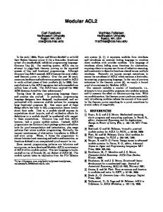
List of Figures Figure 1.1: Pictorial of the illustrative scenario of house movers: (a) Funny graphic showing the movers cooperatively moving the house; (b) Use of dollies to move an otherwise a large and heavy piece such as a car. ................................................................ 2 Figure 1.2: The visionary scenario of the autonomous modules cooperating to assist a human operator perform the moving task........................................................................... 3 Figure 1.3: Examples of cooperation in nature: (a) ants gathering food, (b) fish schooling, (c) birds flocking, (d) the great pyramids. .......................................................................... 4 Figure 1.4: Simplified CAD models of (a) An individual mobile manipulator module, and a composite system formed by (b) two modules, and (c) three modules............................ 5 Figure 1.5: Wheeled Mobile Manipulator module: (a) Detailed CAD Model; and (b) Physical prototype............................................................................................................... 6 Figure 1.6: Representative variations in topology of individual modules giving different characteristic behavior of the overall composite system .................................................... 7 Figure 1.7: Two of the many possible configurations of the payload transport system (a) a general configuration and (b) fully extended configuration ............................................... 9 Figure 1.8: Comparison of passive, active and semi-active control ................................. 11 Figure 2.1: A point P and a reference frame {O1 } located on a rigid body A in a plane with inertial frame {O } .................................................................................................... 25 Figure 2.2: Motion parameterization with the help of homogeneous transformation ...... 26 Figure 2.3: Wheeled mobile manipulator and kinematic nomeclature ............................. 32 Figure 2.4: Wheeled mobile manipulator and dynamic nomeclature ............................... 46 Figure 3.1: The Two stage implementation framework emphasizes Virtual Prototyping and Hardware-in-the-loop Physical Testing. .................................................................... 54 Figure 3.2: Virtual model of WMR with a two dof manipulator mounted on top in SolidWorks. ...................................................................................................................... 55 Figure 3.3: Equvalent model of a WMR for validation while using constant input torques ........................................................................................................................................... 56 Figure 3.4: Plot of x c and x�c versus time ........................................................................ 58 Figure 3.5: Plot of yc versus time..................................................................................... 59 Figure 3.6: Plot of x c versus yc for the circle test validation .......................................... 60 Figure 3.7: Plot of φ versus time for circle test validation .............................................. 61 Figure 3.8: Plot of θ1 and θ2 versus time for equivalent fixed base two-link serial manipulator validation case when τ1 = 10 N -mm and τ2 = 5 N-mm is applied............ 63
viii
Figure 3.9: Plot of the path followed by the end-effector when τ1 = 10 N -mm and τ2 = 5 N-mm is applied.................................................................................................... 64 Figure 3.10: Plot of θ1 and θ2 versus time for full actuation case when τR = 50 N-mm, τL = 50 N-mm, τ1 = 10 N -mm and τ2 = 5 N-mm is applied. ...................................... 64 Figure 3.11: Plot of the location of look-ahead point on the base for full actuation case when τR = 50 N-mm, τL = 50 N-mm, τ1 = 10 N -mm and τ2 = 5 N-mm is applied. 65 Figure 3.12: Plot of the location of end-effector for full actuation case when τR = 50 Nmm, τL = 50 N-mm, τ1 = 10 N -mm and τ2 = 5 N-mm is applied............................... 66 Figure 3.13: Flow-chart summarizing signal and power flow interactions (a) hardware interconnections and signal flow and (b) software instruction flow................................. 68 Figure 3.14: 3-D virtual reality based model visualization of the experiment being performed. (a) Simulink diagram for VRML model visualization; and (b) VRML model in browser.......................................................................................................................... 69 Figure 4.1: Simulink diagram to control the WMR virtual prototype .............................. 75 Figure 4.2: Straight line trajectory tracking of the base with initial error in position and velocity. (a) Desired and actual path of the WMR; (b) Error in x- and y- directions as a function of time; (c) Orientation of the base as a function of time and (d) Control torques to the right and left wheels as a function of time.............................................................. 76 Figure 4.3: Sequential snapshots of the dynamic control of virtual model while tracking a sinusoidal trajectory in vN4D (as time progress from left to right along each row). The difference between consecutive snapshots is 1 sec........................................................... 78 Figure 4.4: Sinusoidal trajectory tracking of the base with zero initial conditions. (a) Desired and actual path of the WMR; (b) Error in x- and y- directions as a function of time; (c) Orientation of the base as a function of time and (d) Control torques to the right and left wheels as a function of time. ............................................................................... 79 Figure 4.5: Sinusoidal trajectory tracking of the base with zero initial conditions and point of interest coincides with the center of mass. (a) Desired and actual path of the WMR; (b) Error in x- and y- directions as a function of time; (c) Orientation of the base as a function of time and (d) Control torques to the right and left wheels as a function of time. .................................................................................................................................. 81 Figure 4.6: Sinusoidal trajectory tracking of the base with zero initial conditions and point of interest located at a distance of 0.05 m from the center of mass. (a) Desired and actual path of the WMR; (b) Error in x- and y- directions as a function of time; (c) Orientation of the base as a function of time and (d) Control torques to the right and left wheels as a function of time.............................................................................................. 82 Figure 4.7: Sinusoidal trajectory tracking of the base with zero initial conditions and point of interest located at a distance of 0.15 m from the center of mass. (a) Desired and actual path of the WMR; (b) Error in x- and y- directions as a function of time; (c) Orientation of the base as a function of time and (d) Control torques to the right and left wheels as a function of time.............................................................................................. 83 ix
Figure 5.1: Simulink diagram to control the WMM analytical virtual prototype with a dynamic controller ............................................................................................................ 94 Figure 5.2: Straight line trajectory tracking for the base and the end-effector. (a) Desired and actual path of the Base and End-effector; (b) Orientation of the base as a function of time; (c) Base trajectory tracking error as a function of time and (d) End-effector trajectory tracking error as a function of time. ................................................................. 95 Figure 5.3: Straight line trajectory tracking for the base and sinusoidal trajectory for the end-effector. (a) Desired and actual path of the Base and End-effector; (b) Orientation of the base as a function of time; (c) Base trajectory tracking error as a function of time and (d) End-effector trajectory tracking error as a function of time........................................ 97 Figure 5.4: Straight line trajectory tracking for the base and the end-effector considering the inertia compensation in the dynamic WMM base control. (a) Desired and actual path of the Base and End-effector; (b) Orientation of the base as a function of time; (c) Base trajectory tracking error as a function of time and (d) End-effector trajectory tracking error as a function of time............................................................................................... 100 Figure 5.5: Straight line trajectory tracking for the base and sinusoidal trajectory for the end-effector considering the inertia compensation in the dynamic WMM base control. (a) Desired and actual path of the Base and End-effector; (b) Orientation of the base as a function of time; (c) Base trajectory tracking error as a function of time and (d) Endeffector trajectory tracking error as a function of time. .................................................. 101 Figure 5.6: Simulation results for end-effector and base following a straight line trajectory with kinematic trajectory tracking for the base (a) without disturbance; and (b) with disturbance;............................................................................................................. 102 Figure 5.7: Simulation results for end-effector and base following a straight line trajectory with dynamic trajectory tracking for the base (a) without disturbance; and (b) with disturbance;............................................................................................................. 103 Figure 5.8: Experimental results for end-effector and base following a straight line trajectory tracking with kinematic base controller with (a) no disturbance (b) a small T G disturbance to the end-effector at r0e = ⎡⎢ 0.9 0.3⎤⎥ m.................................................... 104 ⎣ ⎦ Figure 5.9: Experimental results for end-effector following a straight line trajectory with a dynamic trajectory tracking base controller tracing a straight line path. with (a) no T G disturbance (b) a small disturbance to the end-effector at r0e = ⎡⎢1 0.3⎤⎥ m.................. 105 ⎣ ⎦ Figure 5.10: Actual torque profile for the inputs to the right and left wheels while the base and end-effector tracks a straight line trajectory. (a) kinematic trajectory tracking control for the base (b) dynamic trajectory tracking control for the base....................... 106 Figure 5.11: Simulation results for end-effector following a sinusoidal trajectory and base following a straight line trajectory with kinematic trajectory tracking for the base (a) without disturbance; and (b) with disturbance;............................................................... 107
x
Figure 5.12: Simulation results for end-effector following a sinusoidal trajectory and base following a straight line path with dynamic trajectory tracking controller for the base (a) without disturbance; and (b) with disturbance;............................................................... 108 Figure 5.13: Sequential snapshots of the dynamic control of virtual model of WMM while the end-effector tracks a sinusoidal trajectory and base tracks a straight line trajectory in vN4D (as time progress from left to right along each row). The difference between consecutive snapshots is 1 sec. ......................................................................... 109 Figure 5.14: Experimental results for end-effector following a sinusoidal trajectory with a null-space kinematic path-following base controller tracing a straight line path. with (a) T G no disturbance (b) a small disturbance to the end-effector at r0e = ⎡⎢1 0.3⎤⎥ m (c) ⎣ ⎦ sequential photographs of the WMM captured from a recorded movie (as time progresses from left to right along each row) ................................................................................... 111 Figure 5.15: Experimental results for end-effector following a sinusoidal trajectory with a null-space dynamic path-following base controller tracing a straight line path. with (a) no T G disturbance (b) a small disturbance to the end-effector at r0e = ⎡⎢1.1 0.2⎤⎥ m (c) ⎣ ⎦ sequential photographs of the WMM captured from a recorded movie (as time progresses from left to right along each row). .................................................................................. 112 Figure 5.16: Simulation results for end-effector following a straight line trajectory and base following a sinusoidal trajectory when the base is using (a)a kinematic trajectory tracking controller; and (b) a dynamic trajectory tracking controller;............................ 114 Figure 5.17: Experimental results for end-effector following a straight line trajectory and base following a sinusoidal trajectory when the base is using (a)a kinematic trajectory tracking controller; and (b) a dynamic trajectory tracking controller;............................ 115 Figure 5.18: Torque profile for right and left motors of the WMM base as the endeffector follows a straight line trajectory and the base follows a sinusoidal trajectory when the base is using (a)a kinematic trajectory tracking controller; and (b) a dynamic trajectory tracking controller; ......................................................................................... 116 Figure 5.19: Simulation results for end-effector and base following a circular trajectory when the base is using (a)a kinematic trajectory tracking controller; and (b) a dynamic trajectory tracking controller; ......................................................................................... 117 Figure 5.20: Experimental results for end-effector and base following a circular trajectory when the base is using (a)a kinematic trajectory tracking controller; and (b) a dynamic trajectory tracking controller; ......................................................................................... 118 Figure 5.21: Torque profile for right and left motors of the WMM base as the endeffector the base tracks a circular trajectory when the base is using (a)a kinematic trajectory tracking controller; and (b) a dynamic trajectory tracking controller; ........... 119 Figure 6.1: (a) An individual mobile manipulator module, and a composite system formed by (b) 2 modules, and (c) 3 modules. ................................................................. 120 Figure 6.2: A nonholonomic mobile manipulator (NH-RR) module (a) a CAD model and (b) the corresponding schematic. .................................................................................... 121 xi
Figure 6.3: Lines of action of wrench of single mobile manipulator module for the case when none of the joints are locked. ................................................................................ 127 Figure 6.4: Lines of action of wrench of single mobile manipulator module for Case B – A-LP Module .................................................................................................................. 129 Figure 6.5: Overall system considered as: (a) independent mobile manipulators; (b) composite system. ........................................................................................................... 132 Figure 6.6: Lines of action of wrenches of two collaborative A-PP modules ................ 134
xii
List of Tables Table 3—1 Kinematic and dynamic parameters of the WMR virtual prototype.............. 57 Table 3—2 Comparison of the analytical and dynamic simulation results for WMR traveling in straight line. ................................................................................................... 59 Table 3—3 Additional kinematic and dynamic parameters of the WMM virtual prototype. ........................................................................................................................................... 62
xiii
Chapter 1
1.
Introduction
1 The overall goal of our research is to realize scalable decentralized operation in a modular and composable cooperative team of multiple wheeled robots for performing physical cooperation tasks such as transporting a common payload. We envisage variable sized groups of autonomous wheeled mobile robots (WMRs), marching in formation and cooperatively using their efforts to help manipulate and transport payloads of varied sizes and shapes. Such a modular and scalable collective of robots capable of physical interactions has many applications in extending the reach and capabilities of humans for payload transport tasks. The application arenas now span the spectrum from collective transport tasks such as hazardous waste removal to material handling to robot work crews for planetary exploration.
1.1.
Vision The interest in building smaller modules that are capable of performing physical
cooperation is motivated by the vision of using such systems to carry out tasks that are much larger, possibly more complicated and comparatively at a cheaper cost, than those that are performable with contemporary industrial single robots. Robustness and reliability of such a cooperative system is also higher when compared with a single larger robot. If one of the modules fails while performing some task, either the rest of the modules can continue to cooperate to carry out the task without any interruption or
1
another module from the inventory can be used in place of the failed module to perform the task successfully. Maintaining spare inventories of individual smaller modules to replace the failed vehicles in such situations are also cheaper compared to when using larger robots for bigger tasks. Also, tasks that cannot be performed by individual robots could be made feasible and more economical by leveraging advantages of mass production of smaller robots. Moreover, when multiple mobile robots cooperate to transport a payload, they form a parallel structure which is in general robust compared to serial structure. Various facets of this vision are explained and illustrated further by the following two scenarios.
1.1.1.
Furniture movers scenario
www.kingdolly.com http://www.harriscanvascamp.com/
(a)
(b)
Figure 1.1: Pictorial of the illustrative scenario of house movers: (a) Funny graphic showing the movers cooperatively moving the house; (b) Use of dollies to move an otherwise a large and heavy piece such as a car.
Consider an illustrative scenario of household furniture movers while they move large piece of furniture (payload). Traditionally, such movers employ a variable number of modular wheeled dollies, as determined by the size and weight of the payload that they 2
are moving. These dollies are positioned at suitable locations to ensure mobility, stability and appropriate load distribution. Sometimes dollies are added to or removed from the existing set of dollies used depending on the path to be taken to move the furniture. Oftentimes, the locations of these dollies are re-adjusted to avoid obstacles and to enhance overall moving performance. Figure 1.1(a) is an illustrative pictorial representation furniture/house movers suggesting the need and benefits of cooperation. Figure 1.1(b) illustrates a more realistic picture of how wheeled dollies can be used to move a large and heavy payload from one location to another with minimal effort. This process of payload manipulation and transport can be greatly enhanced by adding some level of intelligence to the dollies. These intelligent and (fully- or semi-) autonomous dollies can then cooperate to either assist the human operator or autonomously perform the moving operation. Figure 1.2 illustrates the visionary scenario of the autonomous modules cooperating physically to assist a human operator perform the task of moving a large and heavy payload from one location to another.
Figure 1.2: The visionary scenario of the autonomous modules cooperating to assist a human operator perform the moving task.
3
1.1.2.
Biological precedents Alternately, one may also consider the examples of cooperation from nature.
Biologists who study animal aggregations such as swarms, school, flocks, and herds have observed the remarkable group-level cooperative achievement of tasks. For example, armies of ants (Figure 1.3(a)) leverage the collective strength and manipulation capabilities to be move large food-pieces, which would be impossible for a single ant. In a similar way, school of fish (Figure 1.3(b)) cooperatively performs complicated maneuvers to avoid such predators as sharks. One more example is when birds like geese or ducks fly in a “V” shaped formation (Figure 1.3(c)) to avoid tiring quickly and thus flying longer distances. Figure 1.3(d) shows the great pyramids of Egypt that is a remarkable testimony to human cooperation since ancient times.
(a)
(b)
(c)
(d)
Figure 1.3: Examples of cooperation in nature: (a) ants gathering food, (b) fish schooling, (c) birds flocking, (d) the great pyramids.
In all the above examples, the emphasis is on accomplishment of a large and complex task requires cooperation among different members of a team. Thus, our vision 4
is to create a framework for cooperative payload manipulation with a team composed of many autonomous wheeled mobile modules, controlled as a collective while possessing the ability to reconfigure to enhance performance.
The emphasis on physical
collaboration in such physically-coupled collectives imposes more stringent constraints than encountered in many other collective robotics efforts that focus on information collaboration for foraging, map building and reconnaissance. However, the increased flexibility, cost effectiveness, robustness and reliability achieved by replacing a single larger material handling device by a fleet of smaller modules achieving equal or better overall performance is very attractive. The proposed application arenas range from household furniture moving to industrial material handling applications, where variable numbers of such modules can be employed to manipulate different shape and weight payloads, to extra-terrestrial applications, where individual rover modules sent on separate missions can cooperate to support planetary colonization efforts. Figure 1.4 shows simplified CAD drawing of different number of modules being employed to perform a desired payload transport job depending on the weight and size of payload.
(a)
(b)
(c)
Figure 1.4: Simplified CAD models of (a) An individual mobile manipulator module, and a composite system formed by (b) two modules, and (c) three modules.
5
Our basic module is a Wheeled Mobile Manipulator (WMM) that consists of a WMR with a two degrees-of-freedom (dofs) manipulator arm mounted on the mobile base at a suitable location. Figure 1.5(a) depicts a detailed CAD model of the WMM[1] and Figure 1.5(b) shows the actual physical prototype that has been constructed in ARMLab and will be used to perform the experimental studies presented in this dissertation. The WMR is a differentially driven disk-wheeled platform and uses a set of passive MECANUM wheels to support the weight without resisting the dofs. . The mounted manipulator arm has two active revolute joints with axes of rotation parallel to each other and perpendicular to the mobile platform (and the ground). The end-effector is a flat plate supported by a passive revolute joint that ensures that no moments can be transferred to the manipulator-arm.
(a)
(b)
Figure 1.5: Wheeled Mobile Manipulator module: (a) Detailed CAD Model; and (b) Physical prototype
1.2.
Research Challenges In spite of all these advantages, the direct applicability of such cooperative
systems is very limited mainly due to the many research challenges that still need to be addressed. We categorize the different challenges posed for such a physically cooperating
6
system in two broad categories: (i) design related challenges; and (ii) control related challenges.
1.2.1.
Design In the design and implementation of our cooperative transport system, we
consider a compositional approach to creation of a modular system. Modularity can come from either use of modular physical components or from the use of modular software components and the ability to easily switch from one module to another module. Physical modularity may now be achieved in terms of topology, dimensions and configuration as will be briefly discussed below. Topology:
(a)
(b)
(c)
Figure 1.6: Representative variations in topology of individual modules giving different characteristic behavior of the overall composite system
Many different types of individual module designs are possible. Figure 1.6 shows a small representative set of various possible configurations of individual modules which gives different characteristic behavior of the overall composite system. WMR mounted with a single dof manipulator as shown in Figure 1.6(a) is able to accommodate
7
disturbances only in directions instantaneously tangential to the location of the joint when used in a composite system. Topology of the composite system must be considered very carefully during the design stage, since it affects the overall performance of the cooperative system and is difficult, if not impossible, to make significant changes at a later stage. Dimensions: The choice of selecting the dimensions significantly affects the workspace and payload carrying capacity of the WMM. This includes selection of kinematic parameters like link lengths, base dimensions, radius of wheels, distance between two wheels, location of mounting the manipulator etc. However, by suitably designing the adjustable length links and mountings, some of these choices can be used to offer more flexibility at the operational stage. Configuration: A cooperative system transporting the payload is a highly redundant system. For a given location and orientation of the payload, there are infinitely many possible locations of individual modules that are cooperating to transport the payload. The relative locations of each modules in the configuration has significant impact on various performance measures like the load carrying capacity, manipulability, ability to accommodate and reject disturbances, etc. For instance, the fully extended configuration shown in Figure 1.7(b) may not be able to accommodate the disturbance in all directions where as the configuration of Figure 1.7(a) will be able to accommodate the disturbances in any given direction relatively easily.
8
(a)
(b)
Figure 1.7: Two of the many possible configurations of the payload transport system (a) a general configuration and (b) fully extended configuration
1.2.2.
Control The control and reconfiguration of the cooperating robots pose challenges due to
the nonholonomic constraints arising because of use of wheels, redundancy in actuation as well as configuration, formation of parallel structure due to the creation of closed kinematic-chains, coupling between the dynamics of the base and the manipulator in single WMM, dynamic coupling between different cooperating WMMs, and other challenges. Centralized and decentralized Centralized control employs a single control routine that is responsible for monitoring and controlling every robot in the collective. Thus, the controller must have exact model of the composite system as well as complete state information of the entire collective to implement control. Hence, addition or removal of modules while using a 9
centralized controller is difficult since it requires a new model of composite system to be downloaded. A centralized controller is less scalable since the communication requirement increases drastically as more and more modules are added (as it requires the full state information from all modules before determining control). Another disadvantage is that the system is not redundant from a control standpoint. If the central control routine fails then the collective fails. In contrast, a decentralized control distributes the control routines, partially or completely, to the individual modules of the collective. This method is less efficient because less information is known about each robot, so exact control and path planning of all robots is more difficult. Sometimes it has a degrading effect in the sense that the modules may work against each other creating unnecessary internal forces. However, the advantages are increased modularity and redundancy. Robots can now easily be added or subtracted from the collective without modifying any system model or control routine. This method is also more robust because if one control routine fails, then only one robot is affected, while the rest of the collective still remains functional. Redundancy resolution In this work, we consider the task for the cooperative system to be to transport a payload from one location to another in a planar workspace. If we consider only the location of a certain point on the payload to be transported, such as task is a two dofs task. If the orientation of the payload is also included, then the dimension of the task space is three. The proposed manipulator has in general five dofs and instantaneously four degrees of freedom (since the nonholonomic constraint reduces one instantaneous dof). Hence, the manipulator is by definition, kinematically redundant. Such redundancy
10
is important since it increases dexterity and versatility of the modules and can be used to avoid obstacles and kinematic singularities or to optimize some performance objective. However, the use of a systematic method of resolving such redundancy becomes extremely important. Active, passive and semi-active Figure 1.8 shows different types of control based on type of actuation used to control the interaction between different modules. Passive control employs use of passive structural members like link-lengths or spring constants to produce desired dynamic behavior at the interface. The benefits include increase in the control bandwidth and often reduction in energy required. However, selection of various physical parameters like linklengths and spring constants must be done carefully. Additionally, the effective range of operating conditions tends to be limited and the passive structural members must be replaced if the desired behavior of the system changes significantly.
(a)
(b)
(c)
Figure 1.8: Comparison of passive, active and semi-active control
In contrast, active control uses the sensors to detect various states/output of the system, based on which one can modify the input to get desired output. Different types of active control techniques like, PID control, Augmented PD control, Computed-torque control, etc. exist. Most of these techniques rely on good, if not perfect, knowledge of the kinematic/dynamic parameters of the system to be controlled. Active force control has also proven to be difficult, especially while working with stiff environments. A 11
commonly observed limitation is guaranteeing stability of the system while using active control. Semi-active control, which modifies the system properties, has many advantages of active and passive systems. Like passive systems, such semi-active systems are passive at the end-effector, possess high bandwidth and require relatively less power to control. Like active control, semi-active control can now be used for wider range of operations, can control the performance of the system in an active way and can be re-programmed to suit new applications and modify desired behaviors/performance relatively easily. However, compared to electro-mechanical counterparts, components used for semi-active control tend to have a slower adaptation/control rate. Semi-active components also add secondary dynamics (and additional dof) to the main system and thus make it more difficult to control than direct active control. When we consider the overall cooperative payload transport system, by changing the relative configuration, we are in fact changing the physical properties of the collective like inertia, mass distribution as well as non-physical properties like manipulability, force rejection ability and directions etc. Hence, our control, despite being an active control that uses motors at every joint, can be categorized as semi-active control.
1.3.
Literature search A lot of research work has been done in the past three decades in the filed of
mobile robots, especially the WMRs. Some of these works also deal with the WMMs of the type that we consider in this dissertation. Relatively less work is done on cooperating WMM to perform a desired payload transport task. In this section, we present a review of
12
such works and some of the drawbacks of existing approaches to control of individual and groups of WMMs.
1.3.1.
Individual WMM A mobile manipulator consists of a mobile robot with one (or more) mounted
multi-dof manipulator arms. Many variants of such systems are possible, based on the nature of the mobile base (gantry system, another manipulator[2] or some wheeled or tracked platform) and the nature of the mounted manipulator (number and actuation of the articulations). Resulting significant increases in mobility and available workspace have promoted numerous applications, especially for WMMs [3-9]. While robust physical construction, ease of addition to platforms and ease of operation make disk wheels popular, the kinematics of rolling contact of the various wheels with the terrain creates nonholonomic constraints and the resulting class of nonholonomic WMMs requires special treatment. Our mobile base consists of a wheeled mobile platform. A composite multi-dof wheeled vehicle is formed when a payload is placed at the end-effectors of multiple such modules. However, two or more WMRs, with rigid axles, cannot be arbitrarily coupled to each other due to the incompatibility of the velocities of the wheels. The potential degradation in the overall performance can range from loss of mobility, rattle-shake, unintentional compliance, wear and tear of the tires and wheel slip. Hence, many approaches in the literature [10, 11] advocate the addition of further articulations between the various wheels/axles in order to accommodate the rigid body constraints – the role played by the mounted planar manipulator arm. In general, a careful selection of the type, number, dimensions and actuation of both the wheels attached to the base and the joints in the mounted manipulator are critical to determining the individual 13
module performance as well as the performance of the composite system [12, 13]. The resulting composite vehicle, of the form shown in Figure 1.4, possesses: (i) ability to accommodate changes in the relative configuration (by virtue of the compliant linkage); (ii) a mechanism for detecting such changes (using sensed articulations); and (iii) means to compensate for such disturbances (using the redundant actuation of the bases), while performing the payload transport task. The nonholonomic constraints that arise due to the wheeled platform are representable as first order non-integrable differential equations in Pfaffian form, permitting the state equation to be written in the form of a drift-free affine system. Considerable literature in the field of control of nonholonomic WMRs has focused on developing feedback control laws to tackle three principal problems: posture tracking; path following; and the more difficult posture stabilization. The inability of WMRs to be stabilized to a single equilibrium point by a continuous (smooth) time-invariant pure state feedback law (due to the violation of Brockett’s condition [14]), has led to numerous approaches involving either discontinuous time-invariant feedback laws or continuousvarying non-linear feedback control laws. Other strategies motion planning and control of drift-free affine systems by conversion to canonical representations, such as chained systems [15], have also been explored. See [16-18] for further details. While, many of the above approaches were developed for the kinematic steering problem of WMRs, operating under the assumption that perfect velocity tracking would be possible, other approaches [19, 20] explicitly take into account the dynamics of the actuators and the mobile robot in generation of the control laws. Integrator backstepping approaches [21],
14
to implement computed-torque controllers that ensure convergence to the desired velocities prescribed by the kinematic control schemes, have also been pursued. Combining the mobility of the base platform and the mounted manipulator creates both kinematic and actuator redundancy. The determination of the actuator rates/forces for a given end-effector motions/forces in a redundant manipulator is typically an underconstrained problem but essential for motion planning/control of such systems. See Nakamura [22] for a review of these methods. At the kinematic level, redundancy results since the combined system may possess more degrees of freedom than necessary. Many schemes have been proposed with an underlying theme of optimizing some measure of performance based on kinematics (and in some cases extended to include the dynamics). These results, developed for serial-chain manipulators, have been extended and applied in the context of mobile manipulators. For example, the augmented Jacobian approaches exemplified by Seraji [6] extended Whitney’s [23] approach to kinematic redundancy resolution of mobile manipulators. Alternatively, the decoupled Jacobian approaches, exemplified by Yamamoto and Yun [8] decompose the motions of the mobile manipulator into decoupled WMR-base and manipulator subsystems. The WMR is then controlled so as to bring the manipulator to a preferred configuration (using criteria such as the manipulability measure) as the end-effector performs a variety of unknown manipulation tasks. However, as Wang and Kumar [24] note, if the augmented Jacobian is not the Jacobian of a kinematic function f (q ) , the resulting trajectories may not be globally integrable. The decoupling approach lends itself better to decentralized planning and control of the mobile base and the manipulator arm. However, in either case, the
15
kinematic-level redundancy resolution implicitly assumes the availability of good ratecontrol actuators. However, far lesser literature discusses dynamic-redundancy resolution within the articulated chain. In exactly-actuated systems, only as many components of the motions/forces as degrees of actuation can be controlled. However, in redundant systems, it is meaningful to exploit the surplus actuator inputs to achieve secondary goals, in addition to primary task performance. Traditionally such secondary criteria have included either the contact- or internal-force distribution – this giving rise to the various hybrid position/force control schemes frequently seen in multi-arm systems [25-27]. Some extensions of the decoupled Jacobian approach to kinematic redundancy resolution have also been pursued for dynamic redundancy resolution. Fully actuated mobile manipulators have been examined to study of the effect of the dynamic interaction between the manipulators and the mobile platform on the task performance [8]. It is noteworthy that the location of the manipulator arm relative to the mobile base has considerable effect on the performance of a mobile manipulator and needs to be carefully considered [3, 5]. However, the approach adopted in our work is to consider the alternate partitioning of the dynamics into a task/end-effector motion space and an internal/nullmotion space, under an appropriately defined metric. Such a partitioning, defined in terms of a metric endowed by the kinetic energy of a simple mechanical system, can formally be shown to be orthogonal and decoupled [28]. Khatib [29] proposed a method of controlling redundant serial-chain systems by projecting the system dynamics into the task-space to realize an end-effector dynamic model together with a dynamically16
consistent actuation that provides decoupled control of joint motions in the null space. This was subsequently extended for mobile manipulator systems with holonomic bases and fully actuated manipulators [9]. Similarly Tan et al. [30] controlled a similar holonomic mobile manipulator to manipulate a passive nonholonomic cart along straight lines, corners or sinusoidal trajectories. However, the presence of the non-holonomic base creates challenges for control of end-effector motion/force outputs in task-space. Realizing this capability is a critical precursor to our longer-term goal of decentralized payload manipulation operations by the nonholonomic WMMs and will be the focus of our work.
1.3.2.
Cooperative system Cooperative multi-robot systems, ranging from multiple mobile robots [31, 32],
multiple manipulators [33], multi-fingered hands [26, 34] and multi-legged vehicles [35, 36] have been extensively studied in a variety of contexts. We restrict our attention to cooperative physical manipulation by articulated WMMs focusing on the motion and force distribution issues. There is relatively less literature, but considerably greater variability, in the approaches employed for cooperation of multiple mobile manipulators [9, 37-40]. Khatib et al. [9] developed a decentralized control structure for cooperative tasks with mobile manipulation systems with holonomic bases and fully actuated manipulators. Motion planning has also been considered for collaborating teams of nonholonomic mobile manipulators from various centralized perspectives [37, 38]. Kosuge et al. [39] propose a simple method for carrying a large object by cooperation of multiple mobile manipulators with impedance based controllers by selectively locking and unlocking some joints of the 17
mounted manipulators on mobile platforms. Yamakita et al. [40] implement the Passive Velocity Field Control approach for the cooperative control of multiple mobile robots holding an object. In almost all these cases, the principal emphasis is on control of a system formed with generic WMM modules. Despite the significant influence on the overall system performance, typically scant attention is paid either the nature of the module (type, dimensions or actuation of the wheels and/or the articulations), a shortcoming that we begin to address in this paper. On a slightly different note, we also see that the composite system formed by connecting the multiple mobile manipulators to the common payload share many features with the class of Multi-Degree-of-Freedom (MDOF) Wheeled Vehicles [10, 41-46]. While some of these like the RollerRacer [41] and the Snakeboard [42] are case-studies in underactuated locomotion, several others like OMNIMATE/CLAPPER [10] and systems with multiple actively steered wheels [43-45] and WAAVs [46] feature redundancy in actuation. Several of these authors also note that despite gains in maneuverability over conventional mobile robots, the overconstrained nature with hybrid series-parallel kinematic chains creates challenges in design, planning and control of such systems. The twist- and wrench-based analysis methods adopted in this paper offer convenient tools for systematic system-level motion- and force-analysis based on the capabilities of the individual modules.
1.4.
Contribution A systematic (and quantitative) framework for evaluation of the individual
module- and system-level characteristics is desirable and remains one of the underlying goals of our research efforts. 18
1.4.1.
Design In general, it is desirable to have a systematic procedure to design a system.
However, in most situations, there are multiple needs with variable importance and many more design options and it is not always feasible to have a single solution that satisfies all the prioritized needs. In such cases, it becomes important to be able to evaluate the performance of the system with certain design choices in simulation, possibly eliminate some of these choices and pick a suitable starting design choice to construct the physical prototype for further refinement. We use a virtual analysis framework and develop a virtual prototype that allows performing these initial refinements of the WMM. How can we systematically analyze, analytically compare and either eliminate or refine the many available design choices for the hardware platform (individual as well as cooperative) for the payload transport case? Development of virtual framework In this dissertation, we develop a virtual framework that allows parametric studies on the performance evaluation and capability of an individual WMM and the composite cooperative system in physics based co-simulation environment. We use this framework to initially determine the location of the Joint1 of the mounted manipulator on the WMM base. We also use this framework to evaluate the performance of the initial dynamic controller for the base of the WMM. After observing the poor performance of the controller, we further refine it to include the inertia and reaction force effects of the mounted manipulator.
19
How do the actuation schemes of the individual modules affect the performance of the payload manipulation cooperative system composed of either homogeneous or heterogeneous modules? Systematic modeling of cooperative WMM system for static analysis The choice of the type and number of actuation influences not only the performance of a single WMM, but also of the composite system. We develop a systematic framework for formulation and evaluation of system-level performance of a cooperative payload transport task by a modularly composed system of multiple WMMs using screw-theoretic analysis tools. Specifically, we present a method for the systematic modeling of the novel nonholonomic WMM modules (which form the serial-chain arms/legs); the systematic system-level motion- and force-capability analysis based on capabilities of the individual modules and subsequent analysis of the effects of selection of the actuation at the articulations (active, passive or locked) on system performance. In particular, by analyzing a 2-module composite system, we illustrate how a marginal change in the selection of actuation within the system can significantly affect the overall performance. The analysis also led to the selection of a candidate system-configuration capable of accommodating and correcting motion and force-disturbances applied at the payload. The overall framework employed here may also be easily extended to treat larger composite system implementations with more mobile manipulator modules. We use this methodical analysis tool to answer the following design questions. •
Can the system accommodate arbitrary payload motions?
•
Can the system create arbitrary payload motions?
•
Can the system resist arbitrary payload forces?
•
What effect do various actuation schemas have on payload manipulation performance? 20
1.4.2.
Control A WMR cannot be arbitrarily coupled with other WMRs to perform a physical
cooperation tasks since it is prone to jerky motion and wheel slippage. In order to avoid these problems and allow for some accommodation, we introduce additional articulations in the design of our WMR in the form of a multi-link manipulator. Such interface with active/passive/locked joints and sensed articulation also helps detect disturbances that come because of any particular WMM. However, when the system is carrying a payload, each WMM module along with the payload mounted on top of the two d-o-f manipulator forms a closed loop, thus adding holonomic constraints and redundancy to the composite system. How can we take advantage of the redundancy and the presence of nonholonomic constraints and develop a dynamic control algorithm (that decouples the task space and redundant null space inputs) to control the WMM? How does this algorithm behave when compared with a kinematic control algorithm in simulation as well as in experimentation? The coupling of the nonholonomic base constraints and the inherent redundancy in nonholonomic WMMs create significant challenges for control of end-effector (motion/force) interactions. We present a solution approach leverages the kinetic-energy metric of the underlying articulated mechanical systems to create a dynamicallyconsistent and decoupled partitioning into external (task) space and internal (null) space dynamics. The primary task is assumed to be one of controlling the motion and/or force interactions of the end-effector with respect to the attached payload/external environment. The secondary task is assumed to be one of controlling the surplus degreesof-freedom within the system (relative pose of the mobile base).
21
Such a systematic approach to resolution of the redundancy while allowing for internal reconfiguration is key to many of the current and envisaged applications for such systems. These algorithms are then evaluated within an implementation framework that emphasizes both virtual prototyping (VP) and hardware-in-the-loop (HIL) testing. Simulation and experimental results are used to highlight aspects of implementation in a real-time sensor-based control framework to help fully exploit the novel capabilities of such nonholonomic WMMs. Finally, a comparative study of the two different types of controllers for the base, a kinematic trajectory tracking controller and a dynamic trajectory tracking controller in terms of trajectory tracking performance and torque requirements is also done for various kinds of trajectories ranging from a straight line trajectory to sinusoidal trajectory to a circular trajectory and different combinations of these trajectories prescribed for the endeffector and the look-ahead point on the base.
1.5.
Dissertation organization In this chapter, we presented our guiding vision that directs the research in this
project of cooperative payload transport. We then presented a brief discussion of the various challenges faced and a review of contemporary research in the filed of WMRs, WMMs, cooperative payload transport and other related field such as multi-fingered hands and multi-legged robots. We then discussed the contribution of this dissertation. The remaining of this dissertation is organized as follows. Chapter 2 introduces the notation and discusses the mathematical tools used in the dissertation. Kinematics and Dynamics of WMMs (and WMRs) are then developed in
22
this section. A discussion of projecting the equations of motion on the feasible motion space and constraint force space is also presented. Chapter
3
presents
the
virtual
prototyping
and
hardware-in-the-loop
implementation framework. Validation of the virtual prototype model of WMM and WMR (created in visualNastran 4D) is also performed. A VRML based web-interface for visualization of the experimental results as it is being formed is also developed in this chapter. Chapter 4
presents the dynamic control algorithm for the control of the
nonholonomic WMR. This control algorithm is validated using the virtual prototype and results are presented. Chapter 5 discusses the dynamic control algorithm for the Wheeled Mobile Manipulator that decouples the task-space dynamics and the null-space dynamics. A kinematic trajectory tracking algorithm and a dynamic trajectory tracking algorithm are then discussed for controlling the dynamics of the base of WMM. These algorithms are then implemented on virtual and physical prototype of the WMM and the results are presented. Chapter 6 presents the cooperative system analysis and discusses the effects of active,
locked
and
passive
joints
on
the
force
and
motion
disturbance
rejection/accommodation capability of the combined system. Finally we conclude the dissertation in Chapter 7 and discuss some avenues of future work.
23
Chapter 2
2. Kinematics, Statics and Dynamics of a Wheeled Mobile Manipulator
2 Researchers in the field of articulated multibody systems have looked at various approaches towards their study, analysis, and control. Screw-theoretic approach, configuration-space approach, and graph-theoretic approach are just a few examples of these different ways to analyze and study the articulated multibody systems. In this chapter, we briefly describe the basis of the screw-theoretic framework and then introduce the tools used to perform kinematic and static analysis within this framework. The same approach can be used to study and analyze the dynamics of multibody systems. [47, 48] However, due to the ease of formulation and reduced complexity, we use the joint configuration-space to develop the articulated dynamics framework.
2.1.
Rigid-body motions A rigid-body consists of particles that maintain a fixed relative distance to each
other at all the times. A general rigid-body motion consists of translations and rotations that satisfy the rigidity requirements. The position of point P as expressed in {O } can be given as G G G rP = R1 1rP + r01
24
(2.1)
G where r01 is the represents the position vector of the location of the origin of frame {O1 } G G in an inertial frame, 1rP is the position vector of point P in the frame {O1 } , while rP is the position vector of the same point P in inertial frame {O } .
xˆ1
yˆ1
{O1 }
G r01
A
P
G G rP = rP
yˆ0
{O }
G rP
1
0
xˆ0
Figure 2.1: A point P and a reference frame {O1 } located on a rigid body A in a plane with inertial frame {O }
The homogeneous matrix representation of equation (2.1) can be given as
G ⎡R1 r01 ⎤ ⎢ ⎥ 0 A1 = A1 = ⎢ GT (2.2) ⎥ 1⎥ ⎢0 ⎣ ⎦ where A ∈ SE (2) that takes a point or vector in coordinate frame {O1 } and expresses it G in coordinate frame {O } , 0 is an appropriate dimensional (here, 2 dimensional) columnvector of zeroes, R1 is a rotation matrix with the following properties: •
R ∈ SO (2) and R−1 ∈ SO (2)
•
R−1 = RT 25
•
det {R} = +1
Inverse of the homogeneous matrix A is given as −1
A0 = [A1 ]
1
⎡R1T ⎢ = ⎢ GT ⎢0 ⎣
G −R1T r01 ⎤ ⎥ ⎥ 1 ⎥ ⎦
(2.3)
Figure 2.2: Motion parameterization with the help of homogeneous transformation
In order to perform useful and meaningful operations with algebraic quantities like position, velocity, acceleration, etc., each of the quantities must be expressed in the same coordinate reference frame. Above transformations can be used to transform the quantity from one frame to another.
2.2.
Screw Chasles proved that a rigid body can be moved from any one position to any other
position by a movement consisting of rotation about a straight line followed by 26
translation parallel to that line. Such a motion is called a screw motion and serves as a convenient compact notation to describe rigid body motions. The main advantage in using screws, twists, and wrenches to describe rigid body kinematics is that they allow a global description of rigid body motion which does not suffer from singularities due to the use of local coordinates. We briefly summarize the planar twist-based modeling of the articulated mechanical systems here. An interested reader may refer to Hunt [49] for the more traditional line-based screw-theoretic modeling
2.2.1.
Velocity twists The infinitesimal version of a screw motion is called a twist and it provides a
description of the instantaneous velocity of a rigid body in terms of its linear and angular components. The velocity twist of a rigid body expressed at point P can be represented as
⎡ω⎤ G tP = ⎢⎢ G ⎥⎥ (2.4) v P ⎣⎢ ⎦⎥ G where vP is the linear velocity of the rigid body expressed at point P and ω is the angular velocity of the body. For a general 3D case ω is a 3 dimensional vector however, for the case of planar motion, we will be always concerned with ω as a scalar, that defines the rotation about the z axis. We consider a general planar case where A1 (t ) ∈ SE (2) is a one-parameter curve (parameterized by time) representing a trajectory of a rigid body, more specifically, the rigid body motion of the frame {O1 } attached to the body, relative to the fixed inertial frame.
We can now determine the spatial (inertial) twist matrix T ∈ se (2) by
performing following operations: 27
⎡R� RT −R� RT rG + rG� ⎤ 1 1 01 01 ⎥ ⎢ 1 1 −1 � T1 = T1 = A1 [A1 ] = ⎢ G (2.5) ⎥ ⎢ 0T ⎥ 0 ⎣⎢ ⎦⎥ All the quantities in above equation are expressed in a spatial (or inertial) frame of 0
0
� � reference. Here, R� 1R1T is a screw-symmetric matrix also denoted by 0 ω10 = ω1 and is
given as
⎡ 0 −ω1 ⎤ � ⎥ (2.6) ω1 = ⎢⎢ ⎥ 0 ω 1 ⎣⎢ ⎦⎥ where 0 ω10 = ω1 is the angular velocity of the rigid body with respect to inertial frame as
G G expressed in the inertial frame. We can also rewrite the expression −R� 1R1T r01 + r�01 as G G G G G � v 01 = −R� 1R1T r01 + r�01 = v01 + ω1 (−r01 )
(2.7) G −r01 is a vector that instantaneously refers to the origin of the inertial frame and G so v 01 is the velocity of the point on the body with frame {O1 } that is instantaneously
located at the origin of the inertial frame and expressed in the inertial frame of reference. The spatial twist matrix can thus be represented as
⎡ ω�10 vG0 ⎤ 1 ⎥ ⎢ T1 = ⎢ GT (2.8) ⎥ ⎢0 0⎥ ⎣ ⎦ An alternative method of expressing the twist matrix in body fixed frame is given by ⎡RT R� RT rG� ⎤ ⎡ ω� 1 vG 1 ⎤ 01 1 01 ⎥ ⎢ 1 1 −1 ⎢ 1 ⎥ (2.9) T11 = [A1 ] A�1 = ⎢ G = ⎢ GT ⎥ ⎥ T ⎢ 0 ⎥ ⎢0 0⎥ 0 ⎦ ⎣⎢ ⎦⎥ ⎣ �1 where ω1 a screw-symmetric matrix similar to the expression (2.6) whose components 0
ω11 = ω11 represents the angular velocity of the rigid body as expressed in the body fixed
G G G frame, in this case, frame {O1 } . v 011 = R1T v 01 = 1R0v 01 represents the velocity of the
28
origin of the body frame {O1 } as expressed in the body frame {O1 } . A twist vector can be extracted from the twist matrix which serves as the compact notation for representing instantaneous velocity of a moving body. A twist vector can be extracted from either
G G inertial twist matrix or body fixed twist matrix. The twist vector 0t1 = t1 extracted from the inertial twist matrix is given as
G G TT t1 = ⎡⎢ ω1 ⎡⎢v 01 ⎤⎥ ⎤⎥ (2.10) ⎣ ⎦ ⎦ ⎣ G and the twist vector t11 extracted from the body fixed twist matrix can be given as G G TT t11 = ⎡⎢ω11 ⎡⎣⎢v 011 ⎤⎦⎥ ⎤⎥ (2.11) ⎣ ⎦ G G Some authors prefer the notation of a twist vector where t = (v , ω ) , however, our G G preference is t = (ω, v ) . The twist matrix, as discussed above, can be developed in either the body fixed frame or the inertial frame of reference. When it is desired to transform the twist matrix to any other frame of reference, a similarity transformation is used. Thus, the twist matrix
T10 referenced in inertial frame can now be expressed in any general frame {Ob } by
0
T1b = Ab−1 0T10Ab
0
(2.12)
where the matrix Ab represents the homogeneous transformation matrix from the inertial frame to {Ob } . Next, we are interested in determining the relationship of the two different types of representation of twist vector, namely inertial twist vector and spatial twist vector. ω1 = ω11 G G G G � � G v 01 = v 01 + ω1 (−r01 ) = R1v 011 − ω11 (r01 )
29
(2.13)
G G Spatial twist t1 and body fixed twist t11 can thus be related with the help of twist G G adjoint transform as t1 = Γ1 ⎡⎢t11 ⎤⎥ where the adjoint transform 0 Γ1 = Γ1 is given as ⎣ ⎦
⎡ 1 0T ⎤ ⎢ ⎥ ⎥ (2.14) Γ1 = ⎢ G T G ⎤ R⎥ ⎢ ⎡r r − 1⎥ x 01 ⎥ ⎦ ⎣⎢ ⎣⎢ y 01 ⎦ The adjoint matrix Γ1 maps body velocity twist coordinates to spatial velocity twist coordinates. Γ1 is invertible and its inverse is −1
[Γ1 ]
2.2.2.
G ⎤⎤ ⎡ ⎡G ⎢1 ⎢⎣ry 01 −rx 01 ⎥⎦ ⎥ T = ⎢G = Γ ⎥ [ ] 1 T ⎢0 ⎥ [R1 ] ⎣⎢ ⎦⎥
(2.15)
Force wrenches and reciprocity Poinsot discovered that any system of forces acting on a rigid body can be
replaced by a single force applied along a line, combined with a moment about that same line. Such a force is referred to as a wrench. Wrenches are dual to twists, so that many of the results that apply to twists can be extended to wrenches. A generalized wrench w acting on a body can be represented by a force-moment pair as GT G ⎡⎢ f ⎤⎥ (2.16) w=⎢ ⎥ ⎢⎣ m ⎥⎦ Just like the twists, the values of the wrench vector depend on the coordinate
frame in which the force and moment are represented. However, we consider all the calculations relative to a single coordinate frame and omit the use of subscripts. Wrenches combine naturally with twists to define rate of work done. The power (or rate G G of work done) by a wrench w = ⎡⎢ f T ⎣
G G m ⎤⎥ on a twist t = ⎡⎢ω v T ⎤⎥ is given by ⎦ ⎣ ⎦
30
m GT G ⎡ G ⎤ ⎡⎢ ⎤⎥ P = t ∆w w = ⎢w v ⎥ ⎢ G ⎥ ⎣ ⎦⎢f ⎥ ⎣ ⎦ Alternatively, one can also write
where ∆w and ∆t are given as
G ⎡v ⎤ GT G ⎡ G ⎤ ⎢ P = w ∆tt = ⎢ f m ⎥ ⎢ ⎥⎥ ⎣ ⎦ ⎢w ⎥ ⎣ ⎦
⎡0 ⎢ ⎢ ∆w = ⎢1 ⎢ ⎢0 ⎢⎣ The reciprocity relationship
(2.17)
(2.18)
⎡ 0 1 0⎤ 0 1⎤⎥ ⎢ ⎥ ⎥ ⎢ ⎥ (2.19) 0 0⎥ and ∆t = ⎢ 0 0 1⎥ ⎥ ⎢ ⎥ ⎢ 1 0 0⎥ 1 0⎥⎥ ⎢⎣ ⎥⎦ ⎦ D between a wrench and a twist can be defined when
instantaneous work done P is identically equal to zero. Thus,
G G w D t = fx vx + fy vy + mz wz = 0 The above statement is the well-known Principle of Virtual Work.
2.3.
(2.20)
Kinematics of WMM A manipulator can be schematically represented from a mechanical viewpoint as a
kinematic chain of rigid bodies connected by means of (generally revolute or prismatic) joints. The kinematics of a robot manipulator describes the relationship between the motion of the joints of the manipulator and the resulting motion of the rigid bodies which from the robot. Moreover, wheeled systems, because of the rolling contact between the wheel and ground, are subject to nonholonomic constraints. These constraints can be represented at velocity level and thus becomes an essential element of kinematic analysis of a WMM of the type shown in Figure 2.3. Next, we develop the kinematic model and the terminology for the WMR and the WMM that will be used in subsequent dynamic analysis. First, we consider the WMR
31
alone and its non-holonomic constraints.
Then we consider the addition of the
manipulator and develop all necessary kinematic relationships. Finally, we assemble the constraint matrix, the nullspace matrix, and construct a Jacobian matrix which relates the task-space to the joint space.
Figure 2.3: Wheeled mobile manipulator and kinematic nomeclature
Consider a WMM in described in an inertial frame {O } as shown in Figure 2.3. Frame {Ob } , at an angle φ with respect to the {O } , is located at the center of mass of the base with its xˆb axis oriented in the direction of the forward motion of the base. The
G position vector of the center of mass can thus be expressed in inertial frame as r0b . The 32
mobile base is actuated by two independently driven collinear wheels with radius r located on an axis at a distance d ≥ 0 from the center of mass. The two wheels are separated by a distance of 2b . Let L1 and L2 be the lengths of two links, Link1 and Link2, with center of mass located at a distance Lcm 1 and Lcm 2 respectively. The frames
{Ocm 1 } and {Ocm 2 } are located at the respective center of mass. The proximal end of Link1 is mounted on the wheeled mobile base at a distance La from the center of mass along the +xˆb axis and distal end is connected to Link2. θ1 is the relative angle between the frame {Ob } and Link1 and θ2 describes the relative orientation of the Link2 with respect to Link1. The frames {O1 } and {O2 } are located at the location of the two joints. θR and θL describe the orientation of the right and left wheels respectively about the axis
on which they are mounted. We also define the distal point on Link2 as the end-effector and attach a frame {Oe } so that the origin of the frame, and thus the position vector of
G end-effector is given as rOe . The WMM is also supported by a passive omnidirectional wheel which is located in the front to support the weight of the robot. For all the mathematical kinematic and dynamic formulation purposes, we ignore the effects of the presence of this omnidirectional wheel.
2.3.1.
Forward kinematics The full configuration of the base of WMM at any time can be fully described by
five generalized coordinates. These are the three variables that describe the position and orientation of the platform and two variables that specify the angular positions for the driving wheels.
33
T G qb = ⎡⎢rxb ryb φ θR θL ⎤⎥ ⎣ ⎦
(2.21)
The full configuration vector of the WMM can thus by given by augmenting the base configuration vector with the angles θ1 and θ2 .
G q=
⎡qGT θ θ ⎤ = ⎡r r φ θ θ θ θ ⎤ (2.22) R L 1 2⎥ 1 2⎥ ⎢⎣ b ⎢⎣ xb yb ⎦ ⎦ The homogenous matrix Ab that describes the location of base in the inertial T
T
frame is given by
⎡ ⎤ G rb ⎤ ⎢ c0 − s0 rxb ⎥ ⎥ ⎥ ⎢ (2.23) ⎥ = ⎢ s 0 c0 ryb ⎥ ⎥ 1⎥ ⎢ ⎦ ⎢0 0 1 ⎥⎥ ⎢⎣ ⎦ where we define c0 = cos φ and s 0 = sin φ for brevity. Similarly, other homogenous ⎡Rb ⎢ A1 = ⎢ GT ⎢0 ⎣
matrices that relate the two immediate frames on the WMM can be written as
⎡ bR1 ⎢ b A1 = ⎢ GT ⎢0 ⎣
1
Acm 1
⎡ 1Rcm 1 ⎢ = ⎢ GT ⎢ 0 ⎣
⎡ cm 1R2 ⎢ cm 1 A2 = ⎢ GT ⎢ 0 ⎣
2
Acm 2
⎡ 2Rcm 2 ⎢ = ⎢ GT ⎢ 0 ⎣
⎡0 G r 1 ⎤ ⎢⎢ ⎥ ⎥ = ⎢0 1 ⎥ ⎢ ⎦ ⎢0 ⎣⎢ ⎡c 1G r cm 1 ⎤ ⎢⎢ 1 ⎥ ⎥ = ⎢ s1 1 ⎥ ⎢ ⎦ ⎢0 ⎢⎣ b
⎡0 G r 2 ⎤ ⎢⎢ ⎥ ⎥ = ⎢0 1 ⎥ ⎢ ⎦ ⎢0 ⎢⎣ ⎡c 2G r cm 2 ⎤ ⎢⎢ 2 ⎥ ⎥ = ⎢ s2 1 ⎥ ⎢ ⎦ ⎢0 ⎣⎢ cm 1
34
0 La ⎤⎥ ⎥ 0 0⎥ ⎥ 0 1 ⎥⎥ ⎦
(2.24)
− s1 Lcm 1c1 ⎤⎥ ⎥ c1 Lcm 1s1 ⎥ ⎥ 0 1 ⎥⎥ ⎦
(2.25)
0 L1 − Lcm 1 ⎤⎥ ⎥ 0 0 ⎥ ⎥ ⎥ 0 1 ⎥⎦ − s2 Lcm 2c2 ⎤⎥ ⎥ c2 Lcm 2s2 ⎥ and ⎥ 0 1 ⎥⎥ ⎦
(2.26)
(2.27)
⎡0 0 L − L ⎤ G 2 cm 2 ⎥ r e ⎤ ⎢⎢ ⎥ ⎥ (2.28) 0 ⎥ ⎥ = ⎢0 0 ⎥ 1 ⎥ ⎢ ⎦ ⎢0 0 ⎥ 1 ⎣⎢ ⎦⎥ where again for brevity purposes, we define cx = cos x and sx = sin x ∀x = 1,2 . We ⎡ cm 2Re ⎢ cm 2 Ae = ⎢ GT ⎢ 0 ⎣
cm 2
also define cxy .. = cos (x + y + ..) and sxy .. = sin (x + y + ..) ∀x = 0,1, 2 . We can now determine the forward position by multiplying appropriate homogeneous matrices and determining the position vector. For instance, to determine the position forward kinematics of the point of attachment of Link1, we must determine the homogeneous matrix A1 as
⎡ ⎤ G ⎡R1 r1 ⎤ ⎢c0 −s 0 rxb + Lac0 ⎥ ⎥ ⎢ ⎥ ⎢ (2.29) A1 = Ab bA1 = ⎢ GT ⎥ = ⎢s 0 c0 ryb + Las 0 ⎥ ⎥ 1⎥ ⎢ ⎢0 ⎣ ⎦ ⎢0 ⎥ 0 1 ⎢⎣ ⎥⎦ G The position forward kinematics r1 can now be extracted from the homogeneous matrix A1 as T G r1 = ⎡⎢rxb + Lac0 ryb + Las 0 ⎤⎥ (2.30) ⎣ ⎦ Similarly, the forward kinematics of the position of the center of mass of links
Link1 and Link2 are also useful while calculating the forward dynamics of the WMM. It is thus desired to calculate the homogeneous matrices Acm 1 and Acm 2 and can be calculated as
Acm 2
⎡c ⎢ 01 −s 01 rxb ⎢ Acm 1 = Ab bA1 1Acm 1 = ⎢s 01 c01 ryb ⎢ ⎢0 0 ⎣⎢ ⎡c ⎢ 012 −s 012 ⎢ = Ab bA1 1Acm 1 cm 1A2 2Acm 2 = ⎢s 012 c012 ⎢ ⎢ 0 0 ⎢⎣ 35
+ Lac0 + Lcm 1c01 ⎤⎥ ⎥ + Las 0 + Lcm 1s 01 ⎥ and ⎥ ⎥ 1 ⎦⎥
(2.31)
rxb + Lac0 + L1c01 + Lcm 1c012 ⎤⎥ ⎥ ryb + Las 0 + L1s 01 + Lcm 1s 012 ⎥ (2.32) ⎥ ⎥ 1 ⎥⎦
G G The position vectors rcm 1 and rcm 2 can thus be given as T G rcm 1 = ⎡⎢rxb + Lac0 + Lcm 1c01 ryb + Las 0 + Lcm 1s 01 ⎤⎥ and (2.33) ⎣ ⎦ T G rcm 2 = ⎡⎢rxb + Lac0 + L1c01 + Lcm 2c012 ryb + Las 0 + L1s 01 + Lcm 2s 012 ⎤⎥ (2.34) ⎣ ⎦ Since we want to control the motion of the end effector at all times, it is also
desired to calculate the position forward kinematics of the end-effector. Hence, the corresponding homogeneous matrix Ae is given as
⎡c ⎤ ⎢ 012 −s 012 rxb + Lac0 + L1c01 + L1c012 ⎥ ⎢ ⎥ Ae = Ab bA1 1Acm 1 cm 1A2 2Acm 2 cm 2Ae = ⎢s 012 c012 ryb + Las 0 + L1s 01 + L1s 012 ⎥ (2.35) ⎢ ⎥ ⎢ 0 ⎥ 0 1 ⎢⎣ ⎥⎦ G and corresponding position vector re is thus given as T G re = ⎡⎢rxb + Lac0 + L1c01 + L2c012 ryb + Las 0 + L1s 01 + L2s 012 ⎤⎥ (2.36) ⎣ ⎦ One can now determine the velocity forward kinematics for each of the different
points of interest (for which we developed the position forward kinematics) using the twist-based mathematics developed in earlier section. We show the process for one case of the location of joint 1 on the base and present the results for the rest of the cases. We determine the body fixed twist of the frame using body fixed twist matrix and then extract the twist vector. Since the body fixed twist is represented in the body fixed frame, we can then use the adjoint operator to transform the body fixed twist as expressed in the body frame to express it in the inertial frame. The twist matrix T11 corresponding to body fixed twist for the position of location of joint 1 can be given by
⎡ 0 φ� r�xbc0 + r�ybs 0 ⎤⎥ ⎢ ⎢ ⎥ −1 T11 = [A1 ] A�1 = ⎢φ� 0 La − r�xbs 0 + r�ybc0 ⎥ ⎢ ⎥ ⎢0 0 ⎥ 0 ⎢⎣ ⎥⎦
36
(2.37)
G Note that the vector v011 = ⎡⎢r�xbc0 + r�ybs 0 ⎣
T
La − r�xbs 0 + r�ybc0 ⎤⎥ ⎦
represents the
velocity of the origin of {O1 } as expressed in the body frame (i.e. in frame {O1 } ). If the goal is just to determine the Jacobian matrix that relates the linear and angular velocities of a robot, then such an expression in body fixed frame suffices. However, if the final goal is to determine the kinetic energy of the system to eventually determine the system dynamic equations of motion, we must express the velocities in an inertial frame of reference. Hence, we must we must pre-multiply equation (2.37) with the rotation matrix
R1 (which is an element of the homogeneous matrix A1 ) and thus the velocity of the location of joint 1 at any time as expressed in the inertial frame is given as T G G v01 = R1v011 = ⎡⎢r�xb − Las 0φ� r�yb + Lac0φ� ⎤⎥ (2.38) ⎣ ⎦ The same expression can also be arrived at by differentiating equation (2.30).
Following a similar process, we can determine the expressions for velocities of other points of interest. The resulting expressions are given below.
⎡ r�xb − (Las 0 + Lcm 1s 01 )φ� − Lcm 1s 01θ�1 ⎤ G ⎢ ⎥ v0cm 1 = ⎢ (2.39) ⎥ ⎢r�yb + (Lac0 + Lcm 1c01 )φ� + Lcm 1c01θ�1 ⎥ ⎣ ⎦ � � � ⎤ ⎡ � G ⎢ rxb − (Las 0 + L1s 01 + Lcm 2s 012 )φ − (L1s 01 + Lcm 2s 012 )θ1 − Lcm 2s 012θ2 ⎥ v0cm 2 = ⎢ ⎥ (2.40) ⎢r�yb + (Lac0 + L1c01 + Lcm 2c012 )φ� + (L1c01 + Lcm 2c012 ) θ�1 + Lcm 2c012θ�2 ⎥ ⎣ ⎦ and finally, the velocity of the end-effector can be given as G v0e =
2.3.2.
⎡ r�xb − (Las 0 + L1s 01 + L2s 012 )φ� − (L1s 01 + L2s 012 )θ�1 − L2s 012θ�2 ⎤ ⎢ ⎥ ⎢ ⎥ ⎢r�yb + (Lac0 + L1c01 + L2c012 )φ� + (L1c01 + L2c012 ) θ�1 + L2c012θ�2 ⎥ ⎣ ⎦
(2.41)
Constraints The base of the WMM can instantaneously either rotate about the origin of frame
{Ob } or move in the direction of xˆb axis. The instantaneous motion of the base in the 37
direction of yˆb axis is constrained. Hence, instantaneously the base has only two degreesof-freedom (dofs). When we add the additional two dofs due to the two revolute joints of the manipulator, the total dofs in the full system comprising of the wheeled base and G manipulator are four. Since the vector q is composed of seven parameters, there are three
constraints that relate these seven parameters. The first constraint accounts for the nonholonomic behavior of the wheels. It constrains the velocity of the WMR in the direction perpendicular to the direction of rolling and can be given as: −r�xb sin φ + r�yb cos φ − φ�d = 0
(2.42)
Further, assuming the no-slip condition, the motion of the wheels must be accounted for by an appropriate motion of the base. Hence, we get the other two constraints as
r�xb cos φ + r�yb sin φ + bφ� = r θ�R r� cos φ + r� sin φ − bφ� = r θ� xb
yb
L
(2.43) (2.44)
The above three velocity level constraints are linear in velocities and thus, can also be placed in a matrix form
G G G A (q )q� = 0
(2.45)
where
⎡ − sin φ cos φ −d 0 0 0 0⎤ ⎢ ⎥ G ⎢ ⎥ A (q ) = ⎢− cos φ − sin φ −b r 0 0 0⎥ (2.46) ⎢ ⎥ ⎢− cos φ − sin φ b 0 r 0 0⎥ ⎢⎣ ⎥⎦ G Let S (q ) be a matrix that contains a set of smooth and linearly independent G G G G G vectors s1 (q ) , s2 (q ) , s 3 (q ) and s 4 (q ) which lie in the null space of matrix A (q ) . There G G G G are many possible sets of such vectors s1 (q ) , s2 (q ) , s 3 (q ) and s 4 (q ) one of which is
38
⎡k (b cos φ − d sin φ) k (b cos φ + d sin φ) ⎢ ⎢k (b sin φ + d cos φ) k (b sin φ − d cos φ) ⎢ ⎢ ⎢ −k k ⎢ G 1 0 S (q ) = [s1, s2 , s 3 , s 4 ] = ⎢⎢ ⎢ 0 1 ⎢ ⎢ ⎢ 0 0 ⎢ ⎢ 0 0 ⎢⎣ r where k = . It is easy to verify that above matrix satisfies condition 2b
0 0⎤ ⎥ 0 0⎥⎥ ⎥ 0 0⎥ ⎥ 0 0⎥ (2.47) ⎥ 0 0⎥⎥ ⎥ 1 0⎥ ⎥ 0 1⎥ ⎥⎦ G G A (q ) S (q ) = 0
G G G G G and thus the vectors s1 (q ) , s2 (q ) , s 3 (q ) and s 4 (q ) lie in the null space of matrix A (q ) . G Since the feasible constrained velocity is always in the null space of A (q ) , it is now
possible to parameterize the full vector of velocities in terms of independent velocities
G z� = ⎡⎢θ�R ⎣
θ�L
T
θ�1 θ�2 ⎤⎥ as ⎦
G G q� = Sz� (2.48) Also note that the three constraints arise because of the motion of the base. Hence, if we ignore the manipulator, we can express the similar null space matrix Sb considering only the independent velocities of the base as
⎡k (b cos φ − d sin φ) k (b cos φ + d sin φ)⎤ ⎢ ⎥ ⎢k (b sin φ + d cos φ) k (b sin φ − d cos φ)⎥ ⎢ ⎥ ⎢ ⎥ ⎢ ⎥ −k k ⎢ ⎥ G ⎥ 1 0 (2.49) Sb (qb ) = [s1, s2 ] = ⎢⎢ ⎥ ⎢ ⎥ 0 1 ⎢ ⎥ ⎢ ⎥ ⎢ ⎥ 0 0 ⎢ ⎥ ⎢ ⎥ 0 0 ⎢⎣ ⎦⎥ We use this matrix while we explain the dynamic controller used to control the nonholonomically constrained base. Using this new base null space matrix, we can now write a relationship similar to equation (2.48) as 39
G where zb = ⎡⎢θR ⎣
G G q�b = Sb z�b
(2.50)
T
θL ⎤⎥ . ⎦
G G The three constraints represented by the equation A (q )q� = 0 are a combination of holonomic and nonholonomic constraints. The holonomic constraints represented at the velocity level can be integrated to arrive at the position level relationship that can be used in the mathematical description of the system to reduce the total available dof. The number of nonholonomic constraints is equal to the total number of linearly independent Lie brackets calculated until the feasible directions along with the computed Lie brackets span the full distribution space. Computing the Lie bracket of s1 and s2 T
s 3 = [s1, s2 ] = ⎡⎢−rk sin φ rk cos φ 0 0 0 0 0⎤⎥ (2.51) ⎣ ⎦ s 3 does not lie in the distribution spanned by s1 and s2 . Therefore, at least one of the constraints is nonholonomic. Further, if we compute the Lie bracket of s1 and s 3 T
s 4 = [s1, s 3 ] = ⎡⎢−rk 2 cos φ −rk 2 sin φ 0 0 0 0 0⎤⎥ (2.52) ⎣ ⎦ s 4 is again linearly independent of s1 , s2 and s 3 . However, if we further compute the Lie bracket of s1 and s 4 (or any combination of the four directions), it is not possible to determine another linearly independent direction. Hence, the distribution spanned by
s1 , s2 , s 3 and s 4 is involutive. Thus, there are two nonholonomic constraints and one holonomic constraint. This integrable (holonomic) constraint can be obtained by subtracting equation (2.44) from (2.43).
φ� = k (θ�R − θ�L )
(2.53)
The constraint represented by equation (2.53) is clearly an integrable constraint. Integrating the constraint gives φ = k (θR − θL ) + kcon
40
(2.54)
where kcon is the constant of integration and depends on the initial conditions. We also note that by properly choosing the three angles, this constant of integration can be eliminated from the equation.
2.3.3.
Jacobian formulation A Jacobian matrix relates the joint velocities with the end-effector velocities. For
most purposes of this dissertation, the end-effector is assumed to be the frame {Oe } .
G Hence, we define a Jacobian matrix J q which relates the end-effector velocity v0e to the G configuration vector velocities q� . Hence, G G v0e = J qq�
(2.55)
where the elements of matrix J q can be easily extracted from the equation (2.41) and can be written as
⎡1 0 −Las 0 − L1s 01 − L2s 012 0 0 −L1s 01 − L2s 012 −L2s 012 ⎤ ⎥ J q = ⎢⎢ (2.56) ⎥ + + + L c L c L c L c L c L c 0 1 0 0 a 0 1 01 2 012 1 01 2 012 2 012 ⎣⎢ ⎦⎥ We can also determine the relationship between only the active joints and the endeffector velocities by substituting equation (2.48) in equation (2.55) and define the corresponding Jacobian as Φ which is given as
Φ = J qS
(2.57)
G G We thus have v0e = Φz� where Φ is also known as the decoupling matrix. Also note that if we consider the location of joint 1 as the reference point while considering only the base as the system, we define the corresponding base Jacobian matrix J b as
⎡1 0 −Las 0 J b = ⎢⎢ 0 1 Lac0 ⎣⎢
41
0 0⎤ ⎥ 0 0⎥⎥ ⎦
(2.58)
and a corresponding base decoupling matrix that relates the velocities of the location of joint 1 and independent velocities as
Φb = J bSb
G G where v01 = Φb z�b .
2.4.
(2.59)
Dynamics of WMM The dynamic equations of motion (EOMs) of an N dofs robotic system with m
constraints operating in a p dimensional operational space are generally derived in one of the following three forms:
G G G G G G G G H (q )q�� + C q , q� + G (q ) = E τ + E2F − AT λ (2.60) G G G A (q )q� = 0 G G G G G G G H (q )q�� + V q , q� = E τ + E2F − AT λ (2.61) G G G A (q )q� = 0 G G G G G B q , q� , q�� = E τ − AT λ (2.62) G G G A (q )q� = 0 G G G where H (q ) is N × N nonsingular symmetric inertia matrix, C q , q� is N × 1 vector of
( )
( )
(
)
( )
G centrifugal, Coriolis and viscous friction terms, G (q ) is N × 1 vector of gravity terms, G G F is p × 1 vector of external forces, τ is the n × 1 vector of actuator torques where
n = N − m , E is N × n matrix maps the actuator torques to the joint torques, E2 is G G G N × p matrix that maps the task space force F to the joint space, V q , q� is N × 1
( )
vector that implicitly includes centrifugal, Coriolis, viscous friction and gravity terms, G G G B q , q� , q�� is N × 1 vector that implicitly includes centrifugal, Coriolis, viscous friction,
(
)
42
G gravity and external force terms and A (q ) is m × N matrix whose rows consists of the
constrained directions. The first form (equation (2.60)) has analytical closed form and is mainly used for derivation of control laws and for manipulator design with special dynamic feature in mind. This form can also be used for inverse dynamics (calculation of the actuator torques for a given motion) or forward dynamics (calculation of the joint accelerations for a given set of external torques), but is relatively computationally less efficient. In the second form (equation (2.61)) the inertia term is separated from other kinematic terms and is mainly used for dynamics. Finally, the third form (equation (2.62)) relates the actuator torques and kinematic terms by a set of nonlinear and simultaneous equations and is mainly used for computation of inverse dynamics. Unconstrained lagrange dynamics The dynamics of a mechanical system can be modeled using a variety of different techniques. For this thesis we will use the energy-based Lagrange method because of its simplicity, as outlined by Angeles [50]. Like other energy-based methods, the Lagrange method only considers external forces acting on the system and neglects all internal forces. Therefore, the resulting equations of motion are greatly simplified and internal forces are already factored out. The energy-based Lagrange method is based on the principle of virtual work. By accounting for all sources of power entering the system, present in the system, and leaving the system, the equations of motion can be found. Because joint forces internal to the system have no accompanying displacements, they do no work and are
43
therefore not included in the final equations of motion.
Angeles has outlined the
following systematic method for finding the unconstrained equations of motion. G T Introduce a set of generalized coordinates q = [q1,...., qn ] and their time rates of G T change q� = [q�1,...., q�n ] , defining the state of the system.
G G Evaluate T = T (q , q� ) , the kinetic energy of the whole system, as the sum of
the individual kinetic-energy expressions. Evaluate V
G = V (q ) , the potential energy of the whole system, as the sum of
the individual expression, for every element storing potential energy. G G Evaluate L ≡ T − V , the Lagrangian of the whole system: L = L(q , q� ) . G G Evaluate Π = Π(q , q� ) , the power supplied to the system from external sources
G (Π ≥ 0) . Evaluate its partial derivative ∂Π / ∂q� . G G Evaluate ∆ = ∆(q , q� ) , the sum of the dissipation functions of all dissipative
G elements of the system (∆ ≥ 0) , as well as its partial derivative ∂∆ / ∂q� . Write the governing equation using the foregoing partial derivatives: d ⎛⎜ ∂L ⎞⎟ ∂L ∂Π ∂∆ (2.63) − ⎜⎜ G� ⎟⎟ − G = G G ∂q dt ⎜⎝ ∂q ⎠⎟ ∂q� ∂q� The resulting equations of motion can then be put in the following matrix form:
G G G G G G H (q )q�� + V (q , q� ) = E τ + E2F (2.64) G G where H is the inertia matrix, τ is the input vector, E maps the input, τ , to joint-space, and V contains all other position and velocity terms.
44
Constrained lagrange dynamics
Constraints can now be added very easily to the unconstrained dynamics to further describe the behavior of the system, as outlined by [51, 52]. These could include any combination of holonomic or non-holonomic constraints. In either case, the constraints will be incorporated on the velocity level in the following standard form:
G G Aq� = 0 (2.65) The constraint forces can then be added to the unconstrained equation of motion, equation (2.64), and thus the resulting constrained dynamic EOM is given by: G G G G G G G H (q )q�� + V (q , q� ) = E τ + E 2F − AT λ G G Aq� = 0
(2.66)
G where λ is the constraint force and AT maps the constraint force to joint-space.
2.4.1.
WMM dynamics Consider the WMM with seven-dimensional configuration space ( N = 7 ) and
m = 3 constraints (as given by equation (2.45)) operating in a p = 2 dimensional Cartesian space. Let the masses of the base, each wheel, Link1 and Link2 be mb , mw ,
m1 and m2 and the inertias of the base, each wheel, Link1 and Link2 about the z axis be I b , I w , I 1 and I 2 . Po . mb = mc + 2mw where mc is the mass of the body (excluding the mass of the wheels). Let τR , τL , τ1 and τ2 be the torques applied by the motors at the
G right wheel, left wheel, Link1 and Link2 respectively. F = ⎡⎢Fx ⎣
T
Fy ⎤⎥ ⎦
represents the
external force acting on the end-effector while dR , dL , d1 and d2 are the damping coefficients on the right wheel, left wheel, joint 1 and joint 2 respectively. Thus, the
45
configuration vector can be given as expressed in equation (2.22) and the n = 4
G dimensional input torque vector τ = ⎡⎢τR ⎣
τL
T
τ1 τ2 ⎤⎥ . ⎦
Figure 2.4: Wheeled mobile manipulator and dynamic nomeclature
Considering each body as a rigid body and ideal linear damping at the joints, the dynamic EOMs are derived for the WMM in the form represented by equation (2.66). Various terms like kinetic energy, potential energy, power input to the system and power dissipated by the system can be calculated as follows.
46
Kinetic energy
The kinetic energy of each individual rigid body contributes to the total kinetic energy T of the WMM as T = Tbase + TRtwheel + TLtwheel + TLink 1 + TLink 2 G 2 1 1 1 Tbase = mb v0b + I b φ� 2 , TRtwheel = mw r θ�R 2 2 2
where
TLtwheel =
1 mw r θ�L 2
G 1 TLink 2 = m2 v02 2
2
2
G 1 TLink 1 = m1 v 01 2
1 + I w θ�L2 , 2
2
2
(2.67) 1 + I w θ�R2 , 2
1 2 + I 1θ�01 2
and
1 2 + I 2θ�012 2
Potential Energy
Our WMM is assumed to be always traveling in xy plane and does not possess any energy storing spring elements thus, possessing zero potential energy at all times.
V =0
(2.68)
Power input to the WMM
Each active joint and each external force contributes the total power input to the system. In our case, we consider external forces to be acting only at the end-effector and the active joints are the two wheels and the joint1 and joint 2. Thus,
where
ΠRtwheel
Π = ΠRtwheel + ΠLtwheel + ΠJo int1 + +ΠJo int2 + ΠEEForce Π = τ θ� , Π = τ θ� , Π = τ θ� , R R
Ltwheel
L L
Jo int1
1 1
Jo int2
(2.69)
= τ2θ�2
and
G G ΠEEForce = v0Te FEE Power dissipated by the WMM
The total power dissipated ∆ by the WMM is the contribution of power dissipated at each damping element. Thus, ∆ = ∆Rtwheel + ∆Ltwheel + ∆Jo int1 + ∆Jo int2
47
(2.70)
1 1 1 1 where ∆Rtwheel = dR θ�R2 , ∆Ltwheel = dL θ�L2 , ∆Jo int1 = d1θ�12 and ∆Jo int2 = d2θ�22 . 2 2 2 2
The resulting governing EOMs as arranged in the form of equation (2.66) can be written as ε1 ⎡ ⎢ ⎢ 0 ⎢ ⎢ ε11 ⎢ ⎢ 0 H = ⎢⎢ ⎢ 0 ⎢ ⎢ ⎢−ε3s 01 − ε4s 012 ⎢ ⎢ −ε4s 012 ⎣⎢ where
0
ε11
0
0
−ε3s 01 − ε4s 012
ε1
ε12
0
0
ε3c01 + ε4c012
ε12
ε7
0
0
ε6
0
0
ε8
0
0
0
0
0
ε8
0
ε3c01 + ε4c012
ε6
0
0
ε9
ε4c012
ε5
0
0
ε10
ε1 = mb + m1 + m2 ε2 = (m1 + m2 ) La ε3 = (m1Lcm 1 + m2L1 )
ε4 = m2Lcm 2 ε5 = ε4 (Lac12 + L1c2 + Lcm 2 ) + I 2
ε6 = ε3Lac1 + m1L2cm 1 + ε4L1c2 + m2L21 + I 1 + ε5 ε7 = ε3Lac1 + (ε2 + ε4c12 ) La + ε5 + ε6 + I b + I 1 + I 2
ε8 = mw r 2 + I w ε9 = m1L2cm 1 + m2 (L21 + L2cm 2 + 2L1Lcm 2c2 ) + I 2 + I 2 ε10 = m2 (L2cm 2 + L1Lcm 2c2 ) + I 2
ε11 = −ε2s 0 − ε3s 01 − ε4s 012 + 2mwds 0 ε12 = ε2c0 + ε3c01 + ε4c012 − 2mwdc0
48
−ε4s 012 ⎤ ⎥ ε4c012 ⎥⎥ ⎥ ε5 ⎥ ⎥ ⎥ (2.71) 0 ⎥ ⎥ 0 ⎥ ⎥ ε10 ⎥ ⎥ ε4Lcm 2 + I 2 ⎥⎥ ⎦
2 2 ⎡ ⎤ 2mwdc0θ�02 − (m1 + m2 ) Lac0θ�02 − (m1Lcm 1 + m2L1 )c01θ�01 − m2Lcm 2c012θ�012 ⎢ ⎥ ⎢ ⎥ 2 2 2 2 ⎢ ⎥ 2mwds 0θ�0 − (m1 + m2 ) Las 0θ�0 − (m1Lcm 1 + m2L1 )s 01θ�01 − m2Lcm 2s 012θ�012 ⎢ ⎥ ⎢ ⎥ 2 2 ⎢− (m1Lcm 1 + m2L1 ) Las1 (θ�01 − θ�0 ) − m2L1Lcm 2s2θ�2 (θ�01 + θ�012 ) − m2La Lcm 2s12θ�12 (θ�0 + θ�012 )⎥ ⎢ ⎥ ⎢ ⎥ dR θ�R V =⎢ ⎥ ⎢ ⎥ � ⎢ ⎥ d θ L L ⎢ ⎥ ⎢ ⎥ ⎢ ⎥ m1Lcm 1 + m2L1 ) Las1θ�02 − m2L1Lcm 2s2θ�2 (θ�01 + θ�012 ) + m2Lcm 2Las12θ�02 + d1θ�1 ( ⎢ ⎥ ⎢ ⎥ 2 2 � � � m2La Lcm 2s12θ0 + m2L1Lcm 2s2θ01 + d2θ2 ⎢⎢ ⎥⎥ ⎣ ⎦ (2.72)
⎡0 ⎢ ⎢0 ⎢ ⎢0 ⎢ ⎢ E = ⎢⎢1 ⎢0 ⎢ ⎢ ⎢0 ⎢ ⎢0 ⎢⎣ 1
0 0 0⎤ ⎥ 0 0 0⎥⎥ 0 0 0⎥⎥ ⎥ 0 0 0⎥ ⎥ 1 0 0⎥⎥ ⎥ 0 1 0⎥ ⎥ 0 0 1⎥⎥ ⎦
⎡ ⎢ ⎢ 0 ⎢ ⎢ ⎢−Las 0 − L1s 01 − L2s 012 ⎢ 0 E2 = ⎢⎢ ⎢ 0 ⎢ ⎢ ⎢ −L1s 01 − L2s 012 ⎢ ⎢ −L2s 012 ⎣⎢
2.4.2.
(2.73)
⎤ ⎥ ⎥ 1 ⎥ ⎥ Lac0 + L1c01 + L2c012 ⎥ ⎥ ⎥ 0 ⎥ ⎥ 0 ⎥ ⎥ L1c01 + L2c012 ⎥ ⎥ ⎥ L2c012 ⎦⎥ 0
(2.74)
WMR dynamics We also need the dynamics of WMR to test and refine the nonlinear feedback
dynamic control algorithm for controlling the base. Once we have the dynamic equations
49
of motion for the WMM, we can substitute L1 = L2 = 0 and eliminate the terms that correspond to θ1 and θ2 and their derivatives. The dynamic EOM for the WMR can thus be given by G G G G G G H b (qb )q��b + Vb (qb , q�b ) = Eb τb − AbT λ (2.75) G G Abq�b = 0 where H b is the 5 × 5 inertia matrix of the base, Vb is the 5 × 1 vector of centrifugal,
Coriolis and gravity forces, Eb the 5 × 2 matrix mapping actuator torques to the joint G space and τb is the 2 × 1 vector of actuator torques given as
⎡ mb 0 2mwds 0 0 ⎢ ⎢ 0 mb 0 −2mwdc0 ⎢ ⎢ Ib 0 H b = ⎢2mwds 0 −2mwdc0 ⎢ ⎢ 0 0 0 mw r 2 + I w ⎢ ⎢ ⎢⎢ 0 0 0 0 ⎣
⎤ ⎥ ⎥ 0 ⎥ ⎥ 0 ⎥, ⎥ ⎥ 0 ⎥ ⎥ 2 mw r + I w ⎥⎥ ⎦ 0
⎡2mwdc0θ�02 ⎤ ⎢ ⎥ ⎢ ⎥ 2 ⎢2mwds 0θ�0 ⎥ ⎢ ⎥ ⎡ τR ⎤ G ⎥ ⎢ ⎥ = and Vb = ⎢⎢ τ 0 b ⎥ ⎢⎣ τL ⎥⎦ ⎢ ⎥ 0 ⎢ ⎥ ⎢ ⎥ ⎢ ⎥ 0 ⎣⎢ ⎦⎥
However, the WMM and the WMR are nonholonomically constrained mechanical systems. These nonholonomic constraints are well defined and can be used to define two natural subspaces (i) the free velocity (or feasible motion) subspace and (ii) the constraint force space [53]. A constraint is said to be well-defined if it is associated with physically realizable constraint forces. All the physical constraints are well defined, but not the artificial or virtual constraints. The Euler-Lagrange equation of the constrained system can now be projected on these two subspaces. 50
Project equations of motion into the free velocity (feasible motion) subspace
The nullspace matrix of the constraint as defined by equation (2.47) projects all the configuration spaces motions onto the feasible motion space so that they reflect only the feasible motions allowable by satisfying the constraints. Through this process the constraints are removed and the solution is guaranteed to be feasible without the additional need to calculate the constraint forces. First we define a matrix S to lie in the nullspace of the constraint matrix A and
G create a new generalized velocity, z� , such that: G G q� = Sz� (2.76) These velocities need not be integrable but they can be regarded as being time
derivatives of n quasi-coordinates. Differentiating this configuration velocity vector gives us the configuration acceleration vector as G � G� + Sz��G q�� = Sz (2.77) Premultiplying the constrained dynamic EOMs in equation (2.66) by S T and
substituting (2.77) gives: G G G H c z�� + Vc = τc + τe (2.78) G � G� + V , τG = S T E τG , τG = S T E F are the constrained where H c = S T HS , Vc = S T HSz e 2 c
inertia matrix, constrained vector of centrifugal, Coriolis and gravitational forces, constrained torque vector and constrained torque due to external force vector. The G T constraint forces vanish since S T AT = [AS ] = 0T . Using the full state configuration G G vector (q ) and the new generalized velocity vector z� , we can rewrite the unconstrained
()
dynamic equation of motion in the state space form as
51
G −1 where f2 = (S T HS )
⎡qG� ⎤ ⎡SzG� ⎤ ⎡ 0 ⎤ ⎢ ⎥ ⎢ ⎥ ⎢ ⎥ τG = + ⎢ G⎥ ⎢ G ⎥ ⎢ T −1 T ⎥ �� ⎢z ⎥ ⎢ f2 ⎥ ⎢(S HS ) S E ⎥ ⎦ ⎣⎢ ⎦⎥ ⎣⎢ ⎦⎥ ⎣ G G � � −V . S T E 2F − S T HSz
(
(2.79)
)
An expression similar to the unconstrained dynamic expression (2.78) can be derived considering only the dynamics of the base and can be written as G G G SbT H bSb z��b + SbT H bS�b z�b + Vb = SbT Eb τb
(2.80)
We can also project the dynamic equations of motion on the force subspace. Project equations of motion into the force space
The projection of EOMs on the force space helps us determine the constraint G forces λ . Equation (2.66) can be manipulated into the form: G G G G G G q�� = H −1 ⎡⎢E τ + E 2F − AT λ −V (q , q� ) ⎤⎥ ⎣ ⎦ G� G Then differentiating the constraint Aq = 0 we get:
G G � G� = 0 Aq�� + Aq
G Then substituting equation (2.81) in (2.82) and solving for λ we get:
(2.81)
(2.82)
G G −1 G G G � G� ⎤ λ = (AH −1AT ) ⎡⎢AH −1E τ + AH −1E 2F − AH −1V (q , q� ) + Aq (2.83) ⎣ ⎦⎥ We can now substitute the expression for constrained forces in equation (2.83)
into the system dynamic EOM given by equation (2.66) to obtain G −1 G G � G� + P V (qG, qG� ) = P E τG + P E F H (q )q�� + AT (AH −1AT ) Aq w w w 2
(2.84)
−1
where Pw = I − AT (AH −1AT ) AH −1 is the projection operator that projects the forces and torques on the unconstrained (or active) force space. This space is orthogonal to the space of structurally equilibrated force space.
52
Chapter 3
3.
Implementation and Verification Framework
3 In this chapter, we examine the design and development of a two-stage implementation framework, shown in Figure 3.1, that emphasizes both virtual prototyping (VP) based refinement and hardware-in-the-loop (HIL) experimentation. We first discuss the development and validation of a simplified virtual model of WMM with kinematic and dynamic properties of the full-scale model. This virtual model is used in implementing, verifying and refining the control strategy before its implementation on the actual physical prototype. Next, we discuss our hardware prototype on which all the experiments are conducted.
3.1.
Virtual prototyping based refinement In the first stage, we employ virtual prototyping (VP) tools to rapidly create,
evaluate and refine parametric models of the overall system and test various algorithms in simulation within a virtual environment. A simplified solid model of the mobile platforms and the manipulators of interest is created in a SolidWorks, and exported with the corresponding geometric and material properties into visualNastran 4d (vN4D), an MCAE tool that allows physics-based simulation of dynamic systems. Figure 3.1 shows an example of the application of such framework for simulating the nonholonomic WMM controlled
by
an
algorithm
implemented
in
Simulink.
State
information
(positions/velocities) and control-input information (torques/forces) are exchanged at 53
every time-step for control system analysis and refinement in this co-simulation approach. However, it is important to note that the utility of such virtual testing is limited by: (a) the ability to correctly model and simulate the various phenomena within the virtual environment; (b) the fidelity of the available simulation tools; and (c) ultimately, the ability of the designer to correctly model the desired system and suitably interpret the results.
Figure 3.1: The Two stage implementation framework emphasizes Virtual Prototyping and Hardware-in-the-loop Physical Testing.
3.1.1.
WMM virtual model The first step in creating the virtual model based simulation and control of the
WMM is to develop the virtual prototype. We use SolidWorks (a Dassault Systèmes S.A. company) Educational Edition 2005 SP3.1 to create the virtual prototype as shown in
54
Figure 3.2(a). This virtual prototype is extremely simplified kinematic and dynamic representation of the actual physical WMM. It contains only the necessary barebone elements like robot body, left-wheel, right-wheel, link1, link2 and caster to support the robot body in the front. The location of both the wheels, the link lengths and location of joints match the physical model that will be used later to implement the control strategies. The dynamic parameters of the actual model are approximated from the full-scale CAD model developed in SolidWorks as shown in Figure 3.2(b).
(a) Simplified model
(b) Full-scale model
Figure 3.2: Virtual model of WMR with a two dof manipulator mounted on top in SolidWorks.
3.1.2.
Dynamic Validation of WMR In this section, we perform some validation tests to evaluate the WMR virtual
model for use with co-simulation. A careful observation of the WMR model would suggest that it would move forward when one motor rotates clockwise and other rotates anti-clockwise. We configured the WMR such that positive torque on both the motors (revolute joints) allows a forward motion of the WMR.
55
Referring Figure 3.3, let Pc be the location of the center of mass of the mobile base with coordinates (xc , yc ) and Po be the center of rotation of the mobile base which is the intersection of the axis of symmetry with the driving wheel axis. The wheels, with radius r , are located at distance b from Po . Let τR and τL be the torques applied by the motors at the right and left wheels respectively. The inertia and mass of the WMR is I c and mb respectively where mb = mc + 2mw , mc is the mass of the body and mw is the mass of the wheels.
τL
b Po d
Pc FR+FL
b
mb
r τR
Figure 3.3: Equvalent model of a WMR for validation while using constant input torques
Equal torques applied in the forward direction to the right and left wheels
When the torques τR and τL are applied such that they are equal in value and allow the WMR to move in forward direction, an equivalent simplified model of the WMR can be considered as shown on the right of the arrow in Figure 3.3. It is assumed that the mass mb is moving on a frictionless plane. Table 3—1 lists the values of different parameter described in Figure 3.3.
56
Parameter
Value
b
168 mm
d
146 mm
r
51 mm
mc
17.25 kg
mw
0.1 kg
Ic
3e5 kg-mm2
τR
100 N-mm
τL
100 N-mm
Table 3—1 Kinematic and dynamic parameters of the WMR virtual prototype.
Due to the symmetry of the WMR about the central axis, the forces FR and FL exerted due to the torques at the right and the left wheel on the total mass mb can be assumed to acting at a single point as shown in the equivalent representation. Also, the inertia I c of the robot body does not reduce the effect of the input torque since the WMR is assumed to be traveling in a straight line and thus its angular velocity and acceleration is identically zero. The forces FR and FL can be calculated as
100 100 = = 1.96 N (3.1) r 51 since τR = τL = 100 N-mm. These forces are used to accelerate the total mass FR = FL =
mb = mc + 2mw = 17.45 Kg. Hence, the expected acceleration of the mass can be calculated as
57
FR + FL × 1000 = 224.73 mm/s2 (3.2) mb The analytical expression for the distance traveled by the WMR can be given as a=
1 at 2 . Note that this is an equation of a parabola. Also, integrating this equation, the 2
corresponding expression for velocity can be written as at which is a straight line passing through zero. Figure 3.4 shows the result from the vN4D model simulation using the same torques of 100 N-mm. Qualitatively the results seems to adhere to the expected results.
xc (m)
1.5 1 0.5 0 0
0.5
1
1.5
2
2.5
3
3.5
4
2.5
3
3.5
4
xc dot (m/s)
time(s) 0.8 0.6 0.4 0.2 0
0
0.5
1
1.5
2
time(s) Figure 3.4: Plot of xc and x�c versus time
Table 3—2 compares the analytical expected displacement with the displacement obtained from the vN4D simulation. The last column gives the relative error in the results in percentage. Even though the absolute value of error increases, the percentage error reduces with time and distance traveled. This increase in relative error may be because the effects of friction were neglected while calculated the expected distance traveled 58
analytically. However, it can be inferred that as time tends to infinity, the percentage error goes to zero. Time Distance traveled (s) – analytical (mm)
Distance traveled – simulation (mm)
Distance Error (mm)
Percentage error
1
112.4
109.9
2.5
2.2252
2
449.5
444.8
4.7
1.0431
3
1011.3
1003.1
8.2
0.8102
4
1797.8
1784.8
13
0.7241
Table 3—2 Comparison of the analytical and dynamic simulation results for WMR traveling in straight line.
As observed, the simulation model is good approximation of physical phenomena and can be used to perform simulation studies. However, the model does have a small displacement in the direction of y-axis also as plotted in Figure 3.5
0.2
yc (mm)
0.15 0.1 0.05 0 -0.05 0
1
2
3
4
time(s)
Figure 3.5: Plot of yc versus time
The error may be because of numerical reasons since vN4D uses a numerical solver to solve the system ODEs to simulate a multibody system. In part, this error may 59
also be due to the wheel slip occurring at the contact between the wheel and the ground and thus changing the orientation of the WMR forcing it to have a displacement component in y-direction. Equal torques applied in the opposite direction to the right and left wheels
Next, we give equal value of torques to both the motors but in directions such that the WMR is expected to rotate about the geometric center Po . We plot the location of the center of mass Pc , which is located at a distance of d = 146 mm from geometric center of rotation Po . Kinematically, the resultant curve tracing the location of Pc must be a circle with radius 146 mm with center (−146, 0) for a complete revolution of the WMR. However, while we consider the dynamic effects, because of the offset location of the center of mass, the path traced by WMR is not a circle. 400 200
Y (mm)
0 Virtual Analytical
-200 -400 -600 -800 -1000
-800
-600
-400 X (mm)
-200
0
200
Figure 3.6: Plot of xc versus yc for the circle test validation
Hence, we solved the dynamics of the WMR using the MATLAB/Simulink ODE solver and compared the results with the results from the vN4D model. Figure 3.6 shows 60
the path followed by the center of mass of WMR in virtual and analytical simulation. The corresponding orientation trajectories are shown in Figure 3.7. 200 Virtual Analytical
150
φ (degrees)
100 50 0 -50 -100 -150 -200 0
1
2 3 time (sec)
4
5
Figure 3.7: Plot of φ versus time for circle test validation
For a complete revolution of the WMR, the path followed by the center of mass is not a full circle as was expected. Instead it is approximately a quarter of a circle with a varying radius that is different from the expected radius of 146 mm.
3.1.3.
Dynamic validation of WMM Next, we consider the full WMM model of the virtual prototype and compare its
operation with a mathematical model derived in Section 2.4. We solve the dynamic model using the standard ODE solver algorithm available in MATLAB/Simulink. First, we consider that the wheeled base is not active. Hence, we can compare the achieved results with the two link dynamic behavior obtained from MATLAB/Simulink. Then, we apply torques to all the four motors and compare the behavior of the virtual model against the mathematical model derived earlier and solved using MATLAB/Simulink. Let the
61
lengths of the two links mounted on the WMR base be L1 and L2 with masses m1 and m2 , and inertias I 1 and I 2 respectively. Parameter
Value
La
100 mm
L1
508 mm
L2
362 mm
m1
1.07 kg
m2
0.5 kg
I1
2.6e4 kg-mm2
I2
6.5e3 kg-mm2
Table 3—3 Additional kinematic and dynamic parameters of the WMM virtual prototype.
Table 3—3 presents additional dynamic parameters that correspond to the mounted manipulator on top of the WMR base. The actuator torque values τ1 and τ2 for the two links Link1 and Link2 respectively is given for the specific validation case considered below. The parameters of the WMR base remains unaffected. Applying torques to the Joint1 and Joint2 motors while not actuating the base
For this case, we consider that the base is unactuated (and locked at one place). Hence, the WMM reduces to traditional unconstrained two-link manipulator whose dynamics is well known. We solve the two-link manipulator dynamics using the standard ODE solver in MATLAB/Simulink by prescribing the same initial conditions and torques
62
as of the WMM virtual model. The torque applied to the motor at the joints is τ1 = 10 N mm and τ2 = 5 N-mm.
θ1 (deg)
20 Virtual model Analytical model
10 0
-10
0
0.5
1
1.5
2
2.5 3 time (sec)
3.5
4
4.5
5
3.5
4
4.5
5
200 Virtual model Analytical model
θ2 (deg)
150 100 50 0 -50
0
0.5
1
1.5
2
2.5 3 time (sec)
Figure 3.8: Plot of θ1 and θ2 versus time for equivalent fixed base two-link serial manipulator validation case when τ1 = 10 N -mm and τ2 = 5 N-mm is applied.
Figure 3.8 shows the plot of the two angles θ1 and θ2 versus time. The solid line represents the time history of the angle orientation from the virtual WMM model while the dash-dot line represents the time history of the same angle orientation as obtained from the analtyical mode. Figure 3.9 represents the path followed by the end effector in a 2-D cartesian plane for the values of orientation in Figure 3.8.
63
350 Virtual Analytical
300
Y (mm)
250 200 150 100 50 0 0
200
400 600 X (mm)
800
1000
Figure 3.9: Plot of the path followed by the end-effector when τ1 = 10 N -mm and τ2 = 5 N-mm is applied.
Applying torques to all the motors on WMM
θ1 (deg)
100 Virtual model Analytical model
50
0 -50
0
0.5
1
1.5
2
2.5 3 time (sec)
3.5
4
4.5
5
3.5
4
4.5
5
300 Virtual model Analytical model
θ2 (deg)
200 100 0 -100 -200
0
0.5
1
1.5
2
2.5 3 time (sec)
Figure 3.10: Plot of θ1 and θ2 versus time for full actuation case when τR = 50 N-mm, τL = 50 N-mm, τ1 = 10 N -mm and τ2 = 5 N-mm is applied.
64
Now, we actuate all the joints in the WMM by applying torques to all the motors and simultaneously solve a full dynamic model of the WMM developed in Chapter 2 with the same kinematic and dynamic parameters, initial conditions and torques applied to the virtual prototype. The values of torques applied to the motors are τR = 50 N-mm,
τL = 50 N-mm, τ1 = 10 N-mm and τ2 = 5 N-mm. Figure 3.10 shows the plot of the two angles θ1 and θ2 versus time. The range of motion for the angles in virtual protype ranges from −180 to +180 while for the analytical model, it is from 0 to +360 . For this reason, we see a dissimilar result, however, when the task space motion is considered as shown in plots of Figure 3.11 and Figure 3.12, it is clear that the path followed by the virtual prototype and the analtical model is almost same. 20 Virtual Analytical
0
Y (mm)
-20 -40 -60 -80 -100 -120 0
200
400
600 800 X (mm)
1000
1200
1400
Figure 3.11: Plot of the location of look-ahead point on the base for full actuation case when τR = 50 N-mm, τL = 50 N-mm, τ1 = 10 N -mm and τ2 = 5 N-mm is applied.
65
Figure 3.11 shows the plot of location of the look-ahead point (location of the joint1 on the WMM base while Figure 3.12 represents the path of the end-effector in the task space. We note that, despite equal and unidirectional torques provided to the base, the base has motion in y -direction, which must be the result of the reaction torques and the inertia interactions on the base that comes from the mounted manipulator. This behavior is seen in case of both, the virtual and analtical model. 400 Virtual Analytical
300
Y (mm)
200 100 0 -100 -200 800
1000
1200
1400 1600 X (mm)
1800
2000
2200
Figure 3.12: Plot of the location of end-effector for full actuation case when τR = 50 N-mm, τL = 50 N-mm, τ1 = 10 N -mm and τ2 = 5 N-mm is applied.
3.2.
Hardware-in-the-loop experimentation We employ a hardware-in-the-loop (HIL) methodology for rapid experimental
verification of the real-time controllers on the electromechanical mobile manipulators prototypes. We opted to create a physical WMM system (shown in Figure 3.1) from 66
scratch due to the flexibility it offered over retrofitting an off-the-shelf WMR base with an off-the-shelf manipulator arm. The additional dynamic bandwidth obtained by use of high-performance components is especially pertinent to our anticipated use of the WMMs for active force-redistribution during cooperative payload manipulation tasks [54, 55] The WMM is constructed using two powered wheels and one passive MECANUM-type casters. Conventional disc-type rear wheels, powered by gear-motors, are chosen because of robust physical construction and ease of operation in the presence of terrain irregularities. A passive MECANUM-type front caster was preferred (over a conventional wheel casters) to eliminate any constraints on the maneuverability. The mounted manipulator arm has two passive revolute joints with axes of rotation parallel to each other and perpendicular to the mobile platform (and the ground). The first joint can be placed anywhere along the mid-line on top frame of the platform. The lengths of the first and second links (and thereby the locations of second and third joints) can be freely adjusted by changing the length of the connecting rod. The end-effector is a flat plate supported by a passive revolute joint that ensures that no moments can be transferred to the manipulator-arm. Each of the first-two joints is instrumented with an optical encoder that can measure the joint rotations and has a d.c. motor attached. The motor may be used to control the joint motion along a predetermined trajectory (which can include braking/holding the joint at a predetermined position). When the motor is switched off the joint now reverts to a passive joint (with much greater damping). Independent leadacid batteries provide power supplies for the actuator systems and the electroniccontrollers. The completely assembled two-link mobile manipulator is shown in Figure 1.5(b)
67
keyboard monitor disk drives etc...
PC104+ Processor
Encoder Counter
Encoders 1-6
Motor Controller
Amplifiers 1-6
Dynamic & Kinematic Parameters
Digital I/O Motors 1-6
Read Encoder Positions
Wireless Ethernet Bridge Wireless Router
Dynamic Model
Control Law
Control Output
Remote PC
(a)
(b)
Figure 3.13: Flow-chart summarizing signal and power flow interactions (a) hardware interconnections and signal flow and (b) software instruction flow
A PC/104 system, equipped with an xPC Target Real-Time Operating System (RTOS) serves as the embedded controller. A PC104+ embedded computer (VersaLogic EPM-CPU-3 133MHz 32-bit processor with standard PC I/O and 10/100 Ethernet) is used to do all high-level processing, control, and communication onboard the robot. Wireless communication is accomplished with a standard Linksys wireless ethernet bridge. A custom ATMEL-based encoder-counter circuit-board was constructed for the purpose of reading up to six quadrature encoders which can stores the position of each encoder with a 32-bit integer variable and asynchronously sends this data to the PC104. Similarly, a custom ATMEL-based motor-controller circuit board was constructed for the purpose of providing a PWM reference signal to six current-control power amplifiers. This circuit outputs adjustable analog reference and control voltages as well as provides isolation between the noisy 24V motor power supply and the 12V PC104 power supply. Commercial off-the-shelf current amplifiers (Maxon 4Q-DC brush DC 5A amplifier) were used to generate drive-currents proportional to the reference voltage for the motors. A digital I/O card (Diamond Systems Garnet MM) serves to provide a buffered bidirectional digital interface between the PC/104 system and the custom circuit boards. 68
The flow chart, shown in Figure 3.13, summarizes the signal and power-flows interactions to control the mobile robot. This embedded PC/104 controller communicates with a designated host computer using TCP/IP for program download and data logging. The host computer with MATLAB/Simulink/Real Time Workshop provides a convenient graphical user interface environment for system-level software development using a block-diagrammatic language. The compiled executable is downloaded over the network and executes in realtime on the embedded controller while accessing locally installed hardware components. In particular, the ability to selectively test components/systems at various levels (e.g. individual motors, individual WMR bases or entire WMMs) without wearing out components during design iterations was very useful. A more detailed construction information of the WMM is presented in [1].
3.3.
VRML-based visualization of the experiment
(a)
(b)
Figure 3.14: 3-D virtual reality based model visualization of the experiment being performed. (a) Simulink diagram for VRML model visualization; and (b) VRML model in browser
69
The current states (positions/velocities) of the physical prototype of WMM can be accessed by the host computer when the experiment is in progress. These states can now be used to drive a 3-D virtual reality based visualization model. We export the simplified WMM model created to serve as a virtual prototype for simulation-based experimentation to a VRML file. Using the MATLAB Virtual Reality Toolbox, we then couple this VRML model with the data obtained from the experiment, which enables the visualization of the experiment on the host computer as the experiment is being performed. Using the network option, one can also view the visualization model on multiple computers connected to the host computer via a network. Figure 3.14 (a) shows the Simulink diagram for the 3-D virtual reality based model (showing in Figure 3.14 (b)) visualization.
70
Chapter 4
4.
Dynamic Control of Nonholonomic WMR
4 The dynamic equations of motion of a nonholonomic WMR were developed in Section 2.4. In this chapter, we present the nonlinear feedback controller that realizes input-output linearization and input-output decoupling, which we use later to control the base of our WMM. In general, a nonholonomic system is not input-state linearizable by a state feedback, but with a proper choice of output equations, it may be input-output linearizable. Depending on the choice of desired output, we can broadly categorize the control technique in two main types (i) dynamic trajectory tracking and (ii) dynamic path following. For instance, if the output quantities are chosen to be the location of a point on the WMR and a desired position is input for all the times, the dynamic control problem can be categorized as dynamic trajectory tracking. Alternatively, the dynamic control problem where one specifies the shortest distance of the reference point on the WMR from the desired path and the forward velocity can be categorized as dynamic path following. In this chapter, we select the location of a reference point on the WMR as the output and thus, present a trajectory tracking control algorithm and subsequently, present the co-simulation results of controlling the base with the help of virtual prototype developed and validated in Chapter 3.
71
4.1.
Dynamic control Selecting the location of frame {O1 } as the reference point on the WMR which is
located at a distance of La from the center of mass of the base. The forward kinematics G for the location of this reference point r1 is given by expression (2.30) are is reproduced
here for clarity T G r1 = ⎡⎢rxb + Lac0 ryb + Las 0 ⎤⎥ ⎣ ⎦
We also know that the relationship between the velocity of the reference point and G the generalized independent velocity vector of the base qb from equation (2.59) as
G G v01 = Φb z�b where the decoupling matrix Φb can be evaluated as
⎡k (bc0 − (d + La )s 0 ) k (bc0 + (d + La )s 0 )⎤ ⎢ ⎥ (4.1) Φb = ⎢ ⎥ ⎢⎢k (bs 0 + (d + La )c0 ) k (bs 0 − (d + La )c0 )⎥⎥ ⎣ ⎦ We now determine the Lie derivatives of the output and thus, introduce a new G state space variable y to characterize the zero dynamics and achieve input-output
linearization. The Lie derivative of the position vector of the reference point is given as
G G ∂ ⎡⎣r1 (q )⎤⎦ G G G� G� G� (4.2) Lf ⎡⎣r1 (q )⎤⎦ = G = J bq = J bSb zb = Φb zb ∂q G The new state space variable y can now be defined after performing the state space transformation as
G y�1 = Φb z�b = y2 G y�2 = Φ� b z�b + Φbu G y�3 = Φb Φb−1z�b Using the state feedback law G G u = Φb−1 ⎡⎢v − Φ� b z�b ⎤⎥ ⎣ ⎦ 72
(4.3) (4.4) (4.5)
(4.6)
we can achieve input-output linearization as well as input-output decoupling by noting that the observable part of the system now becomes
G y�1 = y2 , y�2 = v and v01 = y1
(4.7)
We also note that the state feedback law requires the decoupling matrix Φb to be
r 2 (d + La ) non-singular. The determinant of the decoupling matrix is det (Φb ) = − 2b which is nonzero unless r = 0 , b = ∞ or d = −La (i.e. the point of interest coincides with the instantaneous geometric center of rotation. We also note that the decoupling matrix Φb is only a function of φ . Thus, using the relationship in equation (2.53),
φ� = k (θ�R − θ�L ) , the derivative of the decoupling matrix is dΦ � dΦ (4.8) Φ� = φ= k (z�b 1 − z�b 2 ) dφ dφ Now, considering the state space equation (2.79), we may apply the following
nonlinear feedback # G G −1 G τ = ⎡⎢(SbT H bSb ) SbT E ⎤⎥ u − f2 (4.9) ⎣ ⎦ indicates a generalized inverse. Even as we might think of using the
(
where
#
)
surplus actuation productively rather than using a generalized inverse, for the case of WMR, SbT E is an identity matrix and thus, equation (4.9) reduces to G G G τ = (SbT H bSb ) u + SbT HS�b z�b + Vb
(4.10)
Using the state feedback law of equation (4.6), the linearized and decoupled subsystems are T G v�01 = ⎡⎢v1 v2 ⎤⎥ ⎣ ⎦
73
(4.11)
Next, we present the results using the above control law to control the motion of the WMR virtual prototype developed in Chapter 3. Let the acceleration, velocity and G G G position of the desired trajectory to be tracked is given by v�0d1 , v 0d1 and r0d1 respectively.
Then the decoupled inputs are given by the impedance law
⎡kvx 0 ⎤ G ⎡k 0 ⎤G G G ⎥ e� + ⎢ px ⎥ v�01 = v�0d1 + ⎢⎢ (4.12) ⎥ 01 ⎢ 0 k ⎥ e01 k 0 vy ⎥ py ⎥ ⎢⎣ ⎢ ⎦ ⎣ ⎦ Gd G G� G Gd G where e01 = v 01 − v 01 and e01 = r01 − r01 . k px and kvx ( k py and kvy ) are the appropriate gains for position and velocity error respectively in x -direction ( y -direction). These error dynamics is then governed by a second-order closed-loop behavior given by
⎡kvx G e��01 + ⎢⎢ ⎢⎣ 0
4.2.
⎡k 0⎤G ⎥ e� + ⎢ px kvy ⎥⎥ 01 ⎢⎢ 0 ⎦ ⎣
0 ⎤G G ⎥e = 0 k py ⎥⎥ 01 ⎦
(4.13)
Base controller verification Figure 4.1 shows the Simulink control diagram used to control the WMR virtual
prototype during the co-simulation experimentation. The Control Law block takes input of desired trajectory and current states of the VP plant and determines the control for the next time step with the help of above described algorithm. This control is then applied to the VP plant model which runs in co-simulation with the vN4D WMR model. We run this simulation at a constant time-step of 5 milliseconds to test its applicability to the physical prototype. The states of the WMR along with desired trajectory and input torques to the two wheels with time history are saved in a vector which is then used to create the plots for following test-case studies. Next, we present various case studies and the effect of the location of point of interest on the controllability by looking at the simulation results. 74
Figure 4.1: Simulink diagram to control the WMR virtual prototype
4.2.1.
Straight line trajectory following The desired trajectory to be followed by the base is assumed to be a straight line
with a constant velocity of 0.2 m/s in x -direction and zero in y -direction with G y = 0.25 m i.e. r0d1 = ⎡⎢ 0.2t ⎣
T
0.25⎤⎥ . Figure 4.2 shows the result of the simulation with an ⎦
initial error of 0.25 m in position of the base in y -direction. This can be considered as a step input in y -direction. Figure 4.2 (a) shows the desired and actual path of the end effector. From Figure 4.2 (b), it is evident that the base tracks the end-effector velocity in
75
x -direction with minimal error, while simultaneously trying to minimize the error in y direction. 0.3
0.3
0.25
0.25
Desired path Actual path
0.2 Distance (m)
0.2 Y (m)
0.15 0.1
0.15 0.1
0.05
0.05
0
0
-0.05 0
1
2 X (m)
3
Base error in X Base error in Y
4
-0.05 0
5
(a)
10 time (sec)
15
20
(b)
35
4
30
Right wheel torque Left wheel torque
3
20
Torque (N-m)
Orientation (deg)
25
15 10
2 1 0
5 -1
0 -5 0
5
10 time (sec)
15
20
-2 0
(c)
5
10 time (sec)
15
20
(d)
Figure 4.2: Straight line trajectory tracking of the base with initial error in position and velocity. (a) Desired and actual path of the WMR; (b) Error in x- and y- directions as a function of time; (c) Orientation of the base as a function of time and (d) Control torques to the right and left wheels as a function of time.
Figure 4.2 (c) depicts the behavior of the orientation of the base with time. The orientation sharply increases initially to minimize the error in y -direction and later, converges to zero since the desired velocity is purely in x -direction. Finally, Figure 4.2 76
(d) depicts the control torques given to the VP. Due to the high error in initial position, and velocity because of zero initial conditions, the torque requirement is very high initially, which steadily converges to zero since the virtual prototype is considered to have ideal joints. Once the desired velocity is achieved, it requires zero torque to sustain that velocity in the absence of friction.
4.2.2.
Sinusoidal trajectory following Figure 4.4 shows the results for a sinusoidal trajectory tracking with amplitude of
0.5 m, frequency of 0.1 Hz and a constant linear velocity of 0.2 m/s in x -direction for
the desired point on the base. The desired trajectory is thus given by G r0d1 = ⎡⎢ 0.2t ⎣
T
0.5 sin (0.2πt )⎤⎥ . Figure 4.4 (a) shows the path followed by the virtual ⎦
prototype while having zero initial conditions and the initial orientation of the WMR was also zero. Despite not being aligned with the trajectory, a small error exists in the y trajectory tracking initially (see Figure 4.4 (b)), while the WMR orients itself to align with the trajectory. Figure 4.4 (c) depicts the orientation of the base as a function of time while Figure 4.4 (d) depicts the control input given to the WMR by the control law in order to maintain the tracking of the sinusoidal trajectory. We note that unlike the straight trajectory tracking case, the torque requirement does not go to zero due to the changing velocity at each time instant. However, once the desired velocity is achieved initially, the torque requirement reduces and remains to the minimal for the rest of the trajectory. Figure 4.3 shows the snapshots of the virtual model in vN4D as the dynamic controller implemented in Simulink controls it to track a sinusoidal trajectory.
77
Figure 4.3: Sequential snapshots of the dynamic control of virtual model while tracking a sinusoidal trajectory in vN4D (as time progress from left to right along each row). The difference between consecutive snapshots is 1 sec.
78
0.6
0.03 Desired path Actual path
0.4
0.02 Distance (m)
0.2 Y (m)
Base error in X Base error in Y
0.025
0 -0.2
0.015 0.01
-0.4
0.005
-0.6
0
-0.8 0
1
2
3
4
5
-0.005 0
5
X (m)
(a)
15
20
(b)
60
4 Right wheel torque Left wheel torque
40
3
20
Torque (N-m)
Orientation (deg)
10 time (sec)
0 -20
2
1
0
-40 -60 0
5
10 time (sec)
15
20
-1 0
(c)
5
10 time (sec)
15
20
(d)
Figure 4.4: Sinusoidal trajectory tracking of the base with zero initial conditions. (a) Desired and actual path of the WMR; (b) Error in x- and y- directions as a function of time; (c) Orientation of the base as a function of time and (d) Control torques to the right and left wheels as a function of time.
We also note that since the point of interest is away from the center of rotation of the WMR, the WMR need not be tangential to the trajectory at all times. This offset, has some influence on the tracking capability of the WMR which is studied in the next section. 79
4.2.3.
Effect of the location of tracking point on WMR We consider four different locations of the point of interest such that it lies at
different distances from the center of mass on the axis of symmetry (perpendicular to the wheel axis). The four different cases that are considered are La = 0 m (i.e. the point of interest coincides with the center of mass), La = 0.05 m, La = 0.1 m and La = 0.15 m. We also consider the same complex sinusoidal trajectory used in previous sub-section since the desired velocity changes every time step thus allowing us to study the effect of the location of point of interest. Figure 4.5, Figure 4.6 and Figure 4.7 represents the results for the case when La = 0 m, La = 0.05 m and La = 0.15 m respectively. The results for the case when La = 0.1 m are presented in Figure 4.4 in the previous subsection. For all these cases, the paths followed by the look-ahead point on the base are almost the same. However, focusing on the trajectory tracking error and torque history, it is clear that as the distance of the look ahead point from the center of mass increases, the better performance is achieved in terms of trajectory tracking and torque applied. In all these cases except for the case when La = 0 m, the initial orientation of the base was considered zero. However, for La = 0 m case, the WMR would become unstable because of large initial difference between the orientation and the angle of velocity vector. This study is helpful in selecting the location of the Joint1 on the base of WMM. Results show that there is not much difference between the case when La = 0.1 m and La = 0.15 m. One also notes that a small disturbance in orientation of the base produces a larger error in the position of the end-effector of the WMM if the look-ahead point is located farther away from the center of mass. Hence, we choose La = 0.1 m as the location of the Joint1 on the base of WMM. 80
La = 0 m 0.6
0.05
0.4
0.04
0
-0.4
0.03
Distance (m)
Y (m)
0.2
-0.2
Desired path Actual path
0.02 0.01 0
-0.6 -0.8 -1
Base error in X Base error in Y
0
1
2
3
4
-0.01 0
5
X (m)
80
4
60
3
20
Right wheel torque Left wheel torque
2
40 20 0 -20
1 0 -1 -2
-40 -60 0
15
(b)
Torque (N-m)
Orientation (deg)
(a)
10 time (sec)
-3 5
10 time (sec)
15
20
-4 0
(c)
5
10 time (sec)
15
20
(d)
Figure 4.5: Sinusoidal trajectory tracking of the base with zero initial conditions and point of interest coincides with the center of mass. (a) Desired and actual path of the WMR; (b) Error in x- and y- directions as a function of time; (c) Orientation of the base as a function of time and (d) Control torques to the right and left wheels as a function of time.
81
La = 0.05 m 0.6
0.035
0.4
0.03 0.025 0.02
Distance (m)
Y (m)
0.2 0 -0.2
0.015 0.01
-0.4 -0.6 -0.8 -1
Base error in X Base error in Y
0.005 Desired path Actual path 0
1
0 2 X (m)
3
4
5
-0.005 0
5
(a)
20
4
40
3
20
2
Torque (N-m)
Orientation (deg)
15
(b)
60
0 -20
Right wheel torque Left wheel torque
1 0 -1
-40 -60 0
10 time (sec)
5
10 time (sec)
15
20
-2 0
(c)
5
10 time (sec)
15
20
(d)
Figure 4.6: Sinusoidal trajectory tracking of the base with zero initial conditions and point of interest located at a distance of 0.05 m from the center of mass. (a) Desired and actual path of the WMR; (b) Error in x- and y- directions as a function of time; (c) Orientation of the base as a function of time and (d) Control torques to the right and left wheels as a function of time.
82
La = 0.15 m 0.6
0.03 Desired path Actual path
0.4
0.02 Distance (m)
Y (m)
0.2 0 -0.2
0.015 0.01
-0.4
0.005
-0.6
0
-0.8 0
Base error in X Base error in Y
0.025
1
2
3
4
5
-0.005 0
5
X (m)
(a)
20
4 Right wheel torque Left wheel torque
40
3
20
Torque (N-m)
Orientation (deg)
15
(b)
60
0 -20
2
1
0
-40 -60 0
10 time (sec)
5
10 time (sec)
15
20
-1 0
(c)
5
10 time (sec)
15
20
(d)
Figure 4.7: Sinusoidal trajectory tracking of the base with zero initial conditions and point of interest located at a distance of 0.15 m from the center of mass. (a) Desired and actual path of the WMR; (b) Error in x- and y- directions as a function of time; (c) Orientation of the base as a function of time and (d) Control torques to the right and left wheels as a function of time.
Proper selection of such a look-ahead point on the WMM base is critical from obstacle avoidance point of view also. Usual obstacle avoidance algorithms use the regular shapes like circle or polygons to approximate the shape of the obstacle as well as 83
the objects to be controlled. Assuming a uniform mass distribution of such WMM base, the center of mass is located at the geometric center where the radius of circum-circle covering the full robot will be minimum. Controlling such a look-ahead point is desirable. However, as the simulation results show, the lesser the distance between the center of mass and the look-ahead point, the difficult it becomes to control the WMR for following arbitrary desired trajectories. Hence, after performing these simulation studies, we fixed the look-ahead point at La = 0.1 m and mounted the manipulator Joint1 at this location.
84
Chapter 5
5.
Dynamic control of WMM
5 The point of interest on the WMM from the final application point of view is the end effector which is the distal end of Link2 on the manipulator. However, any motion at this point can be generated by actuating either the manipulator, or the base or both together. This possibility of various actuations creates a kinematic and actuator redundancy. The determination of the actuator rates/forces for a given end-effector motions/forces in such a redundant manipulator is an under-constrained problem but essential for motion planning and control of such system. Many techniques are available to resolve redundancy at kinematic level. A simple introduction to kinematic redundancy resolution is presented here and a more detailed treatment can be found in [22]. However, far lesser literature discusses dynamic-redundancy resolution within the articulated chain. Here, we discuss one such dynamic-redundancy resolution technique [56] that decouples the manipulator and base control by prioritizing the tasks. This method cannot be directly used with our nonholonomically constrained WMM and so we also describe how to modify the given technique for with our system.
5.1.
Kinematic redundancy resolution For a kinematically redundant system like the WMM, the Jacobian matrix
expressed in equation (2.56) is a non-square matrix with more number of columns than the number of rows. Since the Jacobian matrix is non-invertible, the issue with
85
redundancy resolution is that one cannot determine the exact actuation rates for a given task rate. One of the solutions employed is to consider a pseudo-inverse solution of the Jacobian to determine the desired joint rates for actuation. Thus, we can determine the redundant joint rates as G G q� = J #v0e
where J # = J T (JJ
T −1
)
(5.1)
is the pseudo-inverse of Jacobian matrix J in equation (2.55). −1
We note that while J −1 is not possible, (JJ T )
is always possible if the rank J = p
where p is the dimension of the task space as defined in section 2.4.1. A more generalized solution to the equation (2.55) is G G G q� = J #v0e + (I − J #J )q�arb
(5.2)
G where q�arb can be any arbitrary vector of dimension equal to the dimension of joint space. G The null-space operator N = I − J #J acts as a filter to the arbitrary joint rates q�arb
filtering all the joint rates that are not consistent with the desired end-effector velocities G v0e . This method can also be used for prioritized inclusion of various objectives like
obstacle avoidance, optimization of some performance measure, etc. by devising G appropriate (not-so arbitrary) joint rates q�arb .
An expression similar to (5.2) can also be written for the null-space accelerations as G G � G� + Nq��G q�� = J # v�0e − Jq arb
(
)
(5.3)
A similar instantaneous redundancy resolution method exist for the forces for redundant manipulators and is given by G G G τ = J T F + N T τarb
86
(5.4)
G where N T is a matrix representing the projection into the nullspace of J T and τarb is an
arbitrary torque vector.
5.2.
Dynamic redundancy resolution However, kinematic redundancy resolution and task prioritization techniques
described in section 5.1 can only be used for kinematic path planning, kinematic trajectory tracking and kinematic control algorithms. A similar dynamic redundancy resolution technique can also be described for achieving dynamic redundancy resolution and dynamic decoupling of the motion of the base and motion of manipulator. An inertia weighted pseudo inverse, that endows the task space with a kinetic-energy metric originally defined on the tangent space [57, 58], can be given as −1
J = J H# = H −1J T (JH −1J T )
(5.5)
We also note that the weighted consistent pseudo inverse J reduces to the pseudo inverse if the inertia matrix is identity. We also define corresponding null-space N as
N = I − JJ (5.6) Such as weighted pseudo inverse J is known as a dynamically consistent pseudo G G inverse since the task-space acceleration v�0e is not affected by any arbitrary torques τarb G applied through the associated null space, N τarb , thus decoupling the null space from the
task space. Morever, J also assures that an external force does not produce a null-space acceleration. While Nemec and Zlajaph [59] uses the system dynamic EOM along with the equation (5.4) and I = J T J #T + N T , we cannot simply apply the relation to our WMM system dynamic EOM since the WMM is coupled with holonomic and nonholonomic
87
constraints. We thus use the dynamic equations developed in section 2.4.1 by projecting them on to the space of feasible motions as given by equation (2.78) and is reproduced here for clarity. G G G τc = H c z�� + Vc − Fc
The corresponding Jacobian matrix J is now the decoupling matrix Φ defined by G G G the relationship v0e = Φz� = Jz� . Now, using the relationship I = J T J #T + N T and
substituting (5.3) in the above equation, G G G G J T F + N T τ = (J T J #T + N T ) H c z�� + Vc − Fc
(
)
(5.7)
Substituting expression of equation (5.4) in the above equation and expanding, G G G G � G� + Nz��G + V − F J T F + N T τ = J T J #T H c J # v�0e − Jz c c
( ( (
+N
T
G G � G� + Nz��G + V − F v�0e − Jz c c
(H (J ( #
c
)
)
)
)
)
)
(5.8)
Rearranging the terms in above equation to separate the terms corresponding to the forces purely in the task-space, torques purely in the null-space and the coupling forces and torques, we get G where FT = J T J #T H cJ #
(
G G G G G J T F + N T τ = FT + τN + FC (5.9) G G� G � � + V − F corresponds to the forces in the task v0e − Jz c c
(
)
)
G G G space, τN = N T H c Nz�� + Vc − Fc
(
)
corresponds to the torques in the null space, and
G G G � G� contains the coupling torques and forces. The FC = J T J #T H c Nz�� + N T H cJ # v�0e − Jz
(
)
G G task space forces and the null space torques are fully decoupled if FC = 0 . Thus,
G J #T H c N = N T H cJ # = 0 (5.10) If a dynamically consistent pseudo inverse is considered to be the pseudo inverse
of the Jacobian, then both these coupling terms goes to zero. Hence, by replacing 88
J # = J , the relationship of expression (5.10) is always maintained and thus, the two sub-spaces, namely the task-space (and the forces in the task space) and the null-space (and torques in the null space) can be easily decoupled. A control law can now be proposed that decouples the task spaces behavior and the null space behavior and controls them in prioritized basis with priority given to the primary task space behavior as G G G � G� � G + V + J T J T FG τc = J T M u − Jz + N T H c v + Jv 01 c c
(
(
)
−1
where M = J T H cJ = (JH c−1J T )
)
(5.11)
is a p × p symmetric positive definite mass-matrix
G that represents the inertia properties of the manipulator in the task space, u represents the G control law for the task-space motion and v represents the control law for the null space
motion. The closed loop dynamics can now be obtained by substituting the control law in above equation in the projected dynamics of the system represented by equation (2.78). Substituting and simplifying, we get
G G G G � G� � G + J T J T FG H c z�� − Fc = J T M u − Jz + N T H c v + Jv 01 c
(
(
)
)
(5.12)
This closed loop dynamics equation can now be used to study the behavior of the controller in the task space and null space respectively. Pre-multiplying both the sides by
G G � G� , and simplifying, JH c−1 and using the relationship, v�01 = Jz�� + Jz G G G � G − JH −1 J T J T FG + FG u − v�01 = −JH c−1N T H c v + Jv (5.13) 01 c c c G Again, applying the relationships, JH c−1N T = 0 and I = J T J #T + N T , we get
(
)
(
)
the final simplified decoupled task space behavior as
G G G u − v�01 = 0 (5.14) G Choosing an appropriate controller u for the task space now allows one to control the task space dynamics in a prioritized way. We discuss the appropriate selection of task
89
space dynamics in the next section. One can also study the behavior of the null-space dynamics by pre-multiplying (5.12) by NH c−1 as
G G G � G� � G + NH −1N T FG Nz�� = NH c−1J T M u − Jz + NH c−1N T H c v + Jv (5.15) 01 c c G Also noting that NH c−1J T M = 0 and NH c−1N T H c = N , we obtain, the final null-
(
(
)
)
space dynamics as
G G G �G −1 T N z�� − v − Jv 01 = NH c N Fc
(
)
(5.16)
where NH c−1N T is the inverse of the effective null-space inertia matrix given by
N T H cN .
5.3.
Task-space controller Equations (5.14) and (5.16) describes the two dynamically decoupled components
G G with u and v being the independent controllers in each of the decoupled sub-spaces. We
have a freedom to choose any controller for any of these subspaces. Next, we describe the general impedance controller that we use to control the task-space end-effector dynamics and then, we describe the two null space controllers chosen to control the null-space (or internal motion) dynamics. While determining the two decoupled spaces, we use an explicit feedback linearization. However, the dynamics of the system is not always known with a certainty that guarantees the cancellation of the nonlinear terms giving a perfect linearized system. Hence, we use a hybrid impedance controller[60] in the task space as given by
G G where v�0de = r��0de
G G G G G G u = v�0de + kve� + k pe + k f (FEd − FE ) G G G is the desired acceleration; e = r0de − r0e
(5.17) is the position error;
G G G G e� = v0de − v 0e is the velocity error; kv , k p , and k f are constants; and FEd is the desired
90
end-effector force which creates the closed-loop task-space behavior of a second-order spring mass-damper with a driving force determined by the desired impedance as:
G G G G G e�� + kve� + k pe = −k f (FEd − FE )
(5.18)
G G G where e�� = v�0de − v�0e . The gains k f , kv and k p , can now be chosen by appropriate linear pole-placement techniques. However, it is also worth noting that physical actuators with restrictions on peak output capability can sometimes create limitations on the range of selected values.
5.4.
Null Space Controller Even though the control-inputs that govern the nullspace motions are the same
torques of the two wheels and the two arm motors, it is noteworthy that equation (5.11) guarantees that the nullspace dynamics do not affect the taskspace dynamics. The basic approach
G v = ⎡⎢vR ⎣
remains
vL
one
of
determining
a
closed-loop
control
vector
T
v1 v2 ⎤⎥ as a function of the states of the system to permit a regulation of ⎦
a meaningful desired output quantity. However, any resulting torques are filtered through the null-space operator, N T H so as to ensure consistency with underlying task-space motions. There are several possibilities for a meaningful set of output quantities. For example, we could choose to control the orientations of the base and two manipulator arms and this would fully specify the extended posture. However, we chose the x-y coordinates of a point located at a distance La from the center of mass of the mobile base. Controlling two such null-space outputs, in addition to two task-space outputs, effectively eliminates all redundancy within the system. One has the freedom to use any control 91
routine in the null-space. In this work, we examine a kinematic trajectory tracking and a
dynamic trajectory tracking algorithm for the control of the WMR base in the nullspace as discussed next.
5.4.1.
Kinematic trajectory tracking by WMM base The location of the attachment-point of the manipulator to the WMR (Pa) is
selected as the look-ahead point. The relationship of the linear velocity x�b of this lookahead point and the wheel angular velocities was previously derived in equation (2.57) and is guaranteed to be nonsingular. (The determinant of the matrix Φ relating the linear velocity with the wheel velocities
−r 2 (d + La ) det (Φb ) = is nonzero unless r = 0 , 2b
La = −d or b = ∞ ). We can thus determine the desired velocity of the wheels as: ⎡θ�Rd ⎤ ⎢ ⎥ −1 G ⎢ �d ⎥ = Φb v01 ⎢θ ⎥ ⎣⎢ L ⎦⎥
(5.19)
G G G G where v01 = v0d1 + kbp (r0d1 − r01 ) which creates a first-order closed-loop system behavior for the look-ahead point in the task-space as given by
G G G e�b + kbpeb = 0 (5.20) Gd G G� G Gd G eb = v 01 − v 01 is the velocity error and eb = r01 − r01 is the position error of the location of the point of interest. For a kinematically controlled WMR, these desired wheel velocities could be given as set-points to a rate-controller. However, in order to ensure compatibility with our torque-controlled system, we create a torque proportional to the computed wheel-rate controls as:
92
⎡ ν R ⎤ ⎡g 1 ⎢ ⎥=⎢ ⎢⎣ vL ⎥⎦ ⎢⎣ 0
0 ⎤ ⎡θ� R
− θ�R ⎤ ⎢ ⎥ ⎥ g 2 ⎥ ⎢ θ�d − θ� ⎥ ⎦ ⎢⎣ L L ⎥ ⎦ d
(5.21) ⎡v1 ⎤ ⎡ 0⎤ ⎢ ⎥=⎢ ⎥ ⎢⎣v2 ⎥⎦ ⎢⎢ 0⎥⎥ ⎣ ⎦ Suitable gains were selected for the base motion to provide a stable/damped convergence with minimal oscillation in both the linear and rotational velocities while the arm-control inputs are set to zero to yield damped behavior.
5.4.2.
Dynamic trajectory tracking by WMM base We use the dynamic trajectory tracking control method previously described in
Chapter 4 that achieves input-output linearization and input-output decoupling. The necessary and sufficient condition for input-output linearization for the proposed choice of outputs is that the decoupling matrix Φ of equation (2.57) has full rank, which is the same as in the kinematic trajectory tracking case. (The determinant of the matrix Φ
−r 2 (d + La ) relating the linear velocity with the wheel velocities det (Φ) = is nonzero 2b unless r = 0 , La = −d or b = ∞ ). Since the two spaces are decoupled, we use the torques obtained by (4.10) and amend the torque vector by zeros that correspond to the inputs of the Joint1 and Joint2. Hence, the full torque vector used in nullspace is T G τ = ⎡⎢τR τL 0 0⎤⎥ (5.22) ⎣ ⎦ Figure 5.1 shows the Simulink control diagram used to simulate the dynamic
control. For the results below, the solid lines represent the desired end-effector and WMR paths, while the dotted line represents the actual end-effector path and the dash-dot line represents the actual mobile base path. 93
Figure 5.1: Simulink diagram to control the WMM analytical virtual prototype with a dynamic controller
Straight line tracking for the base and the end-effector
The desired end-effector trajectory is a straight line starting at point T G G r0de (0) = ⎡⎢ 0.2 0.3⎤⎥ m in the Cartesian plane, i.e. r0de (t ) = ⎣ ⎦
⎡0.2 + 0.2t ⎢⎣
T
0.3 + 0.2t ⎤⎥ . The ⎦
desired trajectory for the look-ahead point on the WMR base is a straight line in x direction such that ryd01 = 0 with a velocity of 0.2 m/s. Figure 5.2 (a) shows the desired
G and actual paths of the end-effector of the WMM r0e and point of attachment of the G manipulator on the mobile base r01 . Figure 5.2 (b) depicts the orientation of the base as it 94
tries to follow the desired trajectory. Figure 5.2 (c) and Figure 5.2 (d) is the plot of the trajectory tracking error in x - and y - directions for the WMM base and the end-effector respectively. 0.35
20
0.3
15
Y (m)
0.2 0.15
EE Desired EE Actual Base Desired Base Actual
Base Orientation (deg)
0.25
0.1 0.05 0 -0.05 -0.1 -1
10 5 0 -5 -10 -15 -20
0
1
2 X (m)
3
4
-25 0
5
5
(a)
0 EE error in x EE error in Y
-0.1
0.02
Distance (m)
Distance (m)
20
0.1 Base error in X Base error in Y
0.04
0 -0.02
-0.2 -0.3 -0.4
-0.04
-0.5
-0.06 -0.08 0
15
(b)
0.08 0.06
10 time
5
10 time (sec)
15
20
-0.6 0
(c)
5
10 time (sec)
15
20
(d)
Figure 5.2: Straight line trajectory tracking for the base and the end-effector. (a) Desired and actual path of the Base and End-effector; (b) Orientation of the base as a function of time; (c) Base trajectory tracking error as a function of time and (d) End-effector trajectory tracking error as a function of time.
95
Above plots show that, despite the error in the initial position, the end-effector is able to quickly track the desired trajectory with a minimal error. However, the base, despite the zero initial error, is not able to track the desired trajectory. Figure 5.2 (b) and Figure 5.2 (c) also shows that the error in the position of the base increases with time, thus giving an unstable controller. Straight line trajectory for the base and sinusoidal trajectory for the end-effector
The desired end-effector trajectory is a horizontally-aligned sinusoid of 0.1 Hz T G with amplitude 0.25 m starting at point r0de (0) = ⎡⎢ 0.2 0.3⎤⎥ m in the Cartesian plane, i.e. ⎣ ⎦
G r0de (t ) = ⎡⎢0.2 + 0.2t ⎣
T
0.3 + 0.25 sin (0.2πt )⎤⎥ . The desired trajectory for the look-ahead ⎦
point on the WMR base is a straight line with 0.2 m/s velocity in x direction such that
G r0d1 (t ) = ⎡⎢ 0.2t ⎣
t
0⎤⎥ . In the following results in Figure 5.3, the paths presented are those of ⎦
G the end-effector of the WMM r0e and point of attachment of the manipulator on the G mobile base r01 . Once again, the end-effector is able to track the desired trajectory with a near zero tracking error. However, a large error is observed in tracking the desired trajectory by the base of the WMM. We thus conclude that the dynamic controller of the base is making the system unstable and thus needs to be improved. While developing the dynamic controller in Chapter 4 we note that we only considered the dynamics of the base and did not consider the dynamics of the manipulator. The inertia and motion of manipulator attached to the WMM base produces interaction forces at the joint on the base which might be responsible for this unstable
96
behavior. These dynamic interaction forces are larger than the disturbance forces that the controller can effectively accommodate/reject. 30
0.5
20 Base Orientation (deg)
0.6
Y (m)
0.4 0.3 0.2 0.1
EE Desired EE Actual Base Desired Base Actual
0
1
0 -10 -20
0 -0.1 -1
10
2 X (m)
3
4
-30 0
5
5
(a) 0.2
0
Distance (m)
Distance (m)
EE error in x EE error in Y
-0.1
0.05 0
-0.2 -0.3
-0.05
-0.4
-0.1
-0.5
5
20
0.1
0.1
-0.15 0
15
(b) Base error in X Base error in Y
0.15
10 time
10 time (sec)
15
20
-0.6 0
(c)
5
10 time (sec)
15
20
(d)
Figure 5.3: Straight line trajectory tracking for the base and sinusoidal trajectory for the end-effector. (a) Desired and actual path of the Base and End-effector; (b) Orientation of the base as a function of time; (c) Base trajectory tracking error as a function of time and (d) End-effector trajectory tracking error as a function of time.
97
5.4.3.
Dynamic tracking by WMM base (including full dynamics) The full dynamics of the WMM is given by equation (2.66) and is reproduced
here for clarity.
G G where q = ⎡⎢qbT ⎣
G G G G G G G H (q )q�� + V (q , q� ) = E τ + E2F − AT λ G G G A (q )q� = 0 T T G T G G G qmT ⎤⎥ , qb = ⎡⎢rxb ryb φ θR θL ⎤⎥ , qm = ⎡⎢θ1 θ2 ⎤⎥ , H (q ) is the 7 × 7 ⎣ ⎦ ⎦ ⎣ ⎦
G G nonsingular symmetric inertia matrix, V q , q� is the 7 × 1 vector of Coriolis, centrifugal
( )
G and gravity forces, E is the 7 × 4 matrix that maps the 4 × 1 torque vector τ to the G generalized accelerations, E 2 is the 7 × 2 matrix that maps the 2 × 1 torque vector F to
G G the generalized accelerations, A (q ) is the 3 × 7 velocity-level-constraint matrix, and λ is the 3 × 1 vector of constraint forces (which is zero when the constraints are satisfied). G G G Equation (2.66) can now be rewritten by partitioning the vector q in qb and qm
as ⎡ H bb ⎢ ⎢H ⎣⎢ mb
G G G H bm ⎤ ⎡⎢ q��b ⎤⎥ ⎡⎢Vb q , q� ⎥⎢ ⎥+⎢ H mm ⎥⎥ ⎢q��G ⎥ ⎢V qG, qG� ⎦ ⎣⎢ m ⎦⎥ ⎢⎣ m G Abq�b = 0
( ) ⎤⎥ ⎡⎢E ⎥=⎢ ( )⎥⎦⎥ ⎣⎢ 0
b
G G 0 ⎤ ⎡ τb ⎤ ⎡ E 2b ⎤ G ⎡AbT λ ⎤ ⎥ ⎥ ⎢G ⎥ + ⎢ ⎥F − ⎢ ⎢ ⎥ ⎢ ⎥ ⎥ ⎢ ⎥ E m ⎥ ⎢ τ m ⎥ ⎢E 2 m ⎥ ⎢⎣ 0 ⎦⎥ ⎦⎣ ⎦ ⎣ ⎦
(5.23)
where H bb is 5 × 5 inertia matrix of the base, H bm is the 5 × 2 inertia matrix representing the dynamic effects of the motion of the manipulator on the base, H mb is the
2 × 5 inertia matrix representing the dynamic effects of the motion of base on the manipulator and H mm is the 2 × 2 manipulator inertia matrix. Vb and Vm are include Coriolis, centrifugal and gravity forces corresponding to the base and manipulator respectively. 98
The first of the two sets of coupled expressions represented by equation (5.23) corresponds to the dynamics of the base and the second expression corresponds to the dynamics of the manipulator. The equation of the dynamics of the base, while including the effects of interaction forces due to the inertia and motions of the manipulator, can be written as G G G G G G G H bbq��b + H bmq��m + Vb q , q� = Eb τb + E 2b F − AbT λ (5.24) G� Abqb = 0 This is the expression of the dynamics of the WMM base with nonholonomic
( )
constraints. Projecting this equation on the feasible motion space by premultiplying it by G G G SbT and substituting q��b = Sb z��b + S�b z�b and simplifying, we get G G G G G τb = (SbT H bbSb ) z��b + SbT H bbS�b z�b + (SbT H bmSb )q��m + SbTVb − SbT E 2b F
(5.25)
We can now augment this torque with zero torque corresponding to the two joints of the manipulator and use the combined vector as the null space component. Hence, the full torque vector used in nullspace is T G τ = ⎡⎢ τbT 0 0⎤⎥ (5.26) ⎣ ⎦ We now present the simulation results, considering the nullspace control as
described above, for the two cases in Figure 5.2 and Figure 5.3 and present them in Figure 5.4 and Figure 5.5 respectively. Referring to Figure 5.4 (a), the end-effector maintains its trajectory tracking behavior as in previous case and the trajectory tracking error of the base of the WMM shows a damped second order system behavior.
99
4
0.3
3
0.25
EE Desired EE Actual Base Desired Base Actual
0.2 Y (m)
Base Orientation (deg)
0.35
0.15 0.1 0.05
1 0 -1 -2
0 -0.05 -1
2
0
1
2 X (m)
3
4
-3 0
5
5
(a)
10 time
20
(b)
0.05
0.1 Base error in X Base error in Y
0.04
0
0.03
EE error in x EE error in Y
-0.1
0.02
Distance (m)
Distance (m)
15
0.01 0 -0.01
-0.2 -0.3 -0.4
-0.02 -0.5
-0.03 -0.04 0
5
10 time (sec)
15
20
-0.6 0
(c)
5
10 time (sec)
15
20
(d)
Figure 5.4: Straight line trajectory tracking for the base and the end-effector considering the inertia compensation in the dynamic WMM base control. (a) Desired and actual path of the Base and End-effector; (b) Orientation of the base as a function of time; (c) Base trajectory tracking error as a function of time and (d) End-effector trajectory tracking error as a function of time.
Figure 5.5 shows the simulation results for the sinusoidal trajectory tracking for the end-effector and a straight line trajectory tracking for the end-effector. Figure 5.5 (c) shows that the initial disturbance created due to the sudden motion of the end-effector reduces as the time progresses. However, just before 10 s, the end-effector and base comes almost near resulting in infeasible desired trajectories and since the priority is to 100
track the end-effector trajectory, the base trajectory tracking is sacrificed producing some error which is later on corrected. The error in the end-effector trajectory tracking is almost zero during all the times. 0.6
5
Base Orientation (deg)
0.5
Y (m)
0.4 0.3 0.2 0.1
EE Desired EE Actual Base Desired Base Actual
0
-5
-10
0 -0.1 -1
0
1
2 X (m)
3
4
-15 0
5
5
(a)
20
0.1 Base error in X Base error in Y
0.06
0
0.04
EE error in x EE error in Y
-0.1
0.02
Distance (m)
Distance (m)
15
(b)
0.08
0 -0.02
-0.2 -0.3 -0.4
-0.04
-0.5
-0.06 -0.08 0
10 time
5
10 time (sec)
15
20
-0.6 0
(c)
5
10 time (sec)
15
20
(d)
Figure 5.5: Straight line trajectory tracking for the base and sinusoidal trajectory for the end-effector considering the inertia compensation in the dynamic WMM base control. (a) Desired and actual path of the Base and End-effector; (b) Orientation of the base as a function of time; (c) Base trajectory tracking error as a function of time and (d) Endeffector trajectory tracking error as a function of time.
Next we perform virtual and physical experiments using the framework described above and present results for the kinematic and dynamic trajectory tracking controller 101
employed for the base. In each case, we first present the results of the virtual experiments performed as a co-simulation with the help of physics-based simulation software visualNastran 4D followed by the results of the physical experiments.
5.5.
Case 1: Straight line trajectory tracking for the base and
end-effector 0.8
0.8 EE Desired EE Actual Base Desired Base Actual
0.7 0.6
0.6 0.5
0.4
Y (m)
Y (m)
0.5
0.3
0.4 0.3
0.2
0.2
0.1
0.1
0
0
-0.1 0
0.5
1 X (m)
1.5
EE Desired EE Actual Base Desired Base Actual
0.7
2
-0.1 0
0.5
(a)
1 X (m)
1.5
2
(b)
Figure 5.6: Simulation results for end-effector and base following a straight line trajectory with kinematic trajectory tracking for the base (a) without disturbance; and (b) with disturbance;
The following results correspond to the problem where the desired end-effector trajectory
is
a
straight
line
with
velocity
of
T G G r0de (0) = ⎡⎢ 0.5 0.3⎤⎥ m in the Cartesian plane, i.e. r0de (t ) = ⎣ ⎦
0.1 m/s ⎡0.5 + 0.1t ⎢⎣
starting
at
point T
0.3 + 0.1t ⎤⎥ . The ⎦
desired path for the look-ahead point on the WMR base is a straight line in x direction such that ryd01 = 0 In the results to follow, the paths presented are those of the endG effector of the WMM r0e and point of attachment of the manipulator on the mobile base G r01 . The solid lines represent the desired end-effector and mobile base paths, while the
102
dotted line represents the actual end-effector path and the dash-dot line represents the actual mobile base path.
5.5.1.
Simulation results Figure 5.6 shows the simulation results for the straight line trajectory tracking
case for the base and the end-effector with a kinematic trajectory tracking algorithm applied for the base for a case with (Figure 5.6 (a)) and without (Figure 5.6 (b)) disturbance. Figure 5.7 shows a similar simulation results for the dynamic trajectory tracking algorithm applied to control the base. The error in the initial position of the endeffector is detected and readily compensated for by the WMM and is able to track the desired trajectory almost perfectly. Even while a temporary disturbance is introduced by G applying a force at around r0e = 1 m, this disturbance is detected and accommodated
easily for both the cases of simulation, kinematic as well as dynamic trajectory tracking for the base. Next, we present the experimental results. EE Desired EE Actual Base Desired Base Actual
0.8 0.7 0.6
0.7 0.6 0.5 Y (m)
Y (m)
0.5 0.4 0.3
0.4 0.3
0.2
0.2
0.1
0.1
0 -0.1 0
EE Desired EE Actual Base Desired Base Actual
0.8
0 0.5
1
1.5 X (m)
2
2.5
3
-0.1 0
(a)
0.5
1
1.5 X (m)
2
2.5
(b)
Figure 5.7: Simulation results for end-effector and base following a straight line trajectory with dynamic trajectory tracking for the base (a) without disturbance; and (b) with disturbance;
103
3
5.5.2.
Experimental results 0.8
0.8 EE Desired EE Actual Base Desired Base Actual
0.7 0.6
0.6 0.5
0.4
Y (m)
Y (m)
0.5
0.3
0.4 0.3
0.2
0.2
0.1
0.1
0
0
-0.1 0
0.5
1 X (m)
1.5
EE Desired EE Actual Base Desired Base Actual
0.7
2
-0.1 0
0.5
(a)
1 X (m)
1.5
2
(b)
Figure 5.8: Experimental results for end-effector and base following a straight line trajectory tracking with kinematic base controller with (a) no disturbance (b) a
G
small disturbance to the end-effector at r0e = ⎡⎢ 0.9 ⎣
T
0.3⎤⎥ m ⎦
Figure 5.8 shows the experimental results for the straight line trajectory tracking for the base and the end-effector when the base was controlled using a kinematic trajectory controller. Figure 5.8 (a) shows the results for the case when no disturbance was introduced. For the plots in Figure 5.8 (b), a position level disturbance was T G introduced at r0e = ⎡⎢ 0.9 0.3⎤⎥ by poking the end-effector while it was tracking the ⎣ ⎦
desired trajectory. This disturbance was detected with the help of sensed articulation and accommodated for by proper actuation of the active joints. Figure 5.9 dipicts similar experimental results for the straight line trajectory tracking for the base and the endeffector when the null-space controller employed was the dynamic trajectory tracking controller. For this simple case, both the controllers perform well as far as the output is concerned. However, a comparative study of the torques required at the base gives further insight.
104
0.8
0.6 0.5
0.6 0.5
0.4 0.3
0.4 0.3
0.2
0.2
0.1
0.1
0
0
-0.1 0
EE Desired EE Actual Base Desired Base Actual
0.7
Y (m)
Y (m)
0.8
EE Desired EE Actual Base Desired Base Actual
0.7
0.5
1 X (m)
1.5
2
-0.1 0
(a)
0.5
1 X (m)
1.5
2
(b)
Figure 5.9: Experimental results for end-effector following a straight line trajectory with a dynamic trajectory tracking base controller tracing a straight line path. with (a) no disturbance (b) a small disturbance to the end-effector at T G r0e = ⎡⎢1 0.3⎤⎥ m ⎣ ⎦
Figure 5.10 shows the actual torque profile for the right and left wheel base inputs while the base and the end-effector tracks a straight line trajectory. The results in Figure 5.10 (a) corresponds to the case when the base employs the kinematic trajectory tracking algorithm while Figure 5.10 (b) corresponds to the case when the base employs the dynamic trajectory tracking algorithm. The torque profile for kinematic trajectory tracking is non-smooth with many instantaneous fluctuations. These fluctuations add to the wear and tear of the motor along with giving it a non-uniform jittered motion. The torque profile in the dynamic case is relatively smooth and thus the motor lasts for longer cycles. We also note the fluctuations in the applied torque at the left wheel. This might be because of the uneven distribution of the inertia on the physical prototype.
105
20
20 Right wheel torque Left wheel torque
10
10
5
5
0 -5
0 -5
-10
-10
-15
-15
-20 0
5
10 time (sec)
15
Right wheel torque Left wheel torque
15
Torque (Nm)
Torque (Nm)
15
-20 0
20
(a)
5
10 time (sec)
15
20
(b)
Figure 5.10: Actual torque profile for the inputs to the right and left wheels while the base and end-effector tracks a straight line trajectory. (a) kinematic trajectory tracking control for the base (b) dynamic trajectory tracking control for the base
5.6.
Case 2: Straight line tracking for the base and
sinusoidal for the end-effector The following results correspond to the problem where the desired end-effector trajectory is a horizontally-aligned sinusoid of 0.1 Hz with amplitude 0.25 m starting at point
T G r0de (0) = ⎡⎢ 0.5 0.3⎤⎥ m ⎣ ⎦
G r0de (t ) = ⎡⎢0.5 + 0.1t ⎣
in
the
Cartesian
plane,
i.e.
T
0.3 + 0.25 sin (0.2πt )⎤⎥ . The desired path for the look-ahead point ⎦
on the WMR base is a straight line in x direction such that ryd01 = 0 In the results to G follow, the paths presented are those of the end-effector of the WMM r0e and point of G attachment of the manipulator on the mobile base r01 . The solid lines represent the
desired end-effector and mobile base paths, while the dotted line represents the actual end-effector path and the dash-dot line represents the actual mobile base path.
106
5.6.1.
Simulation results 0.8
0.8 EE Desired EE Actual Base Desired Base Actual
0.7 0.6
0.6 0.5
0.4
Y (m)
Y (m)
0.5
0.3
0.4 0.3
0.2
0.2
0.1
0.1 0
0 -0.1 0
EE Desired EE Actual Base Desired Base Actual
0.7
0.5
1 X (m)
1.5
2
-0.1 0
0.5
(a)
1 X (m)
1.5
2
(b)
Figure 5.11: Simulation results for end-effector following a sinusoidal trajectory and base following a straight line trajectory with kinematic trajectory tracking for the base (a) without disturbance; and (b) with disturbance;
Figure 5.11 depicts the path followed by end-effector and the base during the simulation study with the kinematic tracking controller applied at the base in the absence (Figure 5.11 (a)) and presence (Figure 5.11 (b)) of a disturbance. Similarly, Figure 5.12 depicts results when a dynamic trajectory controller is applied to the null-space in the absence and presence of a disturbance. The dotted line (trace of end-effector position) and the dash-dot line (trace of the look-ahead point) for the most part closely match the solid lines (trace of desired path). Despite inconsistent initial conditions, the controller is able to track a time-varying desired position profile at the end-effector. However, the differences between the implementation of the kinematic and dynamic path-following null-space controllers are not particularly evident in these figures. These differences are more pronounced when significant end-effector/environment interactions such as disturbances have to be considered (as discussed further below).
107
EE Desired EE Actual Base Desired Base Actual
0.8 0.7 0.6
0.7 0.6 0.5 Y (m)
Y (m)
0.5 0.4 0.3
0.4 0.3
0.2
0.2
0.1
0.1
0 -0.1 0
EE Desired EE Actual Base Desired Base Actual
0.8
0
0.5
1
1.5 X (m)
2
2.5
3
-0.1 0
(a)
0.5
1
1.5 X (m)
2
2.5
3
(b)
Figure 5.12: Simulation results for end-effector following a sinusoidal trajectory and base following a straight line path with dynamic trajectory tracking controller for the base (a) without disturbance; and (b) with disturbance;
Figure 5.13 shows sequential snapshots of the dynamic control of virtual model of WMM while the end-effector tracks a sinusoidal trajectory and base tracks a straight line trajectory in vN4D (as time progress from left to right along each row) in the presence of distrubance. The difference between consecutive snapshots is 1 sec. The dark lines represent the desired trajectory while the light lines represent the actual trajectory tracked by the base and the end-effector. We note that disturbance in terms of force of T
⎡−0.3 −0.2⎤ ⎢⎣ ⎥⎦
Newtons was at about t = 5.5 seconds at the end-effector. This
disturbance causes the end-effector to deviate from the desired trajectory and the controller is able to then bring the end-effector to the desired trajectory.
108
Figure 5.13: Sequential snapshots of the dynamic control of virtual model of WMM while the end-effector tracks a sinusoidal trajectory and base tracks a straight line trajectory in vN4D (as time progress from left to right along each row). The difference between consecutive snapshots is 1 sec.
109
5.6.2.
Experimental results We tested both variants of the null-space controller (with kinematic path-
following and a dynamic path-following) along with the end-effector impedance-mode controller. Figure 5.14 shows the experimental results for a sinusoidal end-effector trajectory with a kinematic path-following base-controller attempting to follow a straight line path for the look-ahead point. Figure 5.14 (a) corresponds to the experimental run completed without any added disturbance. Despite a significant error in the initial position, the task-space controller is able to track a desired sinusoidal trajectory required of the end-effector point. A position-level disturbance is intentionally introduced by poking the end-effector (with a red-steel rod) while it is following the desired sinusoidal T G trajectory at around r0e = ⎡⎢1 0.3⎤⎥ m and Figure 5.14 (b) shows the results of this run. ⎣ ⎦
Figure 5.14 (c) depicts sequential photographs (as time progresses from left to right along each row) of the WMM extracted from a recorded movie. As seen in Figure 5.14 (b), the redundancy within the system allows for accommodation of the disturbance, which is detected and successfully corrected by the controller to restore the tracking of the desired end-effector trajectory. The small fluctuations observed in the motion of end-effector motion are potentially due to the uneven ground surface (the multiple boards placed together created a noon-smooth ground surface with small step-irregularities).
110
0.8 0.7 0.6
0.6
0.5
0.5
0.4
0.4
0.3
0.3
0.2
0.2
0.1
0.1
0
0
-0.1 0
0.5
1 X (m)
1.5
EE Desired EE Actual Base Desired Base Actual
0.7
Y (m)
Y (m)
0.8
EE Desired EE Actual Base Desired Base Actual
-0.1 0
2
0.5
(a)
1 X (m)
1.5
2
(b)
(c) Figure 5.14: Experimental results for end-effector following a sinusoidal trajectory with a null-space kinematic path-following base controller tracing a straight line path. with (a) no
G
T
disturbance (b) a small disturbance to the end-effector at r0e = ⎡⎢1 0.3⎤⎥ m (c) sequential ⎣ ⎦ photographs of the WMM captured from a recorded movie (as time progresses from left to right along each row)
Figure 5.15 shows the experimental results from testing performed with a primary controller implementing a task-space impedance-mode for the end-effector and a secondary dynamic path-following controller for the WMR base. Here again, the endeffector
is
required
to
track
a
111
desired
sinusoidal
trajectory
G ( r0de (t ) = ⎡⎢0.5 + 0.1t ⎣
T
0.3 + 0.25 sin (0.2πt )⎤⎥ while the base look-ahead point is ⎦
following a straight line path ( ryd01 = 0 ). 0.8
0.8 EE Desired EE Actual Base Desired Base Actual
0.7 0.6
0.6 0.5
0.4
0.4
Y (m)
Y (m)
0.5
0.3
0.3
0.2
0.2
0.1
0.1
0
0
-0.1 0
0.5
1 X (m)
1.5
EE Desired EE Actual Base Desired Base Actual
0.7
-0.1 0
2
0.5
(a)
1 X (m)
1.5
2
(b)
(c) Figure 5.15: Experimental results for end-effector following a sinusoidal trajectory with a null-space dynamic path-following base controller tracing a straight line path. with (a) no
G
T
disturbance (b) a small disturbance to the end-effector at r0e = ⎡⎢1.1 0.2⎤⎥ m (c) sequential ⎣ ⎦ photographs of the WMM captured from a recorded movie (as time progresses from left to right along each row).
Figure 5.15 (a) depicts the captured results for the case without added external disturbance. Once again despite a significant error in the initial position, the controller is able to follow the desired path by controlling the end-effector point to follow the desired 112
path. Figure 5.15 (b) corresponds to the motion of the WMM while a position-level disturbance is introduced (see to Figure 5.15 (c) and the online movie) the end-effector T G tracking the desired sinusoidal trajectory at r0e = ⎡⎢1.1 0.2⎤⎥ m. The controller detects ⎣ ⎦
the disturbance with the help of sensed articulation and forces the end-effector back to the desired path. The effect of base-compensation to accommodate and correct for the disturbance is more visible as compared to the kinematic path-following case.
5.7.
Case 3: Sinusoidal tracking for the base and straight
line for the end-effector In this case study, the desired end-effector trajectory is a horizontally-aligned T G straight line with constant velocity of 0.1 m/s starting at point r0de (0) = ⎡⎢ 0.5 0.3⎤⎥ m in ⎣ ⎦
G the Cartesian plane, i.e. r0de (t ) = ⎡⎢0.5 + 0.1t ⎣
T
0.3⎤⎥ . The desired trajectory for the look⎦
ahead point on the WMR base is a horizontally aligned sinusoid of 0.1 Hz with amplitude G 0.125 m such that r0d1 (t ) = ⎡⎢0.1t ⎣
T
0.125 sin (0.2πt )⎤⎥ . In the subsequent plots, the paths ⎦
G presented are those of the end-effector of the WMM r0e and point of attachment of the G manipulator on the mobile base r01 . The solid lines represent the desired end-effector
and mobile base paths, while the dotted line represents the actual end-effector path and the dash-dot line represents the actual mobile base path
113
5.7.1.
Simulation results
0.6
0.6 EE Desired EE Actual Base Desired Base Actual
0.5 0.4
0.4
0.3
0.3 Y (m)
Y (m)
EE Desired EE Actual Base Desired Base Actual
0.5
0.2
0.2
0.1
0.1
0
0
-0.1
-0.1
-0.2 0
0.5
1 X (m)
1.5
2
-0.2 0
(a)
0.5
1
1.5 X (m)
2
2.5
3
(b)
Figure 5.16: Simulation results for end-effector following a straight line trajectory and base following a sinusoidal trajectory when the base is using (a)a kinematic trajectory tracking controller; and (b) a dynamic trajectory tracking controller;
Figure 5.16 depicts the simulation results for the case when the end effector tracks a straight line and the base tracks a sinusoidal trajectory. Figure 5.16 (a) corresponds to the case when the kinematic trajectory controller has been used to control the base of the WMM. There is an error between the actual and the desired path followed by the lookahead point on the WMM. However, the end-effector is able to track the desired trajectory despite while compensating for the error in the initial position. Figure 5.16 (b) shows the results for the case when the dynamic trajectory controller was used to control the base of WMM. The results show that while the base is not able to track the desired trajectory, there is relatively less error in straight line trajectory tracking of the desired point on the end-effector.
114
5.7.2.
Experimental results 0.6
0.6 EE Desired EE Actual Base Desired Base Actual
0.5 0.4
0.4 0.3 Y (m)
0.3 Y (m)
EE Desired EE Actual Base Desired Base Actual
0.5
0.2
0.2
0.1
0.1
0
0
-0.1
-0.1
-0.2 0
0.5
1 X (m)
1.5
2
-0.2 0
(a)
0.5
1 X (m)
1.5
2
(b)
Figure 5.17: Experimental results for end-effector following a straight line trajectory and base following a sinusoidal trajectory when the base is using (a)a kinematic trajectory tracking controller; and (b) a dynamic trajectory tracking controller;
We performed experimental studies for this case where a desired sinusoidal trajectory was assigned to the base while the end-effector was prescribed a straight line trajectory. Figure 5.17 (a) shows the results for the case when the base was using a kinematic trajectory controller and Figure 5.17 (b) shows the results for the case when the WMM base is using a dynamic trajectory controller. In both the cases, the endeffector is not able to track the desired trajectory perfectly. This is possibly because when the base orients itself to track the sinusoidal trajectory, the end-effector, due to the offset of the location of the Joint1 of 0.1 m from the center of orientation, gets displaced away from the desired trajectory. The WMM is able to detect this error and is able to compensate for it as time progresses. However, it is clear that the performance of the dynamic trajectory controller is better then the kinematic trajectory controller in this case. Figure 5.18 (a) shows the torque profile for the right and left wheel of the base of WMM as the base tracks the desired sinusoidal trajectory while the base is using a 115
kinematic trajectory tracking controller. This torque profile has more switches and jitters, when compared with plot of Figure 5.18 (b), thus performing poorly then the relatively smooth dynamic trajectory tracking controller. 20
10
10
5
5
0 -5
0 -5
-10
-10
-15
-15
-20 0
5
10 time (sec)
15
Right wheel torque Left wheel torque
15
Torque (Nm)
Torque (Nm)
20
Right wheel torque Left wheel torque
15
20
-20 0
5
(a)
10 time (sec)
15
20
(b)
Figure 5.18: Torque profile for right and left motors of the WMM base as the end-effector follows a straight line trajectory and the base follows a sinusoidal trajectory when the base is using (a)a kinematic trajectory tracking controller; and (b) a dynamic trajectory tracking controller;
5.8.
Case 4: Circular trajectory tracking for the base and the
end-effector The following results correspond to the case when the desired end-effector trajectory is a circle of 0.05 Hz with radius of 0.3 m and center (0, 0.7 ) m starting at point T G r0de (0) = ⎡⎢0 1⎤⎥ m ⎣ ⎦
in
the
Cartesian
plane,
i.e.
T G r0de (t ) = ⎡⎢0.3 sin (0.1πt ) 0.7 − 0.3 cos (0.1πt )⎤⎥ . The desired path for the look-ahead ⎣ ⎦
point on the WMR base is also a circle of 0.05 Hz with radius of 0.7 m and center T G (0, 0.7 ) m starting at point r0d1 (0) = ⎡⎢0 1.4⎤⎥ m. In the results to follow, the paths ⎣ ⎦
116
G presented are those of the end-effector of the WMM r0e and point of attachment of the G manipulator on the mobile base r01 . The solid lines represent the desired end-effector
and mobile base paths, while the dotted line represents the actual end-effector path and the dash-dot line represents the actual mobile base path.
5.8.1.
Simulation results EE Desired EE Actual Base Desired Base Actual
1.4 1.2 1
1.2 1 0.8 Y (m)
0.8 Y (m)
EE Desired EE Actual Base Desired Base Actual
1.4
0.6
0.6
0.4
0.4
0.2
0.2
0
0
-0.2
-0.2 -1
-0.5
0 X (m)
0.5
1
-1
(a)
-0.5
0 X (m)
0.5
1
(b)
Figure 5.19: Simulation results for end-effector and base following a circular trajectory when the base is using (a)a kinematic trajectory tracking controller; and (b) a dynamic trajectory tracking controller;
Figure 5.19 (a) depicts the plot of the results when the base of the WMM and the end-effector follows a circular trajectory with a kinematic trajectory controller for the base of WMM. Figure 5.19 (b) depicts the plot of the results when the base of the WMM and the end-effector follows a circular trajectory with the dynamic trajectory controller for the base of the WMM. In both the cases, the end-effector is able to track the desired trajectory relatively easily while the look-ahead point on the base is not able to track the desired trajectory.
117
5.8.2. 1.8 1.6
1.8
EE Desired EE Actual Base Desired Base Actual
1.6 1.4
1.2
1.2
1
1
Y (m)
Y (m)
1.4
Experimental results
0.8
0.8
0.6
0.6
0.4
0.4
0.2
0.2
0
EE Desired EE Actual Base Desired Base Actual
0 -1
-0.5
0 X (m)
0.5
1
-1
(a)
-0.5
0 X (m)
0.5
1
(b)
Figure 5.20: Experimental results for end-effector and base following a circular trajectory when the base is using (a)a kinematic trajectory tracking controller; and (b) a dynamic trajectory tracking controller;
Figure 5.20 (a) shows the plots corresponding to the results of the experiment performed when the desired trajectory of the end-effector and the look-ahead point on the base of WMM is circular when the base was employing a kinematic trajectory controller. When compared with plot of Figure 5.20 (b), which corresponds to the case when base was employing a dynamic trajectory tracking controller, the dynamic trajectory tracking controller performs better than the kinematic controller. Figure 5.21 (a) and Figure 5.21 (b) shows the plot of the torque profile for the two respective cases of kinematic and dynamic trajectory tracking controller. Once again, we can see a lot of switching of torques in the case when a kinematic controller is employed. However, the dynamic controller gives a relatively smooth profile of torques which reduces the wear and tear of mechanical/electromechanical components on the WMM and increases the life of the robot.
118
20
20
Right wheel torque Left wheel torque
10
10
5
5
0 -5
0 -5
-10
-10
-15
-15
-20 0
5
10 15 time (sec)
20
Right wheel torque Left wheel torque
15
Torque (Nm)
Torque (Nm)
15
25
-20 0
(a)
5
10 time (sec)
15
20
(b)
Figure 5.21: Torque profile for right and left motors of the WMM base as the end-effector the base tracks a circular trajectory when the base is using (a)a kinematic trajectory tracking controller; and (b) a dynamic trajectory tracking controller;
119
Chapter 6
6.
Cooperative System Analysis
6 In the previous chapters, we focused on modeling and control of individual WMM system. We also showed that the individual WMM prototype built is able to independently follow a desired end-effector trajectory and a feasible base trajectory. In this chapter, we focus on a cooperative system that is formed when multiple such WMMs form a parallel system when a payload is placed on top of their end-effectors. A systematic (and preferably quantitative) framework for evaluation of the individual module- and system-level characteristics is desirable and remains one of the underlying goals of our research efforts. This is an aspect that we examine in the context of cooperative payload transport by robot collectives in this paper.
(a)
(b)
(c)
Figure 6.1: (a) An individual mobile manipulator module, and a composite system formed by (b) 2 modules, and (c) 3 modules.
Using the base module as shown in Figure 6.1, it is our desire to create a composite system that can be analyzed for performance in terms of mobility and disturbance rejection. In particular, we wish to address the following questions: i) Can the 120
system accommodate arbitrary end-effector motions?; (ii) Can the system create arbitrary end-effector motions?; (iii) Can the system resist arbitrary end-effector forces?; (iv) What effect do various actuation schema have on system performance?
(a)
(b)
Figure 6.2: A nonholonomic mobile manipulator (NH-RR) module (a) a CAD model and (b) the corresponding schematic.
Figure 6.2 depicts a differentially-driven WMR with a 2R manipulator mounted at the midpoint of the axle between the two driving wheels and denoted as an NH-RR type mobile manipulator. The frame {M } is rigidly attached to center of the WMR with the X M -axis oriented in the direction of the forward travel of the mobile robot, and YM -axis
oriented at direction perpendicular to X M -axis, i.e. the direction of the nonholonomic constraint. Frame {E } is attached to the end-effector of the 2 dof planar manipulator. In this case, the end-effector frame is corresponding to the frame of reference of the payload, as depicted in Figure 6.2 (a). Note that the second link is a “virtual link” that connects from the point of attachment of the manipulator with the payload to the payload reference frame. The configuration of the manipulator with the two revolute joints can be
121
parameterized by the two relative angles θ1 and θ2 , with the link lengths L1 and L2 . The frame {A} is rigidly attached at the distal end of the first link. The kinematic model of the mobile manipulator is developed by composition of two parts: (a) mobile platform, and (b) manipulator part. In order to compare these twists and the twists contributed by the manipulator mounted on top, we must convert them to a common frame of reference. This common frame of reference could be any arbitrary frame, however, selecting the payload reference frame {E } makes all the resulting expressions for the twists relatively shorter and simpler. For the mobile platform, the velocity kinematic expressed in frame {M } that includes the effect of nonholonomic constraints is:
where φ� and vM
⎡ 0 1 0⎤ ⎡ 0 0 1⎤ ⎢ ⎥ ⎢ ⎥ ⎢ ⎥ � ⎢ ⎥ F M TM = ⎢−1 0 0⎥ φ + ⎢ 0 0 0⎥ vM (6.1) ⎢ ⎥ ⎢ ⎥ ⎢ 0 0 0⎥ ⎢ 0 0 0⎥ ⎥⎦ ⎣⎢ ⎣⎢ ⎦⎥ are the angular and linear forward velocities of the mobile platform,
respectively. The twist matrix in equation (6.1) can be expressed in frame {E } by a similarity transform. Alternatively, we can extract the twist vectors from the twist matrices and then use the adjoint transform to transform them to the payload reference frame. For the manipulator part, the total twist can be expressed as a linear combination of the twist matrices of each dof in the form of: TEE = MTAE θ�1 + ATEE θ�2 (6.2) In the combined system, after extracting the twist vectors that are expressed in M
frame {E } from each part, we can assemble into the Jacobian matrix in the form of
122
⎡ φ� ⎤ ⎢ ⎥ ⎢ ⎥ G G E G E G E G E ⎤ ⎢vM ⎥ G� F E ⎡ tE = J mqm = ⎢t1 t2 t3 t4 ⎥ ⎢ � ⎥ ⎣ ⎦ ⎢ θ1 ⎥ ⎢ ⎥ ⎢� ⎥ ⎢⎢ θ2 ⎥⎥ ⎣ ⎦ ⎡ ⎤ ⎡ ⎤ ⎡1⎤ ⎡ 0 ⎤ 1 1 ⎢ ⎥ ⎢ ⎥ ⎢ ⎥ ⎢ ⎥ GE GE ⎢ ⎥ GE ⎢ ⎥ GE ⎢ ⎥ ⎢ ⎥ where t1 = ⎢ L1s2 ⎥ , t2 = ⎢ c12 ⎥ , t3 = ⎢ L1s2 ⎥ , t4 = ⎢ 0 ⎥ ⎢ ⎥ ⎢ ⎥ ⎢ ⎥ ⎢ ⎥ ⎢L1c2 + L2 ⎥ ⎢L1c2 + L2 ⎥ ⎢L2 ⎥ −s12 ⎥ ⎢ ⎣ ⎦ ⎣⎢ ⎦⎥ ⎣⎢ ⎦⎥ ⎣⎢ ⎦⎥
(6.3)
and sab" = sin (θa + θb + ") and cab" = cos (θa + θb + ") . Depending on the context, the columns of this Jacobian can be interpreted as the vector-fields spanning the distribution of feasible twists. For the rest of this chapter, we G G denote the end-effector twist as t E instead of FtEE .
6.1.
Twist based analysis G An arbitrary end-effector twist t E is considered feasible if it lies within the span
of the distribution J m . Conceptually, one could perform this check by determining the rank of the augmented matrix G G = ⎡⎢J m t E ⎤⎥ (6.4) ⎣ ⎦ G If rank (G ) = rank (J m ) , then t E lies in the span of the distribution J m . While
this method allows post-facto verification, it offers no guidance in determining the
G conditions under which an arbitrary twist t E is guaranteed to lie in the span of J m . Hence we prefer to use the alternate constructive method, which begins by determining the set of reciprocal wrenches that span the constraint co-distribution that annihilates the
123
G vector-fields in J m . Any candidate end-effector twist t E lying in the span of the vector
fields of J m would also have to be annihilated completely by the reciprocal wrenches We note that the vector fields of the complete distribution J m can be partitioned into an active distribution J a due to the actuated joints and a passive distribution J p due to the passive joints. Typically, we seek to create the end-effector twist using only the controllable vector fields of the active distribution. However, there may exist cases where an end-effector twist is not spanned by the active distribution and requires the contribution from the passive distribution. In the mobile manipulators under consideration, we always consider the base to be actuated which ensures a J a of rank at least 2. The actuation of at least one of the mounted manipulator joints then can potentially create a full rank J a . However, analyzing the more restrictive case with active mobile base and passive mounted manipulator joints is also instructive. In this case, the end-effector twist can be decomposed into G G G t E = J aq�a + J pq�p T G G where q�a = ⎡⎢φ� vm ⎤⎥ , q�p = ⎡⎢θ�1 ⎣ ⎦ ⎣
⎡ ⎡ 1 0 ⎤⎥ 1 ⎢ ⎢ T ⎢ ⎢ ⎥ θ�2 ⎤⎥ , J a = ⎢ L1s2 c12 ⎥ and J p = ⎢ L1s2 ⎦ ⎢ ⎢ ⎥ ⎢L1c2 + L2 ⎢L1c2 + L2 −s12 ⎥ ⎥⎦ ⎣⎢ ⎣⎢
(6.5) 1 ⎤⎥ ⎥ 0⎥. ⎥ L2 ⎥⎥ ⎦
An arbitrary end-effector twist can be first projected onto the active distribution G J a in order to determine active actuator rates q�a . In the absence of an exact solution, the G remnants may also be projected onto the passive distribution J p to determine q�p . The G reciprocal wrench wa to all the twists in the active distribution J a can be determined as
124
T
⎡s ⎤ G −L1c1 (6.6) − L2 ⎥ wa = ⎢ 12 1 ⎢ c12 ⎥ c12 ⎣ ⎦ G G where wa D J a = 0 , and it is guaranteed to be reciprocal to any twist that lies in the span
of
the
GE tarb = ⎡⎢ ωarb ⎣
Ja .
distribution varbx
Hence,
for
an
arbitrary
end-effector
twist
T
varby ⎤⎥ to lie in this distribution, the reciprocity requirement yields the ⎦
condition G
[−L1c1 − L2c12 ] ωarb + s12varbx + c12varby = 0
(6.7) GE We note that a twist t applied to the end-effector would naturally create a helicoidal velocity vector-field (that corresponds to rigid motions of all attached points) that can be expressed in frame {M } as
G tEM
⎡ ⎤ ωarb ⎢ ⎥ ⎢ ⎥ = ⎢ [L1s1 + L2s12 ] ωarb + s12varbx − s12varby ⎥ ⎢ ⎥ ⎢ −L c − L c ω + s v + c v ⎥ ⎢⎣[ 1 1 2 12 ] arb 12 arbx 12 arby ⎥ ⎦
(6.8)
In light of (6.8), we see that the condition in (6.7) is nothing more than the requirement that the y -component of the helicoidal velocity vector-field in the mobile robot frame {M } to be identically zero [61]. This can be easily achieved by aligning the forward direction of travel (the x -axis of the robot) with the helicoidal velocity field. G
Thus, this simple strategy guarantees that any arbitrary end-effector twist t E lies within the span of the active distributions J a alone and can be employed for analysis and path planning of our system [62, 63]. However, we note that disturbances may cause the system to drift away from this G
preferred configuration, where the t E lies in the span of the active distributions. In such G
cases, we need to ensure that any arbitrary t E can then be accommodated within the
125
combined distribution. A simple check verifies that the set of reciprocal wrenches to the complete distribution J is in fact the null set.
6.2.
Wrench modeling of a single mobile manipulator module G The total wrench w E that can be applied or actively equilibrated at the end-
effector lies in the span of the set of wrenches created by all actuated joints Na G G G G w E = ∑ wk fk = Wf , ∀wk ∈ active wrenches k =1
{
}
(6.9)
where N a is the number of actuated joints, fk is the wrench intensity of the k th actuated joint. For individual mobile manipulators, the end-effector wrench system can be systematically developed on the basis of reciprocity relationships. Given a twist system
G G
G
{t , t ,", t } , the wrench contribution due to actuation of the k 1
2
n
th
joint can be determined
using the method of Selectively Non-Reciprocal Screws (SRNS)[64, 65] G G wk D tk ≠ 0 (6.10) G G wk D t j = 0, ∀j = 1, ", k − 1, k + 1, ", n In our work, we also wish to consider the role of different actuation schema and
denote active joints as A, passive joints as P, and locked joints as L. For each NH-RR module, we denote the overall actuation scheme by a triple. The first alphabet corresponds to the actuation of the nonholonomic base, second and third alphabets represent the actuation of the first ( θ1 ) and second ( θ2 ) joints of the manipulator. For instance, A-LP represents the actuation scheme with nonholonomic base active, first joint held locked but second joint held passive. We note that the wrench formulation corresponding to the available twists in a single WMM depends only on whether the joint is locked or not. If a joint is locked, the
126
twist corresponding to that joint is null and must be removed from the formulation. We also always consider the base to be active. Hence, depending on locked/unlocked configuration of the two joints on the mounted manipulator, we can categorize the wrench formulation into following four cases.
6.2.1.
Case A: Joint1 ( θ1 ) and Joint2 ( θ2 ) are not locked
Figure 6.3: Lines of action of wrench of single mobile manipulator module for the case when none of the joints are locked.
The case when both the joints of the mounted manipulator are not locked and the nonholonomic base is active includes four possible configurations of the system. A-PP, A-PA, A-AP and A-AA. For such actuation schema, the end-effector twist is the span of all four twists as shown in (6.3). Hence, the instantaneous selectively non-reciprocal wrenches can be determined as ⎡ ⎤ s12 ⎡− c2 ⎤ ⎢ ⎥ ⎢ ⎥ ⎢ ⎥ c12 ⎢ s2 ⎥ ⎢ ⎥ GE GE GE ⎢ ⎥ GE ⎥ w1 = ∅, w2 = ⎢ 1 ⎥ , w 3 = ∅, w 4 = ⎢⎢ 1 (6.11) ⎥ ⎢ ⎥ ⎢ ⎥ ⎢ −L2 ⎥ ⎢ −L1c1 ⎥ ⎢⎢ ⎥⎥ − L2 ⎥ ⎢ ⎣ ⎦ ⎢⎣ c12 ⎥⎦ where ∅ is a null set. Each non-null wrench also has a geometric interpretation as the
line of action of a pure force Figure 6.3 shows the pure force directions corresponding to G G the non-null wrenches w2E and w 4E .
127
Now, if we consider the A-PP case, the two joints of the manipulator do not actively contribute to the total wrench exerted or actively equilibrated by the manipulator. G G Hence, any actively equilibrated wrench must lie in the span of {w1E , w2E } . Similarly, for
the A-AA case, any actively equilibrated wrench must lie in the span of G
G
G
G
{w1E , w2E , w 3E , w 4E } . As far as active equilibration of the external wrenches is concerned, it does not make any difference whether the Joint1 is active or passive since the reciprocal wrench corresponding to the Joint1 is null-set.
6.2.2.
Case B: Joint1 ( θ1 ) is locked and Joint2 ( θ2 ) is not locked The case when Joint1 is locked while Joint2 is not locked and the nonholonomic
base is active includes two possible configurations of the system. A-LP and A-LA. We must consider the case of locked joints carefully since the twist contribution of the locked joint now gets eliminated from the total Jacobian matrix. Thus, the twist contribution due to the first joint is eliminated and the Jacobian matrix now becomes ⎡ �⎤ ⎢φ⎥ ⎢ ⎥ GE G G G t = ⎡⎢t1E t2E t4E ⎤⎥ ⎢vM ⎥ (6.12) ⎣ ⎦⎢ ⎥ ⎢� ⎥ ⎢⎢ θ2 ⎥⎥ ⎣ ⎦ Thus, the instantaneous selectively non-reciprocal wrenches of this case are: ⎡ ⎤ s12 ⎡ s12 ⎤ ⎡− c2 ⎤ ⎢ ⎥ ⎢ ⎥ ⎢ ⎥ ⎢ ⎥ c12 ⎢ c12 ⎥ ⎢ s2 ⎥ ⎢ ⎥ GE ⎢ ⎥ GE ⎢ ⎥ GE ⎥ w1 = ⎢ 1 ⎥ , w2 = ⎢ 1 ⎥ , w 4 = ⎢⎢ 1 ⎥ ⎢ ⎥ ⎢ ⎥ ⎢ ⎥ ⎢−L2 ⎥ ⎢ −L2 ⎥ ⎢ −L1c1 ⎥ ⎢ ⎥ ⎢ ⎥ − L2 ⎥ ⎢ ⎢⎣ ⎣⎢ ⎦⎥ ⎦⎥ ⎣⎢⎢ c12 ⎦⎥⎥
(6.13) G
G
G
Figure 6.4 depicts the lines of actions of the wrenches w1E , w2E , and w 4E for the cases when the Joint1 is locked. Thus, for an A-LP module, any actively equilibrated
128
wrench must lie in the span of
G
G
{w1E , w2E } .
Similarly, for an A-LA module, any
G G G equilibrated wrench must lie in the span of {w1E , w2E , w 4E } .
Figure 6.4: Lines of action of wrench of single mobile manipulator module for Case B – A-LP Module
6.2.3.
Case C: Joint1 ( θ1 ) is not locked and Joint2 ( θ2 ) is locked The case when Joint1 is not locked while Joint2 is locked and the nonholonomic
base is active also includes two possible configurations of the system, A-PL and A-AL. Again, the twist contribution due to the second joint is eliminated and the Jacobian matrix now becomes ⎡ �⎤ ⎢φ⎥ ⎢ ⎥ GE G G G E E E t = ⎡⎢t1 t2 t3 ⎤⎥ ⎢vM ⎥ (6.14) ⎣ ⎦⎢ ⎥ ⎢ � ⎥ ⎢⎢ θ1 ⎥⎥ ⎣ ⎦ Thus, the instantaneous selectively non-reciprocal wrenches of this case are
⎡ ⎤ s12 ⎢ ⎥ ⎡ 1 ⎤ ⎢ ⎥ 0 c ⎢ ⎥ 12 ⎢ ⎥ GE GE GE ⎢ ⎥ ⎢ ⎥ w1 = w 3 = ⎢ 1 1 ⎥ ⎥ , w2 = ⎢⎢ 0 ⎥ ⎢ ⎥ ⎢−L1s2 −L1c2 − L2 ⎥ ⎢ −L1c1 ⎥ ⎣⎢ ⎦⎥ − L2 ⎥ ⎢ ⎢⎣ c12 ⎥⎦
129
(6.15)
Here again, as we noted earlier, whether Joint1 is active or passive does not influence the actively equilibrated wrench directions if the base is always considered active. This is because the Joint1 is collocated at the center of rotation ( φ� ) of the WMM module.
6.2.4.
Case D: Joint1 ( θ1 ) and Joint2 ( θ2 ) are locked For the case when both the joints are locked, there is only one possible
configuration of the system, A-LL. In this case, the twist contributions due to both the joints are eliminated and the Jacobian matrix now becomes G ⎡ φ� ⎤ t2E ⎤⎥ ⎢⎢ ⎥⎥ (6.16) ⎦ ⎢vM ⎥ ⎣ ⎦ Thus, the instantaneous selectively non-reciprocal wrenches of this case are G G t E = ⎡⎢t1E ⎣
⎡ s12 0⎤ ⎡ 1 ⎤ ⎢ ⎥ 0 ⎢ ⎥ ⎢c12 ⎥ GE ⎢ ⎥ ⎢ ⎥ GE (6.17) 1 w 1 = ⎢ 1 0⎥ , w 2 = ⎢ 0 ⎥ ⎢ ⎥ ⎢ ⎥ ⎢−L1s2 −L1c2 − L2 ⎥ ⎢ 0 1⎥ ⎣⎢ ⎦⎥ ⎢⎢ ⎥⎥ ⎣ ⎦ We can suitably design such a WMM by carefully choosing the link lengths and
relative orientations such that the manipulator is actively able to equilibrate any arbitrary wrenches. However, in such a case, we loose the ability to accommodate arbitrary endeffector twists.
6.3.
Cooperative system analysis We consider the collaboration between two NH-RR type mobile manipulator
modules carrying a common payload as shown in Figure 6.5. The end-effectors of the physical manipulators are assumed to be rigidly attached to the payload. The locations of
130
the attachments of these fixture sites are also assumed to be known apriori. A frame attached to a point of interest on the common payload is treated as the end-effector frame of the two flanking mobile manipulator systems (see Figure 6.5 (a)). In doing so, the individual modules may be treated as the serial-chains legs/arms of an in-parallel mechanism (see Figure 6.5 (b)). The ability of the in-parallel/composite system to accommodate arbitrary twist disturbance or create arbitrary end-effector twist is completely characterized by examining the twists within each serial-chain [66]. However, in order to analyze the force capabilities of the composite system, we need to consider the wrench contributions of all the modules of the in-parallel system [67]. G The resultant wrench w E of an in-parallel mechanism must lie in the span of the G end-effector wrenches of all the individual serial-chains. Let wki be the instantaneous
wrench applied by the serial-chain i when the k th joint is actuated. Thus, G G w E = Wf (6.18) Gi where W = column (wk ) , for k = 1,...., N a (number of active dof within the i th G chain) and i = 1,...., N b (number of chains) and f is the vector of corresponding wrench
intensities. For non-redundant actuation, W is a square matrix and if it is nonsingular, the unknown vector of resultant forces can be calculated as G G f = ⎡⎣W −1 ⎤⎦ w E (6.19) However, more typically, the equilibrium equation in (6.18) tend to be
indeterminate since W possesses more columns than rows. A variety of methods have been proposed in the literature to resolve such redundancy as frequently done in multilegged walkers [25], multifingered hands [26], multi-arm systems [7] and musculo131
skeletal systems [68]. Here, we want to ensure that an arbitrary end-effector wrench lies within the span of the individual active wrenches contributed from the various chains
(a)
(b)
Figure 6.5: Overall system considered as: (a) independent mobile manipulators; (b) composite system.
In some cases the rank of the system wrench matrix W is less than the task dimension – despite the presence of surplus actuation. The implication is that in such cases an arbitrary wrench does not lie in the span of the actuated wrench set. This results in the undesired case of a force-unconstrained in-parallel system and is examined in greater detail in the case studies. Alternatively, an existing wrench system could lose rank at special (singular) configurations creating an instantaneously force-unconstrained inparallel system. In such cases, the singularity of such system can be determined by determining the conditions under which all n × n
submatrices of W
(where
n = dimension of task space) are singular [69]. However, the presence of such singularities within the workspace is a rarer occurrence [70]. In the next section, we present two case studies of cooperating mobile manipulator modules.
132
6.3.1.
Case A: Cooperation between A-PP and A-PP To begin with, we consider the case of two modules with A-PP actuation schema,
i.e. the articulations on both mounted manipulators are passive. The combined wrench system, in this case, can be written as
G G G G G w E = Wf = ⎡⎢w1EA w2EA w1EB ⎣
⎡ f1A ⎤ ⎢ ⎥ ⎢ A⎥ G EB ⎤ ⎢⎢ f2 ⎥⎥ w2 ⎥ ⎢ B ⎥ ⎦ f ⎢1 ⎥ ⎢ B⎥ ⎢ f2 ⎥ ⎣⎢ ⎦⎥
(6.20)
where, taking {E A } as the reference payload frame {E } , ⎡1 0 0 ⎤⎥ ⎢ ⎡wGi EB ⎤ = ⎢⎢ 0 −1 0 ⎥⎥ ⎡wGi EB ⎤ ⎣ ⎦ ⎢ ⎦ ⎥⎣ ⎢ 0 0 −1⎥ ⎢⎣ ⎥⎦
(6.21)
Nominally, from the viewpoint of actuation the system appears to be redundant since there are 4 active wrenches available to span the planar task-wrench space. However, given that, in this case, ⎡ c A⎤ ⎡ c2B ⎤ ⎢− 2A ⎥ ⎢− B ⎥ ⎢ s2 ⎥ ⎢ s2 ⎥ ⎥ G EB ⎢ ⎥ G EA G EA ⎢⎢ G EB w1 = ∅, w 2 = 1 ⎥ , w1 = ∅, w 2 = ⎢ −1 ⎥ ⎢ ⎥ ⎢ ⎥ ⎢ ⎢ B ⎥ A⎥ ⎢ −L2 ⎥ ⎢ L2 ⎥ ⎢⎢ ⎥⎥ ⎢⎢ ⎥⎥ ⎣ ⎦ ⎣ ⎦ the total wrench matrix is formulated as ⎡ c2 A ⎢− A ⎢ s2 ⎢ W = ⎢⎢ 1 ⎢ ⎢ −L2A ⎢ ⎣⎢
c2B ⎤ ⎥ s2B ⎥⎥ −1 ⎥⎥ ⎥ L2B ⎥ ⎥ ⎦⎥
(6.22)
−
(6.23)
G G this combined wrench system only has rank 2 since w1EA and w1EB are null sets. This
constitutes a force unconstrained wrench-system since only special wrenches that lie in
133
G G the span of w2EA and w2EB can be exactly equilibrated. This also implies existence of a
payload twist-system of dimension 1. In lay terms, a mobile superstructure is formed atop the wheeled bases, which does not allow the relative position of the payload to be fixed with respect to the wheeled bases.
Figure 6.6: Lines of action of wrenches of two collaborative A-PP modules
Geometrically, this may be visualized as follows: the lines of actions of pure force G G wrenches w 2EA and w2EB always intersect at a common point and the system is now
unable to resist any pure moment applied about this point (See Figure 6.6). To improve the situation, one can consider an NH-RR system with first joint locked in Module A as considered next.
6.3.2.
Case B: Cooperation between A-LP and A-PP In this case, if Module A is A-LP and Module B is A-PP, the combined system
can be written as
134
G G G w E = Wf = ⎡⎢w1EA ⎣
G where w1EA
⎡ s12A ⎤ ⎡ c2A ⎤ ⎢ A⎥ ⎢− A ⎥ ⎢ c12 ⎥ ⎢ s ⎥ ⎢ ⎥ G EA ⎢ 2 ⎥ G EB = ⎢ 1 ⎥ , w 2 = ⎢ 1 ⎥ , w1 ⎢ ⎥ ⎢ ⎥ ⎢ ⎢ A⎥ A⎥ ⎢−L2 ⎥ ⎢ −L2 ⎥ ⎢⎢ ⎥⎥ ⎢⎢ ⎥⎥ ⎣ ⎦ ⎣ ⎦
⎡ f1A ⎤ ⎢ ⎥ ⎢ A⎥ G EA G EB G EB ⎤ ⎢⎢ f2 ⎥⎥ (6.24) w2 w1 w2 ⎥ ⎢ B ⎥ ⎦ f ⎢1 ⎥ ⎢ B⎥ ⎢ f2 ⎥ ⎣⎢ ⎦⎥ B ⎡ c2 ⎤ ⎢− B ⎥ ⎢ s2 ⎥ ⎢ ⎥ G EB = ∅, w 2 = ⎢ −1 ⎥ . The total wrench matrix is ⎢ ⎥ ⎢ B ⎥ ⎢ L2 ⎥ ⎢⎢ ⎥⎥ ⎣ ⎦
thus formulated as ⎡ s12A cA cB⎤ ⎢ A − 2A − 2B ⎥ ⎢ c12 s2 s2 ⎥ ⎢ ⎥ −1 ⎥ W =⎢ 1 1 (6.25) ⎢ ⎥ ⎢ ⎥ A A L2B ⎥ ⎢−L2 −L2 ⎢⎢ ⎥⎥ ⎣ ⎦ The rank of this matrix is in general 3 (non-singular) and thus the system is
capable of resisting arbitrary instantaneous disturbance forces/moments. Any singularity of this system wrench matrix is configuration dependent, which can be determined by considering the singularities of the various full-rank sub-matrices.
135
Chapter 7
7.
Conclusion and Future Work
7
The autonomous dynamic control of individual nonholonomic Wheeled Mobile Manipulator (WMM) and the systematic static analysis framework to study the motion and disturbance rejection performance of a cooperative system composed of multiple such WMMs is discussed in this dissertation. Contributions have been made in the following areas: •
Development and use of virtual prototype for parametric evaluation of design options.
•
Propose a full-dynamic decoupled control algorithm for nonholonomically constrained redundant systems.
•
Verification of proposed algorithm using the Virtual Prototyping (VP) and Hardware-In-the-Loop (HIL) experimental setup.
•
Development of a systematic framework for performing static analysis of a cooperative payload transport system.
These contributions are further detailed below: In Chapter 1, we motivated the need for additional articulation on the base of the Wheeled Mobile Robot (WMR) to accommodate the disturbance to the payload caused due to the jerky motion and wheel slippage in any WMR. In Chapter 2, we mainly discussed the screw theoretic tools that are later used to analyze the cooperative system 136
and develop a kinematic, static and dynamic model of our WMM for use in later chapters. In Chapter 3, we developed a virtual model of WMM that allows parametric studies on the performance evaluation and capability of an individual WMM. and the composite cooperative system in physics based co-simulation environment. We used this model to locate the Joint1 of the mounted manipulator after conducting various parametric simulation studies on the WMM base and evaluating its performance. We also used this virtual model to evaluate and refine the performance of the dynamic controller for the base of the WMM as described in Chapter 5. After observing the poor performance of the controller, we further refined our dynamic controller of the base of WMM to include the inertia and reaction force effects of the mounted manipulator. We then showed that this modified controller performed well in simulation studies. The coupling of the nonholonomic base constraints and the inherent redundancy in nonholonomic WMMs create significant challenges for control of end-effector interactions. In Chapter 5, we present a solution approach that leverages the kineticenergy metric of the underlying articulated mechanical systems to create a dynamicallyconsistent and decoupled partitioning into external (task) space and internal (null) space dynamics. The primary task is assumed to be one of controlling the motion and/or force interactions of the end-effector with respect to the attached payload/external environment. The secondary task is assumed to be one of controlling the surplus degreesof-freedom within the system (relative pose of the mobile base). Such a systematic approach to resolution of the redundancy while allowing for internal reconfiguration is key to many of the current and envisaged applications for such systems. By virtue of the
137
nonlinear feedback linearization, any desired task-space behavior (specified in terms of damping ratio, natural frequency, time constant) may be prescribed and realized for endeffector. We tested the proposed controller within an implementation framework that emphasizes both VP and HIL testing. We also verified the capability of the developed control framework to resolve redundancy and permit creation of a decoupled end-effector impedance-mode controller. Furthermore, the results also demonstrate the ability to exploit the redundancy to simultaneously follow complex end-effector and secondarily also follow mobile base paths (with a natural prioritization to end-effector tracking performance). We also compared the performance of a kinematic and dynamic control schemes on the HIL testbed interms of torque requirements and established that a dynamic control scheme works better as compared to the kinematic control scheme. The choice of the type and number of actuation has significant influence on the performance of a single WMM as well as that of the composite system. In Chapter 6, we developed a systematic framework for formulation and evaluation of system-level performance of a cooperative payload transport task by a modularly composed system of multiple WMMs using screw-theoretic analysis tools. For the type of WMMs considered, we showed that any arbitrary end-effector twist can be accommodated by the manipulator with the added two-link articulation. We also showed that by properly aligning the forward direction of travel of the WMM base with the helicoidal velocity vector-field, we can easily create any arbitrary payload motions. Then, with the help of Selectively NonReciprocal Screws (SNRS), we showed the conditions under which any arbitrary endeffector disturbance forces can be resisted by the WMM under different actuation
138
schemes. Finally, by analyzing a 2-module composite system, we illustrated how a marginal change in the selection of actuation within the system can significantly affect the overall performance. The analysis also led to the selection of a candidate systemconfiguration capable of accommodating and correcting motion and force-disturbances applied at the payload. The overall framework employed here may also be easily extended to treat larger composite system implementations with more mobile manipulator modules.
7.1.
Future work While initial work with development, testing and refinement of the WMM HIL
test-bed is done as a part of this dissertation, there are many detailed analysis and further enhancements possible.
7.1.1.
Implementing force control The performance of the WMM using this dynamic control scheme with an active
force control algorithm like force control with inner position loop, force control with inner velocity loop, parallel force/position control and hybrid force/position control [71] needs to be evaluated. Such an experimental validation requires minor modification of the task-space controller and integration of a force-sensor on the WMM HIL platform. This work is currently under progress in ARMLab.
7.1.2.
Experimental estimation of the various dynamic parameters In order to gain better performance of the control algorithm, a detailed study on
the estimation of various dynamic parameters needs to be undertaken. This is essential
139
since, we use a non-linear feedback linearization technique which improves the performance with better estimates of the dynamic parameters.
7.1.3.
Dynamic analysis framework of the cooperative system In this dissertation, we considered a static analysis framework for the cooperative
payload transport system. While this framework is useful at design stage in determining the location, number and type of actuation, a detailed decoupled dynamic analysis framework must be developed in order to use the current dynamic control algorithm of individual WMM for payload manipulation tasks. One can extend the research along the lines of Schneider and Cannon [72] or Liu, Xu and Li [73] to suite to the payload manipulation task.
140
References
[1] [2] [3] [4] [5] [6] [7] [8] [9]
[10] [11] [12]
[13]
G. D. White, "Simultaneous motion and interaction force control of a nonholonomic mobile manipulator," in Mechanical and Aerospace Engineering. Buffalo, NY: State University of New York at Buffalo, 2006. Jae Young Lew and W. J. Book, "Dynamics of two serially connected manipulators," Advanced Control Issues for Robot Manipulators, vol. 39, no. 1, pp. 17-22, 1992. S. A. Velinsky and J. F. Gardner, "Kinematics of mobile manipulators and implications for design," Journal of Robotics Systems, vol. 17, no. 6, pp. 309-320, 2000. A. Stentz, J. Bares, S. Singh, and P. Rowe, "A robotic excavator for autonomous truck loading," Autonomous Robots, vol. 7, no. 2, pp. 175-186, 1999. B. Bayle and J. Y. Forquet, "Manipulability analysis for mobile manipulators," in Proc. 2001 IEEE International Conference on Robotics and Automation, Seoul, Korea, 2001. H. Seraji, "A unified approach to motion control of mobile manipulators," The International Journal of Robotics Research, vol. 17, no. 2, pp. 107-118, 1998. Y. Yamamoto and X. Yun, "Coordinating locomotion and manipulation of a mobile manipulator," IEEE Transactions on Automatic Control, vol. 39, no. 6, pp. 1326-1332, 1994. Y. Yamamoto and X. Yun, "Effect of the dynamic interaction on coordinated control of mobile manipulators," IEEE Transactions on Robotics and Automation, vol. 12, no. 5, pp. 816-824, 1996. O. Khatib, K. Yokoi, K. Chang, D. Ruspini, R. Holmberg, and A. Casal, "Vehicle/arm coordination and multiple mobile manipulator decentralized cooperation," in Proc. 1996 IEEE/RSJ International Conference on Intelligent Robots and Systems, Osaka, Japan, 1996. J. Borenstein, B. Everett, and L. Feng, Navigating mobile robots: Systems and techniques, A. K. Peters, Ltd., Wellesley, MA, 1996. J. Borenstein, H. R. Everett, L. Feng, and D. Wehe, "Mobile robot positioning: Sensors and techniques, special issue on mobile robots," Journal of Robotic Systems, vol. 14, no. 4, pp. 231-249, 1997. M. Abou-Samah, "A kinematically compatible framework for collaboration of multiple non-holonomic wheeled mobile robots," in Department of Mechanical Engineering, Center of Intelligent Machines. Montreal, Canada: McGill University, 2001. Michael Abou-Samah and V. Krovi, "Optimal configuration selection for a cooperating system of mobile manipulators," in Proc. 2002 ASME Design Engineering Technical Conferences, Montreal, QC, Canada, 2002.
141
[14] [15] [16] [17] [18] [19] [20] [21] [22] [23] [24] [25] [26] [27] [28] [29]
R. W. Brockett, "Control theory and singular riemannian geometry," in New directions in applied mathematics, P. J. Hilton and G. S. Young, Eds. New York, NY: Springer-Verlag, 1981, pp. 11-27. R. M. Murray and S. S. Sastry, "Nonholonomic motion planning: Steering using sinusoids," IEEE Transactions on Automatic Control, vol. 38, no. 5, pp. 700-716, 1993. C. Canudas de Witt, B. Siciliano, and G. Bastin, Theory of robot control, Springer-Verlag, Berlin, 1996. Z. Li and J. F. Canny, Nonholonomic motion planning, Kluwer Academic Publishers, Boston MA, 1993. A. R. Teel, R. M. Murray, and G. Walsh, "Nonholonomic control systems: From steering to stabilization with sinusoids," International Journal of Control, vol. 62, no. 4, pp. 849-870, 1995. A. M. Bloch, M. Reyhanoglu, and N. H. McClamroch, "Control and stabilization of nonholonomic dynamic systems," IEEE Transactions on Automatic Control, vol. 37, no. 11, pp. 1746-1757, 1992. Nilanjan Sarkar, Xiaoping Yun, and V. Kumar, "Control of mechanical systems with rolling constraints: Application to dynamic control of mobile robots," The International Journal of Robotics Research, vol. 13, no. 1, pp. 55-69, 1994. R. Fierro and F. L. Lewis, "Control of a nonholonomic mobile robot: Backstepping kinematics into dynamics," Journal of Robotic Systems, vol. 14, no. 3, pp. 149-163, 1997. Y. Nakamura, Advanced robotics: Redundancy and optimization, AddisonWesley Publishing Company, Inc., California, 1991. D. E. Whitney, "Resolved motion rate control of manipulators and human prostheses," IEEE Transactions on Man-Machine Systems, vol. MMS-10, no. 2, pp. 47-53, 1969. C.-C. Wang and V. Kumar, "Velocity control of mobile manipulators," in Proc. 1993 IEEE International Conference on Robotics and Automation, Atlanta, GA, 1993. V. Kumar and K. J. Waldron, "Force distribution in walking vehicles on uneven terrain," ASME Journal of Mechanisms, Transmissions, and Automation in Design, vol. 112, no. 1, pp. 90-99, 1990. J. Kerr and B. Roth, "Analysis of multifingered hands," The International Journal of Robotics Research, vol. 4, no. 4, pp. 3-17, 1986. Xiaoping Yun and V. Kumar, "An approach to simultaneous control of trajectory and interaction forces in dual arm configurations," IEEE Transactions on Robotics and Automation, vol. 7, no. 5, pp. 618-625, 1991. F. Bullo and A. D. Lewis, "Geometric control of mechanical systems: Modeling, analysis and design for simple mechanical control systems," in Texts in applied mathematics, vol. 49. New York-Heidelberg-Berlin: Springer-Verlag, 2004. O. Khatib, "A unified approach to motion and force control of robot manipulators: The operational space formulation," IEEE Journal on Robotics and Automation, vol. RA-3, no. 1, pp. 43-53, 1987.
142
[30] [31] [32] [33] [34] [35]
[36] [37] [38] [39]
[40]
[41] [42] [43] [44]
J. Tan, N. Xi, and Y. Wang, "Integrated task planning and control for mobile manipulators," The International Journal of Robotics Research, vol. 22, no. 5, pp. 337-354, 2003. Ronald C. Arkin and G. A. Bekey, Robot colonies, Kluwer Academic Publishers, Norwell, MA, 1997. Y. Cao, A. S. Fukunaga, and A. B. Kahng, "Cooperative mobile robotics: Antecedents and directions," Autonomous Robots, vol. 4, no. 1, pp. 7-27, 1997. A. J. Koivo and G. A. Bekey, "Report of workshop on coordinated multiple robot manipulators: Planning, control, and application," IEEE Transactions on Robotics and Automation, vol. 4, no. 1, pp. 91-93, 1988. J. K. Salisbury and J. J. Craig, "Articulated hands: Force control and kinematic issues," The International Journal of Robotics Research, vol. 1, no. 1, pp. 4-17, 1982. J. Adams, R. Bajcsy, J. Kosecka, V. Kumar, R. Mandelbaum, M. Mintz, R. Paul, C. C. Wang, Y. Yamamoto, and X. Yun, "Cooperative material handling by human and robotic agents: Module development and system synthesis," in Proc. 1995 IEEE/RSJ International Conference on Intelligent Robotics and Systems, Pittsburgh, PA, 1995. S. M. Song and K. J. Waldron, Machines that walk, MIT Press, Cambridge MA, 1989. J. Desai and V. Kumar, "Motion planning for cooperating mobile manipulators," Journal of Robotic Systems, vol. 10, no. 1, pp. 557-579, 1999. H. G. Tanner, K. J. Kyriakopoulos, and N. I. Krikelis, "Modeling of multiple mobile manipulators handling a common deformable object," Journal of Robotic Systems, vol. 15, no. 11, pp. 599-623, 1998. K. Kosuge, T. Osumi, M. Sato, K. Chiba, and K. Takeo, "Transportation of a single object by two decentralized-controlled nonholonomic mobile robots," in Proc. 1998 IEEE International Conference on Robotics and Automation, Leuven, Belgium, 1998. M. Yamakita and J.-H. Suh, "Adaptive generation of desired velocity field for leader-follower type cooperative mobile robots with decentralized pvfc," in Proc. 2001 IEEE International Conference on Robotics and Automation, Seoul, Korea, 2001. P. S. Krishnaprasad and D. P. Tsakiris, "Oscillations, se(2)-snakes and motion control," in Proc. 34th IEEE Conference on Decision and Control, New Orleans, LA, 1995. J. P. Ostrowski, "The mechanics and control of undulatory robotic locomotion." Pasadena, CA: California Institute of Technology, 1995. G. Campion, G. Bastin, and B. D'Andrea-Novel, "Structural properties and classification of kinematic and dynamic models of wheeled mobile robots," IEEE Transactions on Robotics and Automation, vol. 12, no. 1, pp. 47-62, 1996. F. G. Pin and M. Killough, "A new family of omnidirectional and holonomic wheeled plaforms for mobile robots," IEEE Transactions on Robotics and Automation, vol. 10, no. 4, pp. 480-489, 1994.
143
[45] [46]
[47] [48] [49] [50] [51] [52] [53] [54]
[55] [56] [57] [58] [59] [60] [61]
D. B. Reister and M. A. Unseren, "Position and contraint force control of a vehicle with two or more steerable drive wheels," IEEE Transactions on Robotics and Automation, vol. 9, no. 6, pp. 723-731, 1993. S. V. Sreenivasan and K. J. Waldron, "Displacement analysis of an actively articulated wheeled vehicle configuration with extensions to motion planning on uneven terrain," ASME Journal of Mechanical Design, vol. 118, no. 2, pp. 312317, 1996. W. A. Khan, V. Krovi, S. K. Saha, and J. Angeles, "Recursive kinematics and inverse dynamics for a planar 3r parallel manipulator," ASME Journal of Dynamic Systems Measurement and Control, vol. 127, no. 4, pp. 529-536, 2005. W. A. Khan, V. Krovi, S. K. Saha, and J. Angeles, "Modular and recursive kinematics and dynamics for parallel manipulators," Multibody Systems Dynamics, vol. 14, no. 3-4, pp. 419-455, 2005. K. H. Hunt, Kinematic geometry of mechanisms, Clarendom Press, Oxford, 1978. J. Angeles, "305-412 dynamics of systems notes," McGill University, Canada. J. Garcia de Jalon, Bayo, E., Kinematic and dynamic simulation of multibody systems. The real-time challenge, Springer-Verlag, New York, 1994. X. Yun, Sarkar, N, "Unified formulation of robotic systems with holonomic and nonholonomic constraints," Robotics and Automation, IEEE Transactions on, vol. 14, no. 4, pp. 640-650, 1998. Guanfeng Liu and Z. Li, "A unified geometric approach to modeling and control of constrained mechanical systems," IEEE Transactions on Robotics and Automation, vol. 18, no. 4, pp. 574-587, 2002. Chin Pei Tang, Rajankumar M Bhatt, Michael Abou-Samah, and V. N. Krovi, "A screw-theoretic analysis framework for payload transport by mobile manipulator collectives," IEEE/ASME Transactions on Mechatronics, vol. 11, no. 2, pp. 169178, 2006. Chin Pei Tang and V. Krovi, "Manipulability-based configuration evaluation of cooperative payload transport by mobile manipulator collectives," Robotica, no., 2006 (to appear). Bojan Nemec and L. Zlajpah, "Force control of redundant robots in unstructured environment," IEEE Transactions on Industrial Electronics, vol. 49, no. 1, pp. 233-240, 2002. R. Murray, Z. Li, and S. Sastry, A mathematical introduction to robotic manipulation, CRC Press LLC, Florida, 1993. F. Bullo and A. D. Lewis, Geometric control of mechanical systems: Modeling, analysis and design for simple mechanical control systems, vol. 49 in Texts in Applied Mathematics, Springer-Verlag, New York-Heidelberg-Berlin, 2004. Bojan Nemec and L. Zlajpah, "Experiments on impedance control of redundant manipulators," in Proc. IEEE International Symposium on Industrial Electronics, Bled, Slovenia, 1999. R. Anderson and M. Spong, "Hybrid impedance control of robotic manipulation," IEEE Journal of Robotics and Automation, vol. 4, no. 5, pp. 549-556, 1988. C. P. Tang, R. M. Bhatt, and V. Krovi, "Decentralized kinematic control of payload transport by a system of mobile manipulators," in Proc. Preceedings of
144
[62]
[63] [64] [65] [66] [67] [68] [69] [70] [71]
[72] [73]
the 2004 IEEE International Conference on Robotics and Automation, New Orleans, LA, 2004. R. M. Bhatt, C. P. Tang, and V. Krovi, "Geometric motion planning and formation optimization for a fleet of nonholonomic mobile robots," in Proc. 2004 IEEE International Conference on Robotics and Automation, New Orleans, LA, USA., 2004. R. M. Bhatt, C. P. Tang, and V. Krovi, "Formation optimization for a fleet of wheeled mobile robots - a geometric approach," Robotics & Autonomous Systems, no. (to appear), 2007. H. Bruyninckx and J. D. Schutter, "Unified kinetostatics for serial, parallel and mobile robots," in Proc. 6th International Symposium on Advances in Robot Kinematics, Strobl, Austria, 1998. S. K. Agrawal and B. Roth, "Statics of in-parallel manipulators," Journal of Mechanical Design, Transactions of the ASME, vol. 114, no. 1, pp. 564-568, 1992. C. P. Tang, R. M. Bhatt, and V. Krovi, "Decentralized kinematic control of payload transport by a system of mobile manipulators," in Proc. 2004 IEEE International Conference on Robotics and Automation, New Orleans, LA, 2004. K. J. Waldron and K. H. Hunt, "Series-parallel dualities in actively coordinated mechanisms," The International Journal of Robotics Research, vol. 10, no. 5, pp. 473-480, 1991. M. J. Del Signore, R. M. Bhatt, and V. Krovi, "A screw-theoretic analysis framework for musculoskeletal systems," in Proc. 2006 ASME International Design Engineering Technical Conferences, Philadelphia, PA, USA, 2006. F. Firmani and R. P. Podhorodeski, "Force-unconstrained poses for a redundantlyactuated planar parallel manipulator," Mechanism and Machine Theory, vol. 39, no. 5, pp. 459-476, 2004. C. Gosselin and J. Angeles, "Singularity analysis of closed loop kinematic chains," IEEE Transactions on Robotics and Automation, vol. 6, no. 1, pp. 281290, 1990. Joris De Schutter, Herman Bruyninckx, Wen-Hong Zhu, and M. W. Spong, "Force control: A bird's eye view," in Proc. IEEE CSS/RAS International Workshop on Control Problems in Robotics and Automation: Future Directions, San Diego, CA, USA, 1997. Stanley A. Schneider and R. H. Cannon, "Object impedance control for cooperative manipulation: Theory and experimental results," IEEE Transactions on Robotics and Automation, vol. 8, no. 3, pp. 383-394, 1992. Guanfeng Liu, Jijie Xu, and Z. Li, "On geometric algorithms for real-time grasping force optimization," IEEE Transactions on Control Systems Technology, vol. 12, no. 6, pp. 843-859, 2004.
145