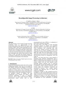
purposes. We refer to this combination of On-The-Fly Computing and Image ..... of the BeBot's camera in a non-deterministic environment, and (ii) the objective.
Towards On-The-Fly Image Processing Alexander Jungmann
Dissertation in Computer Science
submitted to the
Faculty of Electrical Engineering, Computer Science, and Mathematics in partial fulfillment of the requirements for the degree of
doctor rerum naturalium (Dr. rer. nat.)
Paderborn, 2016
Supervisors: Prof. Dr. Franz-Josef Rammig, Paderborn University Prof. Dr. Eyke Hüllermeier, Paderborn University
ii
Abstract Image Processing is fundamental for any camera-based vision system. In order to support the development process of image processing applications, functional prototypes can be realized in advance. Since the entire prototyping process including among others design, realization, functional tests, and evaluation is usually very time-consuming, automating the process to some extend is highly desirable. On-The-Fly Computing, in turn, provides techniques for specifying, composing, executing, and rating functionality. Software components are modeled as services, which encapsulate distinct functionality and can be flexibly combined with each other. The very basic idea of this thesis is to adopt On-The-Fly Computing techniques as foundation for a holistic approach that allows for automated generation of task-specific image processing applications, e.g., for rapid prototyping purposes. We refer to this combination of On-The-Fly Computing and Image Processing as On-The- Fly Image Processing. Throughout this thesis, we gradually develop a holistic, adaptive approach and present concepts for specification, composition, recommendation, execution, and rating of image processing functionality. Image processing applications are realized according to Service-oriented Computing design principles, i.e., distinct image processing functionality is encapsulated in terms of stateless, autonomous services. The proposed specification formalism incorporates a variant of firstorder logic and grounds on domain knowledge provided in terms of ontologies. Complex image processing functionality is defined by the data-flow between input and output ports of services and modeled based on a Petri-net formalism. To automatically compose complex image processing functionality, we present a flexible, Artificial Intelligence planning-based forward search approach, and a multi-step discovery mechanism that gradually reduces valid candidate services for single composition steps. Decision-making between alternative composition steps is supported by a learning recommendation system, which keeps track of valid composition steps by automatically constructing a composition grammar. In addition, it adapts to solutions of high quality by means of feedback-based Reinforcement Learning techniques. For distributed execution of composed services, we propose a message-based Service-oriented Architecture. Since messages include all necessary information, a central controller is not required. Rating mechanisms automatically evaluate the functionality of composed solutions by comparing execution results with desired results, e.g., given in terms of ground truth data. Rating results are used as feedback values for the learning recommendation system. Three concrete use cases with different characteristics are used for motivating and illustrating our proposed concepts. Furthermore, in combination with a prototypical realization, they serve as proofs of concept and demonstrate the feasibility of our holistic approach.
iii
Zusammenfassung Bildverarbeitung ist ein grundlegender Bestandteil jedes Kamera-basierten Systems. Um die Entwicklung von Bildverarbeitungsanwendungen zu unterstützen, können funktionale Prototypen vorab realisiert werden. Eine automatisierte Prototypenentwicklung unter Einbeziehung von Entwurf, Umsetzung, Test und Evaluierung vermag den gesamten Entwicklungsprozess weiter zu beschleunigen. On-The-Fly Computing bietet diesbezüglich allgemeine Techniken zur Spezifikation, Komposition, Ausführung und Bewertung von Funktionalität. Softwarekomponenten werden als Services modelliert und können flexibel miteinander kombiniert werden. Die Grundidee dieser Arbeit ist daher, On-The-Fly Computing Techniken als Fundament für einen ganzheitlichen Ansatz zu nutzen und eine automatische Generierung von Bildverarbeitungsanwendungen zu ermöglichen. Wir bezeichnen diese Kombination aus On-The-Fly Computing und Bildverarbeitung als On-The-Fly Image Processing. In dieser Arbeit werden Konzepte zur Spezifikation, Komposition, Empfehlung, Ausführung und Bewertung von Bildverarbeitungsfunktionalität vorgestellt, und sukzessive ein ganzheitlicher, adaptiver Ansatz entwickelt. Analog zu Service -oriented Computing Gestaltungsgrundsätzen werden einzelne Bildverarbeitungsalgorithmen als zustandslose, autonome Services realisiert und spezifiziert. Der vorgeschlagene Spezifikationsansatz basiert auf einer Variante von Prädikatenlogik. Domänenwissen wird in Form von Ontologien bereitgestellt. Komplexe Bildverarbeitungsfunktionalität wird anhand des Datenflusses zwischen Services definiert und mittels Petri-Netze beschrieben. Eine automatisierte Komposition komplexer Funktionalität wird durch eine flexible Vorwärtssuche ermöglicht. Ein mehrstufiges Verfahren identifiziert und reduziert schrittweise die Menge der Service Kandidaten für einzelne Kompositionsschritte. Die Entscheidungsfindung zwischen alternativen Kompositionsschritten wird durch ein lernendes Empfehlungssystem unterstützt, welches gültige Kompositionsschritte in Form einer Kompositionsgrammatik verwaltet. Um qualitativ hochwertige Lösungen zu identifizieren, wird darüber hinaus die Empfehlungsstrategie des Empfehlungssystems durch den Einsatz von Reinforcement Learning Techniken über die Zeit angepasst. Für die verteilte Ausführung komponierter Services wird eine Nachrichten-basierte Service-orientierte Architektur vorgestellt. Nachrichten enthalten sämtliche Informationen und machen eine zentrale Kontrollinstanz überflüssig. Bewertungsverfahren beurteilen die Funktionalität von komponierten Services anhand konkreter Ausführungsergebnisse. Bewertungswerte fließen anschließend als Feedback in das lernende Empfehlungssystem ein. Konkrete Anwendungsfälle aus drei verschiedenen Problemdomänen dienen zur Veranschaulichung der vorgeschlagenen Konzepte. In Kombination mit einer prototypischen Umsetzung demonstrieren sie zudem die Machbarkeit unseres ganzheitlichen, adaptiven Ansatzes.
iv
Contents 1 Introduction 1.1 On-The-Fly Image Processing . . . . . . . . . . . . . . . . . . . . 1.2 Objectives . . . . . . . . . . . . . . . . . . . . . . . . . . . . . . . 1.3 Outline and Contributions . . . . . . . . . . . . . . . . . . . . . . 2 Preliminaries 2.1 Introduction to Image Processing . . . . . . . . . . . . 2.1.1 Image Manipulation vs. Image Processing . . . 2.1.2 Fundamental Steps in Image Processing . . . . 2.1.3 Real-world Application Scenario . . . . . . . . . 2.1.4 Developing Image Processing Solutions . . . . . 2.2 Introduction to On-The-Fly Computing . . . . . . . . . 2.2.1 Principles of Service-Orientation . . . . . . . . . 2.2.2 Service-Oriented Computing . . . . . . . . . . . 2.2.3 The On-The-Fly Computing Concept . . . . . . 2.2.4 On-The-Fly Composition Process . . . . . . . . 2.3 On-The-Fly Image Processing . . . . . . . . . . . . . . 2.3.1 Principles of Service-oriented Image Processing 2.3.2 Fundamental Challenges . . . . . . . . . . . . . 2.3.3 Adaptivity by Feedback-based Learning . . . . . 2.4 Related Work . . . . . . . . . . . . . . . . . . . . . . . 3 Use Cases 3.1 Data-Flow and Control-Flow . . . . . . . . . . . . . . 3.1.1 Data-Flow Graphs as Execution Model . . . . 3.1.2 Elementary Net Systems based on Petri Nets . 3.1.3 Three Classes of Composed Solutions . . . . . 3.2 Thumbnails for an Online Photo Gallery . . . . . . . 3.2.1 Required Functionality . . . . . . . . . . . . . 3.2.2 Characteristics . . . . . . . . . . . . . . . . . 3.3 Color-based Segmentation . . . . . . . . . . . . . . . 3.3.1 Concrete Context . . . . . . . . . . . . . . . . 3.3.2 Required Functionality . . . . . . . . . . . . . 3.3.3 Characteristics . . . . . . . . . . . . . . . . . 3.4 Motion-based Object Detection . . . . . . . . . . . . 3.4.1 Concrete Context . . . . . . . . . . . . . . . .
. . . . . . . . . . . . .
. . . . . . . . . . . . . . .
. . . . . . . . . . . . .
. . . . . . . . . . . . . . .
. . . . . . . . . . . . .
. . . . . . . . . . . . . . .
. . . . . . . . . . . . .
. . . . . . . . . . . . . . .
. . . . . . . . . . . . .
. . . . . . . . . . . . . . .
. . . . . . . . . . . . .
1 2 3 3
. . . . . . . . . . . . . . .
7 7 8 9 11 15 17 17 19 20 22 25 25 28 32 35
. . . . . . . . . . . . .
39 39 40 43 47 49 50 51 51 51 53 54 54 55
v
Contents
3.5
3.4.2 Required Functionality . . . . . . . . . . . . . . . . . . . . 3.4.3 Characteristics . . . . . . . . . . . . . . . . . . . . . . . . Summary . . . . . . . . . . . . . . . . . . . . . . . . . . . . . . .
4 Symbolic Service Composition 4.1 Knowledge-based Specifications . . . . . . . . 4.1.1 Body of Knowledge . . . . . . . . . . . 4.1.2 Service and Request Specification . . . 4.1.3 Specification Example: Thumbnails . . 4.1.4 Specification Example: Segmentation . 4.2 Planning-based Service Composition . . . . . 4.2.1 Composed Services . . . . . . . . . . . 4.2.2 Body of Rules . . . . . . . . . . . . . . 4.2.3 Formal Framework . . . . . . . . . . . 4.2.4 Composition Algorithm . . . . . . . . . 4.2.5 Composition Example: Thumbnails . . 4.3 Shortcomings and Extensions . . . . . . . . . 4.3.1 Exponentially Growing Solution Space 4.3.2 Incorrect Task Definitions . . . . . . . 4.3.3 Superfluous Search Paths and Services 4.3.4 Discarding Properties of Visual Data . 4.3.5 Outlook: Necessity for Learning . . . . 4.4 Evaluation . . . . . . . . . . . . . . . . . . . . 4.4.1 Prototypical Implementation . . . . . . 4.4.2 Concrete Composition Problem . . . . 4.4.3 Search Space and Solution Space . . . 4.4.4 Time to Solution . . . . . . . . . . . . 4.4.5 Conclusion . . . . . . . . . . . . . . . . 4.5 Related Work . . . . . . . . . . . . . . . . . . 5 Execution and Rating 5.1 Service-oriented Architecture for Execution . . 5.1.1 Key Concepts and Building Blocks . . 5.1.2 Integration into OTF Image Processing 5.2 Problem Domain specific Rating Processes . . 5.2.1 Preliminary Considerations . . . . . . 5.2.2 Segmentation Use Case . . . . . . . . . 5.2.3 Object Detection Use Case . . . . . . . 5.3 Evaluation . . . . . . . . . . . . . . . . . . . . 5.3.1 Segmentation of Color Palette . . . . . 5.3.2 Motion-based Robot Detection . . . . 5.3.3 Motion-based Ball Detection . . . . . . 5.3.4 Conclusion . . . . . . . . . . . . . . . .
vi
. . . . . . . . . . . . . . . . . . . . . . . .
. . . . . . . . . . . .
. . . . . . . . . . . . . . . . . . . . . . . .
. . . . . . . . . . . .
. . . . . . . . . . . . . . . . . . . . . . . .
. . . . . . . . . . . .
. . . . . . . . . . . . . . . . . . . . . . . .
. . . . . . . . . . . .
. . . . . . . . . . . . . . . . . . . . . . . .
. . . . . . . . . . . .
. . . . . . . . . . . . . . . . . . . . . . . .
. . . . . . . . . . . .
. . . . . . . . . . . . . . . . . . . . . . . .
. . . . . . . . . . . .
. . . . . . . . . . . . . . . . . . . . . . . .
. . . . . . . . . . . .
. . . . . . . . . . . . . . . . . . . . . . . .
. . . . . . . . . . . .
. . . . . . . . . . . . . . . . . . . . . . . .
. . . . . . . . . . . .
57 58 59
. . . . . . . . . . . . . . . . . . . . . . . .
61 63 63 70 73 76 79 80 81 83 90 96 100 101 104 106 111 116 117 117 118 120 123 126 127
. . . . . . . . . . . .
135 136 136 140 141 142 144 153 165 165 170 174 176
Contents 6 Adaptive Service Composition 6.1 Learning Recommendation System . . . . . . 6.1.1 Reinforcement Learning . . . . . . . . 6.1.2 Recommendation Model . . . . . . . . 6.1.3 Learning Process . . . . . . . . . . . . 6.2 Combining Composition and Recommendation 6.2.1 Overview and Interactions . . . . . . . 6.2.2 Update Step . . . . . . . . . . . . . . . 6.2.3 Evaluation Step . . . . . . . . . . . . . 6.2.4 Modified Search Node Selection . . . . 6.2.5 Episode Finalization . . . . . . . . . . 6.3 Evaluation . . . . . . . . . . . . . . . . . . . . 6.3.1 Segmentation of Color Palette . . . . . 6.3.2 Motion-based Robot Detection . . . . 6.3.3 Motion-based Ball Detection . . . . . . 6.3.4 Conclusion . . . . . . . . . . . . . . . . 6.4 Related Work . . . . . . . . . . . . . . . . . .
. . . . . . . . . . . . . . . .
. . . . . . . . . . . . . . . .
. . . . . . . . . . . . . . . .
. . . . . . . . . . . . . . . .
. . . . . . . . . . . . . . . .
. . . . . . . . . . . . . . . .
. . . . . . . . . . . . . . . .
. . . . . . . . . . . . . . . .
. . . . . . . . . . . . . . . .
. . . . . . . . . . . . . . . .
. . . . . . . . . . . . . . . .
179 180 181 184 191 195 196 197 205 209 212 213 214 218 223 227 228
7 Conclusion and Outlook 233 7.1 Future Work . . . . . . . . . . . . . . . . . . . . . . . . . . . . . . 235 List of Figures
237
List of Tables
245
List of Algorithms
247
Own Publications
249
Bibliography
253
vii
1 Introduction Image Processing is fundamental for any camera-based vision system that aims for extracting scene-data from images for autonomous, machine-based perception [25]; be it advanced driver assistance systems or even autonomous driving in the automotive domain, quality inspection or general process automation in manufacturing industry, or augmented reality scenarios, where images of the environment are analyzed and augmented by additional information. The functionality of image processing applications, however, heavily depends on the concrete task and has to be optimized according to the underlying conditions. In order to support the development process, functional prototypes can be realized, analyzed, and revised in advance. By doing so, developers can focus on the desired functionality, while determining at an early stage, if and how the underlying image processing task can be solved in the first place. Since the entire prototyping process including design, realization, functional tests, and evaluation is usually very time-consuming, automating the process to some extend is highly desirable. On-The-Fly (OTF) Computing, in turn, provides techniques for specifying, composing, executing, and rating functionality [26]. Software components are modeled as services, which encapsulate distinct functionality and can be flexibly combined with each other. Composed services are executed in a distributed manner. In fact, OTF Computing consequently carries on Service-oriented Computing (SOC) principles such as the automated composition of service-based applications [27]. In the long run, OTF Computing aims for automated composition of customized software solutions based on services that are traded on dynamic markets and can be flexibly combined. While not considering economical aspects, the very basic idea of this thesis is to use OTF Computing techniques as foundation for a holistic approach that allows for automated generation of task-specific image processing applications, e.g., for rapid prototyping purposes [1]. We refer to this combination of OTF Computing and Image Processing as OTF Image Processing.
1
1 Introduction
1.1 On-The-Fly Image Processing The starting point for OTF Image Processing is to interpret image processing algorithms as services; that is, to design image processing services based on existing algorithms while adhering to common SOC design principles [28]. In order to automatically generate service-based image processing applications, OTF Computing techniques shall be applied. In our opinion, both domains benefit from this connection. On the one hand, interpreting image processing algorithms as services and automatically composing image processing services according to the OTF Computing paradigm constitutes both a sound and promising starting point for automatically composing image processing applications in general. On the other hand, concrete examples from the image processing domain enable us to investigate and clarify open challenges in the OTF Computing domain (and in the SOC domain in general) as well as to develop and evaluate new methods in order to meet these challenges. From the image processing perspective, we investigate to what extent service composition techniques facilitate automatic composition of image processing functionality and how to overcome possible shortcomings. In doing so, we obtain new insights in a domain with specific characteristics. This, in turn, enables us to come up with more specialized concepts. These concepts can then be generalized and transferred back to the SOC domain in the long run. From the SOC perspective, the characteristics of the image processing domain such as �
high variability of existing services in terms of traditional algorithms,
�
demand for composed services providing task-specific functionality,
�
availability of executable implementations provided by open source libraries,
�
inherent vividness for motivating new challenges and new concepts,
enable us to realize examples of highly practical relevance, while the complexity of those examples can be gradually increased. In our experience, increased practical relevance has a highly positive impact on the awareness and acceptance of SOC techniques in general.
2
1.2 Objectives
1.2 Objectives In the most general sense, the objective of this thesis is to gradually develop a holistic yet flexible approach that facilitates automatic composition and execution of image processing functionality. More concretely, the intended approach shall provide means for solving the following tasks: 1. Manual specification of image processing functionality, both for available functionality in terms of services and required functionality in terms of requests. 2. Automatic composition of complex image processing functionality based on available services and according to a specified request. 3. Automatic and distributed execution of composed, service-based image processing functionality. 4. Automatic rating of composed services in order to estimate the discrepancy between required functionality and concrete functionality (i.e., the functionality when processing task-specific input data). 5. Incorporation of rating results as feedback into the composition process in order to adapt decision-making and reduce functional discrepancy over time. The entire approach shall ground on a sound formal basis that facilitates future extensions and modifications. For evaluation, a prototypical implementation combined with different application scenarios shall serve as proof of concept.
1.3 Outline and Contributions Let us briefly summarize each of the upcoming chapters with respect to content and contributions.
Chapter 2: Preliminaries Section 2.1 introduces Image Processing in more detail. It also covers relevant parts of our previous work in this domain. Section 2.2 focuses on the SOC paradigm in general, and – according to our previous work – OTF Computing in
3
1 Introduction particular. The result of this section is a fundamental OTF Computing framework, which serves as guideline for the work at hand. Section 2.3 finally presents our novel idea of OTF Image Processing in more detail and sets the stage for all subsequent chapters. This section particularly emphasizes the necessity for Machine Learning techniques in order to achieve a composition process, which is not only automated, but adaptive as well. Section 2.4 discusses work that is related to automated generation of image processing solutions.
Chapter 3: Use Cases In Section 3.1, we describe our Petri-net based approach for modeling data-flow of services and composed services. In fact, when talking about composed image processing functionality, we always refer to data-flow nets, which define image processing functionality in terms of data-flow between service ports. Section 3.2 Section 3.4 subsequently introduce three concrete use cases that are derived from our previous work and accompany us throughout this thesis. Each use case defines a different composition task, as summarized in Section 3.5. Developing new image processing applications, however, is beyond the scope of this thesis.
Chapter 4: Symbolic Service Composition Section 4.1 presents our knowledge-based approach for flexibly specifying image processing functionality in terms of input and output data as well as image processing tasks. The specification approach bases on ontologies for modeling domain knowledge, and incorporates a variant of first-order logic for the actual specification formalism. Please note that, although the specification approach actually allows for specifying image processing functionality on different levels of abstraction, we mainly focus on the lowest level in the subsequent sections and chapters. Section 4.2 introduces our composition approach that realizes a planning-based forward search algorithm as well as a multi-step service discovery mechanism in order to compose image processing functionality based on service and request specifications. Section 4.3 points out remaining shortcomings of the composition approach. Furthermore, it proposes modifications that are either optional or mandatory in order to solve the composition tasks defined by our use cases. One of the use cases is subsequently used in Section 4.4 as concrete application scenario for evaluating the heretofore introduced composition approach. Section 4.5 finally
4
1.3 Outline and Contributions discusses work that is related to automatic service composition.
Chapter 5: Execution and Rating Section 5.1 describes our service-oriented architecture for execution of composed services. In our previous work, it was successfully applied in a robotics context for outsourcing computationally expensive functionality. It is perfectly suited for automated execution of composed image processing functionality, and can be easily integrated into the overall framework. Section 5.2 introduces use case specific rating mechanisms for automatically quantifying the discrepancy between required functionality and concrete functionality given concrete execution results and – among others – pre-defined ground truth data. The rating mechanisms are subsequently evaluated in Section 5.3.
Chapter 6: Adaptive Service Composition Section 6.1 introduces our so called learning recommendation system, which – in combination with the composition algorithm – facilitates adaptive service composition. By automatically constructing and maintaining a composition grammar, the recommendation systems keeps track of valid composition steps identified by the composition algorithm. To achieve adaptivity, the sequential selection of valid composition steps is modeled as Markov Decision Process and tackled by Reinforcement Learning techniques. Feedback is provided by the previously mentioned rating mechanisms. Section 6.2 describes the message-based interaction of composition algorithm and learning recommendation system, as well as necessary adjustments to be made to the composition algorithm. The entire approach including composition, execution, rating, and learning is subsequently evaluated in Section 6.3. In this context, please note that optimizing the learning behavior of the applied learning techniques or developing new learning techniques is beyond the scope of the work. Section 6.4 finally discusses work that is related to adaptive service composition.
Chapter 7: Conclusion and Outlook Chapter 7 concludes the work at hand and summarizes major loose ends, which – in our opinion – represent the most reasonable starting points for future work.
5
2 Preliminaries This chapter serves as an informal introduction of the fundamental scope of this thesis, motivates the idea of On-The-Fly Image Processing in more detail, and serves as basis for all following chapters. Section 2.1 gives a general introduction to Image Processing and motivates the automated generation of image processing applications. Section 2.2 introduces On-The-Fly Computing and its relationship to Service-oriented Computing. Furthermore, it derives a basic framework for all following considerations. Finally, Section 2.3 explicitly connects Image Processing with On-The-Fly Computing, motivates the benefits of this connection from both the Image Processing perspective and the On-The-Fly Computing perspective, and sets the stage for the remainder of this work.
2.1 Introduction to Image Processing Image Processing addresses two principal applications areas: improvement of visual information for human interpretation (also referred to as image manipulation), and extraction of scene data for autonomous, machine-based perception [25]. In the most general sense, both application areas usually incorporate multiple data processing steps. A single processing step can be applied, e.g., to produce a modified version of an image (e.g., by scaling or color adjustments), or to extract task-specific information from an image. In any case, the starting point for any image processing application are images such as photos, or frames from videos and live camera streams, respectively. In this context, an image I corresponds to a two-dimensional, ordered matrix of integers [29]. More formally, an image I is a two-dimensional function of integer coordinates N × N, mapping to a range of possible (pixel) values P, such that I(u, w) ∈ P and u, w ∈ N.
7
2 Preliminaries The size of an image is determined by its width M (number of columns) and its height N (number of rows). For addressing a pixel P ∈ P at position (u, w) with u ∈ [0, M − 1] and w ∈ [0, N − 1], the following coordinate system is imposed: The origin (0, 0) lies in the upper left corner, the x-axis runs from left to right, and the y-axis runs from top to bottom. The information embedded in a pixel depends on both the data type used to represent it and the type of the image itself. For example, a grayscale image consists of a single channel, which represents the intensity of the image and typically uses 8 bits per pixel value, where 0 corresponds to the minimum brightness (black) and 255 corresponds to the maximum brightness (white). An image in RGB format, in turn, consists of three channels (red, green, blue) to encode color information. Each of the channels makes use of 8 bits, resulting in 3 × 8 = 24 bits to encode the color information of a single pixel.
2.1.1 Image Manipulation vs. Image Processing Software for imaging has been targeted at either manipulating or processing images, either for practitioners and designers (henceforth referred to as users) or software programmers (henceforth referred to as developers), with quite different requirements. Monolithic software packages for manipulating images, such as Adobe Photoshop, Corel Photo-Paint and GIMP, usually offer a convenient user interface and a large number of readily available functions and tools for working with images interactively. In contrast, image processing software primarily aims at the requirements of algorithm and software developers working with images, where interactivity and ease of use are originally not the main concerns. Instead, these environments mostly offer comprehensive and well-documented software libraries that facilitate the implementation of new image processing algorithms, prototypes and working applications. Popular examples are OpenCV [30], ImageMagick [31], and the Image Processing Toolbox from MatLab [32]. In practice, however, image manipulation and image processing are closely related. On the one hand, although Photoshop, for example, is aimed at image manipulation by non-programmers, the software itself implements many traditional image processing algorithms. On the other hand, many of the effects achieved by monolithic software packages can also be achieved by exploiting existing software libraries and implementing appropriate image processing algorithms. In fact, im-
8
2.1 Introduction to Image Processing age processing is at the base of any image manipulation software by providing the building blocks in terms of algorithms.
2.1.2 Fundamental Steps in Image Processing Software solutions for performing specific image processing tasks highly depend on the task-specific problem domain. The fundamental steps, however, are usually very similar. Based on the work of Gonzales and Woods [25], we classify these steps as follows: 1. Image Acquisition: The very first step is responsible for acquiring an image and providing it to the subsequent steps. For example, an image can be obtained by loading the content of a single image file, by extracting the next frame from a video file, or by grabbing a frame from a camera. We refer to an acquired image that was not modified at all as original image. 2. Preprocessing: In the most general sense, the preprocessing step is responsible for improving the original image in order to increase the chances for success of the subsequent steps. That is, acquisition defects such as compression artefacts, image noise, or lense distortion are reduced. For example, preprocessing may involve contrast enhancement or noise reduction. As output, the preprocessing step provides a modified version of the original image. We generally refer to this image as preprocessed image. 3. Segmentation: Roughly speaking, the segmentation step reduces the visual information embedded in an image to the actually relevant information by partitioning an image into its constituent parts or visual primitives such as points, lines, contours, or areas [33]. The type of visual primitives to be identified as well as the level to which the subdivision of the image is carried depends on the problem to be solved. The output of this step usually is raw pixel data, constituting, e.g., the boundaries of a visual primitive or all pixels related to a visual primitive. The data type of the output, however, is not necessarily an image anymore, but can be, e.g., a plain list of pixel values, or a run-length encoded set of coordinates [34]. Either case, since a single visual primitive can generally be considered as a region of pixels (set of coordinates) in the image plane, we refer to the output of the segmentation step as regions.
9
2 Preliminaries problem domain
Image Acquisition
original image
Preprocessing
preprocessed image
Segmentation
regions (raw pixel data) Representation and Description
regions (features)
Recognition and Interpretation
objects
Figure 2.1: Fundamental steps in image processing. 4. Representation and Description: After identifying relevant information in terms of regions, a more suitable representation and description for subsequent computer processing is required. First, a decision whether the data should be represented as a boundary or a complete region has to be made. While a boundary representation emphasizes shape characteristics, the representation as complete region emphasizes internal properties such as texture. If required, both representations are combined though. Second, a method for describing the data so that features of interest are highlighted has to be specified. This so called feature selection process deals with extracting features that result in some quantitative information that is basic for differentiating one class of regions from another. 5. Recognition and Interpretation: The last step involves recognition and interpretation. Recognition (or classification) is the process that assigns a label to a region based on the information provided by its features. Interpretation involves assigning meaning to an ensemble of previously recognized regions. We also refer to this last step as object detection. In the most general sense, the result of this step is a set of objects that is used by subsequent decision-making processes beyond image processing. Figure 2.1 shows both the introduced image processing steps and the corresponding input and output data, respectively. The additionally annotated problem domain represents the task-specific overall setting, which comprises, e.g., the context of the image acquisition step and the actual objective that has to be solved. The mutual task of all steps is to gradually reduce and abstract the visual information embedded in the original image in order to extract the visual information that is actually relevant for the problem domain.
10
2.1 Introduction to Image Processing
LED dome
Finish
Pylone
Ball
Camera
BeBot Pylone
Differential chain drive
Passive gripper
(a)
(b)
Figure 2.2: Real-world application scenario from the robotics domain: A miniature robot BeBot (a) has to autonomously push a ball through a slalom course (b).
2.1.3 Real-world Application Scenario Figure 2.2b shows the schematic view of a real-world application scenario from the robotics domain. In this scenario, a miniature robot BeBot [2] (cf. Figure 2.2a) has to autonomously push a single-colored ball through a slalom course. The course itself consists of small pylones that are arranged in a straight line. A unicolored marker represents the finish of the course. The problem domain of the actual image processing task comprises (i) the image capturing process by means of the BeBot’s camera in a non-deterministic environment, and (ii) the objective to identify the scenario-specific objects (pylones, ball, marker) in the captured images. For solving the image processing task, we applied a flexible approach that supports alternative realizations of the previously introduced fundamental image processing steps [3]. We now describe two of these alternative solutions. Image Processing Solution I Figure 2.3 shows the sequence of image processing steps of the first solution. Figures 2.4a - 2.4d show intermediate results produced by these steps. The original image shown in Figure 2.4a represents a BeBot’s typical subjective view of the scenario setup. After grabbing an image, a color-based segmentation algorithm labels adjacent pixels of similar color as a single region [4]. Regions and their associated pixels are interpreted as two-dimensional Gaussian distributions in the image plane. The spatial information of each region is described in terms of statistical parameters, i.e., in terms of discretized moments [35]. The color
11
2 Preliminaries
BeBot Camera
color image
Color-based Segmentation
adjacent pixels of similar color
Moment Computation
discretized moments, average color
Color-based Classification
discretized moments, color class
Object Detection
ball, pylones, marker
Figure 2.3: Image processing steps of solution I. Nodes and edges with thick border represent parts that differ from solution II (cf. Figure 2.5). information of a region is equivalent to the average color of all associated pixels. Figure 2.4b shows the corresponding intermediate result. The immediate result of the segmentation algorithm is represented by adjacent pixels with identical color values. The regions’ associated features (moments and average color) are represented by image ellipses [36] and by the pixel values themselves. Regions are subsequently classified based on their color information and according to predefined color classes (cf. Figure 2.6a). Figure 2.4c shows the result. Ellipses of regions that could not be assigned to any class at all are still black, whereas ellipses of regions that belong to the same color class have identical color. In the final step, regions belonging to the same class are composed based on their spatial information in order to identify scenario-specific objects (cf. Figure 2.4d). For a heuristical approach, geometric attributes such as mass, center of mass, bounding box, or the previously mentioned image ellipse can be directly derived from the discretized moments. Image Processing Solution II Figure 2.5 shows the sequence of image processing steps of the second solution. Nodes and edges with thick border represent the part of the approach that differs from the first solution; either with respect to the implementation of a single step or with respect to the overall composition. Both the image acquisition step and the object detection step are identical to the corresponding steps in the first solution. That is, neither their implementation nor their position in the execution sequence changed. The steps in between, however, were modified. The segmentation algorithm now incorporates a classification mechanism based
12
2.1 Introduction to Image Processing
(a)
(b)
(c)
(d)
Figure 2.4: Intermediate results of the image processing steps shown in Figure 2.3: (a) original color image, (b) regions as adjacent pixels of similar color with raw pixel and feature-based representation, (c) classified and unclassified regions, (d) detected objects.
on color classes. Figure 2.6a shows exemplary color classes defined as distinct subspaces in the RGB color space. Pixels are assigned to a color class if their values are located within such a subspace. Adjacent pixels belonging to the same color class are then assigned to the same region. In other words, the criteria of homogeneity for determining whether adjacent pixels belong to the same region switched from “similar color” to “same color class”. Pixels that cannot be assigned to any color class are considered to be irrelevant and are directly discarded. That is, only visual information that is actually relevant for the problem domain is extracted. As a consequence, the amount of regions produced by the segmentation algorithm is significantly reduced in comparison to the segmentation algorithm in the first solution (cf. Figure 2.4b vs. Figure 2.6b). After identifying relevant regions and assigning them to a color class, moments are computed. This step implements exactly the same method as in the first solution. A subsequent classification step, however, is obsolete. Instead, the object detection step immediately follows.
13
2 Preliminaries color image
BeBot Camera
Segmentation based on Color Classes
adjacent pixels of same color class discretized moments, color class
Moment Computation
Object Detection
ball, pylones, marker
Figure 2.5: Image processing steps of solution II. Nodes and edges with thick border represent parts that differ from solution I (cf. Figure 2.3).
(a)
(b)
Figure 2.6: (a) Color classes are subspaces in the underlying RGB color space. (b) Intermediate results of the image processing solution shown in Figure 2.5 after segmentation and computation of moments. Conclusion While both presented image processing solutions indeed represent concrete instantiations of the introduced fundamental image processing steps, they also reveal that these fundamental steps are rather a rough classification than a strict framework. A separate preprocessing step, e.g., is completely neglected in both approaches. In fact, preprocessing mechanisms are directly integrated into the segmentation algorithm in order to minimize redundant processing steps. The second solution even further reduces redundant processing steps by incorporating a classification mechanism directly into the segmentation algorithm and discarding irrelevant visual information already on pixel level: Pixels that do not belong to a predefined color class are not considered in the segmentation process in the first place. As shown in our previous work [3], this integrated approach
14
2.1 Introduction to Image Processing significantly reduces the execution time for image processing. The drawback, however, is the decreasing robustness in the face of a non-deterministic environment. If, e.g., the lighting conditions change, the pixel values change as well. The predefined color classes, however, are static. As a consequence, a pixel that was previously assigned to a color class, may be considered to be irrelevant in an image captured under different lighting conditions. In this respect, the first solution is more robust. It does not compare pixel values absolutely based on color classes, but relatively based on color similarity. Furthermore, the likelihood of a region’s average color to be correctly assigned to the according color class is higher, since the averaging mechanism compensates changing lighting conditions to a specific degree.
2.1.4 Developing Image Processing Solutions In general, when facing a distinct image processing task, a developer has to come up with a solution that �
copes well with acquisition defects such as compression artefacts, image noise, or imbalanced illumination,
�
identifies and extracts relevant visual information while simultaneously rejecting redundant visual information,
�
transforms relevant information into a more convenient but also more abstract representation without loosing important characteristics.
However, as indicated in the previous section, developing image processing solutions heavily depends on the area of application and the underlying conditions. In embedded systems, e.g., image processing software is usually optimized for specific hardware while the implemented algorithms are often highly specialized for certain tasks. In order to reduce redundant implementation steps, a functional prototype can be realized in advance. In doing so, developers primarily focus on the desired functionality. They determine at an early stage, if and how the underlying image processing task can be solved in the first place. A possible way of solving an image processing task is to follow a componentbased approach. Existing algorithms are considered to be distinct components. Components are interconnected in a loosely coupled manner in order to generate a composition of image processing algorithms. A composition is subsequently
15
2 Preliminaries executed and evaluated in an application specific test case. If the evaluation result does not satisfy the requirements, the respective composition is partially refined by adding, removing or adjusting available components. The modified composition is again executed and evaluated. These steps are repeated until either a prototype that provides the desired functionality was realized, or until the task itself is modified, since no feasible solution could be found. In the domain of photo and video post-processing (image manipulation domain), users do not implement a complete post-processing approach by programming new software. They use existing algorithms that are provided by monolithic solutions, such as Adobe Photoshop, Corel Photo-Paint and GIMP, or by webbased solutions (like, e.g., Instagram [37]) and combine them in an arbitrary order. Users, whether or not being an expert, however, follow a strategy that is similar to the previously outlined way of prototyping. In order to get a solution that satisfies the requirements, existing algorithms are consecutively applied in a trial and error manner. Dependent on a user’s degree of expertise, this trial and error process can be highly time consuming. Consider, e.g., a user, who has a concrete idea of how his holiday photos should look like. If he is a novice, however, he has no idea about what algorithms he has to apply to achieve the desired result. As a consequence, he simply tries different algorithms or combinations of algorithms in order to come up with a satisfying result. But even being an expert in image processing does not necessarily mean that you are able to come up with a satisfying solution from scratch. In any case, a composition of concrete algorithms has to be identified, most likely by a trial and error like strategy under context-specific conditions. Regardless of whether being an expert or a novice, developers and users almost always have to deal with one and the same question: Which composition of available algorithms solves the image processing task as good as possible? Automating the Composition Process of Image Processing Solutions By automating the composition of image processing solutions, both developers and users can be supported and the effort for finding a satisfying solution can be minimized. In the best case, an optimal solution that perfectly satisfies all requirements is identified and the problem is solved fully automatically. However, developers and users can even benefit from non-optimal solutions: An automatically composed solution can be used as starting point for manual modifications
16
2.2 Introduction to On-The-Fly Computing while the search space for possibly promising modifications was reduced. The composition process can be supported by providing representative data from the problem domain during the development phase. That is, decision-making during the composition process is supported in terms of more specific information about the problem domain. In this context, representative data can either be concrete images or abstract descriptions of images (e.g., in terms of features). If representative images are available, a partially composed image processing solution can already be executed during the composition process. The intermediate execution result can then be evaluated in order to support decision-making for the next processing step. Last but not least, by deferring decision-making into the actual execution phase during productive operation, appropriate solutions can even be determined justin-time according to the concrete execution context. Consider, e.g., our application scenario. By analyzing original images over time (while the robot is already performing its task), varying illumination conditions can be recognized. Based on the outcome of this analysis, the image processing workflow can be reconfigured (e.g., by incorporating additional preprocessing steps) in order to adapt to varying conditions. In contrast to just adapting parameters of a running application, the application logic itself is changed during execution.
2.2 Introduction to On-The-Fly Computing Software developer have to increasingly face up to the paradigm shift from the principle of purchasing software as monolithic software packages to the principles of SOC [38], which shall enable purchase and execution of distributed software components (services) on demand. OTF Computing intends to drive this paradigm shift forward [26, 39]. This chapter starts with an introduction of fundamental SOC concepts. Afterward, the OTF Computing concept and its relationship to SOC are described, and a framework as basis for the remainder of this thesis is derived.
2.2.1 Principles of Service-Orientation Service-orientation is said to have its roots in a software engineering theory known as “separation of concerns” [27]. The theory states that it is beneficial to break
17
2 Preliminaries down a large problem into a series of individual concerns. This allows the logic required to solve the problem to be decomposed into a collection of smaller, related pieces. Object-oriented programming and component-based programming approaches, e.g., achieve a separation of concerns by using objects, classes, and components, respectively. Service-orientation, in turn, achieves a separation of concerns by means of services. Each service addresses a specific concern, while the design of services adheres to the service-orientation design paradigm providing the following set of design principles [28]: Reusability: Regardless of whether immediate reuse opportunities exist, services are designed to support possible reuse. Formal contract (description): For services to interact, they need not share anything but a formal contract that describes each service and defines the terms of information exchange. Loosely coupling: Services must be designed to interact without the need for tight, cross-services dependencies. Abstraction: The only part of a service that is visible to the outside world is what is exposed via its description. Underlying logic and implementation details are invisible and irrelevant to service requestors. Composability: A service may be composed of other services. This allows logic to be represented at different levels of granularity and promotes reusability. Autonomy: The logic governed by a service resides within an explicit boundary. The service has control within this boundary and is not dependent on other services for it to execute its governance. Statelessness: Services should not be required to manage state information, as that can impede their ability to remain loosely coupled. Services should be designed to maximize statelessness even if that means deferring state management elsewhere. Discoverability: Services should allow their descriptions to be discovered and understood by service requestors that may be able to make use of their logic.
18
2.2 Introduction to On-The-Fly Computing Service-Oriented Architecture is primarily distinguished by
is designed to support the implementation of Service-Orientation
Design Paradigm provides principles that shape the design of
Services
is designed to support the implementation of
provides principles that shape the design of are composed of is comprised of
is designed to support the creation and evolution of a
Composed Services
draw from the
Service Inventory
can be comprised of
Service-Oriented Solution Logic is comprised of standardized
Figure 2.7: SOC elements and their relations [40].
2.2.2 Service-Oriented Computing SOC represents a new generation distributed computing platform [40]. It is a cross-disciplinary paradigm for distributed computing that gradually changes the way software applications are designed, delivered and consumed. Metaphorically speaking, the term SOC can be considered as a big umbrella, which encompasses past distributed computing platforms, while adding new design layers, governance considerations, and a vast set of preferred implementation technologies. Figure 2.7 shows the SOC key elements and how each element ties into others. To sum it up in one sentence, service-oriented architecture represents a distinct form of technology architecture designed in support of service-oriented solution logic which is comprised of services and composed services designed according to the service-orientation design paradigm and assembled in one ore more service inventories. More concretely: �
Service-oriented solution logic is implemented as services and composed services, and designed in accordance with the previously introduced design principles.
�
A composed service is composed of services that have been interconnected to provide the functionality required to automate a specific task or process.
19
2 Preliminaries
Request
Dynamic Market of Services
... OTF Provider
Customer
Service Provider
Service Provider Service Provider
Response
Figure 2.8: On-The-Fly (OTF) Computing: A so-called OTF provider receives and processes a customer’s request. �
One service may be invoked by multiple applications, each of which can incorporate that same service in different composed services.
�
A collection of standardized services can form the basis of a service inventory that can be administered independently.
�
Processes can be automated by the creation of composed services that draw from a pool of existing services assembled in a service inventory.
�
Service-oriented architecture is a form of technology architecture optimized in support of services, composed services, and service inventories.
Creation of composed services can be either accomplished by hand – based on expertise and experience – or automatically. Automation of this service composition process, however, is a formidable challenge: Functional as well as non-functional requirements have to be satisfied.
2.2.3 The On-The-Fly Computing Concept A major goal of the OTF Computing project is the automated composition of customized software solutions based on services that are traded on dynamic markets and that can be flexibly interconnected with each other [5]. According to the vision of OTF Computing, a user (henceforth referred to as customer) formulates a request for a customized software solution, receives a response in terms of a composed service, and finally executes the composed service. Figure 2.8 illustrates the very basic idea of OTF Computing. A so-called OTF provider receives
20
2.2 Introduction to On-The-Fly Computing and processes a customer’s request. The processing step mainly involves automatic composition of customized software solutions based on services supplied by service providers. The OTF provider responds in terms of a composed service that satisfies the requirements specified in the customer’s request. Figure 2.9 gives a very abstract overview of the OTF Computing concept. In the most general sense, it can be divided into three main layers, each of them realizing distinct functionality and dealing with a different amount of services. The upper layer represents the global market of services. It includes without limitation market mechanisms for trading in services as well as algorithms for discovering and matching services in a network. The lower layer comprises an extensive verification step of composed services regarding functional as well as non-functional properties and requirements. Furthermore, the lower layer provides necessary means for executing the established compilation of services. The middle layer realizes the actual service composition process. It is the connection link between upper and lower layer. It interacts with the upper layer to retrieve candidate services from the global market and passes a composed service to the lower layer for verification and execution. The OTF Computing concept is closely related to the SOC paradigm. In fact, the entire OTF Computing concept can be considered as a distinct form of serviceoriented architecture. Software components are designed as services according to the principles provided by the service-orientation design paradigm. Services are formally described by means of functional and non-functional properties [41, 42]. Based on their descriptions, services can be interconnected in a loosely coupled manner to build composed services for solving more complex tasks [6]. The OTF Computing market of services fulfills the function of a service inventory. Services, however, are not assembled in a central repository, but supplied by independent service providers that are distributed across a dynamic market
Candidate Services Composed Service
Discovery and Matching in a Dynamic Market of Services Composition, Rating, and Evaluation
Decreasing number of services.
Verification and Execution
Figure 2.9: Abstract overview of the OTF Computing concept.
21
2 Preliminaries
3) Execution
1) Request
OTF Provider Selection
OTF Provider
Service Discovery
Service Composition
Service Provider Selection
2) Response Service Provider 4) Rating Customer
Service Recommendation
Service Matching
Figure 2.10: The OTF service composition process in the market environment. environment. Service providers may change their service repertoire by offering new services, removing old services, or updating existing services. Furthermore, service providers may either enter the market as new participants or completely leave the market. From an OTF provider’s perspective the complete set of all available services is not known at any time, but can only be partially discovered just in time [7].
2.2.4 On-The-Fly Composition Process Figure 2.10 shows the OTF Computing process and its relevant subprocesses. Three different classes of market participants are involved in the overall process: customers, OTF providers, and service providers. In this context, OTF Provider Selection and Service Provider Selection are reputation-based decisionmaking processes regarding transactions between these market participants [8, 9]. A customer formulates a request for an individual software solution and sends the request to an OTF provider of his choice (Step 1). The selected OTF provider processes the request and automatically composes a solution based on services that are supplied by independent service providers. In the most general sense, the Service Composition process is interpreted as sequential application of composition steps. A composition step may, e.g., correspond to selecting a service in order to realize a placeholder within a workflow [43, 44]. A composition step, however, may also correspond to a single step within a composition algorithm based on Artificial Intelligence (AI) planning approaches [45–48]. Either case, similar to a customer’s request, an OTF provider formulates a request according to the requirements of the current composition step and asks a selected subset of service providers for appropriate services. Processing the response of a service provider is divided into two separate pro-
22
2.2 Introduction to On-The-Fly Computing cesses. By doing so, the amount of qualified candidate services is gradually reduced. First of all, a Service Matching process determines to what extent a particular service fulfills the functional (e.g., signatures and behavior) as well as non-functional requirements (e.g., quality properties such as response time or reliability) that are specified in the OTF provider’s request [49, 50]. Based on the matching result, services that provide significantly different functionality or that violate important non-functional restrictions are directly discarded. The matching process is part of the OTF Computing architecture and takes place before an OTF provider receives a response about appropriate candidate services. Put another way, the matching process operates as a filter ensuring that only services that fulfill the desired requirements to a certain extent are returned. After the matching process, a Service Recommendation process identifies and ranks the best candidate services out of the set of remaining services [10, 11]. In comparison to the matching process, the recommendation process is part of the OTF provider-specific composition process and highly depends on the context of the request. That is, explicitly given non-functional objectives [12] (e.g., maximizing the performance while simultaneously minimizing the costs) as well as implicit knowledge from previous composition processes [13] (e.g., a certain service is more qualified in a particular context than others) are considered. As soon as a composed service is completed, it is passed on to the customer (Step 2), who subsequently executes it (Step 3). The customer rates his degree of satisfaction regarding the quality of the execution result (Step 4). The rating value is returned as feedback value to the associated OTF provider. Based on the feedback value, the OTF provider then adjusts its recommendation strategy in order to improve the quality of future composed services [14, 15]. Basic Framework - A More Technical Perspective We now break down the entire OTF Computing process into a basic framework. Figure 2.11 shows the OTF Computing process from a more technical perspective including all components and processes that are relevant for the work at hand. This framework serves as reference for the remainder of this work. For the time being, the entire process is divided into three consecutive phases: composition, execution, and rating. Composition phase: A (human or artificial) requestor formulates a request that abstractly represents the actually desired functionality in terms of a formal
23
2 Preliminaries Loop Request Composition Phase
Composition
Discovery Candidate Services
Requestor
Execution Phase
Discovery Request
Requ ester
Composed Service Data
Execution Execution Result
Rating Phase
Feedback Rating
Figure 2.11: Basic OTF Computing framework.
specification. The composition process iteratively constructs a composed service based on formal service descriptions. Each iteration includes discovering candidate services for realizing a part of the specified functionality. Candidate services are provided by a non-deterministic discovery mechanism. That is, we assume identical discovery requests to result in different sets of candidate services over time. Furthermore, the discovery mechanism operates in an online manner. That is, available candidate services cannot be discovered in advance (offline), but have to be discovered on-demand based on a request.
Execution phase: After composing a solution, the execution phase takes place. The composed service is executed based on concrete data provided by the requestor. The execution result can either be concrete output data or a concrete behavior of a system.
Rating phase: In the composition phase, a solution that is valid with respect to a formally but abstractly specified functionality is composed. Executing the composed service produces a concrete functionality in terms of output data or system behavior. To quantify the quality of the concrete functionality, the execution result is evaluated in a rating process. The rating value is then used as feedback value in a feedback loop for improving the composition process over time.
24
2.3 On-The-Fly Image Processing
service s3 service s1 image width
image
(a)
service s2 image x scale
image
(b)
image width
image
height
(c)
Figure 2.12: Black box view on image processing services s1 , s2 , and s3 , each implementing a different functionality for image resizing.
2.3 On-The-Fly Image Processing As the name implies, the major idea behind OTF Image Processing is to connect Image Processing with OTF Computing. That is, in order to automatically generate image processing solutions, OTF Computing techniques shall be applied.
2.3.1 Principles of Service-oriented Image Processing The starting point for OTF Image Processing is to interpret image processing algorithms as services; that is, to design image processing services based on existing image processing algorithms and according to the SOC design principles. Elementary Services In OTF Computing and so in this thesis, we consider elementary services (also simply referred to as services) to be black boxes that are described based on their inputs and outputs. Neither implementation details nor internal behavior are visible. As an example, Figure 2.12 shows three different elementary services that all provide functionality for image resizing. We graphically represent such a service as a component with input ports and output ports. For the time being, the annotations are rather informal to illustrate the basic concept of image processing services. If data is provided at each input port, the service consumes the input data, produces new data according to the implemented functionality, and puts the new data into the corresponding output ports. Service s1 requires as input data the actual image that shall be resized as well as the width of the desired size. If we were able to look into the internal behavior of the service, we would see that the height of the output image is calculated automatically according to the ratio of the original width and desired width. With-
25
2 Preliminaries
(a)
(b)
(c)
Figure 2.13: (a) Original image was resized while preserving the original aspect ratio (b) and while ignoring it (c). out a more detailed specification regarding input and output behavior, however, there is no way to have this knowledge in advance. That is, without additional information, we do not know whether service s1 resizes the photo depicted in Figure 2.13a while preserving the aspect ratio (cf. Figure 2.13b) or whether service s1 just simply modifies the width and completely ignores the image height (cf. Figure 2.13c). Service s2 is quite similar to service s1 , except that s2 requires a relative value (a scale factor) for modifying the width of the original image. Again, however, without more information about how the service defines the height of the new image, we cannot foresee whether executing the service changes the original aspect ratio or not. In comparison to services s1 and s2 , service s3 provides a more basic functionality. That is, in addition to the actual image to be resized, s3 requires absolute values for the desired width and the desired height. Whether the aspect ratio is preserved or not completely depends on the input values. As a consequence, both s1 and s2 can be realized in terms of composed services that incorporate s3 . Composed and Configured Services Figure 2.14 shows service s1 as composed service, consisting of elementary services s3 , s4 , s5 , and s6 . Since service s1 was composed, a white box view on its internal behavior is available. That is, its building blocks in terms of elementary services as well as the data flow in terms of port interconnections between these services are visible. The elementary services, in turn, are black boxes. Within the context of composed service s1 , 1. service s4 determines the size in terms of width and height of the input
26
2.3 On-The-Fly Image Processing service s1 service s6
service s4 image
image
width
height width
service s5 x y
x/y
x y
x·y
service s3 image height image
image
width
Figure 2.14: White box view on service s1 as a composed service. image, 2. service s5 calculates the scaling factor based on the width of the input image and the desired width, 3. service s6 calculates the new height based on the scaling factor and the height of the input image, and 4. service s3 finally resizes the input image according to the desired width and the calculated height. To sum it up, composed service s1 adjusts the width of an input image according to a desired width, while preserving the aspect ratio of the input image. We refer to services that are building blocks of a composed service and whose input and output ports are set up for interaction within the context of a composed service as configured services. In case of composed service s1 , services s3 , s4 , s5 , s6 are configured services. The data flow is defined by the port interconnections. In case of composed service s1 , the data flow also directly implies the control flow in terms of the execution sequence [s4 , s5 , s6 , s3 ]. Figure 2.15 shows another example for a composed service that incorporates service s3 , but only service s3 . In this context, s3 was configured during the composition process to resize any input image to a fixed width (320) and height (240). That is, service s7 only requires the image to be resized as input. Statelessness The majority of traditional image processing algorithms is stateless from scratch. For example, a postprocessing algorithm usually consumes an image and produces a modified version of that image without relying on any state information or
27
2 Preliminaries information from previous execution processes. Furthermore, algorithms such as tracking algorithms that depend on historical data can be designed as stateless services by providing historical data as input values. In fact, image processing algorithms usually are non-interactive, data-processing subprocesses of a superior image processing application. All data for such a subprocess can be provided as input values. As a consequence, we assume image processing services to be stateless in general. Autonomy The behavior of many image processing algorithms can be influenced by adjusting algorithm-specific parameters. For example, the color-based segmentation algorithm that was mentioned in Section 2.1.3 uses color similarity as criterion of homogeneity. The distance function as well as the associated threshold values for deciding whether two color values are similar or not can be adjusted. Adjusting these parameters, however, heavily influences the behavior and consequently the segmentation result. Take a look at Figure 2.16. The images shown in Figure 2.16a and Figure 2.16b represent the results of the segmentation algorithm processing one and the same original image while applying two different distance functions [16]. The images shown in Figure 2.16c and Figure 2.16d were produced using the same distance function but with different threshold values [4]. In order to ensure a service’s autonomy, we consider one and the same algorithm with different parameter sets as different and independent services.
2.3.2 Fundamental Challenges We identified multiple fundamental challenges that arise when aiming for automatic composition of image processing services [17]. Some of them are related to service s7 service s3 image
image 320
width
240
height
image
image
Figure 2.15: White box view on composed service s7 , which solely consists of configured service s3 .
28
2.3 On-The-Fly Image Processing
(a)
(b)
(c)
(d)
Figure 2.16: Different segmentation results due to different distance functions ((a) vs. (b)) and due to different threshold values ((c) vs. (d)).
service composition in market environments such as OTF Computing. For example, customers are not necessarily experts in the domain in which they formulate a request. As a consequence, most of the time, requests will most likely be imprecise and incomplete. In addition, each customer has individual preferences. That is, although customers specify the same request and provide the same data, the actually desired functionality might still differ. In this thesis, however, we neglect such customer- and market-related challenges and focus on challenges that are of more technical nature.
Ambiguous Service Descriptions due to Abstraction According to OTF Computing, functionality of image processing services is described in terms of functional properties with respect to inputs and outputs. Functional properties, in turn, are usually represented by abstract symbols such as propositions in propositional logic or predicates in first-order logic. In image processing, those abstract symbols may correspond to hard properties such as the dimension or number of channels of an image or the data type of a pixel. Abstract symbols may, however, also correspond to rather soft properties such as characteristics of the visual content of an image regarding noise, illumination, color, or structure. In the first case, symbols correspond to precise facts that are unambiguous. In the second case, the actual meaning of a symbol is ambiguous. Due to the abstraction, similar services most likely end up with identical formal descriptions, although they provide different functionality when applied to the same input data. The expressiveness of specification languages might theoretically be high enough to make a difference between services with similar functionality. Abstraction, however, is necessary to ensure feasibility of composition processes.
29
2 Preliminaries
(a)
(b)
(c)
Figure 2.17: Original image (a) and execution results (b) and (c) of two formally equivalent services. Example. Figure 2.17 demonstrates the effect of ambiguity due to abstraction. The original image depicted in Figure 2.17a was processed by two formally equivalent services; i.e., equivalent with respect to the description in terms of abstract symbols [17]. The execution results depicted in Figure 2.17b and Figure 2.17c, however, significantly differ from each other. Data-dependent Service Functionality during Execution In the image processing domain, service functionality heavily depends on the concrete data that has to be processed. Although the functional description of a service might be very detailed, there is always a high probability that a service is not or not sufficiently fulfilling the required functionality when executing it with concrete data. This problem becomes even more challenging when executing sequences of image processing services that were composed based on abstract descriptions. Due to the high variability of the image processing domain, it is impossible to predict, consider, and formalize every valid context in advance. Example. Figure 2.18 demonstrates the effect of data-dependent service functionality. The images depicted in Figure 2.18a and Figure 2.18b were both captured by the same camera under different illumination conditions [16]. Applying one and the same segmentation service to both images produces the two results depicted in Figure 2.18c and Figure 2.18d. Again, the execution results significantly differ from each other. Functional Discrepancy Abstraction and data-dependency inevitably lead to a gap between “the functionality you need” and “the functionality you get”. We refer to this effect as functional
30
2.3 On-The-Fly Image Processing discrepancy: The functionality provided by a composed service differs from the required functionality. Have a look at Figure 2.19 for a systematic overview. The starting point is a concrete image processing problem domain such as the problem domain of our real-world application scenario in Section 2.1.3. The problem domain defines the actual image processing objective. The image processing objective determines the required functionality. Furthermore, the problem domain defines the input data for a composed service. Finally, knowledge about the problem domain might be used to restrict the set of elementary services to services that are actually relevant for the task at hand. Abstract descriptions of these elementary services constitute the building blocks for the composition process. The required functionality derived from the problem domain is formalized by making explicit use of abstraction. The hereby specified functionality corresponds to the request in the OTF Computing framework. For composing services, the level of abstraction as well as the applied specification formalisms of both elementary services and requests must be compatible (e.g., by means of model transformation and based on ontologies that connect different levels of abstraction). The concrete functionality provided by a composed service depends on the concrete data that is provided by the problem domain. In the best case, the concrete functionality satisfies the required functionality. That is, the generated image processing application solves the image processing objective based on the input data. In terms of our real-world example, this would mean, that the scenario-specific objects are correctly detected in the camera images. However, if the functional discrepancy is too wide, the required functionality is not or not completely covered by the concrete functionality. In terms of our real-world example, this could mean, that the scenario-specific objects are only partially detected or not detected
(a)
(b)
(c)
(d)
Figure 2.18: Applying the same segmentation service to original images (a) and (b) produces two significantly different images (c) and (d).
31
2 Preliminaries Problem Domain
Required Functionality Abstraction
Abstraction
Elementary Services
Specified Functionality
Functional Discrepancy
Composed Service Data-dependency
Input Data
Concrete Functionality
Figure 2.19: Overview of OTF Image Processing concepts based on the OTF Computing framework. at all (false negative). Furthermore, it could also mean, that objects in the image are accidentally detected as scenario-specific objects (false positive). Either case, the robot’s behavior would significantly suffer. Without additional knowledge, the composition process suffers from ambiguity and is not able to produce more appropriate solutions that reduce functional discrepancy. Hence, a major challenge for making OTF Image Processing feasible is to improve the composition process in order to eliminate or at least minimize functional discrepancy. The next section briefly introduces the major concept of our proposed approach.
2.3.3 Adaptivity by Feedback-based Learning In order to reduce functional discrepancy in OTF Image Processing, we adopt the feedback-based approach of the OTF Computing framework. That is, the service composition process is adapted over time by incorporating feedback from previous composition processes; or more generally spoken, by learning from experience. According to the basic OTF Computing framework, this learning process comprises i) the rating phase to produce feedback and ii) the incorporation of this feedback to generate more appropriate composed services. Most of the basic AI paradigms such as planning or learning can be clustered into two major groups [51]: Symbol-processing (or symbolic) approaches usually use a “top-down” design method. At the top level, the knowledge for machine processing is specified. Next comes the symbol level, where knowledge is represented in terms of symbols and operations on these symbols are specified. Processing sym-
32
2.3 On-The-Fly Image Processing Symbol formalize
Signal
Required Functionality
Specified Functionality
Feedback
Composed Service
execute
Concrete Functionality
Figure 2.20: Integration of feedback from signal level into the composition process on symbol level. bols according to the specified operations enables a machine to implement intelligent behavior. The composition phase in the OTF Computing framework incorporates techniques that belong to this class of approaches. Subsymbolic approaches usually proceed in “bottom-up” style. At the lowest level, the concept of symbol is not as appropriate as the concept of signal. Starting from simple signal-processing and control abilities, subsymbolic approaches emphasize the concept of emergent behavior. That is, machine functionality is an emergent property of the intensive interaction of the system with its dynamic environment. The learning techniques we incorporate in order to adapt the composition process belong to this class of approaches. Figure 2.20 visualizes our approach with respect to these two different classes. The required functionality is located at the signal level. In our context, the term signal does, e.g., correspond to an image. The required functionality is formalized by making extensive use of abstraction. By doing so, the border between signal level and symbol level is crossed. In our context, symbols correspond, e.g., to properties of an image. The service composition process subsequently produces a composed service based on i) the specified functionality and ii) functional properties of elementary services. That is, service composition takes place on symbol level. After composition, the composed service is executed. By executing a composed service based on concrete data, the border between symbol and signal level is crossed again: The resulting concrete functionality is not expressed in terms of symbols, but corresponds to a concrete signal (e.g., processed images, extracted objects, etc.).
33
2 Preliminaries Since both required functionality and concrete functionality belong to the signal level, measuring and quantifying the functional discrepancy is performed on signal level in the first place. The resulting distance value is transformed into a feedback value, which represents “how good the execution of a composed solution was with respect to the required functionality”. The feedback value is incorporated by learning techniques into the composition process in order to adapt decision-making and resolve ambiguity on symbol level based on knowledge from the signal level [18]. Example. Let us assume that the required functionality corresponds to transforming an original image into a desired image, whereas the desired image is a manually modified version of the original image. In order to automate this manually performed modification process, we would like to identify a composed service that does the job for us. For the composition process, the original and desired image are represented in terms of hard and soft properties. A solution that transforms the original properties into the desired properties is composed and subsequently applied to the original image. The difference between the desired image and the result image that was produced by the composed service is measured, quantified, and transformed into a feedback value. The higher the feedback value, the better resembles the produced image the desired image. The feedback value is incorporated into the symbolic composition process to inform the algorithm about good (and bad) decisions. By repeating the entire process, the composition process identifies the best solution (based on the available elementary services) over time. Outlook The following chapters present the details of our proposed approach while gradually addressing the following major questions: 1. Independent of the learning techniques, how are image processing services modeled, and how are they automatically composed on symbol level? 2. How is the decision-making process that supports the symbolic composition process modeled, and how is it incorporated into the composition process? 3. What type of learning paradigm and which related techniques are used to adjust the decision-making process over time?
34
2.4 Related Work 4. How can functional discrepancy be quantified and appropriately transformed into a feedback value for the learning process? Some of these questions can only be answered with respect to a concrete image processing problem domain. As a consequence, we make use of the use cases introduced in Chapter 3 whenever necessary.
2.4 Related Work This section briefly describes related work, which – in the most general sense – address either explicitly or implicitly the same topic as we do: Automated generation of image processing solutions. A detailed discussion of our proposed approach and the associated techniques in comparison to existing approaches, however, is beyond the scope of this section, but will be presented in the corresponding chapters later on. Matsuyama already surveyed in 1988 four types of expert systems that use knowledge about image processing techniques to compose complex image analysis processes from primitive image processing operators: (i) consultation system for image processing, (ii) knowledge-based program composition system, (iii) rulebased design system for image segmentation algorithms, and (iv) goal-directed image segmentation system [52]. Consultation systems help a user to select appropriate program modules and parameters from existing libraries by using the electronic documentation of a library. A knowledge-based program composition system can be developed by using information about data types of a program module as knowledge-base. The system can then compose complex programs by combining program modules from a library. A rule-based system can facilitate trial-and-error experiments during the design process, e.g., for developing high performance, heuristics-based segmentation algorithms. That is, to automate the testing of heuristics in experiments during the design process, heuristics are represented by a set of production rules [53]. Last but not least, for correcting errors incurred by initial (bottom-up) segmentation in image understanding, a top-down goal-directed image segmentation system is proposed, which automatically extracts visual primitives such as rectangles and straight lines. The system then uses those features as fundamental descriptive terms to represent the knowledge about image processing.
35
2 Preliminaries Gong and Kulikowski presented in 1995 a unified, object-centered hierarchical planning framework for knowledge-based composition of processes for image interpretation and analysis [54]. In their framework named VISIPLAN [55], problem-solving steps of image processing experts are represented at the knowledge level in terms of goals, tasks, and domain objects and concepts; separated from the language implementation level [56]. During the first phase of planning, this knowledge is used for experimentally selecting image processing operators in an interactive manner. During the second phase, a so-called plan generator automatically generates an executable plan. The automatically generated plan is executed based on training images and is manually evaluated by an expert. Cloudard et al. presented in 1999 a knowledge-based system (called Borg) for automatic generation of image processing programs [57]. Users describe tasks to be performed on images and the system constructs a specific plan, which, after being executed, should yield the desired result. The generation of an image processing application is considered as the dynamic building of chains through selection, parameter tuning, and scheduling of existing image processing operators. The authors suggest to use a knowledge-rich resolution model for problem-solving: First recognize the relevant plan based on expertise modeled in the knowledge and then adjust its behavior to particularities of the concrete context [58]. Agarwal et al. proposed in 2004 a learning-based approach to detect objects in still, gray-scale images via a sparse, part-based representation [59]. A vocabulary of distinctive objects parts is automatically constructed from a set of sample images of the object class of interest [60]. Subsequently, images are represented using parts from this vocabulary, together with spatial relations observed among the parts. Based on this representation, a learning algorithm is used to automatically learn to detect instances of the object class in new images. Although this work does not explicitly address the composition of existing image processing operators, it constitutes indeed an approach for automatically generating image processing solutions for a particular problem; i.e., object detection in still, gray-scale images. In 2006, Town proposed a cognitive architectural model for image and video interpretation [61]. From an AI point of view, the work can be regarded as an approach to the symbol-grounding problem [62]: Terms in the ontology are grounded in the data and therefore carry meaning directly related to the appearance of realworld objects. That is, the proposed approach constitutes a way of bridging the semantic gap between the signal and symbol level. Furthermore, the paper argues
36
2.4 Related Work that in order to come closer to capture the semantic essence of an image, tasks such as feature grouping and object identification need to be approached in an adaptive goal oriented manner. By only considering those image aspects which are of value given a particular task, the frame problem is addressed [63]. Again, the paper does not explicitly focus on automatic generation of image processing solutions. The proposed concepts, however, might be used in OTF Image Processing to realize an “adaptive goal oriented” service specification mechanism as an additional means for reducing functional discrepancy. Maillot and Thonnat presented in 2008 an approach for object categorization involving the following aspects of cognitive vision: learning, recognition, and knowledge representation [64]. In their work, visual concepts (e.g., spatial concepts and relations, color concepts) are contained in an ontology and can be interpreted as an intermediate layer between domain knowledge and image processing operators. Machine learning techniques are then used to solve the symbol grounding problem (i.e., establish connections between terms in the ontology on symbol level and concrete data on signal level). The entire approach consists of two phases. Phase one comprises knowledge acquisition and learning [65]. Knowledge acquisition is done by interaction with an expert of the application domain and leads to a knowledge base containing expert knowledge in terms of ontology concepts as well as manually segmented and annotated image samples of domain objects. Learning is then responsible for filling the gap between ontology concepts (symbols) and sample images. Phase two corresponds to using the configured system for object categorization. Similar to the work of Town [61], the techniques proposed in this work might be an additional means for reducing the gap between abstract service descriptions and real functionality, which, in turn, could reduce functional discrepancy. The last work we want to mention is the work of Clouard et al. introduced in 2010 [66]. In their paper, they propose an ontology-based model for representing image processing application objectives consisting of the image processing task itself as well as the class of images to be processed. They concentrate on imageto-image transformations and investigate what kinds of information are necessary and sufficient to design and evaluate image transformation applications. Automation of the design process, however, is beyond the scope of their paper. The identified information elements are represented using a computational language performable by vision systems and understandable by experts. The language is
37
2 Preliminaries built upon a formulation model that distinguishes the specification of a goal and the definition of an input image class. The work of Clouard et al. constitutes indeed a sound basis for ontology-based (or more generally knowledge-based) description of service functionality in terms of inputs and outputs and will be addressed in more detail in Chapter 4.
38
3 Use Cases This chapter introduces three different use cases, which will accompany us throughout this work in order to �
narrow down the problem addressed in this work to a manageable scope,
�
motivate OTF Image Processing concepts in different concrete contexts,
�
illustrate formally described OTF Image Processing techniques, and
�
experimentally evaluate implemented OTF Image Processing techniques.
From use case to use case, we gradually increase the amount of possible solutions as well the requirements imposed on the OTF Image Processing techniques. Before approaching the use cases in particular, however, we take a closer look at the data-flow and control-flow of image processing applications we intend to compose in this work. While data-flow, in our context, refers to the specification of how data is exchanged between services, control-flow refers to the specification of the execution order of services.
3.1 Data-Flow and Control-Flow As the name implies, OTF Image Processing deals with the processing of images; or more generally, with the processing of visual data. Algorithms that process the data are provided as services having input and output ports. Connections among these ports define how the data is passed between services in order to realize a composed service such as service s1 depicted in Figure 2.14 on page 27. That is, the application logic of a composed solution is defined by a designated dataflow. For modeling how the data flows in particular during execution, we need a formalism that allows a sufficiently detailed description of the specific data-flow behavior in our OTF Image Processing context.
39
3 Use Cases
s5
width
image
s4
s6
s3
result
Figure 3.1: Data-flow graph of composed service s1 from page 27.
3.1.1 Data-Flow Graphs as Execution Model We first of all introduce the graph-based execution model of data-flow programming languages [67]. In the data-flow execution model of data-flow programming languages (henceforth simply referred to as data-flow execution model), a program is represented by a directed graph [68]. The nodes of the graph are usually primitive instructions such as arithmetic or comparison operations. Directed arcs between the nodes represent the data dependencies between the instructions and can be said to represent a variable. Data flows as tokens along the arcs, which behave like unbounded first-in, first-out (FIFO) queues [69]. Arcs that flow towards a node are said to be input arcs to that node, while those that flow away are said to be output arcs. The program is triggered by placing data onto certain key input arcs. Whenever a specific set of input arcs of a node (called a firing set) has data on it, the node is said to be fireable. A fireable node is executing by removing a data token from each node in the firing set, performing the respective operation, and placing a new data token on some or all output arcs. A data token that reaches a forked arc gets duplicated and a copy is sent down each branch [67]. In order to preserve determinacy of the token-flow model, it is not permitted to arbitrarily merge two arcs of flowing data tokens. To enable merging (or forking) of arcs in a controlled manner, however, special control nodes called gates such as Merge and Switch gates can be integrated [70]. Let us now apply the presented model to our OTF Image Processing context. Figure 3.1 shows the corresponding data-flow graph (i.e., the application logic or the “program”) of composed service s1 depicted in Figure 2.14 on page 27. The nodes correspond to the involved services. The directed arcs correspond to the port interconnections and indicate the flow direction between connected ports. By putting data into the input ports indicated by labels “image” and “width”, the execution of composed service s1 is triggered. That is, due to the
40
3.1 Data-Flow and Control-Flow
s
s0
s
s
s s
00
s0
s0 s0
s00
(a)
(b)
Figure 3.2: Multiple output ports of service s are connected to (a) different services or (b) a single service. data dependencies, services s4 , s5 , s6 , and s3 are executed in sequence, where each service is fireable as soon as the necessary data tokens are available at the associated input arcs. However, since nodes are no primitive instructions anymore, but represent services that have multiple input and output ports, we have to carefully distinguish the following cases regarding splitting (fork) and merging (join) of arcs. Fork (Multiple Output Ports) A service s has more than one output port, resulting in multiple output arcs in the corresponding data-flow graph. The output arcs can be either connected to multiple services (cf. Figure 3.2a) or to a single service (cf. Figure 3.2b). In any case, we assume that a service provides data token at each of its output ports. Fork (Data Duplication) For the execution to proceed, the data provided by an output port is required by multiple services (cf. Figure 3.3a). That is, data has to be duplicated. In Figure 3.1, e.g., the overall input image is required by service s3 as well as service s4 . Furthermore, a combination of data duplication and multiple output ports is
s
s0
s
s0
s
s s
00
(a)
s0
s00
s00
s0
s00
(b)
Figure 3.3: (a) A single output port is connected to different services. (b) Combination of data duplication and multiple output ports.
41
3 Use Cases s
s0 s
Switch
s
00
s0
Control
s00
Figure 3.4: For the execution to proceed, the data provided by an output port is required by either one of the connected input ports. also possible (cf. Figure 3.3b). Unfortunately, the graph-based model does not allow to clearly discriminate both cases (Figure 3.2a vs. Figure 3.3a). Fork (Conditional Branch): For the execution to proceed, the data provided by an output port is required by either one of the connected services (cf. Figure 3.4). In this case, the data token must not be duplicated but controlled by a mechanism similar to a Switch gate node [70]. As a result, the control-flow of a required solution as well as the composition process becomes more complex. However, in this work, we focus on composing solutions with simple control-flow, i.e., solutions where every arc in the data-flow contributes to the result. As a consequence, we do not allow conditional branches in the data-flow of a composed solution. Join (Multiple Input Ports) A service has multiple input ports, i.e., the service requires multiple input variables for execution (cf. Figure 3.5a). In Figure 3.1, e.g., services s5 , s6 , and s3 require at least two input variables. This case corresponds to the non-arbitrary merging case that does not require a controlling mechanism. Furthermore, we assume that a service requires data at each of its input ports to be fireable; not just a firing subset. Join (Controlled Merging) If a single input port has more than one incoming connection, the incoming data-tokens have to be controlled in order to avoid arbitrary merging (cf. Figure 3.5b). However, as mentioned before, we focus on composing solutions with simple control-flow. As a consequence, we neither allow controlled merging in the data-flow of a composed solution.
42
3.1 Data-Flow and Control-Flow Conclusion We can draw two major conclusions. First, while alternative solutions indeed exist in the composition phase, a composed service is reduced to exactly one solution and does not integrate alternative data-flows (e.g., by means of conditional branches). Put another way, we neither compose complex control-flow, nor do we incorporate complex control-flow patterns by means of a template-based composition approach [71]. Second, the presented graph-based formalism to model data-flow leads to ambiguity in the OTF Image Processing context, since some cases that are indeed different cannot be differentiated at all. For our work, we need a formalism that allows a more fine grained description of data-flow; i.e., a description on port level and not on service level. For that reason, we have chosen a Petri net based formalism. The theory of Petri nets provides an extensively investigated means for modeling and analyzing concurrent behavior of distributed systems – both mathematically and graphically [72].
3.1.2 Elementary Net Systems based on Petri Nets For modeling data-flow and control-flow of services we make use of Elementary Net (EN) systems [73, 74]. EN systems were introduced as a simple model of distributed systems based on the theory of Petri nets [75]. An EN system (henceforth simply referred to as net) is a quadruple N = (PN , EN , FN , m0N )
s
s s
s
0
00
s0
s00 (a)
(3.1)
s
s s00 s
s0 Merge
0
Control
s00
(b)
Figure 3.5: (a) A service requires multiple input variables for execution. (b) A service requires an input variable from either one of the connected output ports.
43
3 Use Cases where PN and EN are finite disjoint sets of places and transitions, respectively, FN ⊆ PN × EN ∪ EN × PN is the flow relation and m0N ⊆ PN . Any subset of PN is called a marking of N ; m0N is called the initial marking. A place in a marking is said to be marked, or carrying a token. Places are used to denote the local atomic states called conditions, while transitions are used to denote local atomic changesof-states. The entry places of a transition e ∈ EN are called preconditions of e and are denoted by • e. The exit places of a transition e ∈ EN are called postconditions of e and are denoted by e• . We assume that no place can be a precondition and a postcondition of the same transition. Nets are represented graphically using rectangular boxes to represent transitions, circles to represent places, and arrows leading from circles to boxes or from boxes to circles to represent the flow relation. Marked places are indicated by a dot. For example, Figure 3.6c shows the net N1 with PN1 = {p1 , p2 , p3 , p4 , p5 },
EN1 = {e1 , e2 , e3 },
FN1 = {(p1 , e1 ), (e1 , p2 ), (p2 , e3 ), (p3 , e2 ), (e2 , p4 ), (p4 , e3 ), (e3 , p5 )},
m0N1 = {p1 , p2 } .
The dynamics of a net are as follows. A state of the entire system consists of a set of conditions holding concurrently, denoted by a marking mN . We say that a transition e ∈ EN is enabled at marking mN , if all its preconditions are in mN while none of its postconditions are; i.e., • e ⊆ mN ∧ e• ∩ mN = ∅. If a transition is enabled, it can fire, resulting in the new marking m0N = (mN − • e)∪e• . Roughly speaking, a transition fires by consuming the tokens of its entry places and creating tokens in its exit places. A firing is atomic and corresponds to a single non-interruptible step of the entire system. Basic Control-Flow Patterns Since we only consider simple control-flow in this work, we only allow the basic control-flow patterns Sequence, Parallel Split, and Synchronization to be contained in a composed solution (i.e., in the control-flow derived from the composed data-flow) [76, 77]. Figure 3.6 illustrates each pattern by using the previously introduced net formalism. Transitions represent services. Places are the preceding and subsequent states that describe when a service can be executed and what
44
3.1 Data-Flow and Control-Flow
p2 p1
p2 e1
p3 e2
p3 e2
p1 e1
p4
p2 e1
p5 e3
(a) N1 : Sequence
p1
(b) N2 : Parallel Split, Fork
p3
p5 p4
e3
e2
(c) N3 : Synchronization
Figure 3.6: Nets N1 , N2 , and N3 of supported control-flow patterns. the consequences of its completion are [78]. The tokens that flow through a net signify control-flow. The Sequence pattern specifies that a service is enabled after the completion of a preceding service. The Parallel Split pattern represents the divergence of a branch into two or more concurrent branches. The Synchronization pattern represents the convergence of two or more branches into a single subsequent branch such that the flow of control continues when all input branches have been enabled. Remark. We do not take multi-tenancy into account in our models. That is, we do not consider that composed services may be simultaneously invoked multiple times. For the time being, we intentionally assume that a composed service can only be invoked again after it finished its previous execution. Data-Flow as Elementary Net Systems A data-flow net models the exchange of data between output and input ports of services and the consumption and production of data performed by services. While transitions correspond to services and data-duplication processes, places correspond to input and output ports of services. Connected ports share the same place. In a case where data has to be duplicated (i.e. where one output is connected to several input ports), the connected ports do not share the same place, but are connected via a data-duplication transition. Tokens represent the data that is flowing through a net. The flow relation defines the flow direction of the data. For the sake of completeness, Figure 3.7 shows the corresponding net representations of all supported data-flow cases described in Section 3.1.1. As we can see, in terms of the net formalism, there is no more ambiguity, but all case (whether fork or join) can be clearly distinguished. Each data-flow net implies the control-flow for executing a composed solution. That is, a dependence graph can be derived according to the dependencies
45
3 Use Cases
s0
s0 s
s
s
00
s00
(a) Multiple output ports with multiple subsequent services.
s
s
s0
s0
(b) Multiple output ports with a single subsequent service.
s0
s0 s
s
s
d
00
s00
(c) Data duplication for multiple subsequent services. Transition d represents the copy process for duplicating the data.
s0
s0 s
s d
s00
s00
(d) Multiple output ports and data duplication for multiple subsequent services. Transition d represents the copy process for duplicating the data.
s
s s s0
00
s00 s0
(e) Multiple input ports with multiple preceding services.
Figure 3.7: EN system based representation of the supported data-flow fork and join cases described in Section 3.1.1.
46
3.1 Data-Flow and Control-Flow between services defined by shared places and the data-duplication transitions, respectively [79]. A dependence graph, in turn, implies either a deterministic control-flow or a non-deterministic control-flow. A deterministic control-flow corresponds to a designated sequential execution order, while a non-deterministic control-flow contains (real) concurrency and yields multiple valid sequential execution orders. However, by exploiting this inherent concurrency, concurrent branches can be executed in parallel to optimize performance without influencing the functionality of the composed service. Optimizing performance, however, is beyond the scope of this thesis.
3.1.3 Three Classes of Composed Solutions We differentiate between three classes of solutions with respect to data-flow, control-flow, and the relationship between them, and use this classification as one discriminating feature for our three use cases. Remark. Please note that the existence of data-duplication transitions does not influence the classification of a composed solution, since data-duplication transitions do not influence the relative execution order of services in a composed solution. For that reason we explicitly exclude this type of transitions in the following considerations. I. Data-Flow ↔ Control-Flow The composed data-flow implies a deterministic control-flow that only contains the Sequence pattern. Furthermore, the data-flow is simple enough to be reconstructed given only the control-flow. That is, a distinct data-flow implies a distinct control-flow and vice versa. Figure 3.8a shows an exemplary composed service, where each service receives exactly one data token from its predecessor. A typical example is a chain of preprocessing algorithms for gradually transforming an image. Each algorithm in the chain requires a single image and produces a result image. The corresponding yet trivial data-flow depicted in Figure 3.8b leads to the dependence graph shown in Figure 3.8c and the control-flow shown in Figure 3.8d. Regarding the structure of the elementary net systems, both data-flow and control-flow are identical – albeit the semantics of the places are not the same, of course. Nevertheless, the data-flow can be completely reconstructed from the control-flow.
47
3 Use Cases
s9
s8
s10
s8
(a) Services and Port Interconnections
s8
s9
s10
(b) Data-Flow
s8
s10
s9
(c) Dependence Graph
s9
s10
(d) Control-Flow
Figure 3.8: Class I: The data-flow yields a deterministic control-flow, while the data-flow can be reconstructed given the control-flow.
s4
s6
s4
s5
s6
s5
(a) Services and Port Interconnections
s4
s5
s6
(c) Dependence Graph
(b) Data-Flow
s4
s5
s6
(d) Control-Flow
Figure 3.9: Class II: The data-flow results in a deterministic control-flow, but cannot be reconstructed given the control-flow. II. Data-Flow → Control-Flow The composed data-flow implies a deterministic control-flow that only contains the Sequence pattern. In comparison to the previous class of solutions, however, the data-flow is too complex to be reconstructed given only the control-flow. That is, different data-flows imply the same control-flow. Have a look at Figure 3.9, which addresses (for the sake of clarity) an excerpt of the composed service that is depicted in Figure 2.14 on page 27. Figure 3.9a shows the excerpt containing services s4 , s5 , and s6 , and the associated port interconnections. The elementary net system depicted in Figure 3.9b models the corresponding data-flow. The dependence graph in Figure 3.9c defines the dependencies between services s4 , s5 , and s6 according to the data-flow. The dependence graph implies exactly one valid control-flow: The sequential execution of services s4 , s5 , and s6 as shown in Figure 3.9d.
48
3.2 Thumbnails for an Online Photo Gallery
s12
s12 s11
s14
s11
s14
s13
s13
(a) Services and Port Interconnections
(b) Data-Flow
s12
s12
s11
s14
s11
s14 s13
s13 (c) Dependence Graph
(d) Control-Flow
Figure 3.10: Class III: The data-flow implies a control-flow with concurrency. III. Data-Flow
Control-Flow
The composed data-flow is complex and leads to a non-deterministic control-flow that contains concurrency and includes all three introduced patterns. Have a look at Figure 3.10 for an example. Figure 3.10a shows the elementary services and port interconnections of a composed solution that separates a color image into its three channels. The first and third channel are processed independently of each other. The second channel remains unchanged. The channels are finally merged again by service s14 . Figure 3.10b shows the corresponding data-flow in terms of an elementary net system. Based on the derived dependence graph depicted in Figure 3.10c, the non-deterministic control-flow depicted in Figure 3.10d can be derived. Regarding the functionality, however, it does not matter if service s12 is executed before service s13 , after s13 , or simultaneously.
3.2 Thumbnails for an Online Photo Gallery This use case represents a typical scenario when a user wants to publish a set of photos (e.g., taken during a holiday trip) in an online photo gallery. In addition to the actual photos in terms of high-resolution images, preview images – so-called thumbnails – are usually required for providing a compact overview of all available photos. In comparison to the high-resolution images, thumbnails are significantly smaller; both with respect to image size and with respect to file size.
49
3 Use Cases
(a)
(b)
(c)
Figure 3.11: (a) Original images, (b) desired, and (c) undesired thumbnails.
image I width w height h
?
image IT
Figure 3.12: Required: A composed service that creates an undistorted thumbnail image IT with size w × h based on image I.
3.2.1 Required Functionality
High-resolution images (cf. Figure 3.11a) have to be resized in order to use them as thumbnails (cf. Figure 3.11b) for an online photo gallery. The original images may have different sizes in terms of width and height and consequently different aspect ratios as well. The thumbnails, however, shall all have the same size and aspect ratio. For reuse purpose, the width and height values are not fixed, but will be provided as input values during the execution phase. Furthermore, the content of an image must not be distorted by changing the aspect ratio (cf. Figure 3.11c), but has to be cropped to achieve the desired aspect ratio. Figure 3.12 summarizes the required functionality.
50
3.3 Color-based Segmentation
3.2.2 Characteristics We restrict the solution space to those solutions that belong to the second class; i.e., to composed services, where data-flow implies only one valid deterministic control-flow. Furthermore, since image resizing usually only affects hard properties such as width and size of an image, this use case does not suffer from ambiguity due to abstraction and data-dependency. That is, subsymbolic techniques such as feedback-based learning (cf. Section 2.3.3) for making decisions beyond the symbol level are not required. As a result, this use case is the least extensive one. It is, however, predestined for demonstrating our formal service models and will be used to illustrate the automated composition process on symbol level.
3.3 Color-based Segmentation In human perception, the perception of color constitutes a very salient quality: Color significantly improves the perceptual organization of the environment [80]. Put another way, color facilitates the distinction of objects in the environment. This extends to machine processing, where color represents a significant means for recognizing and distinguishing objects. In the area of advanced driver assistance systems, e.g., traffic signs are detected and classified, among others, based on their colors. Furthermore, when designing a scenario or an application, the concept of color can be actively exploited. In Section 2.1.3, e.g., we introduced a real-world example from the robotics domain that makes explicit use of color in order to facilitate the recognition and classification of scenario-relevant objects. That is, colors were well-chosen for scenario-relevant objects to facilitate a robust object detection.
3.3.1 Concrete Context In our previous work, we developed a stationary, marker-based localization system for small robots [19]. Eight cameras are mounted upside down under the ceiling in order to monitor the area on which robot experiments are conducted. On each robot, a unique marker is attached. A marker consists of a multi-colored circle and is divided into six arcs of equal size (cf. Figure 3.13a). One arc has a fixed color for determining the orientation of a robot. The remaining five arcs encode the id of a robot. The center of the marker is covered by a solid red circle and
51
3 Use Cases
(a) Marker
(b) Original Image
(c) Segmented Image
(d) Color Classes
Figure 3.13: A marker was (a) designed, printed, and (b) captured in a camera image. The image was subsequently (c) processed by a segmentation algorithm. The extracted regions can now be classified according to (d) predefined color classes.
serves as an additional recognition feature for facilitating the detection process. In the latest version, a distributed image processing system takes care of capturing and processing images. First, an original image (cf. Figure 3.13b) is processed by our color-based segmentation algorithm to identify areal regions of similar color (cf. Figure 3.13c) [3, 4]. Subsequently, the detected regions are classified according to predefined color classes (cf. Figure 3.13d). Based on the classified regions, a final object detection step constructs potential markers and matches them against a database that associates color combinations with unique ids. Successfully classified markers are subsequently used by a localization system to determine the associated robots’ positions in the environment. The entire design process of the image processing system, however, was very time consuming. On the one hand, colors have to be sufficiently well distinguishable – although they are printed on paper and captured by a camera. Take a look at Figure 3.13c and Figure 3.13d. If colors differ only slightly for whatever reasons (poorly chosen colors, bad printing quality, inconvenient illumination conditions, poorly adjusted camera, etc.), the segmentation process might merge adjacent arcs into a single region. Moreover, subspaces of predefined color classes might overlap, leading to ambiguous classification results. On the other hand, even if all conditions for a good image processing result were met, the image processing algorithms themselves might still be poorly chosen. Either way, the localization process will be hampered, unless all processes are well-matched during the design phase. So how to support this time consuming process by means of OTF Image Processing techniques? Inspired by an evaluation study from our previous work [16],
52
3.3 Color-based Segmentation
(a)
(b)
(c)
Figure 3.14: Synthetic color palette (a) was (b) printed and captured by a camera and (c) segmented according to the different colors.
image I
?
areal regions RA
Figure 3.15: Required: A composed service that processes an image I and returns areas of adjacent pixels with similar color as a set of statistically described areal regions RA . we came up with the following approach. First of all, a palette of color candidates is designed and printed (cf. Figure 3.14a). Afterward, images of the printed palette are captured by means of the target camera in the target environment (cf. Figure 3.14b). These images are then used for automatically composing a sequence of image processing services, that can separate the different colors as good as possible (as, e.g, shown in Figure 3.14c). The necessary evaluation step for determining the quality of the composed solution corresponds to the rating step in the OTF Computing framework. The rating mechanism, however, is beyond the scope of this chapter and will be elaborated in detail later on.
3.3.2 Required Functionality The required solution has to i) process a color image and ii) extract areal regions consisting of adjacent pixels with the same “synthetical” color (cf. Figure 3.15). A composed solution may include preprocessing steps, e.g., for compensating imbalanced illumination or reducing image noise. The returned regions have to be statistically described in terms of moments as required by the marker detection algorithm in the production system.
53
3 Use Cases
3.3.3 Characteristics We restrict the solution space to composed services where the data-flow is simple enough to be reconstructed from a sequential control-flow. In contrast to the first use case, this use case additionally deals with ambiguity due to abstraction and data-dependency. That is, the description of required functionality and functionality of available services largely bases on soft properties, while the concrete result heavily depends on the concrete image. This use case is convenient for demonstrating the effect of functional discrepancy and for illustrating and evaluating our proposed techniques that weaken the effect.
3.4 Motion-based Object Detection Context-sensitive systems that rely on cameras as sensors are usually applied to very specific environments. If knowledge about the target environment is available in advance, the effort for obtaining appropriate visual data can be significantly reduced: Task relevant information can be extracted by highly specialized algorithms. Roughly speaking, since you know what you are looking for, you can better concentrate on how to look for it. But what to do if such foreknowledge is only sparsely available or totally lacking? In the latter and apparently worst case, no specific object attributes such as color or shape are known in advance. A small excursion into the animal world gives a hint of how to overcome this problem. Many animals ensure their survival by remaining in total motionlessness whenever natural enemies are nearby [80]. As long as the animal does not move, it is invisible for its enemy. A mouse, e.g., completely freezes in place, when a cat approaches. By doing so, the mouse tries to avoid to be classified as perceptible object in the cat’s mind. This detection mechanism is known as the perceptual organization of visual elements based on motion perception [81]. Assuming that – in the image processing domain – operations are not only applied to a single image but a sequence of consecutive images, objects can be detected based on their change over time. In our previous work, we proposed a universal tracking algorithm that identifies correspondences between regions of consecutive images [20] and a motion-based classification approach for automatically clustering regions that might belong to the same object of interest [21]. How regions are extracted and what kind of visual primitives they correspond to, however, is not fixed, but depends on the image processing task at hand. For that
54
3.4 Motion-based Object Detection
Image Sequence
image
regions (raw pixel data)
?
Moment Computation
regions (moments)
Tracking
regions (moments, motion vector)
Motion-based Classification
classified regions (moments, motion vector)
Object Detection
detected objects
Figure 3.16: Overview of the entire image processing solution. For the missing image processing step, a service-based solution shall be automatically composed. reason, this use case addresses the problem of automatically composing an image processing solution that provides these regions as input for the entire approach.
3.4.1 Concrete Context Figure 3.16 shows all image processing steps that are involved in this use case as well as the corresponding input and output data. However, before going into detail regarding the required functionality, we briefly describe the entire sequence of image processing steps and present two exemplary results. The basis for motion-based object detection is a sequence of original images; that is, a set of consecutive images from the same scene with enough overlap to rerecognize visual primitives and to establish correspondences among them. If, e.g., a camera is used for image acquisition, the frame rate has to be sufficiently high in order to detect moving objects. Furthermore, if the camera is not stationary but moves in the environment, its motion speed must not be too high depending on the applied frame rate, while the direction must not change erratically but smoothly. Each original image is processed by the image processing step to be composed. The result of this processing step is a set of regions (visual primitives) represented in terms of raw pixel data. Subsequently, the raw pixel representation is transformed in a more abstract but uniform description in terms of two-dimensional discretized moments up to and including second order [35]. By doing so, different types of visual primitives can be tracked in a consistent manner. In fact, the
55
3 Use Cases
(a) Straight line
(b) Spline
(c) Contour
(d) Area
Figure 3.17: Different types of visual primitives and their image ellipses. universal tracking algorithm can even handle a combined set of different types, as long as they are statistically described in terms of the mentioned moments. Figure 3.17 shows different visual primitives and the statistically equivalent image ellipses derived from the moments [20]. The tracking algorithm itself detects and establishes correspondences among regions of consecutive images. A region’s motion is then interpreted as the trajectory of its center of mass in the image plane. The algorithm assigns a motion vector to each tracked region as a quantitative representation of the displacement of the region’s center of mass in relation to the passed time. The tracked regions (i.e., the regions that possess a motion vector) are passed on to the motion-based classification step. By combining concepts of the human perception with techniques belonging to the area of cluster analysis, the classification algorithm gradually abstract the visual data in order to separate regions, whose motion is caused by the sensor motion, from regions, that possibly belong to dynamic objects in the environment [21]. The latter class of regions is then used for a final object detection step, e.g., by combining regions that are close together and have a very similar motion vector. Figure 3.18 shows exemplary results of two different problem domains. In both cases, visual primitives were provided in terms of points [82] and areas (extracted by means of our color-based segmentation algorithm [3, 4]). Green boxes (in Figures 3.18a and 3.18c) represent the bounding boxes of regions that were classified as sensor motion, whereas red boxes represent potentially dynamic objects. Arrows correspond to the region’s (averaged) motion in the image plane. Dots indicate that no motion in the image plane was present at all. Regions that were assigned to the same dynamic object during the object detection step are highlighted in yellow in Figures 3.18b and 3.18d. A yellow ellipse with thick border represents the combined set of all associated regions; i.e., the object of interest.
56
3.4 Motion-based Object Detection
(a)
(b)
(c)
(d)
Figure 3.18: Results of the motion-based object detection approach for two different problem domains. In the first scenario shown in Figures 3.18a and 3.18b, the camera was moved to the right, while the marker was moved exactly the same. As a result, the marker’s associated regions show no motion in the image plane. In the second scenario shown in Figures 3.18c and 3.18d, the camera was moved forward, while a ball rolled through the scenery. In both cases, our motion-based object detection approach identified the objects of interest based on their motion, which stood out against the actual sensor motion – at least in the depicted snapshots. While processing the entire sequences of images, however, there were also a lot of misperceptions: Dynamic objects were identified, although no real dynamic objects were present (false positive). The results might have been more accurate, if the provided regions were chosen more specifically; that is, if the algorithms for extracting regions were selected and adjusted according to the characteristics of the problem domains.
3.4.2 Required Functionality The required service-based solution must i) process an original image to extract visual primitives and ii) provide extracted visual primitives as a set of regions (cf. Figure 3.19). The regions must be represented in terms of raw pixel data that can be used as basis for computing the required statistical representation. For
image I
?
regions R
Figure 3.19: Required: A composed service that processes and image I, extracts visual primitives represented as raw pixel data, and returns them as a combined set of regions R.
57
3 Use Cases
image image I
areas image
R1 R2
R1 ∪ R2
regions R
points
Figure 3.20: Possible solution for the required functionality. example, the composed solution may incorporate �
one or more preprocessing steps for improving the original image,
�
independent algorithms for extracting different visual primitives such as points, lines, and areas, as well as
�
a merging mechanism that combines all independently extracted visual primitives into a single set of regions.
Of course, any valid combination of the previously mentioned elements also represents a possible solution. For example, the solution depicted in Figure 3.20 corresponds to the realization that was applied in the previously mentioned examples. In the end, however, the set of possible solutions depends on the concrete service pool that is available during the composition process.
3.4.3 Characteristics The required solution for this use case is not restricted to a plain sequence of services, but can contain multiple concurrent branches. As a consequence, we consider this use case to be the most complex one. In fact, image resizing and color-based image segmentation can be considered as subproblems of this use case. That is, image resizing could be incorporated for reducing the size of the original images before processing them (e.g., in order to reduce the computational effort). Color-based image segmentation, in turn, is one possible means for extracting areal regions and represents one possible branch in the composed solution. Due to its complexity, this use case is predestined for investigating the current capabilities as well as limitations of OTF Image Processing in a bigger context. Symbolic approaches ensure automatic composition of complex solutions that are valid and can be executed. Feedback-based learning (cf. Section 2.3.3), in turn,
58
3.5 Summary provides means to refine the solutions according to the concrete problem domain beyond the symbolic level. This last use case does not only take ambiguity due to abstraction explicitly into account, but also deals with a vast variety of realization possibilities, whereas the appropriateness of a solution heavily depends on the concrete problem domain.
3.5 Summary As a summarizing overview, Table 3.1 compares our use cases based on the following factors: Solution Classes denote the classes of composed solutions as described in Section 3.1. Roughly speaking, class I contains solutions that correspond to plain sequences (chains) of services; both with respect to data-flow and control-flow. Class II contains solutions that have a sequential control-flow. The data-flow, however, is more complex. Last but not least, class III contains solutions with complex data-flow and a more complex control-flow structure (i.e., concurrent branches). Ambiguity indicates whether ambiguity due to abstraction and data-dependency occurs in the composition process. If no, a purely symbolic approach is sufficient to solve the composition problem. If yes, service composition has to be additionally considered on the subsymbolic level, e.g., by applying feedback-based learning (cf. Section 2.3.3). Evaluation indicates whether a concrete example from the use case will be used to evaluate the entire approach. In this context, experimental evaluation in-
Table 3.1: Comparison of our three uses cases. Use Case Thumbnails for Photo Gallery Color-based Segmentation Motion-based Object Detection
Id
Solution Cl.
Ambiguity
Eval.
Thumbnails
II
no
no
Segmentation
I
yes
yes
Object Detection
II + III
yes
yes
59
3 Use Cases cludes setting up an evaluation framework, providing appropriate services, selecting a symbolic composition algorithm, integrating a feedback-based learning algorithm, and designing a rating mechanism for feedback quantization.
60
4 Symbolic Service Composition This chapter addresses the composition phase of the OTF Computing framework (cf. Figure 4.1) and introduces techniques for a purely symbolic composition process that can be applied in our use cases [22]. The integration of feedback as part of a learning process, however, is beyond the scope of this chapter and is introduced in Chapter 6. For automating the symbolic service composition process, we first of all present a knowledge-based approach for formally specifying required functionality (requests) as well as provided functionality (services). Based on the knowledge-based specification mechanism, we then apply a planning-based composition algorithm to automatically generate composed services. To gradually reduce the set of candidate services for a single composition step, we propose a multi-step service discovery approach. To get an overview of what lies ahead, we briefly describe the components depicted in Figure 4.1. Request: A request contains an IOPE-based description (i.e., input ports, output ports, preconditions, effects) of the required functionality. Preconditions and effects describe the required functional behavior in terms of a knowledge-based (symbolic) description of the input and output ports. In fact, preconditions and effects are sets of monadic and binary first-order logic predicates, which are organized as concepts and relations in a data ontology. Furthermore, a request contains a set of propositions that correLoop Request
Discovery Request
Composition
Discovery Candidate Services
Composed Service
Figure 4.1: OTF Image Processing - Symbolic Service Composition.
61
4 Symbolic Service Composition spond to concepts of a task ontology. Roughly speaking, the propositions provide a rough description of how the composed solution should achieve the specified behavior. Candidate Services: Candidate (or elementary) services are black boxes, which are described based on their inputs and outputs and their functional behavior. The applied specification formalism is identical to the IOPE-based formalism for specifying requests. A detailed description of their internal behavior is not available. As a rough description beyond the IOPE-based description, however, candidate services underlie a hierarchical classification according to the image processing tasks they accomplish. The class hierarchy corresponds to the concept hierarchy in the task ontology. Composed Service: A composed service consists of nodes (or service calls) as instances of services, a data-flow that defines the internal behavior (i.e., the data-flow between the nodes’ ports), and a control-flow. The data-flow and the control-flow are modeled as nets. Composition Process: The composition problem is modeled as state-based planning problem. The preconditions and effects specified in the request define the initial state and the goal state, respectively. The composition algorithm corresponds to an uninformed forward search algorithm that iteratively constructs a composed service (the required data-flow) by identifying, selecting, and applying candidate services until the current state satisfies the goal state. Discovery Request: A discovery request contains the current state of the composition process. To guide the discovery process or restrict the set of candidate services, the discovery request also contains a set of task concepts that indicate classes of image processing tasks to be accomplished. Discovery Process: The discovery process works in two steps. First, possible service candidates are identified according to their task classification and based on the task concepts in the discovery request. Second, the identified service candidates are matched against the state information in the discovery request to identify those candidate services that can be actually applied in the current state.
62
4.1 Knowledge-based Specifications
4.1 Knowledge-based Specifications Knowledge is understanding of a subject area [83]. It includes concepts and facts about that subject area, as well as relations among them. For our knowledgebased specification of image processing functionality, we first of all need a basic concept for a body of knowledge and a corresponding vocabulary in terms of an ontology. Remark. For the sake of both completeness and clarity, the next sections provide a broader overview including principles that are not necessarily required for solving our particular use cases. By doing so, however, we emphasize the challenges that inevitably emerge when applying purely symbolic composition techniques. Furthermore, please note that realizing a comprehensive ontology is beyond the scope of this thesis. Whenever necessary, however, we present excerpts of this “assumed” ontology, while consistently following the principles we propose in the following sections.
4.1.1 Body of Knowledge Our proposed knowledge-based approach for specifying services and requests is heavily inspired by the work of Clouard et al., who propose an ontology-based model for representing image processing application objectives [66]. Similar to their work, we assume that an image processing application is tailored to a given image processing goal and visual input data. Automatically composing image processing applications cannot be done without an explicit representation of the goal, since the problem domain data is not entirely included in the visual input data, due to two major reasons. First, visual data is intrinsically incomplete, since the associated image is an underconstrained representation of a scenery. Second, image content does not make sense by itself, but needs a subject matter to allow the distinction between relevant and irrelevant information. In contrast to the work of Clouard et al., however, an image processing goal in our work does not only include a description of the task to be solved, but also a description of visual output data. This extension is crucial to enable automated composition of executable image processing functionality.
63
4 Symbolic Service Composition task visual data
(sub)task
visual data
(sub)task
visual data
Figure 4.2: Elements that are part of an image processing functionality description in our work. Fundamental Concept Figure 4.2 depicts the fundamental elements that are considered for describing required and provided image processing functionality. Both required and provided functionality are nothing but image processing objectives that are merely viewed from two different perspectives. As a consequence, we describe both in exactly the same way, i.e., by describing (i) the visual input data (e.g., an image), (ii) the visual output data (e.g., regions), and (iii) the task that transforms (i) into (ii). A task may be composed of several subtasks, where the visual output data of one subtask corresponds to the visual input data of another subtask. Each subtask (i.e., each sub-objective), however, is again described in terms of the three mentioned elements. Hard and Soft Properties of Visual Data Visual data is usually described in terms of hard and soft properties. Hard properties may be considered as attributes of the data type (e.g., dimensions or color space of an image). Soft properties such as color or structure, in turn, may be considered as attributes of the visual information that is embedded in the data. As an illustrative example, let us consider the following process: The RGB image shown in Figure 4.3a is transformed to a gray-scale image (cf. Figure 4.3b) and subsequently transformed back to an RGB image (cf. Figure 4.3c). In the first step, the value of the hard property Color Space switches from RGB to Gray-Scale. In the second step, the value switches back to RGB. That is, after the process, the hard property has the same value as before. The actual data of the image (i.e., the visual information), however, is not the same as before. In the first step, the data is modified to contain only gray-scale pixels. The second step has no effect at all, since the color information was already lost in the first step.
64
4.1 Knowledge-based Specifications
(a) RGB
(b) Gray-Scale
(c) RGB
Figure 4.3: RGB image (a) is transformed to (b) a gray-scale image and transformed back to a (c) RGB image. A soft property that reflects this issue is the Color Distribution of an image. It can be quantitatively described in terms of a color histogram [29] (see also the related histograms in Figure 4.3). To describe color distribution on the symbolic level, characteristic manifestations of histograms can be encoded as qualitative (symbolic) values. For example, the histogram in Figure 4.3a implies that the corresponding RGB image is indeed Colored, while the histogram in Figure 4.3c implies that the corresponding RGB image is Gray. To sum it up: Symbolic values of soft properties are qualitative interpretations of quantitative properties. Flexible Description of Visual Data For describing visual data, we generally propose to follow the phenomenological hypothesis [84]. That is, describing visual data does not have the purpose to describe the corresponding scenery in its physical reality, but only the way it is perceived through the visual data. As a consequence, the description of data can be reduced to a denotation of visual clues, while it is not necessary to represent ontological knowledge about the entire problem domain. For example, the real object “single-colored ball” in an image can be reduced from the phenomenological point of view to a single-colored circle or ellipse. Visual clues (henceforth referred to as definition elements) are basic elements that are used to describe classes of visual data such as images or regions in more detail. Roughly speaking, a description of visual input or output data corresponds to a collection of definition elements, whereby a single definition element reflects either a hard or a soft property. Each definition element has one or more pre-
65
4 Symbolic Service Composition
Ground
in front of
Ball
(a)
above
Background
in front of, above
in front of
Marker
in front of
Pylone
right of, behind
(b)
Figure 4.4: (a) Example image and (b) an exemplary description of relations between existing objects of interest.
defined descriptors. A single descriptor is assigned either a predefined constant or a variable. This approach facilitates a flexible description with high granularity, without the necessity to enumerate all theoretically possible manifestations of visual data in advance. Input and output image classes, e.g., can be described in terms of definition elements on three different levels: (1) the physical, (2) the perceptive, and (3) the semantic level [66]. The physical level focuses on the characterization of the acquisition system effects on the images, e.g., image noise or inhomogeneous illumination. The perceptive level focuses on the description in terms of visual primitives such as areas, lines, or points without any reference to objects of interest. The semantic level is focused on the objects of interest that are described by their individual intrinsic characteristics or by their spatial relations. Hard properties can only be found on the physical level, since both the perceptive level and the semantic level do not address the data type, but – per definition – the visual information embedded in the actual data. By way of illustration, let us consider an exemplary description of the image depicted in Figure 4.4a. Keep in mind, that the image represents in fact a class of images, which we want to describe. Table 4.1 lists a collection of definition elements with associated descriptors and values for all three mentioned levels. While most of the values are predefined constants, the values for width and height correspond to variables. Roughly speaking, this means that the corresponding image class has a width and a height attribute. The concrete values, however, are either not known in advance, or not provided on purpose, e.g., in order to keep the description as abstract as possible. The spatial relations between the objects of interests are defined in Figure 4.4b; strictly following the phenomenological
66
4.1 Knowledge-based Specifications
Table 4.1: The image depicted in Figure 4.4a is described on three levels. Level
Object of Interest
Definition Element
Descriptor
Value
Semantic
Background Ground Marker Ball Pylone
area area area area boundary
texture texture shape shape nature
no-texture complex circle circle homogeneous regions
Perceptive
areas areas edges edges
texture shape contrast shape
no-texture circle medium straight
Physical
colorimetry noise illumination geometry geometry
color space distribution spatial width height
RGB gaussian homogeneous w h
hypothesis. That is, relations such as above or right of represent the spatial relations in the image plane and not in the scenery.
Predefined Task Taxonomy For describing tasks, we propose a different approach. Tasks are not explicitly described regarding their characteristics, but correspond to classes in a task taxonomy. For example, Smoothing would be a subclass of Preprocessing, while ColorSegmentation would be a subclass of Segmentation and a sibling of Thresholding. As an extension to this rather inflexible classification concept, task descriptions may be refined by adding a task-related network of constraints (i.e., optimization criteria, levels of detail, performance criteria, and quality criteria) to account for more precise requirements [66]. Furthermore, reference images may supplement the specification of the task by providing examples of expected results and consequently anchoring the task in the concrete data (symbol grounding). In this work, however, we do not take such extensions into account.
67
4 Symbolic Service Composition Data Ontology and Task Ontology
An ontology is an explicit specification of a conceptualization [85]. The term “ontology” is borrowed from philosophy, where the term “ontology” refers to “a particular theory about the nature of being or the kinds of existence” [86]. For AI systems, the ontology of a certain domain is about its terminology (domain vocabulary), all essential concepts in the domain, their classification, their taxonomy, their relations (including all important hierarchies and constraints), and domain axioms [87]. We neglect a more detailed introduction of ontologies, but concentrate on the pragmatical aspect that is fundamental for our work: An ontology provides a common vocabulary for our knowledge-based specification of services and requests. For the sake of clarity, however, we treat this ontology as two separate ontologies. That is, we assume a data ontology OD to provide the vocabulary for flexibly describing visual data in terms of definition elements, while a task ontology OT defines the required taxonomy of tasks. For operationalizing an ontology, the Web Ontology Language (OWL) [88, 89] can be used. OWL is an Resource Description Framework (RDF) [90] language developed by the World Wide Web Consortium (W3C) for defining ontology concepts and relations and is a well established standard for defining semantic web schemas, while tools and API support are rapidly expanding [91]. OWL itself is broken into three sub-languages of increasing complexity and expressiveness: OWL-Lite (the simplest), OWL DL (where DL stands for Description Logic), and OWL Full. OWL Lite was originally intended to facilitate the definition of classification hierarchies such as our task ontology. OWL DL, in turn, was designed to provide the maximum expressiveness possible while retaining computational completeness and decidability. Clouard et al., e.g., used OWL DL to operationalize their proposed image class definition ontology [66]. It is also well suited for operationalizing our data ontology. In this context, a commonly used tool for creating and maintaining OWL-based ontologies is Protégé, which is developed at the Stanford Center for Biomedical Informatics Research at the Stanford University School of Medicine [92].
68
4.1 Knowledge-based Specifications
Real World Body of Knowledge
Ontology
Service Specification Request Specification
Composition
Figure 4.5: General components of the knowledge-based specification process. Discussion and Assumptions Before formalizing our specification approach, let us recapitulate what we have presented so far and briefly discuss open challenges. Figure 4.5 shows the general components of the knowledge-based specification process, beginning in the real world and resulting in the composition process. Until now, we covered the body of knowledge and proposed a concept for a data and a task ontology. The body of knowledge is generated by deriving abstract facts from the real world. Abstraction, however, inevitably introduces distortion between the real world and the generated facts. That is because abstraction leads by definition to loss of information. Furthermore, it is hardly possible to fully grasp all necessary information in advance, even if this step is performed by experienced domain experts. Further distortion occurs when operationalizating an ontology. A knowledge engineer usually attempts to elicit knowledge from the domain expert. The engineer, however, may not have sufficient knowledge of the domain, while the expert may not be able to fully explain elements of the domain. As a result, an incomplete or partially wrong ontology is constructed [86]. Even if human errors are eliminated, the ontology might still lack more complex relationships that are essential for an automated composition process but cannot be fully grasped in advance. Remark. We will indeed experience this issue in the remainder of this chapter (cf. Section 4.3). To facilitate a clearer understanding, however, we will neither discuss the concrete circumstances nor propose necessary counter-measures until the fundamental composition process was introduced. For specifying the functionality of requests and services, appropriate concepts have to be selected from the operationalized ontology. If concepts are not well
69
4 Symbolic Service Composition chosen or a specification is too detailed, a service might not be selected although it actually covers a desired functionality. If a service specification, in turn, is too sparse, the service might be selected in a wrong context. Furthermore, if service and request specifications are not well-matched, an automated composition process can hardly be achieved. In fact, distortion can occur among all processes that are necessary to generate machine interpretable specifications. Reducing this kind of distortion, however, is beyond the scope of this thesis. In our work, we focus on the three particular use cases introduced in Chapter 3. That is, we neither intend to develop a generally valid specification approach, nor do we claim that our proposed approach can be simply transferred to other image processing problem domains without any further adjustments. For the remainder of this work, we make the following assumptions: �
The description of visual input and output data is kept as sparse as possible and as comprehensive as necessary – for each use case in particular.
�
Images are only described on the physical and perceptive levels. The semantic level is not considered.
�
Service and request specifications are well-matched and are not influenced by distortion; except for distortion by abstraction.
�
The specification process is manually performed by a human. We do not consider existing approaches such as automatic image annotation techniques [93] for automating the specification process.
4.1.2 Service and Request Specification Let us now formalize the service and request specifications. In order to facilitate AI planning techniques as means for automated service composition, we follow an IOPE (input, output, preconditions, effects) approach [94]. A service specification sˆ describes the external behavior of a service s. Formally, it is a quintuple sˆ = (Isˆ, Osˆ, Psˆ, Esˆ, Tsˆ) (4.1) where Isˆ and Osˆ are finite disjoint sets of input and output variables (ports of s), respectively, preconditions Psˆ and effects Esˆ are sets of functions and monadic or binary first-order logic predicates, and Tsˆ is a set of propositions. Input variables
70
4.1 Knowledge-based Specifications Isˆ must be variables in Psˆ and can be variables in Esˆ. Output variables Osˆ must be variables in Esˆ. Monadic predicates in Psˆ and Esˆ are classes (i.e., concepts) in our data ontology OD . Binary predicates in Psˆ and Esˆ are, among others, roles/properties (i.e., binary related relations) in OD . Propositions in Tsˆ, in turn, are concepts in our task ontology OT .
Roughly speaking, monadic predicates define the data-types of input and output variables, while binary predicates are, e.g, used to refine the description of data-types by means of definition elements. Each variable must be assigned at least one monadic predicate. The propositions in Tsˆ represent the classification of a service according to the tasks the service accomplishes. A request reflects a desired external behavior. Analogous to a service specification, a request specification rˆ of a request r is a quintuple rˆ = (Irˆ, Orˆ, Prˆ, Erˆ, Trˆ)
(4.2)
where the elements are exactly defined like the corresponding elements in Equation (4.1). The propositions in Trˆ, however, have to be understood as a rough description of the tasks that have to or might be involved in a composed solution – depending on whether the applied composition algorithm considers the specification to be mandatory or tentative. Data-Flow of Services The data-flow of a service s with specification sˆ (cf. Equation 4.1) is modeled as net N = (Isˆ ∪ Osˆ, {s}, Isˆ × {s} ∪ {s} × Osˆ, ∅) . (4.3) Places correspond to input and output ports. The only transition is the service itself. All input ports are entry places of the service. All output ports are exit places of the service. No places are initially marked. Places of different services (or different instances of the same service) are generally disjoint. Reducing Specification Symbols In order to reduce the amount of symbols (i.e., predicates) during the composition process without loosing information about functionality specified by a human, we exploit the fundamental structure of the data ontology and deliberately transform
71
4 Symbolic Service Composition subsets of predicates into a reduced representation. Without going into great detail, we assume that subsets of predicates matching {Concept(w), hasDefinitionElement(w, x), DefinitionElement(x), hasDescriptor(x, y), Descriptor(y), hasValue(y, z)} are automatically transformed and condensed into a set {Concept(w), hasDescriptor(w, z)}, where hasDescriptor(w, z) is a newly generated binary predicate, with Descriptor corresponding to the name of the predicate matching Descriptor(y). For example, in Figure 4.7, the paths from the Image concept along the Geometry concept down to the Width and Height concepts are condensed into the binary predicates hasHeight and hasWidth, respectively. That is, an exemplary set {Image(i1 ), hasDefinitionElement(i1 , a1 ), Geometry(a1 ), hasDescriptor(a1 , a2 ), Width(a2 ), hasValue(a2 , i2 )} is transformed into the set {Image(i1 ), hasWidth(i1 , i2 )} . Furthermore, subsets of predicates matching {Concept(w), hasDefinitionElement(w, x), DefinitionElement(x), hasDescriptor(x, y), Descriptor(y), hasValue(y, CONST)}, where the second variable of the hasValue predicate is a constant individual, are assumed to be automatically transformed and condensed into a set {Concept(w), hasDescriptorCONST(w)}, where hasDescriptorCONST(w) is a newly generated monadic predicate, with Descriptor corresponding to the name of the predicate matching Descriptor(y) and CONST being the name of the individual. For example, in Figure 4.7, the
72
4.1 Knowledge-based Specifications GeometricTransformation Resizing ResizingDistorting
ResizingNotDistorting
ResizingAbsolute
ResizingKeepingRatio
Cropping
CroppingCentered CroppingAbsolute
CroppingRelative
Figure 4.6: Excerpt from task ontology OT . paths from the Image concept along the Colorimetry concept down to the individuals assigned to the ColorSpace concept are condensed into the monadic predicates hasColorSpaceRGB and hasColorSpaceGrayLevel, respectively. That is, a set {Image(i1 ), hasDefinitionElement(i1 , a1 ), Colorimetry(a1 ), hasDescriptor(a1 , a2 ), ColorSpace(a2 ), hasValue(a2 , RGB)} results in {Image(i1 ), hasColorSpaceRGB(i1 )} .
4.1.3 Specification Example: Thumbnails As a first specification example, we address the Thumbnails use case, where only hard properties of visual data (i.e., of images) have to be taken into account. As a reminder: For this use case, we require a solution that creates a thumbnail image from a high-resolution image given a width and a height and without distorting the image content. Cropping, however, is allowed. Please refer to Section 3.2.1 on page 50 for a more detailed description of the required functionality. Data and Task Ontology We first need ontology concepts and relations that can be exploited for the request and service specifications. Figure 4.6 shows an excerpt of our task ontology OT with the necessary task concepts for the use case at hand; i.e., the Cropping and the Resizing concepts with the corresponding sub-trees. The class hierarchy is indicated by the dashed arcs, which represent the binary directed relation
73
4 Symbolic Service Composition hasSubClass [95]. Roughly speaking, each sub-tree is a refinement of the task classification of its root concept. That is, e.g., the Resizing and Cropping concepts constitute a more fine-grained classification of the general GeometricTransformation concept. Figure 4.7 shows an excerpt of our data ontology OD for describing the input and output images for the use case at hand. Beside the necessary concepts for describing an image in terms of width and height, the depicted excerpt also contains exemplary concepts for defining the color space of an image. In this context, the ColorSpace concept (class) possesses predefined constants (individuals) as child nodes; indicated by an underscore.
Request With all ingredients available, we can now describe the required functionality (the request r) in terms of a request specification rˆ = (Irˆ, Orˆ, Prˆ, Erˆ, Trˆ) with Irˆ = {i1 , i2 , i3 },
Orˆ = {o1 },
Prˆ = {Image(i1 ), Width(i2 ), Height(i3 )},
(4.4)
Erˆ = {Image(o1 ), hasWidth(o1 , i2 ), hasHeight(o1 , i3 )}, Trˆ = {ResizingNotDistorting, Cropping} .
Depending on the available services and the composition algorithm, an alternative definition of task classification Trˆ may also lead to a valid composed solution. Image hasDefinitionElement Geometry hasDescriptor Width
hasDefinitionElement Colorimetry
hasHeight hasDescriptor
hasDescriptor
Height
ColorSpace hasValue RGB
Figure 4.7: Excerpt from data ontology OD .
74
hasValue GrayLevel
4.1 Knowledge-based Specifications Service For a service specification example, let us consider service s3 (cf. Section 2.3.1 on page 25) as an exemplary service that accomplishes an absolute resizing task. That is, independent of its original aspect ratio, service s3 resizes an input image according to absolute width and height values. By describing the functionality of service s3 in terms of service description sˆ13 = (Isˆ13 , Osˆ13 , Psˆ13 , Esˆ13 , Tsˆ13 ) with Isˆ13 = {i1 , i2 , i3 },
Osˆ13 = {o1 },
Psˆ13 = {Image(i1 ), Width(i2 ), Height(i3 )},
(4.5)
Esˆ13 = {Image(o1 ), hasWidth(o1 , i2 ), hasHeight(o1 , i3 )}, Tsˆ13 = {ResizingAbsolute},
the service will most likely be not considered for the request described above. However, under certain conditions, service s3 indeed resizes an image while preserving the original aspect ratio. Namely, if and only if the original image already has the same aspect ratio as defined by the input width and input height. This specific functional behavior of service s3 can be described in terms of a second service specification sˆ23 = (Isˆ23 , Osˆ23 , Psˆ23 , Esˆ23 , Tsˆ23 ) with Isˆ23 = {i1 , i2 , i3 },
Osˆ23 = {o1 },
Psˆ23 = {Image(i1 ), Width(i2 ), Height(i3 ), Width(a1 ), Height(a2 ), hasWidth(i1 , a1 ), hasHeight(i1 , a2 ), a1 /a2 = i2 /i3 },
(4.6)
Esˆ23 = {Image(o1 ), hasWidth(o1 , i2 ), hasHeight(o1 , i3 )}, Tsˆ23 = {ResizingKeepingRatio}.
i1 i2
s3
o1
i1
s15
o1
i3
(a)
(b)
Figure 4.8: Data-flow nets of elementary services.
75
4 Symbolic Service Composition Based on this specification, service s3 may indeed be considered for the request described above; as long as another service appropriately adjusts the aspect ratio in advance, i.e., as long as the description of a previously applied service ensures i2 /i3 = a1 /a2 . A service that provides the respective functionality might be, e.g., a service assigned to the CroppingRelative class in Figure 4.6. The data-flow net of service s3 , however, is identical for both specifications (cf. Figure 4.8a). This is indeed generally valid, since different specifications of the same service always encompass the same input and output ports. Or the other way around: Divergent sets of input and output ports imply different services. To sum it up: Following our proposed specification approach, one and the same service can be assigned different functional descriptions for different specific behaviors accomplishing different tasks. This strategy might be more feasible then trying to come up with an all-encompassing (and consequently bloated) functional description altogether. However, a detailed investigation in this matter is beyond the scope of this thesis.
4.1.4 Specification Example: Segmentation As a specification example, where also soft properties have to be taken into account, we address the Segmentation use case (cf. Section 3.3 on page 51). Recall that a solution is required, which processes a color image and extracts areal regions consisting of adjacent pixels with similar color. Besides the actual segmentation step, preprocessing steps may be incorporated in order to increase the chances for success of the segmentation step. Data and Task Ontology Figure 4.9 shows an excerpt from task ontology OT covering parts of the Preprocessing and Segmentation sub-trees. Figure 4.10, in turn, shows an excerpt from data ontology OD . Comparing both excerpts illustrates the structural differences between both ontologies: While the structure of task ontology OT is restricted to a tree, data ontology OD combines hierarchical structures with non-hierarchical cross references between concepts, resulting in a more complex graph structure. By combining both excerpts from our data ontology (i.e., Figure 4.7 and Figure 4.10), we have all ingredients available for a sparse request specification as well as a sparse specification of our color-based segmentation algorithm. For con-
76
4.1 Knowledge-based Specifications ImageProcessing Preprocessing
Thresholding
Histogram Equalization
NoiseReduction
Segmentation
GeometricTransf.
Binary
Smoothing
ColorSegmentation
Adaptive
Figure 4.9: Excerpt from task ontology OT . VisualData Regions Image Areas
hasDefinitionElement
hasDefinitionElement
Colorimetry
CompleteArea
hasDescriptor ColorDistribution hasValue hasValue Gray
Lines hasDefinitionElement Boundary
hasDescriptor
Colored Unicolored
Multicolored
Figure 4.10: Excerpt from data ontology OD .
venience, we again condense paths in the data ontology into single expressions.
Request
A request r for a composed solution, which (i) consumes a colored RGB image, (ii) produces areal regions where each area is unicolored (e.g., the average color of the associated pixels), and (iii) incorporates preprocessing steps, can be specified
77
4 Symbolic Service Composition in terms of request specification rˆ = (Irˆ, Orˆ, Prˆ, Erˆ, Trˆ) with Irˆ = {i1 },
Orˆ = {o1 },
Prˆ = {Image(i1 ), hasColorSpaceRGB(i1 ), isMulticolored(i1 )},
(4.7)
Erˆ = {Areas(o1 ), isUnicolored(o1 )},
Trˆ = {Preprocessing, ColorSegmentation} .
What type of preprocessing steps to include, however, is not specified in detail. In fact, considering preprocessing may even be optional. In the latter case, however, the applied composition and discovery approaches have to be sophisticated enough to generate not only solutions that exactly satisfy the request specification, but also solutions that slightly differ from the request specification [10] – at least with respect to the task classification. Services Our color-based image segmentation algorithm [3] is one candidate service (denoted by s15 ) for the required solution. Service s15 can be described in terms of service specification sˆ115 = (Isˆ115 , Osˆ115 , Psˆ115 , Esˆ115 , Tsˆ115 ) with Isˆ115 = {i1 },
Osˆ115 = {o1 },
Psˆ115 = {Image(i1 ), hasColorSpaceRGB(i1 ), isMulticolored(i1 )},
(4.8)
Esˆ115 = {Areas(o1 ), isUnicolored(o1 )},
Tsˆ115 = {ColorSegmentation} .
The corresponding data-flow net is depicted in Figure 4.8b. The algorithm, however, can also be configured to handle other color spaces beside RGB [16]. In this context, recall that in order to ensure a service’s autonomy, we consider one and the same algorithm with different parameter sets as different and independent services. That is, in contrast to the service specification example in Section 4.1.3, we do not deal with one and the same service that has different specifications in this case, but with entirely different services, each of them having particular specifications. For example, by adjusting our algorithm to process HSV images [29], we receive a new service s16 . The corresponding service
78
4.2 Planning-based Service Composition specification sˆ116 is nearly identical with sˆ115 , except that hasColorSpaceRGB(i1 ) is substituted with hasColorSpaceHSV(i1 ) in the preconditions. As stated in Section 2.1.3, the segmentation algorithm also integrates some preprocessing mechanisms. This raises the general question of whether it is useful to expand a service’s task classification by concepts (e.g., NoiseReduction or Smoothing in this particular context) that do not reflect the main task accomplished by a service. For the time being, the question remains unanswered.
4.2 Planning-based Service Composition The task of the composition process is to automatically compose a correct and executable solution given a particular request specification (representing the external behavior of a required composed service) and a non-deterministic discovery mechanism. To achieve this, we developed a planning-based composition algorithm, which is heavily inspired by the work of Mohr et al. [6]. Mohr et al. developed a composition algorithm that automatically composes services based on powerful functional descriptions without assuming a predefined data-flow or offline service repositories. That is, available services do not have to be known in advance. The entire algorithm is grounded on a sound formalism. Furthermore, in comparison to other planning-based composition approaches, the algorithm supports functional descriptions beyond monadic predicates or propositional logic labels. The proposed backward search algorithm starts from an empty composed service (i.e., a request specification) and prepends candidate services based on their specifications until a solution was identified. Candidate services are discovered in an online manner during the composition process. A concrete discovery mechanism, however, is not proposed. In comparison to the work of Mohr et al., we realized a forward search approach in order to facilitate a potential interleaving of composition phase and execution phase. That is, the execution process can already be initiated, although a final solution was not yet identified. If data is available, execution results of partially composed services can be exploited as additional knowledge when composing data-dependent applications. Furthermore, breaking up the strict separation of composition and execution opens up new possibilities for more flexible mechanisms such as on-the-fly reconfiguration of composed services during execution.
79
4 Symbolic Service Composition However, the actual interleaving of composition and execution is beyond the scope of this work. We adopted the formal framework of Mohr et al. and adjusted it to realize our forward search approach (cf. Section 4.2.3). For identifying candidate services during the composition process, we designed a multi-step discovery mechanism, which exploits the classification of services according to the tasks they accomplish (cf. Section 4.2.4). Based on the service classifications, we propose further heuristic extensions to counter the inherent complexity of the underlying composition problem (cf. Section 4.3.1 - Section 4.3.3). However, please note that a comprehensive investigation regarding the complexity of the composition algorithm is not part of this work. Finally, in order to enable the composition algorithm to automatically generate appropriate solutions for our image processing use cases, we identified necessary modifications and customized our formal framework as well as the composition algorithm accordingly (cf. Section 4.3.4).
4.2.1 Composed Services A composed service is comprised of one or more configured services; i.e. services with connected input and output ports. Since a service may occur multiple times within the corresponding data-flow, configured services are considered to be instances of services (henceforth referred to as service nodes). That is, a composed service is comprised of service nodes, while each service node is mapped to a service (class). A data-flow net defines the flow of data between the nodes’ ports. A control-flow net specifies the execution order of the nodes. Let S be the set of all available services. The internal behavior of a composed service c is defined by a quadruple c = (Nc , mc , Dc , Fc )
(4.9)
where Nc is the set of contained service nodes, mc : Nc → S maps nodes to services, and Dc , Fc denote the data-flow net and control-flow net, respectively. The external behavior of a composed service is described in terms of a service specification as defined in Section 4.1.2. That is, from the specification perspective, a composed service without a description of its internal behavior is nothing but an elementary service.
80
4.2 Planning-based Service Composition c1 i2
i2
i1
i1
i3
i3
i2 n1 7→ s17 o1
i1 i3
n2 7→ s3
o1
o1
Figure 4.11: Composed service c1 consisting of service nodes n1 and n2 as instances of services s17 and s3 , respectively. Example. Figure 4.12 shows one possible solution in terms of composed service c1 for our Thumbnail use case. While service s17 crops an image to satisfy the desired aspect ratio, service s3 resizes the cropped image to satisfy the desired dimension. A more detailed description of the functionality is postponed until we introduced the composition algorithm. Right now, we focus on the internal behavior given by the quadruple c1 = (Nc1 , mc1 , Dc1 , Fc1 ) with Nc1 = {n1 , n2 }, mc1 = {(n1 , s17 ), (n2 , s3 )}, and Dc1 , Fc1 as depicted in Figure 4.12 and Figure 4.13, respectively. The labels of the places in Figure 4.12 contain the two original places that were merged according to the port interconnections in Figure 4.11, while original places are assigned unique labels that indicate the associated transitions. For example, label n1 .o1 = n2 .i1 indicates that output port o1 of of node n1 is connected to input port i1 of node n2 . The labels strictly follow the convention that output ports are stated on the left side, while input ports are stated on the right side. That is, the label c1 .i1 = n1 .ii indicates that the input ports of composed services c1 are interpreted as output ports from the internal behavior’s perspective. For reasons of consistency and in order to avoid confusion, we generally refer to ports that provide data (i.e., output ports of services and input ports of composed services) as sources, while ports that consume data are referred to as sinks. Based on this classification, the labels in Figure 4.12 follow the strict pattern source = sink.
4.2.2 Body of Rules In Chapter 3, we narrowed down the set of image processing applications our composition algorithm has to compose. First, we allow composed services to contain
81
4 Symbolic Service Composition c1 .i2 = d1 .i1
d1 .o1 = n2 .i2 d1 d1 .o2 = n1 .i2 n1 .o1 = n2 .i1
c1 .i1 = n1 .i1 n1 c1 .i3 = d2 .ii
n2
n2 .o1 = c1 .o1
d2 .o1 = n1 .i3 d2 d2 .o2 = n2 .i3
Figure 4.12: Data-flow net Dc1 . d1 n1
n2
d2
Figure 4.13: Control-flow net Fc1 . only basic control-flow patterns (cf. Section 3.1.2). Second, we concentrate on composing solutions for our three concrete use cases. Based on the corresponding restrictions and assumptions, we derived concrete requirements for the composition algorithm and condensed them in the body of rules shown in Table 4.2. The rules serve a dual purpose in our work. First, they serve as basic framework for our composition algorithm and implicitly determine the set of image processing applications our algorithm is able to compose. Second, due to their informal nature, the rules convey key aspects of our composition algorithm in a more intuitive way. Rules 1 - 4 are derived according to our Petri net-based data-flow model introduced in Section 3.1.2: Rule 1: Sinks (entry places that consume data) can only be connected to sources (exit places that provide data). Rule 2: For a service to be executable, every sink (entry place) must be provided data by exactly one source (exit place). Rule 3: The data provided by a source (exit place) can be duplicated for an arbitrary number of sinks (entry places). Rule 4: Data may also remain unused, as long as the corresponding source belongs to an elementary service.
82
4.2 Planning-based Service Composition Rule 5 represents the most basic condition for connecting sources and sinks: Rule 5: Sinks and sources are only connected if they have the same data type, i.e., if both corresponding variables are assigned the same monadic predicate. On top of Rule 5, Rule 6 represents a fundamental design decision: Rule 6: A service can only be added to a partially composed service, if all of its sinks can be connected to sources provided by the partially composed service (including the request specification). We assume request specifications to not be influenced by distortion (cf. Section 4.1.1). Rules 7 and 8 are derived based on the assumption that all sources and sinks defined in the request specification are important and contribute to the solution: Rule 7: Every source that occurs in the request specification has to be connected to a sink. Rule 8: Connections between sources and sinks that both occur in the request specification cannot be connected. Note that Rule 2 already ensures the connection of all sinks in the request specification. Rules 9 and 10 are crucial in order to obtain a valid data-flow net after the composition algorithm has identified a solution: Rule 9: If a source (exit place) is connected to multiple sinks (entry places), an additional transition for modeling the data duplication step has to be integrated into the data-flow net. Rule 10: If a source (exit place) is not connected at all, an additional transition for modeling the depletion of unused data has to be integrated. In the following sections, we will present our composition approach that enforces these rules.
4.2.3 Formal Framework The formal correctness of solutions can be understood in the sense of Hoare logic [6]. A composed service c is formally correct, if its effects Ecˆ follow from
83
4 Symbolic Service Composition
Table 4.2: Rules that are enforced during the composition process. Rule
Short Description
1
Sinks must only be connected to sources, and vice versa.
2
Every sink must be connected to exactly one source.
3
A source can be connected to an arbitrary number of sinks.
4
Sources of elementary services may be left unconnected.
5
Connected sources and sinks must have the same data type.
6
A service can be added iff all of its sinks can be connected.
7
Every source in rˆ must be connected to a sink.
8
A sink in rˆ must not be connected to a source in rˆ.
9
Data must duplicated if sources are connected to multiple sinks.
10
Unconnected sources must be depleted whenever they provide data.
preconditions Pcˆ and the specifications of the service nodes contained in c based on Hoare’s Axiom of Assignment and Rule of Composition [96]. We say that c is correct, if {Pcˆ}c{Ecˆ} is a correct Hoare triplet. Furthermore, we say that c ˜ is a correct Hoare triplet with Erˆ ⊆ E. ˜ is correct with respect to rˆ, if {Prˆ}c{E} ˜ that follow from Prˆ by That is, the requested effects Erˆ must be in the effects E applying c. Composition Problem The composition environment is captured in a state transition system (STS) [94]. A STS Σ is a set of states, a set of actions, and a state transition function. In our composition context, a state φ ∈ Φ is a set of functions and monadic or binary first-order logic predicates, with Φ representing the set of all possible states. In ˆ the most general sense, an action corresponds to a service specification sˆ ∈ S, where Sˆ is the set of service specifications generally accessible by the discovery mechanism. The state transition function τ computes the changes that follow when applying sˆ in state φ, resulting in a successor state φ0 . Formally, we write ˆ τ) Σ = (Φ, S, with τ : Φ × Sˆ → Φ.
(4.10)
A composition problem P is defined by a STS Σ, an initial state φ0 ∈ Φ, and a goal state φ∗ ∈ Φ. With respect to a request specification rˆ, initial state φ0
84
4.2 Planning-based Service Composition corresponds to the preconditions Prˆ, while goal state φ∗ corresponds to the effects Erˆ. That is, a composition problem P given a request specification rˆ is defined by the triplet Prˆ = (Σ, Prˆ, Erˆ) . (4.11) We say that composed service c solves Prˆ if c is correct with respect to rˆ. Variable Mapping Before introducing the search space and how our algorithm traverses it, we have to introduce how port interconnections are established, i.e., how variables are mapped. Let V↓ (φ), V↑ (φ), and Va (φ) represent the set of sink variables, source variables, and auxiliary (neither sink nor source) variables, respectively, contained in a state φ. For example, based on preconditions P and effects E defined in service specification (4.6) on page 75, we have V↓ (P) = I = {i1 , i2 , i3 }, V↓ (E) = {i2 , i3 },
V↑ (P) = {},
V↑ (E) = O = {o1 },
Va (P) = {a1 , a2 }, Va (E) = {} .
For any service specification sˆ and request specification rˆ, we assume that V↓ (Psˆ) = Isˆ, V↑ (Esˆ) = Osˆ, and
(4.12)
V↓ (Prˆ) = Irˆ, V↑ (Erˆ) = Orˆ .
(4.13)
Furthermore, we require that Va (Psˆ) ∩ Va (Esˆ) = ∅ and Va (Prˆ) ∩ Va (Erˆ) = ∅ .
(4.14)
Given a state φ, a service specification sˆ, and a request specification rˆ, we define variable mappings as follows. Mappings mI and mO map sinks to sources. While input mapping mI : Isˆ → V↑ (φ) (4.15) maps input ports (sinks) of sˆ to sources in φ, output mapping mO : Orˆ \ V↓ (φ) → Osˆ
(4.16)
85
4 Symbolic Service Composition φ mI
V↑ (φ) n1 .o1 rˆ.i1
rˆ.i2
rˆ.i3
mI
sˆ
rˆ
Isˆ = V↓ (Psˆ)
Orˆ \ V↓ (φ)
sˆ.i1
sˆ.i2
mO
rˆ.o2
V↓ (φ)
Osˆ = V↑ (Esˆ)
Va (Erˆ)
rˆ.o1
sˆ.o1
rˆ.a1
Va (φ) n1 .a1
m Ia
n1 .a2
Va (Psˆ)
Va (Esˆ)
sˆ.a1
sˆ.a2
m Oa
Figure 4.14: Exemplary mappings mI , mO , mIa , and mOa given state φ, service specification sˆ, and request specification rˆ.
maps unconnected output ports (sinks) of rˆ to output ports (sources) of sˆ. Both mappings combined, they enforce Rule 1 from Table 4.2. Furthermore, mIa : Va (Psˆ) → Va (φ)
(4.17)
mOa : Va (Erˆ) → Va (Esˆ)
(4.18)
denote mappings that map auxiliary variables to auxiliary variables. For example, in Figure 4.14 the mappings mI = {(ˆ s.i1 , n1 .o1 ), (ˆ s.i2 , rˆ.i3 )},
s.a1 , n1 .a2 )}, mIa = {(ˆ
mO = {(ˆ r.o2 , sˆ.o1 )},
r.a1 , sˆ.a2 )} mOa = {(ˆ
are graphically indicated. To ensure correct solutions, variable mappings have to be valid. We say that mappings mI and mIa are valid with respect to a state φ and a service specification sˆ, if the preconditions of sˆ given the mappings mI and mIa are in φ. Formally, we write Psˆ[mI , mIa ] ⊆ φ, (4.19) where Psˆ[mI , mIa ] means that each variable in Psˆ that is assigned a substitute variable by mI or mIa is substituted accordingly. Roughly speaking, condition (4.19) ensures that all input ports of a service specification sˆ are connected and all preconditions of sˆ are satisfied when adding the associated service as new service node (Rule 6 in Table 4.2). Mappings mO and mOa are valid with respect to a request specification rˆ and
86
4.2 Planning-based Service Composition a service specification sˆ, if the effects of rˆ that are affected by mO and mOa are in the effects of sˆ under a valid mapping mI ; we write Erˆ[mO , mOa ] \ Erˆ ⊆ Esˆ[mI ] .
(4.20)
That is, after identifying a valid input mapping mI , the effects Esˆ of the respective service specification sˆ are adjusted accordingly. Subsequently, for condition (4.20) to be true, only those literals in Erˆ that are modified by applying mappings mO and mOa have to be in the adjusted effects of sˆ. The underlying assumption for this condition is that unconnected sinks in rˆ are only connected to sources of new services (influenced by their input mappings), but not to sources that already are in φ, since sources that already are in φ (except for input ports of rˆ) are nothing but sources of previously added services. That is, we strictly assume that once we determined that a sink of rˆ cannot be connected to a source of sˆ, the situation does not change anymore under any circumstances. Furthermore, this strategy implicitly enforces Rule 8 from Table 4.2. Remark. A special output mapping, which is – by definition – always valid, is the empty output mapping mO = ∅ with mOa = ∅, where no ports are connected at all. Supporting this case is crucial for the algorithm to be able to add services that do not directly contribute to the result, but that are required for adding services that directly contribute to the result. Example. Let rˆ correspond to request specification (4.4) on page 74, and let sˆ correspond to service specification (4.5) on page 75. Furthermore, let φ = Prˆ. The mappings mI = {(ˆ s.i1 , rˆ.i1 ), (ˆ s.i2 , rˆ.i2 ), (ˆ s.i3 , rˆ.i3 )} and mIa = {} are valid, since Psˆ[mI , mIa ] = {Image(ˆ s.i1 ), Width(ˆ s.i2 ), Height(ˆ s.i3 )}[mI , mIa ] = {Image(ˆ r.i1 ), Width(ˆ r.i2 ), Height(ˆ r.i3 )} ⊆ {Image(ˆ r.i1 ), Width(ˆ r.i2 ), Height(ˆ r.i3 )} = φ .
87
4 Symbolic Service Composition The alternative mappings m ˜ I = {(ˆ s.i1 , rˆ.i1 ), (ˆ s.i2 , rˆ.i2 )} and m ˜ Ia = {}, however, are not valid, since Psˆ[m ˜ I, m ˜ Ia ] = {Image(ˆ r.i1 ), Width(ˆ r.i2 ), Height(ˆ s.i3 )} ::::::::::::
* {Image(ˆ r.i1 ), Width(ˆ r.i2 ), Height(ˆ r.i3 )} = φ . ::::::::::::
Based on the valid input mapping mI , the mappings mO = {(ˆ r.o1 , sˆ.o1 )} and mOa = {} are valid, since Erˆ[mO , mOa ] \ Erˆ = {Image(ˆ r.o1 ), hasWidth(ˆ r.o1 , rˆ.i2 ), hasHeight(ˆ r.o1 , rˆ.i3 )}[mO , mOa ]\ {Image(ˆ r.o1 ), hasWidth(ˆ r.o1 , rˆ.i2 ), hasHeight(ˆ r.o1 , rˆ.i3 )} = {Image(ˆ s.o1 ), hasWidth(ˆ s.o1 , rˆ.i2 ), hasHeight(ˆ s.o1 , rˆ.i3 )} ⊆ {Image(ˆ s.o1 ), hasWidth(ˆ s.o1 , rˆ.i2 ), hasHeight(ˆ s.o1 , rˆ.i3 )} = {Image(ˆ s.o1 ), hasWidth(ˆ s.o1 , sˆ.i2 ), hasHeight(ˆ s.o1 , sˆ.i3 )}[mI ] = Esˆ[mI ] .
Search Space We address a composition problem Prˆ with a forward search algorithm. The search space is the set CSˆ of all correct composed services that can be built based ˆ Every search node x of the search space X is associated with a state φx ∈ Φ on S. and a composed service cx ∈ CSˆ. For convenience, the representation of the internal behavior of a composed service cx during the search process differs from definition (4.9). That is, a composed service cx is defined by a triplet cx = (Ncx , mcx , Dcx ),
(4.21)
where Ncx and mcx are identical to Nc and mc from definition (4.9), but Dcx cor-
88
4.2 Planning-based Service Composition responds to the heretofore composed data-flow in terms of a set of valid mappings between sinks and sources. After a solution was identified, the corresponding data-flow net and control-flow net are constructed based on the mappings, while adhering to Rule 9 and Rule 10 from Table 4.2. Our composition algorithm explores the search space X by traversing an inductively defined search tree. Root node x0 ∈ X is associated with the empty composed service and initial state φx0 = φ0 . Every composed service c0 ∈ CSˆ, which is obtained by appending a service node ns (as instance of service s described by service specification sˆ) under valid mappings mI and mO to a composed service cx ∈ CSˆ, defines a new child node x0 ∈ X with associated state −1 φx0 = φx ∪ Esˆ[mI ] ∪ Esˆ[mI , m−1 O , mOa ],
(4.22)
and c0 itself as associated composed service cx0 = (Ncx ∪ {ns }, mcx ∪ {(ns , s)}, Dcx ∪ mI ∪ mO ) .
(4.23)
Equation (4.22) corresponds to the concrete realization of state transition function τ in the fundamental state transition system defined in Eq. (4.10) on page 84. Expression Esˆ[mI ] in Eq. (4.22) ensures that the effects of sˆ and the way they are affected by the input mapping mI are contained in the new state. Roughly speaking, this step can be considered as configuring the output ports of sˆ according to the input mapping and providing them as sources to subsequent services. Expression Esˆ[mI , m−1 ˆ and the way they are affected O ] ensures that the effects of s by the input mapping mI and by the output mappings mO and mOa are contained in the new state. This step, in turn, can be considered as storing and providing information of already established connections to sinks of rˆ (e.g., to facilitate a straightforward goal test). Recall that sources can be connected to multiple sinks (Rule 3 in Table 4.2). That is, even if an output port of sˆ is already connected to a sink of rˆ, the same output port may be also used as source for subsequent services. As a consequence, both the information provided by Esˆ[mI ] and the −1 information provided by Esˆ[mI , m−1 O , mOa ] are essential. Finally, a search node x is a goal node, if the associated state φx contains all literals of goal state φ∗ ; i.e., if φ ∗ ⊆ φx . (4.24)
89
4 Symbolic Service Composition
rˆ
Initialization
root search node
Fringe Nodes
valid search nodes
Pruning
candidate search nodes
Result Processing
Node Selection
candidate services
search node
Service Discovery
Goal Test search node [is goal]
composed service
Finalization
discovery request
search node
search node
[yes]
[no]
Discovery Invoc.
Figure 4.15: Overview of the entire composition process. In combination with condition (4.19) from page 86, goal condition (4.24) enforces Rule 2 from Table 4.2. That is, every sink must be connected to a source. Roughly speaking, while condition (4.19) ensures that each sink of a service is connected to a source, condition (4.24) ensures that each sink in the request is connected to a source.
4.2.4 Composition Algorithm Based on the previously introduced formal framework, we now describe our proposed composition algorithm. Figure 4.15 shows the entire process with all related sub-processes. The following sections explain each sub-process in detail. Initialization The composition process is triggered by a request specification rˆ, which is processed in an Initialization step to generate root search node x0 of the inductively defined search tree. Any valid search node that was discovered but not yet processed is an open node and is stored in a Fringe Nodes database. The first node to be stored in this database is root node x0 . Node Selection During each iteration, the algorithm first of all selects an open node from the database. The selection strategy heavily influences the entire behavior of the algorithm. By following a FIFO (first-in, first-out) strategy, the algorithm im-
90
4.2 Planning-based Service Composition plements a breadth-first search [97] . When following a LIFO (last-in, first-out) strategy, the algorithm implements a depth-first search. In both cases, however, the search process is uninformed (also called blind), since no additional information for making more promising decisions is available. In comparison to the work of Mohr et al. [6], we do not consider non-functional properties such as performance values, costs, or reputation [9] for selecting search nodes. In this work, we completely focus on service functionality (i.e., functional properties) and how to inform the search process in order to reduce functional discrepancy (cf. Section 2.3.2). In Chapter 6, we will explain how feedback-based learning techniques can be integrated to adapt the node selection process over time in order to reduce functional discrepancy. Until then, search nodes are selected either in a FIFO manner, in a LIFO manner, or completely uniformly at random. Remark. Although not covered in this work, non-functional properties and feedback-based learning are not mutually exclusive at all. In fact, we consider both sources of information to be important in practice, since they complement each other. Goal Test After being selected, a search node x is tested whether it represents a correct solution. For x to represent a correct solution, 1. x must be a goal node, i.e., condition (4.24) must be true, and 2. every source variable in rˆ must be assigned a sink variable in the data-flow (Rule 7 in Table 4.2); formally ∀i ∈ Irˆ ∃z (i, z) ∈ Dcx . A third condition that might be considered is the completeness of the specified tasks to be accomplished. That is, we require that every task listed in Trˆ is accomplished by the services in cx . However, since the set of valid solutions is heavily influenced by this condition, deciding whether to consider it or not depends on the specific context. For example, if a requestor exactly knows what kind of tasks are necessary to achieve a desired functionality, integrating this condition would lead to only those solutions that definitely accomplish those tasks. Our Thumbnails use case provides a context, where such a strict condition is reasonable, if
91
4 Symbolic Service Composition not necessary. However, if a requestor does not exactly know whether a specific task (such as a preprocessing step in our Segmentation use case) is necessary or not, this condition is definitely too restrictive. Discovery Invocation If a search node x does not represent a correct solution, the non-deterministic service discovery mechanism is invoked in order to expand x by identifying correct child nodes. That is, a discovery request rd = (Trˆ, φx ), where φx is the associated state of x, and Trˆ represents the tasks to be accomplished as defined in request specification rˆ (cf. Definition (4.2) in Section 4.1.2 on page 70) is generated and forwarded to the actual discovery process. Service Discovery In OTF Computing, services are traded on dynamic markets and are supplied by independent service providers that participate in those markets (cf. Section 2.2.3). Furthermore, the discovery process is said to involve reputation-based decisionmaking processes regarding the transactions between OTF provider (being in charge of composing solutions) and service providers (cf. Section 2.2.4) [8, 9]. Roughly speaking, before discovering the actual candidate services, candidate service providers have to be selected (cf. Figure 4.16a). The discovery request is then delegated to each selected service provider in order to discover candidate services independently in each particular service pool. For example, in Figure 4.16a, Service Provider B was not selected, while Service Provider A and Service Provider C return discovered candidate services S˜A ⊆ SA ⊂ S and S˜C ⊆ SC ⊂ S, respectively. The results of the separate discovery sub-processes are accumulated by means of a central instance in order to facilitate synchronous invocation of the entire discovery functionality. Results that do not reach the accumulation process until a predefined deadline cannot be considered anymore, but have to be discarded. Alternatively, as proposed by Mohr et al. [6], the composition process and the discovery process can be realized in an asynchronous fashion: Instead of waiting for a distinct set of candidate services to be returned, the composition process continues for each incoming candidate service independently (cf. Figure 4.16b). That is, the accumulation step for consolidating candidate services and synchronizing the composition and discovery processes becomes obsolete.
92
4.2 Planning-based Service Composition
Service Provider A
Service Provider B
Service Provider C
Service Provider A
Service Provider B
Service Provider C
Services
Services
Services
Services
Services
Services
Discover
Discover
Discover
Discover
Discover
Discover
S˜A
dr
dr
S˜C
Select, delegate, and accumulate.
dr
S˜A ∪ S˜C
Composition Process
(a) Distributed and synchronous.
dr s ∈ S˜A
dr Select and delegate.
dr Composition Process
(b) Distributed and asynchronous.
Service Provider A
Service Provider B
Service Provider C
Services
Services
Services
SA Service Discovery
s ∈ S˜C
dr
SB
SC
Repository
S˜A ∪ S˜C Composition Process
(c) Centralized and synchronous.
Figure 4.16: Different approaches for realizing the service discovery process. In our work, however, we focus on a synchronous realization. Furthermore, for the sake of simplicity, we assume that all service specifications are consolidated in a single repository (cf. Figure 4.16c). That is, in order to identify candidate services for a discovery request rd , the discovery process only has to search within the repository. Remark. For the remainder of this work, we assume that our simplified approach delivers the same results as the distributed approach depicted in Figure 4.16a. For evaluation purposes, the non-determinism that is inherent in the distributed approach can be simulated by the centralized service discovery process. Given a discovery request rd = (Trˆ, φx ), the discovery process works in two consecutive phases. To identify an initial set of candidate services, the first phase makes use of (i) the task concepts in Trˆ as well as (ii) the task classification of each service specification (cf. Section 4.1.2 on page 70). The second phase reduces this initial set based on (i) the IOPE-based behavior descriptions of services and (ii) the state φx . Phase 1: For the first phase, the central service repository generates and maintains a data structure TOT , which has the same tree structure as defined by our task ontology OT (cf. Section 4.1). Each service specification sˆ in the repository is integrated into TOT by adding it as new leaf node to each node x ∈ Tsˆ. For example, service specification sˆ13 from page 75 is a leaf node of node ResizingAbsolute in TOT , while service specification sˆ23 from page 75 is a leaf node of node ResizingKeepingRatio in TOT . Let leafsˆ(x) denote an operator, which returns all nodes that (i) are leaf nodes of the sub-tree with
93
4 Symbolic Service Composition root node x, and (ii) correspond to service specifications. The result of the first phase is then a set of service specifications given by ˆP 1 = S
[
leafsˆ(x).
(4.25)
x∈Trˆ
ˆ P 1 , all valid Phase 2: In the second phase, for each service specification sˆ ∈ S combinations of mappings mI (Eq. (4.15) on page 85) and mIa (Eq. (4.17) on page 86) are generated. Validness is to be understood with respect to state φx according to condition (4.19) on page 86. A candidate service is ˆ P 1 and mI being one valid input mapping then a tuple (ˆ s, mI ) with sˆ ∈ S of sˆ. That is, a single service specification may indeed result in multiple candidate services. A service specification without a valid input mapping, however, is immediately discarded. The entire set of candidate services is finally returned to the composition process.
Result Processing Candidate services returned by the service discovery process have to be transformed into search nodes. For this purpose, for each candidate service (ˆ s, mI ), all valid combinations of mappings mO (Eq. (4.16) on page 85) and mOa (Eq. (4.18) on page 86) are generated. Validness is to be understood with respect to request specification rˆ according to condition (4.20) on page 87. Each identified output mapping mO (including the empty output mapping) for a candidate service (ˆ s, mI ) defines a new child node x0 with associated state φx0 and associated composed service cx0 as defined by Eq. (4.22) and Eq. (4.23), respectively. By considering all valid input mappings in combination with all valid output mappings, Rule 4 from Table 4.2 is explicitly taken into account. That is, as long as they are valid, mappings with unconnected source variables are included allowing sources to be unconnected. Furthermore, by allowing only valid variable mappings, all connected source and sink variables inevitably have the same data type (Rule 5 in Table 4.2). That is because the data type of a variable is expressed in terms of monadic predicates contained in preconditions and effects.
94
4.2 Planning-based Service Composition Pruning A previously constructed search node x0 is discarded by a pruning mechanism if at least one of the following cases is true: �
The associated composed service cx0 contains two or more service nodes that are identically configured, i.e., that are instances of the same service and have exactly the same port connections (identical variable mappings in Dcx0 ). Identically configured service nodes are of no use for solving a composition problem.
�
All sink variables of rˆ are connected to sources. However, the associated state φx0 does not satisfy condition (4.24), i.e., associated composed service cx0 is no solution. Since sinks can only have one connection (Rule 2 in Table 4.2) and all sinks of rˆ are already connected, no extension of cx0 can be a solution. As a consequence, there is no benefit from exploring the sub-tree with root node x0 .
All remaining search nodes are considered to be valid and are stored in the Fringe database. Finalization If a search node x passes the goal test, the finalization process transforms the internal representation of the associated composed service cx into the general representation introduced in Section 4.2.1. That is, based on the service nodes in Ncx , the “service node to service class” mappings in mcx , and “the sink to source” mappings in Dcx , data-flow net Dc is constructed by the following algorithm: 1. Introduce a place for each variable i ∈ Irˆ and a place for each variable o ∈ Orˆ. 2. Introduce a transition tn for each service node n ∈ Ncx . Furthermore, add an entry place to transition tn for each variable i ∈ Isˆ, and an exit place to transition tn for each variable o ∈ Osˆ, where sˆ corresponds to the service specification of the service that is mapped to n by mcx . 3. Merge entry and exit places that are mapped by Dcx into a single place, if the merging process does not result in a conflict situation [98] (i.e., if the corresponding source is not connected to multiple sinks).
95
4 Symbolic Service Composition 4. In case of a conflict, introduce a data-duplication transition td , where the concerned exit place is the only entry place of td and all mapped entry places are exit places of td (Rule 9 in Table 4.2). 5. For each unconnected exit place p, introduce a data-removal transition tr having no exit places, and p being the only entry place of tr (Rule 10 in Table 4.2). The control-flow net Cc can then be derived from Dc via the corresponding dependence graph [79]. Final Remarks It is quite obvious that the entire composition algorithm has a considerable runtime complexity. Even without going into detail, it is clear that the overall runtime of the processes involved in identifying new search nodes (i.e., the processes on the right hand side in Figure 4.15) is exponential in the number of input ports and output ports of services as well as the amount of sources in states. However, this complexity is not a weakness of our proposed approach, but is in fact a general issue of the underlying composition problem. That is, there is clearly a significant complexity inherent to the problem itself rather than to the approaches solving it. In this context, Sections 4.3.1-4.3.3 present some heuristic concepts for making the presented algorithm more feasible in practice. Apart from the topic of complexity, we have to mention that the entire algorithm does not necessarily terminate. In cases where no solution exists but services are appended in an alternating manner, our purely symbolic composition algorithm will not terminate at all.
4.2.5 Composition Example: Thumbnails For illustrating the entire composition process, let us consider the composition process of two alternative solutions for our Thumbnails use case (cf. Section 3.2). The first solution starts with a service that crops an image to fit the aspect ratio defined by the desired width and height. The resulting image is subsequently resized to exactly fit the desired size. Figure 4.17a shows an example that illustrates these two steps. The second solution, in turn, first resizes an image to fit either the desired width or the desired height; depending on the aspect ratio
96
4.2 Planning-based Service Composition
(a) Crop and Resize.
(b) Resize and Crop.
Figure 4.17: Two strategies for obtaining the same result. of the original image. The resized image is subsequently cropped to obtain the desired result image. Figure 4.17b illustrates this alternative strategy. Remark. Please note that we only consider search nodes that are relevant for at least one of the solutions. The search algorithm, however, does not have this kind of information, but has to explore the search space according to the applied node selection strategy.
Composition Process Let us assume we have four different services S = {s3 , s17 , s18 , s19 } and four service specifications Sˆ = {ˆ s23 , sˆ117 , sˆ118 , sˆ119 }, with Psˆ117 = {Image(i1 ), Width(i2 ), Height(i3 )},
Esˆ117 = {Image(o1 ), Width(a1 ), Height(a2 ),
hasWidth(o1 , a1 ), hasHeight(o1 , a2 ), a1 /a2 = i2 /i3 },
(4.26)
Tsˆ117 = {CroppingRelative},
Psˆ118 = {Image(i1 ), hasWidth(i2 ), Height(i3 ), Width(a1 ), Height(a2 ), hasWidth(i1 , a1 ), hasHeight(i1 , a2 ), a1 ≥ i2 , a2 ≥ i3 },
(4.27)
Esˆ118 = {Image(o1 ), hasWidth(o1 , i2 ), hasHeight(o1 , i3 )}, Tsˆ118 = {CroppingAbsolute},
97
4 Symbolic Service Composition GeometricTransformation Resizing
Cropping
ResizingNotDistorting
CroppingCentered
ResizingKeepingRatio sˆ119
sˆ23
CroppingAbsolute
CroppingRelative
sˆ118
sˆ117
Figure 4.18: Tree data structure TOT for the discovery process. and Psˆ119 = {Image(i1 ), hasWidth(i2 ), Height(i3 )},
Esˆ119 = {Image(o1 ), Width(a1 ), Height(a2 ),
hasWidth(o1 , a1 ), hasHeight(o1 , a2 ), a1 ≥ i2 , a2 ≥ i3 },
(4.28)
Tsˆ119 = {ResizingKeepingRatio} .
Service specifications sˆ23 corresponds to specification (4.6) on page 75. All services have the same amount of input ports and output ports. For that reason, we omitted the sets I and O in specifications (4.26)-(4.28). The composition problem to be solved is captured by request specification (4.4) on page 74. Figure 4.18 shows the tree data structure TOT for the first phase of the discovery process. Initialization (Figure 4.19a): Root node x0 is generated and stored as the first open search node in the Fringe database. φx 0
cx 0
Image(ˆ r.i1 ), Width(ˆ r.i2 ), Height(ˆ r.i3 ) Ncx0 :
−
mcx0 :
−
Dcx0 :
−
Iteration 1 (Figure 4.19b): Root node x0 was selected, but is not a goal node. Two candidate services incorporating service specifications sˆ117 and sˆ119 were discovered, transformed into search node x1 and x2 , respectively, and stored in the Fringe database. That is, none of the two nodes was pruned.
98
4.2 Planning-based Service Composition
φx1
cx1
φx2
cx2
Image(ˆ r.i1 ), Width(ˆ r.i2 ), Height(ˆ r.i3 ), Image(n1 .o1 ), Width(n1 .a1 ), Height(n1 .a2 ), hasWidth(n1 .o1 , n1 .a1 ), hasHeight(n1 .o1 , n1 .a2 ), n1 .a1 /n1 .a2 = rˆ.i2 /ˆ r.i3 Ncx1 :
n1
mcx1 :
(n1 , s17 )
Dcx1 :
(n1 .i1 , rˆ.i1 ), (n1 .i2 , rˆ.i2 ), (n1 .i3 , rˆ.i3 )
Image(ˆ r.i1 ), Width(ˆ r.i2 ), Height(ˆ r.i3 ), Image(n1 .o1 ), Width(n1 .a1 ), Height(n1 .a2 ), Height(n1 .a2 ), hasWidth(n1 .o1 , n1 .a1 ), hasHeight(n1 .o1 , n1 .a2 ), n1 .a1 ≥ rˆ.i2 , n1 .a2 ≥ rˆ.i3 Ncx2 :
n1
mcx2 :
(n1 , s19 )
Dcx2 :
(n1 .i1 , rˆ.i1 ), (n1 .i2 , rˆ.i2 ), (n1 .i3 , rˆ.i3 )
Iteration 2 (Figure 4.19c): Open node x1 was selected, but is not a goal node. Six candidate services were discovered and transformed into new search nodes. One node, however, was pruned. That is, only five new search nodes (x3 - x7 ) were added to the Fringe database. Let us consider search node x3 incorporating service specification sˆ23 as the only relevant (new) search node for identifying a solution. φx3
cx3
Image(ˆ r.i1 ), Width(ˆ r.i2 ), Height(ˆ r.i3 ), Image(n1 .o1 ), Width(n1 .a1 ), Height(n1 .a2 ), Image(n2 .o1 ), Image(ˆ r.o1 ), hasWidth(n1 .o1 , n1 .a1 ), hasHeight(n1 .o1 , n1 .a2 ), hasWidth(n2 .o1 , rˆ.i2 ), hasHeight(n2 .o1 , rˆ.i3 ), hasWidth(ˆ r.o1 , rˆ.i2 ), hasHeight(ˆ r.o1 , rˆ.i3 ), n1 .a1 /n1 .a2 = rˆ.i2 /ˆ r.i3 Ncx3 :
n1 , n2
mcx3 :
(n1 , s17 ), (n2 , s3 )
Dcx3 :
(n1 .i1 , rˆ.i1 ), (n1 .i2 , rˆ.i2 ), (n1 .i3 , rˆ.i3 ), (n2 .i2 , rˆ.i2 ), (n2 .i3 , rˆ.i3 ), (n2 .i1 , n1 .o1 ), (ˆ r.o1 , n2 .o1 )
Iteration 3 (Figure 4.19d): Open node x3 was selected, which is a goal node. That is, composed service cx3 is correct with respect to request specification rˆ and consequently represents a solution for the composition problem at hand. The corresponding data-flow net (with rˆ = c1 ) and control-flow net are shown in Figure 4.12 and Figure 4.13 on page 82, respectively. The identified solution processes an image as shown in Figure 4.17a on page 97. Alternative Iteration 2 (Figure 4.19e): Open node x2 was selected, but is not a goal node. Six candidate services were discovered and transformed into new
99
4 Symbolic Service Composition
x0
x0 x1
x0
x2
x1 x3
(a)
(b)
···
x0 x2
x7
(c)
x1 x3
···
x0 x2
x7
x1
x0 x2
x3
(d)
···
(e)
x1 x7
x2 x3
···
x7
(f )
Figure 4.19: Search tree of the composition process. Open nodes are dashed, closed (processed) nodes are solid. The trees in (e) and (f) represent an alternative search path. search nodes. One node, however, was pruned. That is, only five new search nodes (x3 - x7 ) were added to the Fringe database. Let us consider search node x3 incorporating service specification sˆ118 as the only relevant (new) search node for identifying a solution. φx 3
cx 3
Image(ˆ r.i1 ), Width(ˆ r.i2 ), Height(ˆ r.i3 ), Image(n1 .o1 ), Width(n1 .a1 ), Height(n1 .a2 ), Image(n2 .o1 ), Image(ˆ r.o1 ), hasWidth(n1 .o1 , n1 .a1 ), hasHeight(n1 .o1 , n1 .a2 ), hasWidth(n2 .o1 , rˆ.i2 ), hasHeight(n2 .o1 , rˆ.i3 ), hasWidth(ˆ r.o1 , rˆ.i2 ), hasHeight(ˆ r.o1 , rˆ.i3 ), n1 .a1 ≥ rˆ.i2 , n1 .a2 ≥ rˆ.i3 Ncx3 :
n1 , n2
mcx3 :
(n1 , s19 ), (n2 , s18 )
Dcx3 :
(n1 .i1 , rˆ.i1 ), (n1 .i2 , rˆ.i2 ), (n1 .i3 , rˆ.i3 ), (n2 .i2 , rˆ.i2 ), (n2 .i3 , rˆ.i3 ), (n2 .i1 , n1 .o1 ), (ˆ r.o1 , n2 .o1 )
Alternative Iteration 3 (Figure 4.19f): Open node x3 was selected, which is a goal node. That is, composed service cx3 is correct with respect to request specification rˆ and consequently represents a solution for the composition problem at hand. The corresponding data-flow net and control-flow net have the same structure like the nets of the first solution. This second solution, however, processes an image as shown in Figure 4.17b on page 97.
4.3 Shortcomings and Extensions In the previous section, we presented a planning-based algorithm for automated service composition and demonstrated the composition process by means of our Thumbnails use case. Due to particular characteristics of the image processing
100
4.3 Shortcomings and Extensions domain, however, we are confronted with shortcomings when applying the approach to problem domains such as our Segmentation use case. The purpose of this section is to identify those shortcomings and to briefly discuss possible modifications for overcoming them.
4.3.1 Exponentially Growing Solution Space Image processing services are highly variable: Even a small amount of services can lead to a considerable amount of different combination possibilities, especially when dealing with simple image processing filters, i.e., services that only require a single image as input and provide a modified version of this image as sole output. As a consequence, in the worst case, we are confronted with a solution space that grows exponentially with the amount of services included in a solution. Dependent on the information available in advance, however, the set of possible solutions can be reduced by reducing the tasks included in a service discovery request rd , which, in turn, reduces the amount of discovered candidate services. In this context, let Trd denote the set of tasks included in a discovery request. Table 4.3 lists four different cases with different sets Trd , given the following setting: �
�
Trˆ (the set of tasks defined by a requestor in the request specification) contains tasks T1 , T2 , and T3 , which all have to be accomplished. A solution has to comprise at least three services (one for each task in Trˆ), and l services at the maximum.
�
Each task can be accomplished by the same amount (not the same set!) of alternative services, denoted by s.
�
Typically for simple image processing filters, there exists only one valid input mapping for applying a service, while all services can be arbitrarily combined.
For each case, Table 4.3 shows exemplary sets Trd for exemplary composition steps i = 1 . . . 4, assuming that a solution must not comprise more than four services (i.e., l = 4). An underlined tasks indicates that a service accomplishing that particular task was selected during composition step i. Each case combines a distinct interpretation of Trˆ with a modified discovery invocation step due to the following reasons.
101
4 Symbolic Service Composition
Table 4.3: Different cases leading to different sets Trd and consequently to a different amount of solutions, given by #solutions with t = |Trˆ|, l = max length of solutions, and s = alternative services per task. Case
Trˆ
exemplary Trd based on composition step i i=1
1 2 3 4
{T1 , T2 , T3 } {T1 , T2 , T3 } [T1 , T2 , T3 ] [T1 , T2 , T3 ]
T1 , T 2 , T 3 T1 , T 2 , T 3 T1 T1
i=2 T1 , T2 , T3 T1 , T3 T1 , T2 T2
i=3=t T1 , T2 , T3
#solutions
i=4=l T1 , T 2 , T 3
s=1 Pl
k=t
t! ·
T3 T1 , T2 T3
tk−t
T3
· t! ·
sk
st
t+k−1� k=0 k
Pl−t
st
24 6
·
st+k
4 1
Unknown Task Order vs. Known Task Order The execution order of the services necessary for accomplishing the tasks in Trˆ may be known in advance. In this particular case, Trˆ can be interpreted as list, where the order of the tasks corresponds to the desired execution order of the corresponding services. Starting with the first task, only one task (namely the next task to be accomplished) has to be included in a discovery request (Case 4 in Table 4.3). As a consequence, the solution space does not depend on the maximally allowed length of solutions (cf. Figure 4.20a) and grows significantly slower with the amount of alternative services per task than all other cases (cf. Figure 4.20b). If a requestor knows the tasks to be accomplished, but not the exact execution order of the corresponding services, Trˆ has to be interpreted as set. However, the candidate services can still be reduced by including only those tasks in a discovery request that are not yet accomplished by the associated composed service (Case 2 in Table 4.3). As a consequence, the solution space is significantly smaller than the worst case (Case 1) and is not influenced by the maximally allowed length of solutions at all (cf. Figure 4.20a). However, the solution space still grows polynomially with the amount of alternative services per task, but not as fast as Case 1 or Case 3 (cf. Figure 4.20b). Recurrent Tasks and Services Tasks may have to recur in order to achieve a desired result. Furthermore, in order to accomplish a single task, multiple service nodes that accomplish the same task may have to be applied (e.g., for gradually reducing image noise). In the worst case, the requestor knows the tasks to be accomplished, but neither if a task has to recur nor the amount of corresponding services. As a consequence,
102
4.3 Shortcomings and Extensions
(a)
(b)
Figure 4.20: Amount of solutions (#solutions in Table 4.3), for (a) increasing max length of solutions (with t = 3 and s = 2), and (b) increasing amount of alternative services per task (with t = 3 and l = 4). Trˆ has to be interpreted as set, while each discovery request has to include all tasks in Trˆ in order to allow recurrences of tasks, or recurrences of services that accomplish the same task (Case 1 in Table 4.3). Case 1 corresponds to the original approach introduced in the previous section. As a result, the amount of discovered candidate services cannot be reduced at all. We face a solution space of considerable size, where the solution space grows exponentially with the maximally allowed length of solutions (cf. Figure 4.20a) and polynomially with the amount of alternative services per task (cf. Figure 4.20b). In the best case, the requestor is able to exactly specify all necessary tasks in the correct order (i.e., Trˆ can be interpreted as list) as well as how often a task recurs and how many services have to be applied to accomplish a task, respectively. Recurrences are nothing but additional entries in Trˆ (Case 4 in Table 4.3 with recurring tasks). In many cases, a requestor may only know the tasks to be accomplished as well as the “rough” execution order. The amount of services that have to be consecutively applied to accomplish a single task, however, is not exactly known. In this case, Trˆ can still be interpreted as list. The discovery requests, however, must at least include the previous task in addition to the current task, in order to allow consecutive recurrences of services accomplishing the same task (Case 3 in Table 4.3). As a result, the solution space grows not as fast as Case 1 – neither with the maximally allowed length of solutions (cf. Figure 4.20a) nor with the amount of alternative services per task (cf. Figure 4.20b).
103
4 Symbolic Service Composition Summary The size of the solution space heavily depends on the task information that is available in advance. The more precise a requestor can specify Trˆ, the smaller the search space and the number of possible solutions will be. By restricting the search space and consequently the solution space, however, the probability of finding alternative and better solutions is decreased as well. In fact, deciding whether to restrict the search space or not depends on whether you want to automatically implement an exactly known functionality or whether you have to identify the exact functionality as well. The first case might be more related to automated program synthesis [99]. Assuming that the required functionality is known in advance, a service-based solution that implements the required functionality has to be automatically generated (e.g., like in our Thumbnails use case). In this context, restricting the search space as much as possible is most likely a good choice. The second case addresses the problem when the tasks to be accomplished or the execution order of corresponding services are not known or only partially known in advance (see also next section). That is, in addition to implementing a service-based software solution, the tasks to be accomplished, the execution order, etc. have to be identified as well (e.g., like in our Segmentation and Object Detection use cases). In this case, restricting the solution space might discard solutions that are actually more beneficial.
4.3.2 Incorrect Task Definitions A requestor defines Trˆ according to the information that is available in advance. Independent of the task order or recurring tasks, Trˆ may be incorrect, because �
tasks that are actually necessary for the desired result are missing, or
�
tasks that are actually not required to achieve a desired result are included.
In the first case, we say that Trˆ is underconstrained. In the second case, we say that Trˆ is over-determined. Of course, a combination of both cases also leads to an incorrect task definition. The circumstances leading to these cases are diverse. For example, a requestor may not be an expert in the image processing domain. Or the tasks that have to be accomplished for solving a specific image processing problem are not completely known at all. Furthermore, the problem domain
104
4.3 Shortcomings and Extensions may heavily suffer from data-dependency, making it impossible to specify all necessary tasks in advance. Trˆ being over-determined, however, is not a problem, as long as Trˆ is interpreted as set and not tested for completeness in the goal test (cf. Section 4.2.4). Missing tasks, however, are indeed a problem and require adjustments. Expanding Tasks In our previous work, we proposed to consider slightly extended goal specifications in case of underconstrained goal specifications [10]. That is, the model of the proposed search algorithm was modified to also consider goals that are likely to be the actual goal of a requestor. Technically, an extended goal specification is meant to be a small superset of the specified goal. This idea could be applied to our “missing tasks” problem. For example, before starting the composition process, Trˆ can be expanded to contain additional tasks. Alternatively, the set of tasks contained in a discovery request can be expanded for each discovery invocation. However, the question is: Which tasks should be added? Given the task ontology OT , considering parents of tasks contained in Trˆ as additional task may be a feasible strategy to gradually expand the amount of possible solutions. In the worst case, the task corresponding to the root node might be added. As a consequence, the first phase of the discovery process does not restrict the set of possible candidate services anymore, but returns all service specifications available. With a growing amount of available service specifications, however, this brute force approach will quickly become infeasible. Task Dependencies An approach for systematically overcoming a sub-problem of our “missing tasks” problem is to define task dependencies in task ontology OT . For illustration, consider the following case. A color image shall be processed by a Thresholding service. Thresholding services, however, can only process gray level images. That is, before applying a Thresholding service, a service accomplishing a ColorSpaceConversion task has to be applied. If the ColorSpaceConversion task is not mentioned in Trˆ, our composition algorithm will hardly find a solution. However, by indicating that a Thresholding task might depend on a ColorSpaceConversion task, the tasks included in a discovery request can be expanded accordingly in
105
4 Symbolic Service Composition
Case 1 Case 3 missing tasks
Case 4
Case 2
Figure 4.21: Partitioning of the solution space according to Case 1-Case 4 from Table 4.3. Crosses represent the associated example solutions. a systematic way. Dependencies among tasks can be expressed in terms of a dedicated binary relation (e.g., dependsOn) in task ontology OT . Summary An underconstrained specifications of Trˆ is indeed a problem that cannot be easily solved without providing very abstract task classifications or even completely neglecting the first phase of the discovery process. In comparison to an unknown task order or recurrent tasks where at least the tasks to be accomplished are known, identifying missing tasks require a systematic exploration of solutions that lie “somewhere beyond” the solutions defined by Case 1 from Table 4.3 (see also Figure 4.21). For the remainder of this work, however, we expect tasks definitions to be complete: The tasks contained in Trˆ are sufficient to discover all required candidate services. That is, with respect to Figure 4.21, the solution is located somewhere inside the boundary of Case 1.
4.3.3 Superfluous Search Paths and Services In Section 4.3.1 we discussed how to reduce the solution space by modifying the discovery request according to task information available in advance. However, we assumed one valid input mapping per service only. If we discard this restrictive assumption, we face in fact the default behavior of our composition algorithm. That is, although we may just require a plain sequence of services, the composition algorithm nevertheless explores search paths that lead to different control-flows. We refer to search paths that do not lead to a solution as superfluous search paths. In this work, we are confronted with a huge amount of superfluous search paths due to the flexibility of our proposed composition approach, especially because
106
4.3 Shortcomings and Extensions of Rule 3 from Table 4.2 on page 84: A source can be connected to an arbitrary number of sinks. In cases like our Thumbnail use case, this flexibility is necessary to identify a solution. A requestor usually does not know in advance whether sources have to be connected to multiple sinks or not. Plain Sequences In cases such as our Segmentation use case, however, a requestor may indeed know that sources must only be connected to one sink. That is, the flexibility provided by Rule 3 is not necessary, but negatively influences the efficiency of the composition algorithm. Recall that solutions for our Segmentation use case belong to the first class of solutions described in Section 3.1.3, where a distinct data-flow implies a distinct control-flow and vice versa. That is, we can say with certainty that paths where sources are connected to more than one sink will never lead to a solution. To suspend Rule 3 in such particular cases, the state transition function defined by Eq. (4.22) on page 89 can be adjusted, so that all source variables (and associated literals) that were mapped to a sink variable are not transferred to the successor state. That is, we alter Eq. (4.22) to −1 −1 φx0 = φx \ (φx [mI ] \ φx )[m−1 I ] ∪ Esˆ[mI ] ∪ Esˆ[mI , mO , mOa ] .
(4.29)
Expression φx \ (φx [mI ] \ φx )[m−1 I ] means that we first of all determine all literals in state φx affected by an input mapping mI . Subsequently, the application of the input mapping is reversed and the identified literals are removed from the state. Concurrency: Functionally Independent Branches In cases such as our Object Detection use case, requestors may know in advance that concurrent branches have to be included. However, strictly applying the modified state transition function will only produce plain sequences of services. Strictly applying the original transition function, in turn, can produce valid solutions, but will lead to a vast amount of superfluous search paths. In such cases, a flexible mechanism that dynamically enforces and suspends Rule 3 may allow possibly redundant search paths whenever necessary, and discard certainly redundant search paths whenever possible. To indicate whether Rule 3 has to be applied or suspended, Trˆ can be adjusted to not only explicitly cover sequences,
107
4 Symbolic Service Composition
•
d3 n3
•
n1
d1 n2
•
t1
d2
Figure 4.22: Composed solution for our Thumbnails use case with superfluous functionality in terms of service node n2 . Places with dashed border indicate input and output ports that were specified in the corresponding request. but also concurrent branches. For example, Trˆ = [T1 , (T2 ||[T3 , T4 ]), T5 ] may indicate that tasks T1 and T5 are the first and the last task, respectively, while task T2 and the sequence T3 , T4 are functionally independent. An appropriate location for realizing such a flexible mechanism without changing the original state transition function is the request invocation step: Similar to adjusting the set of tasks contained in a discovery request, the state information contained in a discovery request can be adjusted according to Trˆ. That is, literals of source variables that must not be connected to a candidate service can be masked out. Fallback: Removing Superfluous Services Without any restrictions, the default behavior of our proposed composition algorithm results in the exploration of a vast amount of superfluous search paths. Furthermore, depending on how much the search process was eased in the first place (e.g., by allowing a maximum solution length that exceeds the length of the actually required solution, while simultaneously interpreting Trˆ as set and allowing recurrences of specified tasks), our algorithm inevitably composes solutions that contain superfluous functionality. That is, our algorithm tends to incorporate services that do not contribute to the output. The incorporation of
108
4.3 Shortcomings and Extensions
r.i2 =n1 .i2
r.i2 =n2 .i2
r.i3 =n2 .i3
n2 .o1 =None
n1 .o1 =n2 .i1
r.i3 =n1 .i3
r.i2 =n3 .i2
r.i1 =n1 .i1
r.i3 =n3 .i3
n1 .o1 =n3 .i1
n3 .o1 =r.o1
Figure 4.23: Illustration of Algorithm 1 based on the data-flow net depicted in Figure 4.22. superfluous services, however, can neither be avoided without applying the restricting measures described above, nor can it be detected unless a composed service was identified as solution. As an example, let us consider the composed service shown in Figure 4.22, which is a possible solution for our Thumbnails use case. The depicted data-flow net was constructed in the finalization step of our composition algorithm. For the sake of clarity, we omitted the labels of the places, and indicated the input and output ports of the composed service by places with dashed borders. The constructed net resembles the net depicted in Figure 4.12 on page 82. However, the additional service node n2 does not contribute to any output port at all. In fact, the functionality of the corresponding service is not required, but leads to the unnecessary integration of both a data-duplication transition d1 and a dataremoval transition t1 . To get rid of superfluous service nodes, we apply Algorithm 1 to valid solutions before constructing a data-flow net. That is, a solution is still represented as defined by Eq. (4.21) on page 88. The fundamental idea is to traverse a graph defined by the dependencies between port mappings contained in the composed data-flow Dcx , and record all reachable port mappings. The algorithm starts with the port mappings that are related to the output ports specified in the request (line 1) and traverses the graph backward. Figure 4.23 illustrates this process. Each node a = b represents a port mapping, where the first expression a refers to the source that provides data, and the second expression b refers to the connected sink that consumes data. Gray edges indicate the dependency between nodes
109
4 Symbolic Service Composition Algorithm 1 Identifying and Removing Superfluous Services Require: request specification rˆ . cf. Eq. (4.2) on page 71 Require: composed service cx = (Ncx , mcx , Dcx ) . cf. Eq. (4.21) on page 88 1: Xopen ← mappings in Dcx relating to ports in Orˆ . to be processed 2: Xclosed ← ∅ . already processed 3: while Xopen 6= ∅ do 4: xopen ← get element from Xopen 5: Xopen ← Xopen \ {xopen } 6: Xclosed ← Xclosed ∪ {xopen } 7: n ← preceding service node of xopen 8: for all y ∈ Dcx do 9: if n is succeeding service node of y and y ∈ / Xclosed then 10: Xopen ← Xopen ∪ {y} 11: end if 12: end for 13: end while e cx ← Xclosed 14: D . minimized data-flow e cx e cx ← extract service nodes covered by D 15: N e cx 16: m e cx ← mappings from mcx , where all service nodes are covered by N e e . minimized composed service e cx , Dcx ) 17: c˜x = (Ncx , m 18: return c˜x
according to the flow-direction of the data. Black edges indicate the single steps of the algorithm. Starting with port mapping n3 .o1 = r.o1 (i.e., the only mapping related to output port r.o1 ), all reachable mappings (indicated by a thick border) are identified. In general, the algorithm processes each mapping contained in the set of open mappings Xopen by removing it from Xopen (line 5 in Algorithm 1), adding it to the set of closed mappings Xclosed (line 6), and adding its preceding mappings as new open mappings to Xopen – provided that a preceding mapping was not already traversed (line 9). A mapping y ∈ Dcx is a preceding mapping of xopen , if the sink defined in y and the source defined in xopen refer to the same service node (cf. Figure 4.23). When no more mappings can be processed (i.e., if Xopen is empty), the set of closed mappings Xclosed is defined as new (and minimized) dataflow. This minimized data-flow does not contain mappings relating to superfluous services anymore (line 14). Finally, the set of contained service nodes (line 15) as well as the service node to service mapping (line 16) are adjusted accordingly. The result is a minimized composed service.
110
4.3 Shortcomings and Extensions
4.3.4 Discarding Properties of Visual Data In our Thumbnails use case, the involved services modified width and height of images. Now consider the situation that the incoming image (or more specifically the corresponding variable) has additional properties. For example, the input image is described in the request specification to be additionally colored and encoded in the RGB color space, while the overall goal is to first resize the image, and subsequently convert the color of the resized image. After applying the effects of the resizing service, however, any additional properties that are not explicitly mentioned in the effects are discarded. That is because service specifications only include properties that are relevant for the service itself, while the transition function (cf. Eq. (4.22) on page 89) does not explicitly preserve properties that are not relevant for a service. In a sense, this shortcoming is related to the general frame problem in AI, stating that effects cannot be used to derive the non-effects of actions [94, 100]. In our specific context, several techniques may be applied to tackle this shortcoming. We propose two basic strategies: A local one involving more complex service specifications, and a global one incorporating rules based on an expanded data ontology. Both of them, however, base on the same assumption: Properties of a visual input data i can only be transferred to a visual output data o, if o is derived from i; e.g., if image o is a modified version of image i.
Including Negative Effects We assume that visual output data o inherits all properties from visual input data i, provided that o is derived from i, and both have the same data type (i.e., i and o are assigned the same monadic predicates). To explicitly define properties that have to be discarded when transferring properties, service specifications are expanded to include negative effects. Formally, negative effects can be expressed in terms of negative literals in E. Technically, as proposed in our previous work [10], E can be divided into two disjoint sets E+ and E− comprising positive effects and negative effects, respectively. By explicitly separating positive and negative effects, negative effects can be conveniently expressed in terms of positive literals. In any case, service specifications become more complex, while the specification process itself becomes more expensive.
111
4 Symbolic Service Composition Expanding the Data Ontology and Incorporating Rules The global knowledge encoded in data ontology OD can be expanded, and subsequently exploited by applying additional rules similar to rule-based expert systems [51]. For example, properties in OD can be defined as transferable in order to indicate which properties have to be transferred from visual input data i to visual output data o, provided that o is derived from i. Furthermore, properties in OD can be defined as conflicting in order to indicate that particular properties cannot be valid for the same variable at the same time. A distinct rule may then enforce the transition function to not transfer a property that conflicts with a property, which is explicitly mentioned in the effects of a candidate service. For example, although the color space property may be indicated as transferable, it must not be transferred from an input image i to an output image o, if another color space property is already defined for o.
Necessary Adjustments For the remainder of this work, we adopt the local approach in terms of negative effects. We adjust our service specification formalism as follows. �
Given a service specification sˆ, we formally express negative effects as negative literals in Esˆ. Furthermore, we denote the non-negative effects con− tained in Esˆ by E+ sˆ , and the negated negative effects by Esˆ . Beside monadic and binary predicates, we also allow patterns as negative effects. For example, the pattern hasWidth(i1 , _) represents all binary predicates hasWidth having i1 as first variable and any other variable as second variable.
�
Given a service specification sˆ, we indicate by means of the dedicated binary predicate derivedFrom(o, i) ∈ E+ sˆ that an output variable o ∈ Osˆ is derived from an input variable i ∈ Isˆ.
Modified Result Processing: We extend the Result Processing step in our composition algorithm (cf. Figure 4.15 on page 90). For each service candidate (ˆ s, mI ) that is returned by the discovery process and before generating valid output mappings, we compute the set of derived properties – denoted by ϕ(ˆs,mI ) – as follows:
112
4.3 Shortcomings and Extensions 1. Given a service specification sˆ and a valid input mapping mI , we generate for each predicate in E+ sˆ [mI ] that matches derivedFrom(o, i) a distinct mapping m = (i, o). 2. Let M denote the set of all previously generated mappings. For each mapping m ∈ M, we expand ϕ(ˆs,mI ) by adding all properties that are contained in state φ and affected by m, except for i) properties that are contained in − E− sˆ under input mapping mI and ii) properties that match a pattern in Esˆ . That is, ϕ(ˆs,mI ) =
[ m∈M
− φ[m] \ (φ ∪ E− sˆ [mI ] ∪ match(φ[m], Esˆ )) ,
(4.30)
where match(A, B) is an operator that returns only those literals from A that match at least one pattern contained in B. Subsequently, the derived effects are incorporated for generating valid output mappings mO and mOα . Roughly speaking, the derived effects combined with the specified (positive) effects enable the algorithm to determine whether the application of the corresponding candidate service results in an output that satisfies an output specified in the request. We redefine the validness of output mappings by altering Eq. (4.20) from page 87 to Erˆ[mO , mOa ] \ Erˆ ⊆ E+ s,mI ) , sˆ [mI ] ∪ ϕ(ˆ
(4.31)
with ϕ(ˆs,mI ) being the derived effects as defined by Eq. (4.30), and E+ sˆ [mI ] being the positive effects of candidate service (ˆ s, mI ) under input mapping mI . Like in the original Result Processing step, each identified output mapping mO and mOα defines a new child search node x0 . The derived effects, however, have to be incorporated for computing the new associated state φx0 . That is, we alter Eq. (4.22) from page 89 to ˜ {derivedFrom(_, _)})), φx0 = φx ∪ (φ˜ \ match(φ,
(4.32)
with + −1 −1 −1 −1 φ˜ = E+ s,mI ) ∪ Esˆ [mI , mO , mOa ] ∪ ϕ(ˆ s,mI ) [mO , mOα ] . sˆ [mI ] ∪ ϕ(ˆ
113
4 Symbolic Service Composition All positive effects E+ sˆ both under input mapping mI and under input and output mappings mI , mO , mOα , as well as the derived effects ϕ(ˆs,mI ) both in the original form and under output mappings mO , mOα are contained in the new state. Furthermore, the match operator ensures that we get rid of all derivedFrom predicates, since they are not required anymore. Relaxed vs. Strict Goal Node Condition: By incorporating derived effects in a state φx that is associated to a search node x, the condition for testing whether a search node is a goal node or not as defined in Eq. (4.24) on page 89 is rather relaxed – if not too relaxed in particular cases. The current goal condition accepts any attributes assigned to the output, as long as the attributes specified in the request are satisfied. In cases where the tasks to be accomplished or the execution order of corresponding services are not known or only partially known in advance, this relaxed goal node condition is required to identify better or at least appropriate solutions; especially in combination with learning techniques (cf. Chapter 6). If a requestor, however, is only interested in automated program synthesis (i.e., the required functionality is exactly known in advance, but the solution shall be implemented automatically), a strict goal node condition that only accepts exact solutions is required: Only the attributes specified in the request must be assigned to the output. Let ref ersT o(φ, V) denote on operator, which returns all predicates from φ that refer to any variable contained in a set of variables V. We then define the strict goal condition as φ∗ = ref ersT o(φx , Orˆ) .
(4.33)
That is, the predicates in state φx that refer to output variables specified in the corresponding request rˆ must be identical to the effects specified in rˆ (remember that φ∗ = Erˆ). Example. A request specification rˆ leads to initial state φ0 = {Image(ˆ r.i1 ), Width(ˆ r.i2 ), Height(ˆ r.i3 ), Width(ˆ r.a1 ), Height(ˆ r.a2 ), hasWidth(ˆ r.i1 , rˆ.a1 ), hasHeight(ˆ r.i1 , rˆ.a2 ), hasColorSpaceRGB (ˆ r.i1 ), isMulticolored (ˆ r.i1 )} .
114
4.3 Shortcomings and Extensions Input variable i1 of rˆ is an image that has a width a1 , a height a2 , is encoded in the RGB color space, and contains multiple colors. The image shall be first resized by service s19 and subsequently converted to a gray image. The effects of service specification sˆ119 given by Eq. (4.28) on page 98 are expanded by {derivedFrom(o1 , i1 ), ¬hasWidth(o1 , _), ¬hasHeight(o1 , _)}, leading to E+ = {Image(o1 ), Width(a1 ), Height(a1 ), hasWidth(o1 , a1 ) sˆ1 19
hasHeight(o1 , a2 ), a1 ≥ i2 , a2 ≥ i3 , derivedFrom(o1 , i1 )},
E− = {hasWidth(o1 , _), hasHeight(o1 , _)} . sˆ1 19
When applying specification sˆ119 as service node n1 to state φ0 given valid input mapping mI = {(n1 .i1 , rˆ.i1 ), (n1 .i2 , rˆ.i2 ), (n1 .i3 , rˆ.i3 ), } and the empty output mapping mO = ∅, we receive successor state φ1 , expanded by φ1 \ φ0 = {Image(n1 .o1 ), Width(n1 .a1 ), Height(n1 .a2 ), hasWidth(n1 .o1 , n1 .a1 ), hasHeight(n1 .o1 , n1 .a2 ), n1 .a1 ≥ rˆ.i2 , n1 .a2 ≥ rˆ.i3 , hasWidth(n1 .o1 , rˆ.a1 ), hasHeight(n1 .o1 , rˆ.a2 ), hasColorSpaceRGB (n1 .o1 ), isMulticolored (n1 .o1 )} . Literals being crossed out correspond to properties that are not transferred due . Literals being underlined, in turn, correspond to propto the patterns in E− sˆ119 erties that are successfully transferred. Roughly speaking, since service s19 explicitly changes the width and height properties of an image, previous width and height properties are not valid anymore after applying s19 . Properties such as color space or color distribution, however, remain unchanged when resizing an image. That is, they must be transferred from input i1 to output o1 indicated by derivedFrom(o1 , i1 ).
For changing the color space of the image produced by service node n1 , we apply service s20 as service node n2 to state φ1 given valid input mapping mI = {(n2 .i1 , n1 .o1 )} and the empty output mapping mO = ∅. Service s20 is described
115
4 Symbolic Service Composition in terms of service specification sˆ120 with Isˆ120 = {i1 },
Osˆ120 = {o1 },
Psˆ120 = {Image(i1 ), hasColorSpaceRGB (i1 ), isMulticolored (i1 )},
Esˆ120 = {Image(o1 ), isGray(o1 ), hasColorSpaceGrayLevel (o1 ),
(4.34)
derivedFrom(o1 , i1 ), ¬hasColorSpaceRGB (o1 ), ¬isMulticolored (o1 )},
Tsˆ120 = {ColorSpaceConversion}. and E+ = {Image(o1 ), isGray(o1 ), hasColorSpaceGrayLevel (o1 ), derivedFrom(o1 , i1 )}, sˆ1 20
E− sˆ120
= {hasColorSpaceRGB (o1 ), isMulticolored (o1 )} .
As a result, state φ1 is expanded by φ2 \ φ1 = {Image(n2 .o1 ), isGray(n2 .o1 ), hasColorSpaceGrayLevel (n2 .o1 ), hasWidth(n2 .o1 , n1 .a1 ), hasHeight(n2 .o1 , n1 .a2 ), hasColorSpaceRGB (n2 .o1 ), isMulticolored (n2 .o1 )} . Again, literals being crossed out correspond to properties that are not transferred due to E− , while underlined literals correspond to properties that are successfully sˆ120 transferred. That is, by subsequently applying services s19 and s20 , we receive an image (variable n2 .o1 ) that was resized and converted to a gray level image.
4.3.5 Outlook: Necessity for Learning Even if additional knowledge such as the tasks to be accomplished, the execution orders of the corresponding services, or possible recurrences is available in advance, multiple solutions that are all correct with respect to a request specification usually still exist. Put another way, even under optimal circumstances (Case 4 in Table 4.3), our symbolic composition process usually still suffers from ambiguity. That is because tasks can usually be accomplished by a vast amount of different services (especially when considering markets of services), while abstract service specifications render a more detailed differentiation of those services
116
4.4 Evaluation impossible. Furthermore, the less information is available in advance, the bigger is the amount of solutions that are correct with respect to a request specification. So how to pick a good solution from a pool of correct solutions? That is, how to choose a solution that reduces functional discrepancy to a degree acceptable for the image processing problem domain at hand? And how to differentiate a good solution from a less good solution in the first place? In fact, on its own, the symbolic composition process is unable to cope with these problems. As already stated, we propose feedback-based learning techniques to overcome this problem. Feedback is generated in a concrete execution context based on concrete data, and is incorporated as additional information into the decision-making processes (or more concretely, into the search node selection step) of the symbolic service composition process. Roughly speaking, the learning techniques identify and recommend beneficial search paths. The entire approach is introduced in all details in Chapter 6.
4.4 Evaluation In this section, we investigate the run-time behavior of the heretofore introduced symbolic composition approach by comparing different configurations (depth-first search vs. breadth-first search, interpretation of the tasks defined in the request, etc.). An extended version of our Thumbnails use case serves as application scenario and defines the concrete composition problem to be solved. All evaluation steps were conducted in a Linux environment on a dual CPU system (2 x Xeon E5-2637v2 3.50GHz 15MB) with 64GB RAM.
4.4.1 Prototypical Implementation Figure 4.24 shows the two relevant components of our prototypical implementation. The Service Discovery component maintains a repository with available services (in terms of their specifications), and implements the functionality for discovering candidate services according to a discovery request. To simulate nondeterminism of a distributed network of Service Providers to some extend, discovered candidate services are always returned in a random order. The Service Composition component implements the composition functionality for generating composed services according to a given request based on discovered services. The
117
4 Symbolic Service Composition
request discovery request
Service Composition
Parameter
Alternatives
Search Algorithm
Breadth-First, Depth-First, Random Node Selection
Maximal Length
l∈N
candidates
Service Discovery
Uninformed Forward Search
Interpretation of Trˆ (Cases 1-4)
(1) (2) (3) (4)
Unordered, Recurrences Unordered, No Recurrences Ordered, Recurrences Ordered, No Recurrences
Service Specifications
composed service
Figure 4.24: Prototype
Goal Test
Strict, Relaxed
Minimize Solution
Yes, No
Table 4.4: Configuration parameters
parameters listed in Table 4.4 allow us to configure the composition approach. The entire prototype is implemented using Python [101]. Specification literals are simple strings. Variable mappings and matching functionality are realized by string operations. The basis for the different search algorithms is the SimpleAI Python library [102], which implements algorithms described in the textbook Artificial Intelligence: A Modern Approach, also known as AIMA [97]. The task ontology maintained by the Service Discovery component is realized based on the treelib Python library [103]. Remark. In the experiments discussed in the upcoming sections, we always minimized identified solutions by removing superfluous services (cf. Section 4.3.3). Furthermore, the goal node test always worked in strict mode (cf. Section 4.3.4).
4.4.2 Concrete Composition Problem We need a composed service that accepts a colored image encoded in the HSV color space [29] and produces
1. a gray image encoded in the RGB color space (o1 ), 2. a resized, colored image encoded in the RGB color space (o2 ), and 3. a resized, gray image encoded as Gray Level image (o3 ).
118
4.4 Evaluation The request specification is given by Irˆ = {i1 , i2 , i3 },
Orˆ = {o1 , o2 , o3 },
Prˆ = {Image(i1 ), Width(i2 ), Height(i3 ), hasColorSpaceHSV(i1 ), isMultiColored(i1 )},
Erˆ = {Image(o1 ), isGray(o1 ), hasColorSpaceRGB(o1 ),
(4.35)
Image(o2 ), hasWidth(o2 , i2 ), hasHeight(o2 , i3 ), isMultiColored(o2 ), hasColorSpaceRGB(o2 ), Image(o3 ), hasWidth(o3 , i2 ), hasHeight(o3 , i3 ), isGray(o3 ), hasColorSpaceGrayLevel(o3 )} . For Trˆ, we consider three different specifications: Root Task Only: Reduced Task Set: Complete Task List:
T1rˆ = T2rˆ = T3rˆ =
{ImageProcessing} {ColorSpaceConv., Resizing, Cropping} [ColorSpaceConv., ColorSpaceConv., Resizing, Cropping, ColorSpaceConv., ColorSpaceConv.]
By incorporating only the root task of our task ontology, the composition process has no additional task information that can be exploited. That is, the set of candidate services cannot be reduced in the first step of the discovery process. The complete task list, in turn, incorporates all tasks in the correct order for at least one valid solution. The reduced task set only incorporates the involved tasks, but not how often a task has to be accomplished. When interpreted as list, the order of the specified tasks resembles the order of the complete task list. As elementary services, we have chosen a pool of nine services, where – according to our Thumbnail use case – two services realize a cropping functionality, two services realize a resizing functionality, and the remaining five services realize the necessary color conversion functionality (i.e., HSV to RGB, Gray Level to RGB, etc.). A solution for our composition problem requires a minimum of six service nodes. Figure 4.25 shows an exemplary solution that was automatically composed according to T3rˆ. In the lower branch, the original HSV image (input port i1 ) is converted by service s8 into a Gray Level image in order to remove the color information. The gray image is subsequently converted by service s6 into an RGB image as required for output port o1 . In the functionally independent upper
119
4 Symbolic Service Composition
i2
•
d3 s7 o2
i3
i1
•
s3
d2
d4
s8 o3
s4
•
d1 s8
s6 o1
Figure 4.25: Exemplary solution for l = 6. branch, the original image is first resized by service s4 and cropped by service s3 afterward. The resulting image is both converted by service s7 into an RGB image as required for output port o2 , and converted by service s8 into a Gray Level image as required for output port o3 .
4.4.3 Search Space and Solution Space At first glance, a service pool of only nine services seems not to pose a formidable challenge at all. However, even such a small amount of services can in fact result in a tremendously huge search space – depending on the configuration of the composition approach and Trˆ. In this context, Figure 4.26 shows the (measured and estimated) search space sizes for the previously introduced specifications of Trˆ depending on the maximally allowed length l of a solution. Note that length in our context generally refers to the amount of services included in a composed service. Each curve represents the results of a single experiment. During each experiment, the entire search space was explored for l = 1 . . . 10 by constructing the corresponding search tree. Furthermore, each experiment was assigned a different interpretation of Trˆ ∈ {T1rˆ, T2rˆ, T3rˆ}. That is, each experiment used the information provided in terms of Trˆ in a different way. In addition to Cases 1-4, we additionally included a Worst Case interpretation of Trˆ: All tasks specified in Trˆ are included in every discovery request. In case where an experiment ran out of memory (indicated by the out of memory line), the corresponding process was aborted. The heretofore measured data was subsequently used in order to
120
4.4 Evaluation
(a) Root Task Only
(b) Reduced Task Set
Worst Case: Measured Data Worst Case: Fitted Curve Case 1: Measured Data Case 1: Fitted Curve Case 2: Measured Data Case 3: Measured Data Case 3: Fitted Curve Case 4: Measured Data
(c) Complete Task List
(d) Legend
Figure 4.26: Measured and estimated (dashed lines) development of the overall search space sizes. roughly estimate the amount of search nodes for bigger values of l by a curve fitting mechanism. In addition to the amount of discovered search nodes, Figure 4.27 compares the amount of solutions identified in each experiment for l = 6 and l = 7. Overall solutions (transparent bars) represent the goal nodes existing in the corresponding search tree. Actually different solutions (opaque bars) represent the remaining solutions after i) minimizing each composed service by removing superfluous services and ii) removing duplicates that have an equivalent data-flow. If only the root task is specified (cf. Figure 4.26a and left part of Figure 4.27), the amount of search nodes and the amount of identified solutions are identical for the Worst Case, Case 1 (unordered, recurrences), and Case 3 (ordered, recurrences). However, due to the tremendous amount of combination possibilities, all three experiments run out of memory for l > 6. For Case 2 (unordered, no recurrences) and Case 4 (ordered, no recurrences), the information provided in terms of the root task is not sufficient to identify any solution at all. Since |T1rˆ| = 1, the length of any composed solution is also restricted to one, while the search space is not extended for any l > 1.
121
4 Symbolic Service Composition
Figure 4.27: Overall solutions (transparent bars) and actually different solutions (opaque bars).
If a reduced task set is specified (cf. Figure 4.26b and middle part of Figure 4.27), the only significant difference can be observed for Case 3. Due to the more fine grained information specified in T2rˆ, the amount of search nodes for each l is reduced; i.e., the size of the search space is increasing less strongly. As a consequence, the search space for l = 7 can be completely explored and valid solutions are identified. One of those solutions is shown in Figure 4.28. In comparison to the solution shown in Figure 4.25, all necessary color conversion services are applied before applying service s3 and service s4 for resizing and cropping, respectively. The original HSV image (input port i1 ) is converted by service s7 into an RGB image, which is subsequently resized and cropped for required output o2 . Furthermore, the RGB image is converted by service s5 to a Gray Level image. The Gray Level image is subsequently resized and cropped for required output o3 , as well as converted by service s6 to an RGB image for required output o1 . If a complete task list is specified (cf. Figure 4.26c and right part of Figure 4.27), solutions for l = 6 can be identified in all five cases, while the size of the search space is slightly reduced for Case 1. Since |T3rˆ| = 6, which is the minimal amount of service nodes for a valid solution, solutions can be found for Case 2 and Case 4, although recurrences are not allowed in the respective settings. T3rˆ provides enough information for both cases to produce solutions for l = 6 and l = 7. Note that the amount of search nodes for Case 2 and Case 4 does not change anymore for l > |T3rˆ|, since recurrences are not allowed. Last but not least, given Case 4 with l = 7, the ratio between the amount of overall solutions
122
4.4 Evaluation
i3
•
d4
s3
s4
o2
i1
•
s7
d1 s5
d2
s4
s3 o3
s6 o1
i2
•
d3
Figure 4.28: Exemplary solution for l = 7. and the actually different solutions demonstrates impressively that a tremendous amount of different composition runs actually result in identical solutions.
4.4.4 Time to Solution In order to compare the time the different search approaches need to identify a solution (henceforth referred to as time to solution) for l = 6, we conducted experiments for each combination of Case 1-4, Trˆ ∈ {T1rˆ, T2rˆ, T3rˆ}, and the search approaches breadth-first, depth-first, and random node selection. For each experiment, the composition process was repeated 100 times. Furthermore, we defined a timeout of 30 minutes. That is, whenever a single composition run exceeded the timeout threshold, we aborted the entire experiment. The results are shown in Figure 4.29 in terms of box plots. Red lines represent median values, red squares represent mean values, and the lower and upper whisker represent the first quartile Q0.25 (i.e., 25% of the values are lower than Q0.25 ) and third quartile Q0.75 (i.e., 25% of the values are higher than Q0.75 ), respectively. Crosses indicate outliers. Note that – for purposes of presentations – some outliers with relative high values are not depicted (e.g., in case of the “Root Task Only” depth-first plot in Figure 4.29c). However, none of these omitted outliers exceed the timeout threshold.
123
4 Symbolic Service Composition
(a) Case 1: Unordered, Recurrences
(b) Case 2: Unordered, No Recurrences
(c) Case 3: Ordered, Recurrences
(d) Case 4: Ordered, No Recurrences
Figure 4.29: Comparison of time to solution for max length l = 6 (the minimum length for our composition problem to be solved). Between the results of the experiments based on T3rˆ shown in Figure 4.29c and Figure 4.29d, there are actually no significant differences - despite of the different scaling of the plots. That is, for l = 6 = |T3rˆ|, it is irrelevant for the time to solution whether recurrences are allowed or not; as long as the order of the tasks is predefined. The same behavior can be observed when comparing the results of the experiments based on T3rˆ shown in Figure 4.29a and Figure 4.29b. In fact, these results reflect the behavior we desired: As long as all tasks to be accomplished are specified, and provided that the maximally allowed length l is equivalent to the number of specified tasks |Trˆ|, it does not matter whether recurrences are allowed or not, since recurrences are not possible at all. For that reason, we consider the more general cases Case 1 (unordered, recurrences) and Case 3 (ordered, recurrences) as the two interpretations of Trˆ that are actually relevant for the integration of learning techniques (cf. Chapter 6). Throughout all combinations, depth-first search proves to be the fastest for our composition problem. In comparison to breadth-first search, which tends to result in timeouts, depth-first search does not have to explore the entire search space before reaching the necessary level in the search tree. In relative terms,
124
4.4 Evaluation however, depth-first search suffers from the random order of discovered candidate services. The time to solution values of breadth-first search are more stable in this respect. When selecting search nodes uniformly at random, the time to solution values can mostly compete with those of depth-first search. In the worst case, however, the time to solution values approach the values of breadth-first search. In one particular case (right part of Figure 4.29a), random node selection is even slower than breadth-first search. In short, the behavior of random node selection is less predictable than breadth-first search and depth-first search. Figure 4.30 contrasts the mean time to solution of all experiments that incorporate T3rˆ (except for the Case 1 and Case 2 breadth-first results) with the corresponding number of discovered search nodes. The discovered search nodes (complete bars) are divided into explored nodes (green), pruned nodes (yellow), and open nodes (gray) that remained in the Fringe database. First of all, we can observe that the experiments incorporating random node selection for Case 1 and Case 2 stand out regarding the relation between number of search nodes and time to solution, although the amount of closed search nodes (explored search nodes + pruned search nodes) is significantly smaller in comparison to the related depthfirst search results. The reason is most likely an overhead induced by an inefficient implementation of the random node selection process in our prototype. A more thorough investigation, however, is beyond the scope of this work. Let aside the relation between search nodes and time to solution, the divisions of the discovered search nodes into open, explored, and pruned nodes reflect the individual behavior of the different search approaches. Roughly speaking, depthfirst search is able to approach the composition problem in a more target-oriented way, since the maximum length (and hence the maximum depth of the search tree) is equivalent to the minimum amount of service nodes required for a valid solution. As a consequence, only a small amount of open nodes remains in the Fringe database. Breadth-first search, in contrast, has to explore the entire search space until the necessary depth of the search tree is reached. As a consequence, a huge amount of irrelevant search nodes that were discovered on the previous level are still existing in the Fringe database after finding a solution. Considering the results of the random node selection experiments, it might be worth to investigate, whether an optimized implementation results in a mean time so solution that is even lower than the mean time to solution of depth-first search. The significantly smaller amount of closed search nodes is very promising that is.
125
4 Symbolic Service Composition
Figure 4.30: Discovered search nodes as well as corresponding time to solution.
4.4.5 Conclusion Our proposed symbolic composition approach is able to identify valid solutions for the composition problem at hand. The concrete configuration and its feasibility, however, depends on the characteristics of the composition problem. For example, if all tasks to be accomplished as well as their order are known in advance, depthfirst search combined with an interpretation of Trˆ in terms of Case 4 (or Case 3) as well as a maximally allowed length l = |Trˆ| minimizes time to solution and memory consumption, while simultaneously allowing for more precise predictions regarding the run-time behavior than, e.g., random node selection. If necessary, our proposed approach can be flexibly extended to counter composition problems that exhibit other characteristics than our exemplary composition problem. For example, iterative depth-first search combined with an interpretation of Trˆ in terms of Case 3 might be a good choice when a minimal length can be estimated, but the exact length of the required solution is not known. In the long run, a decision-making engine for automatically choosing a good configuration depending on the characteristics of the composition problem would significantly increase the practical relevance – also with respect to OTF Computing in general (cf. Section 2.2). However, before being of use in a productive environment, the prototypical implementation has to be replaced by a more efficient realization. For the remainder of this work, we focus on Case 3 (ordered, recurrences) as interpretations for Trˆ. That is, recurrences are allowed by default, but can be conveniently avoided by setting l = |Trˆ|. When combined with learning tech-
126
4.5 Related Work niques, however, the uninformed search algorithms are replaced by an informed search approach (cf. Chapter 6).
4.5 Related Work There exist a tremendous amount of work that is related to the topic automated service composition. However, the actual composition problems that are tackled and the restricting assumptions that are made differ widely. While many of the existing approaches claim to tackle “the” service composition problem, a consistent definition of the problem itself does not exist. In fact, we have doubts whether such a clear definition is even possible considering the variety of different research directions that emerged under this topic. In order to organize the discussion of related work to some extent, we need at least a rough classification of the different approaches. Classification As proposed by Mohr [104], work related to automated service composition can be classified according to the following two problem classes: Composition with a Given Structure: Approaches belonging to this class assume a predefined behavior of the required application, e.g., in terms of a template that has to be instantiated during the composition process. In the most general sense, the task is to find a possibly optimal refinement of an abstract data-flow or control-flow. Optimality, in this context, usually refers to the quality of an application in terms of non-functional properties. Additional relevant questions are the consideration of business constraints, transactional properties, and recursive decomposition of the task. Prominent solution paradigms are integer programming [105–108], heuristic based search [109–113], genetic programming [114, 115], and AI planning [116– 118]. Composition without a Given Structure: Approaches in this class assume that the required behavior as well as the behavior of services is described in terms of logical preconditions and effects. A predefined behavior for the solution, however, is not available; neither in terms of a data-flow nor in terms of a control-flow. Generally speaking, the problem class deals with
127
4 Symbolic Service Composition the transformation of a declarative programming statement into an imperative one: A description that specifies what kind of functionality is required has to be automatically converted into an implementation that defines how to realize it. Approaches belonging to this class typically differ in the complexity of preconditions and effects, the complexity of the control-flow, and the consideration of non-functional properties. The most prominent solution paradigm is AI planning.
A similar classification was proposed by Rao and Su [119] in 2005, who also differentiate two major classes of composition approaches: workflow-based and AI planning-based approaches. In the first case, a composed service is considered to contain both a set of elementary services and a corresponding control- and data-flow among these services. Methods from dynamic workflow management are then applied to automatically bind abstract nodes with concrete services out of the set of elementary services. In terms of AI planning, service composition is interpreted as finding a sequence of actions, whose execution leads to the achievement of the desired goal. A single action may, e.g., correspond to applying an elementary service. An overall plan in terms of control- and data-flow is not known in advance, but is automatically generated. Planning-based methods are further divided into four categories: Situation calculus [120], Planning Domain Definition Language (PDDL) [121], rule-based planning [122], theorem proving [123], and others such as Hierarchical Task Networks (HTN) planning [117]. However, due to the increasing amount of related work that was presented in the last decade, we consider the classification proposed by Rao and Su to be slightly outdated and incomplete by now. Hence, we stick to the classification proposed by Mohr [104]. We consider our composition algorithm to belong to the class of approaches that do not require a given structure but rely on specifications in terms of logical preconditions and effects. Although the task definitions included in a request might be interpreted as a predefined structure (cf. Section 4.3.1), the composition problem we are dealing with is clearly covered by the second problem class where a predefined structure is not available. For that reason, we focus our discussion on composition approaches that work without a given structure. Every approach we discuss solves some form of a planning problem, where the problem domain is defined either based on propositional logic or first-order logic.
128
4.5 Related Work Propositional Logic Thakkar et al. proposed a forward chaining approach based on propositional logic [124]. Required Inputs and outputs as well as inputs and outputs of services are described in terms of simple propositions. Starting with the required inputs as available inputs, their algorithm iteratively appends services whose inputs are a subset of the currently available inputs. The outputs of an appended service are subsequently added to the available inputs. The algorithm terminates, if all required outputs are contained in the available inputs. The very basic idea is similar to our approach. However, by merely describing inputs and outputs in terms of sets of propositions, a distinct data-flow cannot be composed at all, especially when services have multiple inputs and outputs. Furthermore, in their approach, every service can be contained at most once in a composed service, while the set of available services is assumed to be known in advance. Our approach, in turn, bases on a variant of first-order logic, making it possible to consider relations between inputs and outputs as well as more complex semantic descriptions of inputs and outputs. Furthermore, our approach incorporates an online discovery mechanism for discovering candidate services during the composition process. Last but not least, we do not restrict how often a service can be contained in a composed service, as long as the respective service nodes are not configured in exactly the same way. Based on the work of Thakkar et al., Blake and Cummings presented a forward search algorithm that additionally incorporates Service Level Agreements (SLAs) such as reliability and execution time [125]. The proposed composition algorithm first performs a forward search in order to identify composed services that transform the required inputs into the required outputs and satisfy predefined SLA bounds. Out of the set of valid solutions, the final solution is selected according to predefined priorities among the SLAs. In comparison to our work, however, the presented approach still has the same disadvantages as the previously described approach proposed by Thakkar et al. [124]. Two approaches that tackle service composition based on propositional specifications by backward chaining were presented by Matskin et al. [126] and Wu et al.[127]. While the work of Matskin et al. can be considered as the backward search counterpart of the work of Thakkar et al. [124], Wu et al. additionally introduce a distance-based heuristic: The selection of services to be prepended during the backward search is driven by a heuristic computed in a pre-processing
129
4 Symbolic Service Composition step. In our context, however, such a pre-processing is not feasible and may even prevent solutions that are actually relevant for the composition task at hand. Another strategy for guiding planning-based composition processes is the incorporation of dependency graphs [128–131]. The basic idea is to capture relations among services in a graph in advance, and exploit the information during the actual composition process. Brogi et al., e.g., presented an approach that considers ontological matchmaking [128]. Initial state and goal state of the underlying planning problem correspond to sets of ontological concepts. Their proposed dependency graph model incorporates nodes for the type of data that flows between services, and nodes for services themselves. First, the dependency graph is constructed based on the concepts and the set of available services by means of an iterative matching algorithm. After constructing the dependency graph, a backward chaining algorithm is applied to identify the relevant service nodes within the dependency graph for the composition problem at hand. In comparison to “plain” backward chaining such as presented by Matskin et al. [126], dependency graphs can, e.g., prevent the search algorithm from coming to a dead end. In the presented form, however, dependency graphs cannot deal with the composition problem we are facing in our work. First of all, available services are not known in advance. That is, a dependency graph cannot be simply constructed. Furthermore, the application of an image processing service does not necessarily depend on the direct predecessors only, but often also on a sequence of services that gradually modify visual data. While our composition algorithm is indeed able to construct such applications due to the extensions described in Section 4.3.4, the available dependency graph-based approaches do not consider such dependencies. In our previous work, we also used propositional logic for specifying requests as well as services in terms of preconditions and effects [10]. The composition environment is captured in a state transition system, where states correspond to sets of propositions that can be altered by applying actions (services). Effects are split in two disjoint sets. The first set contains positive effects that are valid after applying a service. The second set, in turn, contains negative effects that are no longer valid after applying a service. For example, a color conversion service, which converts a colored image into a gray level image, has GRAY as positive effect and COLORED as negative effect. Similar to the work of Matskin et al. [126], the composition problem is solved by a backward search algorithm. Due to the restricted composition model, however, only simple sequences of services with
130
4.5 Related Work a single input and a single output can be automatically composed. In short, the presented composition approach is not appropriate for solving the use cases introduced in Section 3. In a consecutive paper, we slightly refined the composition model by additionally splitting up the preconditions into positive and negative preconditions [18]. While positive preconditions must be satisfied (i.e., must be contained in the current state) in order to apply a service, negative preconditions must not be contained in the current state. For example, to explicitly prevent a multiple application of a specific service (such as a binary thresholding service), the same proposition can be specified as positive effect and negative precondition. Furthermore, we switched from backward search to a more flexible forward search approach. By doing so, the composition process is able to consider services that are not explicitly mentioned in the request specification. Moreover, similar to the work at hand, the composition process is enabled to apply the same service more than once. In combination with feedback-based learning (cf. Section 6), the composition approach is enabled to identify solutions for incorrect or incomplete requests such as the incomplete task definitions mentioned in Section 4.3.2 – at least to a certain degree. Last but not least, similar to the work at hand, the composition algorithm is able to compose services where services depend on multiple previous services, and not only on their direct predecessor. In our latest work and before switching to first-order logic, we further refined the composition model to realize an IOPE-based approach based on propositional logic [11, 17]. That is, apart from (positive and negative) preconditions and effects, inputs and outputs are described in terms of propositions. While the propositions for inputs and outputs refer to data types of inputs and outputs (i.e., the signature of a service), the propositions for preconditions and effects represent semantic information. Although the refined approach allows for more fine-grained specifications of requests and service functionality, the composition algorithm is still restricted to sequences of services. First-Order Logic Hoffmann et al. proposed a composition approach similar to our (IOPE-based) work [11], but grounded on first-order logic [132, 133]. Preconditions and postconditions (effects) can contain relational information that refer to specific inputs and outputs of services. In their work, a state is a conjunction of literals. Using a
131
4 Symbolic Service Composition forward search algorithm, a service is applicable in a state iff the input variables of the service as well as the preconditions are contained in the state, while the output variables of the service must not be contained. Furthermore, the approach makes a simplifying yet restrictive assumption: All variables in the postconditions of a service are output variables. That is, in contrast to the approach described in this work, relations between inputs and outputs are not allowed. For example, specifications such as Eq. (4.6) on page 75 are not possible. In fact, the composition model is only slightly more expressive than our IOPE-based approach using propositional logic as specification formalism [11]. Furthermore, in the work of Hoffmann et al., each service can only be contained at most once in a composed service, while the services are assumed to be known in advance. A composition approach that describes the behavior of services by additionally relating the outputs to the inputs was presented by Bartalos and Bieliková [134, 135]. In their work, and similar to our work, a service is described by ontologically typed inputs and outputs and by so called conditions. In contrast to our approach, conditions do not only contain predicates, but also symbols for conjunction and disjunction. However, function symbols, which are allowed in our approach (cf. Eq. (4.6) on page 75), are permitted. The approach of Bartalos and Bieliková also considers ontological matchmaking in the dataflow. That is, output can be used by the subsequent service event if it is more specific than what is required. This kind of feature is currently not covered by our work. To reduce the set of possible composed services, Bartalos and Bieliková require that in order to apply a service, the preconditions of the service must be completely satisfied by the preceding service. While this restriction facilitates a highly efficient composition algorithm, it also significantly limits the set of possible compositions. For example, the presented approach might indeed be able to produce solutions like chains of image processing services for our Segmentation use case (cf. Section 3.3). However, it is not able to produce appropriate solutions for our Thumbnails use case (cf. Section 3.2) or our Object Detection use case (cf. Section 3.4). In one of the first approaches for automated service composition, McDermott extended classical PDDL in order to make it suitable for service composition [121]. So called step-values are introduced in order to enable PDDL to specify the creation of new information produced by services. The typical advantage of classical PDDL is that it can serve as input for many standard planners. However, this
132
4.5 Related Work advantage does not hold anymore for the proposed approach, since the proposed extensions are not covered by standard planners. In fact, McDermott proposes a specific composition algorithm based on a regression-match graph. Since the algorithm works in multiple phases, it is able to compose solutions with conditional branches. However, the paper itself reflects only a preliminary stage of research without any evaluations, which could be a reason for never being adopted by subsequent approaches that incorporate PDDL (such as [136]). Nevertheless, it might be worth to take a second look in the future; especially with respect to conditional branches, which are currently not supported in our work. As already mentioned in Section 4.2, our planning-based composition approach is heavily inspired by the work of Mohr et al. [6]. That is, they share many similarities. Both composition approaches use a variant of first-order logic for specifying functionality in a IOPE-based manner. Furthermore, both approaches support relations between input and output variables. Available services do not have to be known in advance; neither for the backward search proposed by Mohr et al., nor for our proposed forward search. However, Mohr et al. incorporate non-functional properties for selecting services and exploit the advantages of backward search to find the most straightforward solutions. Our algorithm, in turn, uses a more flexible yet more complex forward search that enables us – in combination with feedback-based learning – to identify less obvious but possibly better solutions, where better refers to the reduction of functional discrepancy. Last but not least, due to the additional extensions we made, we are confident to say that our composition approach is more tailored to data processing applications in general and image processing applications in particular. Data processing applications, in fact, were not paid that much attention in the domain of SOC in the past. Due to the increasing importance of topics like Big Data and Data Analytics, however, intensifying research on automatically composing service-based data processing applications might be a good choice.
133
5 Execution and Rating After composing image processing functionality in terms of a data-flow net, the composed solution has to be executed (cf. Figure 5.1). Subsequently, the execution result has to be rated in order to quantify the discrepancy between desired and concrete functionality. This chapter first presents a flexible architecture for distributed execution of service-based applications. Subsequently, problem-specific rating mechanisms for both the Segmentation use case (cf. Section 3.3) and the Object Detection (cf. Section 3.4) use case are described. Last but not least, we present experimental results for the entire approach excluding the feedback-based learning techniques. Execution: As an exemplary framework for distributed execution of automatically composed services, we present a flexible yet prototypical Serviceoriented Architecture (SOA). Beside providing services for composition, service providers in our SOA also provide all means for executing provided services. By integrating the SOA into the OTF Image Processing framework, we obtain an architecture that allows us to automatically compose and execute service-based image processing applications. Please note that the SOA does not aim for offering an architecture for OTF Computing in general. For example, market mechanisms are not covered. Rating Process: The task of the rating process is to quantify the quality of an execution result in comparison to the desired result of a specific image Composed Service Data
Execution Execution Result
Problem Domain
Rating
Figure 5.1: OTF Image Processing - Execution and Rating.
135
5 Execution and Rating processing problem domain. Roughly speaking, the higher the functional discrepancy (i.e., the distance between “what we need” and “what we get”) is, the lower the rating result will be. In this work, however, we do not intend to develop a generally valid rating process, but focus on individual rating mechanisms for both our Segmentation use case and our Object Detection use case.
5.1 Service-oriented Architecture for Execution Our SOA provides a distributed computing framework for executing composed services. The SOA is already successfully applied in a robotics use case, where autonomous, mobile robots (BeBots) have to realize cooperative behavior in order to fulfill a mutual task [23]. In the concrete use case, the framework enables the BeBots to outsource computationally expensive tasks, while it simultaneously enables the entire system to make use of the BeBots as physical sensors in the environment. In general, the SOA facilitates a very flexible development of distributed, service-based applications. In this section, we first briefly introduce the main concepts of our SOA. Subsequently, we describe how the SOA can be integrated into the OTF Image Processing framework. By doing so, we obtain an architecture that allows us to automatically compose and execute service-based image processing applications.
5.1.1 Key Concepts and Building Blocks The key concept of our framework are services. For executing a composition of services (i.e., a composed service), we developed a uniform and data-driven protocol based on so-called recipes. Recipes are autonomous messages traveling through the network containing all information and data to complete a complex task step by step in a sequential manner. The very basic idea is that a service receives a recipe, extracts the required data, processes this data, appends the processed data (i.e., the result) to the recipe, and finally forwards the updated recipe to the next service defined in the recipe. Please note that we use the terms recipe and message synonymously in the following sections. Another building block of our SOA are service providers, which implement the environment for executing services. Service providers are interconnected via
136
5.1 Service-oriented Architecture for Execution
Service Provider
’ recipe ’ : ’ id ’ : ’ service ’ : ’ provider ’: ’ params ’ : ’ id ’ : ’ service ’ : ’ provider ’: ’ params ’ :
0, ’ GaussianFilterService ’, ( ’ 192.168.0.1 ’ , 5000) , ’ k_size ’ : ( -1 , ’ k_size ’) , ’ image ’ : ( -1 , ’ image ’) 1, ’ Di s p l a y I m a ge S e r v i c e ’ , ( ’ 192.168.0.2 ’ , 5000) , ’ image ’: (0 , ’ result ’)
’ data ’ : ( -1 , ’ k_size ’) : 3 , ( -1 , ’ image ’) : [...]
(a)
Local Behaviours
Services
Queue Manager
Dispatcher
Network
(b)
Figure 5.2: (a) Excerpt of an exemplary recipe. (b) Overview of the fundamental components of our SOA framework. network and take care of the recipe packing, unpacking, and parsing, execution management, as well as the routing and transmission of a recipe to the next service provider (if necessary). In fact, our SOA corresponds to a network of loosely coupled service providers. That is, each entity participating in the overall system features a local management unit in terms of a service provider instance.
Recipes A recipe is a data driven construct to define i) an order in which specific services have to be executed (control-flow) and ii) how input and output parameters of the services have to be connected to achieve a certain goal (data-flow). That is, a recipe defines a composed service and describes its execution. Initial input as well as intermediate and final result values are stored in a dedicated data section of the recipe. Figure 5.2a shows an excerpt of an exemplary recipe. The ’recipe’ section contains two services. The first service (’id’: 0) is provided by a service provider located at IP 192.168.0.1 and accessible via port 5000. The service implements a Gaussian filter for reducing image noise. The input parameters (kernel size ’k_size’ and ’image’ to be processed) are stored in the ’data’ section. The second service (’id’: 1) displays the processed image on a different entity in the network. The corresponding input data ’image’ is not yet available in the recipe, but will be stored with key (0, ’result’) by the first service in
137
5 Execution and Rating Service Provider
Queue Manager
Services Service 1 Queue
Service 1: Instance 1 Service 1: Instance 2
Service N Queue Message & Recipe Parsing
...
Task Queue
Result Queue
Service N: Instance 1
Behaviour 1 Queue 1
Dispatcher
...
Task Table
Local Behaviours
Behaviour 1
Behaviour N Queue 1
Behaviour N
...
Behaviour 1 Queue N
Routing Packing
Figure 5.3: Internal processes of a service provider. the data section.
Service Provider A service provider resides directly on top of the network and consists of multiple components on three different levels of abstraction (cf. Figure 5.2b). The dispatcher implements the application-level protocol for sending and receiving messages over the network. On top of this, the queue manager handles parsing of recipes, manages local services, and acts as intermediary between them. The top layer consists of individual services and so-called local behaviors. Figure 5.3 gives a detailed overview of the processes within a service provider. The dispatcher is responsible for the communication between different service provider instances among the network. Each message is serialized before it is sent across the network, and is de-serialized after it was received. In order to allow concurrent message processing, each message reception and sending task is handled in an individual thread. After de-serialization, the dispatcher puts the respective recipe into the task queue of the queue manager. The queue manager is the heart of a service provider: Recipes are parsed and processed. That is, the next service to be executed and the associated input parameters are extracted from the recipe. The extracted information is put into the
138
5.1 Service-oriented Architecture for Execution input queue of the corresponding service type. An instance of the corresponding service type subsequently processes the data and puts the result data into a public result queue. The queue manager appends the computed result value to the corresponding recipe. In order to keep track of which result belongs to which recipe, unique task ids are generated and stored in a so-called task table. In this way, the execution of services is strictly separated from any recipe parsing. After being repacked, a recipe is processed by the routing component of the queue manager in order to determine the next recipe-specific processing step. If the next service is located at the same service provider, the recipe is put into the task queue of the queue manager again. Otherwise, the recipe is forwarded to the dispatcher, which takes care of sending the recipe to the respective service provider in the network.
Services vs. Local Behaviors Within our SOA, there are two main types of computation units: services and local behaviors. These modular units provide a standardized way of computation steps that can be accessed and combined by means of recipes. They form the main logic of every application that uses our SOA for distributed computing. According to the principles of SOC (cf. Section 2.2.1), services provide a stateless execution of a predefined task. However, in order to cope with inherent stateful tasks (such as localization), we introduce so-called local behaviors as “stateful services”. In contrast to services, which are only executed if input data is available, local behaviors can be executed periodically. Furthermore, local behaviors may have multiple input queues and have full control over them. That is, behaviors are not automatically executed when new recipes are available, but recipes are explicitly taken out of the input queues by the behavior according to its application logic. Finally, in comparison to services, local behaviors can make use of other services by creating and emitting recipes. That is, local behaviors access the routing component of the queue manager (cf. Figure 5.3) and directly inject new recipes into the overall system. Roughly speaking, this concept allows to seamlessly integrate stateful and more complex functionality into the SOA framework.
139
5 Execution and Rating Loop Request
Discovery Request
Composition
Discovery
Repository
Candidate Services Composed Service Data
Recipe
Execution Execution Result
Result
Network of Service Providers
Service Specifications
Figure 5.4: Integration of SOA and OTF Image Processing for execution of composed image processing services.
5.1.2 Integration into OTF Image Processing Our SOA can be integrated into OTF Image Processing on two different levels. First, as Figure 5.4 illustrates, the SOA can be applied for executing composed services. Second, the entire OTF Image Processing framework can be realized in a service-oriented manner. In the first case, service providers instances supply “only” image processing services. In the second case, also OTF processes such as composition, discovery, execution, and rating themselves are supplied by service provider instances; either as services or local behaviors. Such a distributed and service-oriented OTF Computing environment does not only allow for distributing the execution of composed services, but also for distributing the OTF Computing process itself. Distributing the entire process is inevitably when aiming for market environments, where participants may cooperate or at least delegate composition tasks fully automatically. However, in this work, we exclusively focus on the first case. Executing Composed Services Figure 5.4 shows the concept of how to use our SOA for executing composed services. Recall that the SOA is nothing but a network of loosely coupled service provider instances. For integration, there are in fact two points of contact. First, having a network of service providers, the specifications of all provided services are consolidated in a single repository. As described in Section 4.2.4, the composition process (or more precisely the discovery process) resorts on this accumulated pool of services. Furthermore, each service specification is enriched with additional meta data such as the associated service provider’s location in terms of IP address
140
5.2 Problem Domain specific Rating Processes and port number. Second, after composing a solution, a recipe encapsulating all necessary information for execution is automatically generated. That is, a composed service comprising service nodes, associated service classes, as well as a data-flow and control-flow net, is transformed into a recipe according to the additional meta data. Finally, after integrating the data to be processed, the recipe is injected into the network of service providers for execution. We strictly stick by the principles of service-oriented image processing introduced in Section 2.3.1. That is, we do not include any parameters in a recipe generated from an automatically composed service. We consider one and the same image processing algorithm with different parameter sets as different services in the first place. For future work, however, mechanisms for manually adjusting or even automatically adapting parameters most likely increase the practical relevance. Our SOA, at least, already supports the integration of parameters in recipes (cf. Figure 5.2a).
5.2 Problem Domain specific Rating Processes In our work, rating refers to automatically �
quantifying the discrepancy between the functionality when executing a composed service and the desired functionality that was (abstractly) specified in terms of a request, and
�
expressing the quantified discrepancy as a rating value. Roughly speaking, the smaller the functional discrepancy, the higher the rating value has to be.
The very basic idea is to estimate the functionality of composed services based on their execution results. During the execution process, use case-specific input images are processed. The images are prepared in advance according to the concrete problem domain of the respective use case. Input images are processed separately in consecutive execution runs. The corresponding result data is collected. After the execution step has finished, i.e., after all images have been processed, the collected result data is forwarded to the use case-specific rating mechanism. Since the entire process heavily depends on the underlying image processing problem domain, we tackle both relevant use cases (Segmentation use case and Object
141
5 Execution and Rating Detection use case) separately. That is, deriving a general rating framework is beyond the scope of this work.
5.2.1 Preliminary Considerations Before describing both rating mechanisms in detail, let us first introduce some preliminary considerations that are essential for the subsequent sections. Direct and Indirect Rating For our Segmentation use case, we require a composed service that identifies and extracts adjacent pixels of similar color as regions. If key attributes of the regions to be detected are known in advance, a heuristic for directly quantifying the distance between those reference regions and extracted regions can be designed (cf. Figure 5.5a). If, however, only the result of the overall task (such as detected markers or scenario-specific objects as described in Section 2.1.3) can be evaluated, the rating process is rather indirect. In the latter case, the rating result does not only depend on the composed service and the rating process, but also on the image processing steps between composed service and rating process. In more complex scenarios such as our Motion-based Object Detection use case, intermediate results cannot be rated at all, but only the final outcome (cf. Figure 5.5b). For example, when detecting objects based on their motion in the image plane, rating the execution result (i.e., the regions) of the composed service is impossible. In comparison to the detection of predefined objects, neither the regions nor any motion information can be clearly defined in advance. As a consequence, we cannot draw any conclusions for evaluating intermediate results. Instead, we have to focus on the final execution result in terms of detected objects.
Absolute and Relative Rating Apart from rating directly or indirectly, functionality can be rated either absolutely or relatively. By absolute rating, we refer to a rating process that involves only the result of a single run – independent of previous runs and previous execution results. This scenario usually corresponds to the processing of images that are considered to be independent. For example, in our Segmentation use case, we address the comparison of regions extracted during a single run with predefined
142
5.2 Problem Domain specific Rating Processes reference image
?
regions
Direct Rating
reference regions
objects Detection of Predefined Objects
rating value
Indirect Rating
objects
rating value
(a) Segmentation Use Case: Predefined objects are detected based on their characteristic regions extracted by a dedicated Segmentation mechanism. reference image
?
regions
Motion-based Object Detection
objects
Indirect Rating
objects
rating value
(b) Motion-based Object Detection Use Case: Arbitrary objects are detected based on the motion of the corresponding yet unknown regions.
Figure 5.5: Direct and indirect rating processes.
reference regions as an absolute rating process. We also refer to such reference data as ground truth data. In our context, ground truth data reflects the result data that can be produced under optimal or nearly optimal circumstances. Now consider a sequence of images with changing illumination conditions or varying image noise (e.g., due to the imperfection of the applied camera). The entire sequence is processed by consecutive runs of the composed service. In such a scenario, it is often more beneficial to have an image processing application, which performs robustly across consecutive runs, than an image processing application, which performs perfectly in some runs, but poorly in others. Let us consider our Segmentation use case as an example again. Given that the execution results among consecutive runs are similar and do not change arbitrarily, a well designed heuristic is still able to correctly classify predefined objects such as markers, even though the corresponding regions were not perfectly detected. In contrast to an absolute rating mechanism, a relative rating mechanism compares results of consecutive runs without incorporating ground truth data. Put another way: While the robust rating estimates how good a composed service can reproduce a desired result known in advance, the relative rating estimates how good a composed service can deal with (slightly) varying visual data. Of course, relative and absolute rating can also be combined, as we will see in the rating process for our Segmentation use case.
143
5 Execution and Rating
5.2.2 Segmentation Use Case As described in Section 3.3.1, we restrict the context of the Segmentation use case to the separation of colors printed on a color palette. A sequence of image processing services has to identify and extract areal regions according to the colored areas contained in the color palette. Furthermore, regions have to be statistically described in terms of moments. Although serving as motivation for the use case, neither the actual marker detection algorithm nor any other algorithm for detecting predefined objects are involved. That is, we focus on a direct rating mechanism in this use case (cf. Figure 5.5a). Furthermore, we combine an absolute rating mechanism based on ground truth data and a relative rating mechanism based on results of consecutive runs. Both mechanisms are derived from our previous work [16].
Concrete Problem Domain and Execution Context The problem domain of the Segmentation use case is to capture images of a printed color palette by means of the target camera in the target environment. These images shall then be used as concrete data for the execution step. In this respect, the problem domain is fixed. However, right now, the capture process itself has yet to be defined. In the most general sense, we can use the knowledge about the color palette as reference in order to generate ground truth regions (middle column in Figure 5.6). Depending on how images of the color palette are captured, however, comparing the execution result with ground truth data can become rather complex and error-prone. For example, a flexible rating mechanism that can handle execution results based on images taken from arbitrary perspectives (as shown in Figure 5.6), while relying on one and the same set of ground truth regions, would be most convenient. For this purpose, the ground truth regions have to be extracted and appropriately described. Furthermore, the ground truth regions and the regions extracted by the composed service have to be correctly matched (as indicated in Figure 5.6). Afterward, the distance between matched regions can be estimated and aggregated into an overall rating result. However, a poorly designed and error-prone rating mechanism tends to produce wrong rating results. For example, wrongly established correspondences due to inappropriate representations of regions or a poorly designed matching approach can significantly distort
144
5.2 Problem Domain specific Rating Processes
Figure 5.6: Before comparing, execution results (left and right) have to be correctly matched to ground truth data (middle) in the first place. the rating result. In our work, we require an automated rating process that produces reliable values; especially with respect to feedback-based learning as it is introduced in Section 6. Among others, false positive and false negative matching results have to be minimized. For that reason, we decided for a very restricted problem domain without spending any effort on a convenient and flexible rating mechanism. We assume the color palette to have exactly the same geometric attributes in each captured image. That is, in each image including the image for computing ground truth regions, the color palette has the same coordinates, orientation, and size in the image plane (cf. Figure 5.7). By doing so, we minimize sources of errors by design.
Ground Truth Data In this particular use case, ground truth data corresponds to a set of areal regions. Each region represents a color segment of the color palette. To generate the ground truth regions, we manually composed a sequence of pre-processing filters followed by our segmentation algorithm [3]. The sequence was applied to an image captured under optimal conditions (cf. Figure 5.7a). The parameters of the segmentation algorithm were carefully adjusted to produce the best possible result; i.e., to detect each color segment as a single region while simultaneously covering the entire color palette as good as possible. The qualitative results are shown in Figure 5.7d.
145
5 Execution and Rating
(a)
(b)
(c)
(d)
(e)
Figure 5.7: (a)-(c) The color palette was captured by the target camera from one and the same perspective, but under different illumination conditions. (d) Ground truth regions based on (a). (e) Explicit descriptions of ground truth regions in terms of image ellipses.
For the actual rating process, quantitative results are required. For that reason, the raw pixel data of each region is transformed into a more abstract yet more robust representation in terms of statistical moments [3, 4, 20]. As already mentioned in Section 2.1.3, the fundamental idea is to interpret a region and its associated pixels as two-dimensional Gaussian distribution in the image plane. Such a distribution is described by means of statistical parameters: The two mean values mx and my , the two variances σx2 and σy2 , and the covariance σxy . A generalization of these specific parameters are statistical moments. The two mean values correspond to the two moments of first order (m10 and m01 ), whereas the two variances and the covariance correspond to the centralized (or central) moments of second order (µ20 , µ02 , and µ11 ): mx my
!
σx2 σxy σxy σy2
!
m ~ =
Σ=
!
=
m10 m01
=
µ20 µ11 µ11 µ02
, ! .
Based on the work of Hu [35], we define a discretized, two-dimensional moment
146
5.2 Problem Domain specific Rating Processes mpq of order p + q belonging to a region R as mpq =
X
xp y q ,
(5.1)
(x,y)∈R
where (x, y) are the coordinates of a pixel assigned to region R. According to our previous work [3], the required central moments of second order are computed by means of the moments up to and including second order: m210 , m00 m2 = m02 − 01 , m00 m10 · m01 = m11 − . m00
µ20 = m20 − µ02 µ11
(5.2)
That is, for describing a single region as a two-dimensional Gaussian distribution in the image plane, the following set M of moments is required: M = {mpq | (p + q) ≤ 2, p ≥ 0, q ≥ 0} = {m00 , m10 , m01 , m11 , m20 , m02 } . In order to represent a region in a more explicit manner, an adequate set of geometric attributes can be derived from these moments [137]. The mass of a region corresponds to the number of associated pixels and is equivalent to the zeroth order moment m00 . The coordinates (x, y) of the center of mass of a region in the image plane are defined by means of the moments of zeroth and first order: m10 m01 x= and y = . (5.3) m00 m00 Furthermore, the three-dimensional density distribution of a region can be expressed by a set of contour lines, i.e., by a set of ellipses (also denoted as image ellipses). The center of an image ellipse is located at the center of mass of the corresponding region (cf. Figure 5.8a). Statistically, each ellipse describes an elliptical disk with constant intensity. An elliptical disk is equivalent to the associated region given a certain confidence parameter. It has definite size, orientation, and eccentricity, and is originally centered at the origin of the image plane [36] (cf. Figure 5.8b). Its major radius a, minor radius b, and orientation φ can be directly
147
5 Execution and Rating
y
y
y'
x' I
b
x
a
x
(a)
(b)
Figure 5.8: (a) Regions expressed as contour lines (ellipses) of their density distributions. (b) Representation of an ellipse by its major axis x� , minor axis y � , and angle of inclination φ. Table 5.1: Angle of inclination φ. μ20 − μ02
μ11
φ
0 0 0 + − + + − −
0 + − 0 0 + − + −
0 +π/4 −π/4 0 −π/2 (1/2) · arctan ξ (1/2) · arctan ξ (1/2) · arctan ξ + π/2 (1/2) · arctan ξ − π/2
ξ=
2μ11 μ20 −μ02
(0 < φ < π/4) (−π/4 < φ < 0) (π/4 < φ < π/2) (−π/2 < φ < −π/4)
derived from moment m00 and central moments μ20 , μ02 , and μ11 : �
� � � γ μ20 + μ02 + (μ20 − μ02 )2 + 4μ2 11 , a= m00 �
� � � γ μ20 + μ02 − (μ20 − μ02 )2 + 4μ2 11 b= , m00
(5.4)
(5.5)
and φ as described in Table 5.1. The parameter γ can be considered as a measure of confidence. The higher the value, the more likely it is that all pixels of a region lie within the boundaries of the corresponding ellipse. Figure 5.7e shows the image ellipses (with γ = 1.5) of the ground truth regions based on the moments listed in Table 5.2. Example. The average color of ground truth region in Figure 5.7e with ID 1 is R = 179, G = 86, and B = 93. According to Eq. (5.2), its central moments are
148
5.2 Problem Domain specific Rating Processes
Table 5.2: Complete list of discretized moments corresponding to the ground truth regions depicted in Figure 5.7d. ID
Discretized Moments
Color (R,G,B)
m00
m10
m01
m20
m02
m11
1
3771
264541
159710
19513652
8241922
11111092
(179, 86, 93)
2
4308
558392
184895
73723295
9714003
23917698
(253, 185, 131)
3
4379
840875
190688
162885212
10101324
36627877
(254, 252, 154)
4
3978
1004379
187733
254670908
10467543
47486497
(189, 204, 128)
5
3949
266013
448697
18967170
52594647
30197242
(67, 109, 147)
6
4667
595184
543612
77439863
65472178
69324098
(100, 142, 135)
7
4721
901704
557961
173803169
6812523
106552895
(88, 122, 9)
8
4217
1063330
503594
26931379
61982414
126989066
(120, 151, 104)
9
3946
268048
735694
19278265
138747082
50101916
(64, 65, 96)
10
4387
558132
832782
72407183
159934824
106015209
(73, 60, 85)
11
4465
845873
856701
161717910
166248451
162261279
(90, 60, 82)
12
4020
1005762
768999
252745079
148730443
192309477
(128, 64, 81)
µ20 = 955725, µ02 = 1477858, and µ11 = −92791. With Eq. (5.4), Eq. (5.5) and γ = 1.5, we have a = 34 and b = 27, respectively. Furthermore, since µ20 −µ02 < 0 and µ11 < 0, the angle of inclination is φ = −1.4 (≈ −80◦ ). Finally, according to Eq. (5.3), the region’s center of mass and consequently the center of the image ellipse defined by a, b, and φ is located at position (x, y) = (70, 42). Absolute Rating Mechanism The first step of the absolute rating mechanism is a non-exhaustive classification. Let Rgt denote the set of ground truth regions listed in Table 5.2. Furthermore, let Ri denote the set of regions that was extracted from an image Ii during a single run i. An extracted region ri ∈ Ri is assigned to a ground truth region rgt ∈ Rgt , if its center of mass lies within the boundaries of rgt (cf. Figure 5.9a). Multiple regions from Ri may be assigned to the same ground truth region, while the same region from Ri may be assigned to multiple ground truth regions. Regions that are assigned to the same ground truth region are merged into a single region (denoted by rc,i in Figure 5.9b) by adding up the associated moments. Let Rc,i denote the set of all classified (and possibly merged) regions from Ri . As a result of the classification step, each ground truth region belongs to one region from Rc,i
149
5 Execution and Rating at most. The second step of the absolute rating mechanism calculates the corresponding rating value. The main idea is to analyze the overlap of a ground truth region rgt ∈ Rgt and its associated region rc,i ∈ Rc,i . However, instead of calculating a pixel-precise value, we consider the overlap of the region’s bounding boxes based on their image ellipses (cf. Figure 5.9c). The reason for this strategy is simple: A pixel-precise comparison contradicts the statistical and robust representation of regions in terms of moments. Furthermore, in case of a statistical representation and the comparison based on this representation, the influence of a few pixels that were not assigned to a region are usually very low. In terms of a pixelprecise comparison, however, missing pixels can have a significant impact to the rating result, although the statistical representations are almost identical. That is, a pixel-precise comparison tends to distort the actual rating result in this particular use case. We define the distance between a ground truth region rgt and its associated region rc,i from run i as δrgt ,rc,i = 1 −
2 · Aoverlap , Argt + Arc,i
(5.6)
with Arc,i being the area of rc,i ’s bounding box, Argt being the area of rgt ’s bounding box and Aoverlap being the overlapping area of both bounding boxes. If rgt is not assigned a region from Rc,i , we set the distance value to the maximum possible value 1. The absolute rating value λa,i for a single run i is then defined as X 1 δrgt ,rc,i , (5.7) λa,i = 1 − |Rgt | r ∈ R gt
gt
with |Rgt | being the total amount of ground truth regions, and δrgt ,rc,i being the distance between ground truth region rgt ∈ Rgt and its associated region rc,i from Rc,i according to Eq. (5.6). In consideration of combining the absolute rating value with a relative rating value, which incorporates multiple consecutive runs, we define the (averaged) absolute rating value for the last n runs as j 1 X λa = λa,i , 1 ≤ n ≤ j ≤ k , n i=j−n+1
150
(5.8)
5.2 Problem Domain specific Rating Processes
�7
/0
/0
\�7 \/0 \L8�qy
(a) Classification.
(b) Merging.
(c) Overlap as Distance.
Figure 5.9: (a) Regions that lie within the boundaries of rgt are (b) merged into a single region rc,i in order to (c) determine the overlap as distance. with λa,i as defined by Eq. (5.7), j being the current run, and k being the total amount of runs. Relative Rating Mechanism For the relative rating mechanism, we first apply a deterministic tracking approach. Tracking is usually applied to detect motion in the image plane (cf. Section 5.2.3). In the use case at hand, however, we exploit the basic tracking functionality in order to establish correspondences between (actually non-moving) regions, which were extracted by the composed service in consecutive runs. The tracking algorithm was originally introduced in our previous work [20]. It is the same algorithm that is applied in the Object Detection use case as described in Section 3.4.1. The main idea of the tracking approach is to gradually reduce the amount of valid correspondences between a region from two consecutive images Ii and Ii−1 by subsequently applying heuristics with respect to position, motion, size, and shape. Identifying the best correspondences within the remaining possible correspondences is considered as local optimization problem and solved by minimizing predefined distance functions. Note that the tracking algorithm requires at least two consecutive runs in order to be able to establish correspondences. That is, for the time being, we assume i > 1. We subsequently compare the amount of established correspondences with the amount of regions that were originally extracted by the composed service, given by Ri . Let Rtr,i denote the set of successfully tracked regions detected by the tracking algorithm in run i. We define the relative rating value λr,i for run i as λr,i =
|Rtr,i | . |Ri |
(5.9)
151
5 Execution and Rating In order to obtain a value that reflects the robustness of the composed service across n consecutive runs, we define the average relative rating value of the last n runs given current run j as j 1 X λr,i , 1 ≤ n < j ≤ k , λr = n i=j−n+1
(5.10)
with k being the total amount of runs. The condition 1 ≤ n < j ≤ k is crucial, since the tracking algorithm cannot establish correspondences until the second run j = 2, i.e., until at least two images were processed. In short, the condition ensures i > 1. For example, in case of j = 10 for any k ≥ j, the minimum and maximum amount of values that can be incorporated in λr are n = 1 (only the current result) and n = 9 (all previous results except for the result of the first run), respectively. Note that Rtr,i may contain regions with incorrect correspondences, leading to a distortion of λr . However, we neglect an additional validation step, but simply minimize the probability of wrongly established correspondences by applying a highly restrictive parametrization to the tracking algorithm. A highly restrictive parametrization is reasonable in our context, since there is no motion to be tracked in our setting in the first place. If λr = 1, the composed service can be considered to be highly robust, since very similar regions were detected in each of the last n runs. If λr = 0, the execution results of consecutive runs significantly differ. That is, the composed service cannot be considered to be robust at all.
Complete Setup Figure 5.10 shows the entire rating mechanism for the Segmentation use case. The input is a list of sets of regions extracted by an automatically composed service from a sequence of consecutive images. The output is a single rating value λ, 0 ≤ λ ≤ 1. The upper branch generates the absolute rating value, where the Evaluation step computes λa according to Eq. (5.7) and Eq. (5.8). The lower branch generates the relative rating value, where the Evaluation step computes λr according to Eq. (5.9) and Eq. (5.10). Both associated Evaluation steps incorporate all runs except for the very first run for calculating the respective values; i.e., n = k − 1 for j = k given that k > 1. The relative rating mechanism requires the first set for establishing initial correspondences in the second run.
152
5.2 Problem Domain specific Rating Processes
Rgt loop
Classific.
Rc,i
Evaluation
λa
[R1 , . . . , Rk ] Ri
Aggreg. Tracking
Rtr,i
Evaluation
λ
λr
Figure 5.10: Rating mechanism for the Segmentation use case. The input is a list of sets of regions extracted by the composed service in consecutive runs i = 1, . . . , k. The output is a single rating value. The absolute rating mechanism simply ignores the classification results from the first run. By doing so, λa and λr are in sync regarding the execution results they refer to. Both values are finally aggregated to obtain the final rating value; i.e., λ = wr · λr + (1 − wr ) · λa , 0 ≤ wr ≤ 1 ,
(5.11)
where wr is a weight parameter for adjusting the ratio between relative and absolute rating in the final value.
5.2.3 Object Detection Use Case In the Segmentation use case, the composed service is a standalone image processing application that can be executed independently. In the Object Detection use case, in contrast, the composed service is embedded into a more comprehensive application (cf. Figure 5.5b on page 143). As described in Section 3.4.2, the composed service shall produce regions that are subsequently processed in order to detect objects based on their motion in the image plane. Due to the nature of this use case, the execution result of a composed service can only be rated indirectly. Given a sequence of consecutive images from a scenery with one or more moving objects, the rating value reflects a composed service’s capability to extract regions (such as points, lines, and areas) that enable the subsequent processes �
to correctly detect existing objects (i.e., reduce false negative cases), while
�
minimizing misperceptions (i.e., reducing false positive cases).
153
5 Execution and Rating
(a) Motion Field.
(b) Object Motion.
(c) Sensor Motion.
Figure 5.11: Motion of different origin within the image plane, each consisting of a displacement gradient (represented by arrows). In comparison to the Segmentation use case, the best possible result does not only depend on the available services, but is also limited by the capabilities of the tracking and classification processes within the motion-based object detection approach. That is, even if the execution result of a composed service is optimal, shortcomings of the tracking and classification processes usually still lead to false positive or false negative cases. However, this is not an issue in the first place. In fact, the rating value has to be interpreted as a value that reflects the fitness of a composed service within the context of the entire application. For a better understanding of the upcoming sections, let us take a closer look at the motion-based object detection approach depicted in Figure 3.16 on page 55. Both the computation of moments and the tracking step were already addressed in the rating process of the Segmentation use case. For that reason, we focus on the motion-based classification (originally presented in our previous work [21]) and a rudimentary object detection step. Motion-based Classification of Regions According to the “ecological approach to visual perception” introduced by Gibson [138], we differentiate between two origins of motion in the image plane. First, there are dynamic objects, which move relative to the camera in the environment (cf. Figure 5.11b). Second, the camera itself may move in the environment (cf. Figure 5.11c). Each induced motion in the image plane can be described by means of a displacement gradient. The displacement gradient indicates the direction and provides information about the related velocity. In our context, the unification of all available displacement gradients is provided by the tracking algorithm in terms of regions with assigned velocity vectors. The task of the motion-based classification approach is to cluster regions that
154
5.2 Problem Domain specific Rating Processes belong to motions of same origin. The very main idea is the interpretation of the sensor motion within the image plane as a homogeneous velocity vector field, whereas the motion of present dynamic objects is interpreted as outliers in this particular vector field (cf. Figure 5.11). No external knowledge about the current motion of the applied camera is presumed. The entire classification can be roughly divided into three steps: 1. First of all, the tracked regions are clustered based on the assumption, that regions located next to each other have a similar velocity with respect to value and direction. That is, adjacent regions with similar velocity are consolidated into the same cluster, while adjacent regions with different velocity are members of different clusters. The regions of every single cluster are then merged together in order to get an even more abstract (and reduced) representation of the motion in different sections of the image plane. We refer to those new regions section regions. 2. Afterward, colliding section regions with similar velocity are in turn grouped. Out of these new clusters, the most likely cluster is interpreted as the sensor motion, and, if possible, extended by section regions, which previously did not meet the conditions. As a result, we obtain clusters of section regions, where one of the clusters represents the sensor motion in the image plane, while all other clusters represent outliers that can be traced back to dynamic objects, but also to shortcomings such as wrongly established correspondences. 3. In the third step, the section regions that were classified as sensor motion are transformed into an appropriate and easy to handle structure, which in turn consists of areal regions equally distributed in the image plane. With the help of these sensor motion regions, the current run i as well the next run i + 1 of the classification approach are improved. During run i, additional section regions are iteratively assigned to the sensor motion cluster. During run i + 1, the sensor motion regions from run i is used as starting point for establishing a sensor motion cluster. By doing so, the whole approach operates in a self-stabilizing manner. Example. Figure 5.12 shows qualitative results from a scenery, where the camera was moved to the right, while the colored marker was almost hold in place relative
155
5 Execution and Rating
(a) Tracked Regions.
(b) Section Regions.
(c) Sensor Motion.
Figure 5.12: Intermediate results of the motion-based object detection approach. to the camera. Figure 5.12a shows the result of the tracking step in terms of regions and assigned velocity vectors (yellow arrows). As we can see, the motion of the marker can be clearly distinguished from the motion induced by the moving camera. Furthermore, the velocity vectors, which are assigned to the regions of the marker, indicate that the marker was slightly shifted in the last images. Figure 5.12b shows the result of the second classification step. That is, the section regions created in the first step are either classified as sensor motion (green) or outliers (red). Rectangles correspond to the bounding boxes of the section regions. Arrows represent the averaged velocity vectors of section regions based on all associated tracked regions. A dot indicates that the velocity is negligible. Figure 5.12c shows the estimated sensor motion for the entire image plane. Red dots indicate that no information about the sensor motion is available for the particular section. Note that the arrows now indicate the actual sensor motion mapped into the image plane, and no longer the motion of regions induced by the sensor motion. Object Detection The task of the object detection approach is to detect and describe objects based on the tracked regions classified as outliers. In this context, we follow a very generic approach: Areas with a high density of velocity vectors are interpreted as moving objects. That is, the set of outliers is divided into one or more partitions by an exhaustive clustering algorithm. However, neither the value nor the direction of velocity vectors is incorporated into the clustering process. That is because a moving object in the environment does not generally result in a homogeneous motion of corresponding regions, but may also result in adjacent regions with
156
5.2 Problem Domain specific Rating Processes
7[�[ �
7��
7[�[ �
7[[
Figure 5.13: Correspondences between complex regions of consecutive runs based on associated tracked regions. Note that only the center of mass of a tracked region is indicated (in terms of a cross), but not the image ellipse. arbitrary motion (i.e., a set of velocity vectors with arbitrary value and direction). As an example, compare the motion of the marker shown in Figure 5.12a and the motion of a rolling ball. Shifting the marker results in a set of regions with very similar motion. A rolling ball, in turn, does not only move relatively to the camera, but additionally rotates. In the image plane, the rotation is reflected by adjacent regions with apparently arbitrary motion. After partitioning the set of outliers into one or more clusters, regions within the same cluster are merged by adding up the corresponding moments. We refer to the resulting regions as complex regions, where the term complex means nothing but “consisting of multiple other regions”. Similar to the regions produced by the composed service, complex regions are tracked across consecutive runs. To support the tracking mechanism, an additional heuristic considers correspondences between associated regions (cf. Figure 5.13). Tracked complex regions serve a dual purpose. First, tracked complex regions from run i are used in run i + 1 as seed points to support the clustering of outliers. Second and more importantly, tracked complex regions are the output of the entire motion-based object detection approach. That is, a tracked complex region represents a moving object detected during run i. Figure 3.18b and Figure 3.18d on page 57 show two examples. In each example, the thick (yellow) ellipse correspond to the image ellipse of a tracked complex region consisting of multiple tracked regions.
Two Concrete Problem Domains and Execution Contexts In contrast to the Segmentation use case, we consider two different problem domains in this use case. Each problem domain is derived from a realistic scenario and is defined by a sequence of consecutive images taken from a scenery with
157
5 Execution and Rating
(a)
(b)
Figure 5.14: (a) Commercial robotic platforms that were integrated into the test bed. (b) Web-client of the test bed. moving objects. The overall goal, however, is the same: To compose a service that extracts regions such as points, lines, and areas from each image, where the regions serve as input for the subsequent processes in order to detect the moving objects. Robot Detection in a Test Bed for Robotic Experiments. Within the context of the Segmentation use case (cf. Section 3.3.1), we already mentioned our stationary, marker-based localization system for small robots [19]. This localization system is mainly used to support experiments with heterogeneous groups of autonomous, mobile robots such as the BeBot introduced in Section 2.1.3 on page 11 or the commercial platforms shown in Figure 5.14a. None of the robotic platforms has the computational capabilities to solve the localization problem based on the built-in cameras [24]. For illustration, Figure 5.14b shows the system’s web-client that provides an overview of the entire environment including the position, orientation, and ID of detected robots. The first problem domain addresses the detection of robots in the same setting based on their motion. The input data for the execution step is a sequence of consecutive images captured by a stationary camera from a bird’s eye perspective. That is, the camera itself does not move in the environment. The sequence of images comprises a scenery, where multiple robots are continually in motion, either by driving around or rotating on the spot. For the sake of simplicity, we
158
5.2 Problem Domain specific Rating Processes
Figure 5.15: Soccer playing robots from the Middle Size League of the RoboCup initiative. The robots were gradually developed by students in consecutive project groups at Paderborn University. systematically avoid passages where a robot is not moving at all.
Ball Detection for Soccer Playing Robots. The second problem domain is derived from the RoboCup context [139]. In the Middle Size League of the RoboCup initiative, teams of autonomous, mobile robots compete in a soccer game. That is, two teams each of up to six middle-sized robots of no more than 50 cm diameter are moving on a green-white playground in order to carry and shoot a soccer ball into the opposing team’s goal (cf. Figure 5.15). All sensors have to be on-board. Support from external sensors like in our robotic test bed is not allowed. A few years ago, the ball was still single-colored in order to simplify the camera-based detection of the ball. However, since the rules were continually tightened over the years, the single-colored ball was replaced by a multi-colored ball with patterns. In our second problem domain, we aim for detecting such a multi-colored ball based on its motion without relying on information about color or pattern. The input data for the execution step is a sequence of consecutive images captured by a moving camera from an ego perspective. The sequence of images comprises a scenery, where a multi-colored ball rolls through the camera’s pick-up area while the background changes due to the camera motion. We already used a very similar problem domain for evaluating the motion-based classification of regions in our previous work [21]. In fact, we already referred to the problem domain as we introduced the general use case (cf. Section 3.4.1). In this section, however, we additionally apply a subsequent object detection mechanism, and propose a mechanism for rating the corresponding execution results. In Section 6, we aim for automatically improving the functionality of the entire application by adjusting the composed service that is responsible for extracting regions.
159
5 Execution and Rating
Figure 5.16: Robot Detection: Exemplary images and corresponding ground truth images.
Figure 5.17: Ball Detection: Exemplary images and corresponding ground truth images. Ground Truth Data For both problem domains, we propose an absolute rating mechanism based on ground truth data. Although the concrete ground truth data differs for both scenarios, the approach for expressing the required functionality is the same. The idea is to process the input data in order to 1. assign pixels either to the background or to a moving object, 2. label the pixels accordingly, and 3. generate binary images as ground truth images. As a result, and in comparison to the Segmentation use case, each input image is assigned a dedicated ground truth image, where each ground truth image represents the reference for a single run. The ground truth generation step might be done automatically, e.g., based on Optical Flow techniques [140, 141] or by means of a modified Camshift approach [142]. For the work at hand, however, we decided to process each image manually. For convenience, we only apply moving objects in the two problem domains that have no complex shape, but can be well approximated by simple geometric shapes such as circles and rectangles. Example. Figure 5.16 and Figure 5.17 show two exemplary images from the Robot Detection problem domain and the Ball Detection problem domain, respectively. Furthermore, each image is assigned a binary image as ground truth
160
5.2 Problem Domain specific Rating Processes image. White regions indicate the moving objects to be identified. Black regions correspond to the background. The background may either be static like in Figure 5.16 or dynamic like in Figure 5.17. Note that we do not explicitly express the motion of objects in the ground truth data. Although motion information (i.e., velocity vectors) could be easily extracted from the ground truth images by means of our tracking algorithm [20], we neglect such information in the rating process and completely focus on whether objects are correctly detected and how good they are represented in terms of complex regions.
Absolute Rating Mechanism Figure 5.18 illustrates the rating process for the Motion-based Object Detection use case. For both the Robot Detection and the Ball Detection problem domain, a sequence of ground truth images [Igt,3 , . . . , Igt,k ] is prepared in advance and provided as input. The rating mechanism works as follows. Let Oi denote the set of objects (complex regions) identified by the application during run i with i = 3, . . . , k. Note that the rating process incorporates results starting from the third run (i.e., i = 3), since the entire application cannot produce results until the third run. In the second run, the tracking algorithm starts to establish correspondences between regions. In the third run, the object detection step starts to establish correspondences between clusters of tracked regions. Furthermore, let Igt,i denote the associated ground truth image. In two independent initial steps, both Oi and Igt,i are processed in order to synthesize two binary images that are used for the actual rating of run i. Image Igt,i is processed by our Segmentation algorithm to identify white regions. Identified regions are statistically represented in terms of moments. Based on the associated image ellipses, a new binary image I˜gt,i is generated, where all white areas are represented in terms of ellipses. Likewise, the image ellipses of the identified objects in Oi are used to generate a binary image IOi . Roughly speaking, while I˜gt,i represents the functionality we expect from the application, IOi represents the functionality the application actually implements.
161
5 Execution and Rating
[Igt,3 , . . . , Igt,k ] loop
Igt,i Synthesis
I˜gt,i Classific.
[O3 , . . . , Ok ]
Oi
Synthesis
Ptp,i , Pf p,i Pf n,i
Evaluation
λ
IOi
Figure 5.18: Rating mechanism for the Object Detection use case. The input is a list of sets of objects detected by the application in consecutive runs i = 3, . . . , k. The output is a single (absolute) rating value.
(a) synthesized ground truth
(b) synthesized result
(c) combined
Figure 5.19: Binary ground truth image and binary result image combined into a single image for illustrating the different classes true positive (white), false positive (light gray), false negative (dark gray), and true negative (black).
Example. Figure 5.19a shows the synthesized binary image corresponding to the right ground truth image in Figure 5.16. Figure 5.19b shows the synthesized binary image of a possible execution result belonging to the same run. While the lower white areas are quite similar, the white area in the upper right part of Figure 5.19b indicates a falsely detected object. The subsequent Classification step is responsible for quantifying the difference between IOi and I˜gt,i . The basic idea is to interpret a binary image as a binary classification (or mask) of the original image, where the colors black and white represent the two different classes. Consequently, we consider the comparison of IOi and I˜gt,i as a comparison of two binary classifications that apply for the same set of elements (i.e., the coordinates of pixels in the original image). In the entire process, I˜gt,i is the reference for evaluating IOi . The comparison is done
162
5.2 Problem Domain specific Rating Processes
(a) true positive (Ptp,i )
(b) false positive (Pf p,i )
(c) false negative (Pf n,i )
Figure 5.20: Decomposition of the non-black pixels in Figure 5.19c. element-wise by comparing the classes that are assigned by IOi and I˜gt,i to the same coordinate. As a result of the comparison, a pixel coordinate (henceforth simply referred to as pixel) is assigned to exactly one of following four classes (cf. also Figure 5.19c): True Positive: A pixel being white in IOi is also white in I˜gt,i . The entire set of true positive pixels is denoted by Ptp,i . False Positive: A pixel being white in IOi is black in I˜gt,i . The entire set of false positive pixels is denoted by Pf p,i . True Negative: A pixel being black in IOi is also black in I˜gt,i . This class of pixels is not required in the subsequent Evaluation step. False Negative: A pixel being black in IOi is white in I˜gt,i . The entire set of false negative pixels is denoted by Pf n,i . Figure 5.20 illustrates the decomposition of Figure 5.19c into the sets Ptp,i , Pf p,i , and Pf n,i . Pixels that belong to the indicated set are white, while all other pixels are black. Given Ptp,i , Pf p,i , and Pf n,i , the task of the Evaluation step is to generate a rating value for each run as well as an overall rating value λ. For a single run i, we evaluate the quality of the classification given by IOi in comparison to I˜gt,i in terms of recall (also called hit rate)
λrecall,i =
0
|Ptp,i | |Ptp,i ∪ Pf n,i |
if |Ptp,i ∪ Pf n,i | = 0,
(5.12)
otherwise,
163
5 Execution and Rating and precision
λprecision,i =
0
|Ptp,i | |Ptp,i ∪ Pf p,i |
if |Ptp,i ∪ Pf p,i | = 0,
(5.13)
otherwise.
Recall generally corresponds to the fraction of elements that were correctly classified as relevant with respect to all effectively relevant elements [143]. In our concrete context, it refers to the fraction of pixels that were correctly assigned to objects by IOi with respect to the pixels that were assigned to objects by I˜gt,i . Precision, in turn, corresponds to the fraction of elements that were correctly classified as relevant with respect to all elements that were classified as relevant (independent of whether being correctly classified or not). That is, in our context, precision refers to the fraction of pixels that were correctly assigned to objects by IOi with respect to all pixels that were assigned to objects by IOi .
In order to combine recall and precision into a single value for each run i, we use the generalized form of the harmonic mean (also referred to as Fα -measure [144]): λFα ,i = (1 + α2 ) ·
α2
λprecision,i · λrecall,i , · λprecision,i + λrecall,i
(5.14)
where α ≥ 0 controls the ratio between precision and recall. For example, the F2 measure weights recall higher than precision, while the F0,5 -measure, in turn, puts more emphasis on precision than recall. The F1 -measure (also called traditional Fmeasure) is the harmonic mean, where precision and recall are evenly weighted. Based on Eq. (5.14), we define the average rating value for the last n runs at current run j as j 1 X λF ,i , 1 ≤ n + 1 < j ≤ k , λ= n i=j−n+1 α
(5.15)
with k being the total amount of runs. Condition 1 ≤ n + 1 < j ≤ k ensures i ≥ 3, which is necessary since the entire application cannot produce results to be rated until the third run. For calculating λ based on Eq. (5.15), the Evaluation step in Figure 5.18 incorporates all runs defined by the input data except for the two first runs; formally n = k − 2 for j = k given that k ≥ 3.
164
5.3 Evaluation
request discovery request
Service Composition
Segmentation of Color Palette
candidates
Service Discovery
23 Services: 7 × Segmentation, 16 × Preprocessing Uninformed Forward Search
Service Specifications
Special: Only Plain Sequences Motion-based Robot Detection
Service Executables composed service executables
Input Data: 50 Images
Execution execution result
Rating rating value
Figure 5.21: Extended Prototype
33 Services: 12 × Segmentation, 16 × Preprocessing, 2 × ColorConversion, 3 × Adapter Input Data: 100 Consecutive Images Motion-based Ball Detection Same services as applied for Robot Detection. Input Data: 60 Consecutive Images
Table 5.3: Application Scenarios
5.3 Evaluation The purpose of this section is to evaluate the proposed rating mechanisms based on exemplary solutions. That is, our composition algorithm automatically identifies solutions for our previously described application scenarios. The corresponding rating values are subsequently briefly discussed. Figure 5.21 shows the extended prototype. The Service Discovery process (or more precisely: the Service Repository) now additionally contains executables for all available services. After identifying a composed service, the executables are used by the Execution component to automatically process input data specified as Meta Data in the request. The execution result is subsequently rated – according to the scenario-specific rating mechanisms. Table 5.3 gives a rough overview on the concrete settings of the application scenarios. Remark. In the experiments discussed in the upcoming sections, identified solutions were always minimized by removing superfluous services (cf. Section 4.3.3). Furthermore, the goal node test always worked in strict mode (cf. Section 4.3.4). Last but not least, depth-first search was applied as search strategy.
5.3.1 Segmentation of Color Palette The input data is a sequence of 50 images. The entire sequence can be divided into different sections. Images within the same section were captured under the same environmental circumstances. Figure 5.22 shows the initial images of each
165
5 Execution and Rating
(a) i = 1
(b) i = 5
(c) i = 9
(d) i = 14
(e) i = 18
(f ) i = 22
(g) i = 35
(h) i = 40
(i) i = 41
(j) i = 48
Figure 5.22: Input data for color-based segmentation.
section. Figures 5.22f - 5.22h, however, constitute an exception: They all belong to a section that suffers from dynamically changing shadows projected onto the color palette (starting from Figure 5.22f via Figure 5.22g through to Figure 5.22h). The service pool contains 23 different services. While seven services accomplish Segmentation tasks, 16 services accomplish different Preprocessing tasks such as Smoothing (Median and Gaussian Blur), Histogram Equalization, and Morphological Filters (Eroding and Dilating). Six of the seven segmentation services are differently parametrized instances of our color-based segmentation algorithm [3], which produces the required output data in terms of areal regions. The seventh segmentation service implements a flood-fill based segmentation approach [33]. Both the flood-fill service and the preprocessing services produce a modified image as output data and are realized based on the OpenCV Image Processing library [30]. Throughout all experiments, Trˆ = {PreProcessing, ColorSegmentation} was interpreted as ordered set, while recurrences were allowed (Case 3 in Table 4.3 on page 102). Furthermore, we adjusted our composition algorithm to compose plain sequences only. That is, we replaced the original state transition function (cf. Eq. (4.32) on page 113) by a modified version based on Eq. (4.29) from
166
5.3 Evaluation
Figure 5.23: Rating results for the color palette scenario. page 107. During the evaluation process, relative rating values and absolute rating values were equally weighted; i.e., we set wr = 0.5 in Eq. (5.11) from page 153. For computing the overall rating value λ, the rating results from each execution run i = 2, . . . , 50 were considered. That is, for Eq. (5.8) on page 150 and Eq. (5.10) on page 152, we set j = k = 50 and n = 49. Distribution of Rating Results Figure 5.23 shows the distribution of rating values for l = 1, . . . , 10. Each box plot comprises 1000 independent composition runs. No solution could be found for l = 1 < |Trˆ|. Furthermore, allowing solutions with more than three service nodes does not automatically result in solutions of higher quality. In fact, it is quite the contrary, since the amount of poor solutions increases for l > 3. Selected Rating Results Figures 5.24 - 5.28 each show intermediate rating results of a composed solution. The plots represent rating values in terms of absolute rating λa,i , relative rating λr,i , and the weighted, combined value (simply denoted by λa,i + λr,i ) for each execution run i. The two additional images show qualitative execution results in terms of identified areal regions (red ellipses) and corresponding image data for selected execution runs. Out of all composed solutions considered in this section, the solution belonging to Figure 5.24 results in the highest overall rating result. The composed service is a sequence containing two differently parametrized Gaussian smoothing services, and a color-based segmentation service. According to the absolute rating values and except for execution run i = 22, the composed solution approximates
167
5 Execution and Rating
i=2
i = 22
Figure 5.24: Rating per execution run with overall rating result λ = 0.69.
i = 22
i = 43
Figure 5.25: Rating per execution run with overall rating result λ = 0.52. the desired functionality specified in terms of ground truth regions pretty well. According to the relative rating values, however, the execution results are only robust as long as the environmental circumstances do not change across consecutive images. The composed service belonging to Figure 5.25 contains a Median smoothing service, a histogram equalization service for adjusting the saturation of an image, and a more restrictive color-based segmentation service than in the previous solution. As a result, the composed solution extracts a huge amount of smaller areal regions. Due to the classification and merging steps within the absolute rating mechanism, however, the absolute rating values are almost optimal. That is, according to the absolute rating mechanism, the composed solution approximates the desired functionality almost perfectly. The relative rating results, however, reveal that the execution results across consecutive images are not robust at all, but change erratically – even if the environmental circumstances do not change. Figure 5.26 show the rating results of a composed sequence containing a Median
168
5.3 Evaluation
i = 17
i = 40
Figure 5.26: Rating per execution run with overall rating result λ = 0.50.
i = 11
i = 21
Figure 5.27: Rating per execution run with overall rating result λ = 0.33. smoothing service, a dilating service for removing small areas, and a relaxed colorbased segmentation service. Although the overall rating result is very similar to the previous solution, the rating results of the individual execution runs are completely different. For many execution runs such as i = 40, the absolute and relative rating results are very similar, indicating a well balanced solution. In some cases such as i = 17, however, the composed service tends to produce just a few but huge areal regions, which are indeed stable across consecutive images, but poorly approximate the desired functionality. Figure 5.27 shows the rating results of a solution that mainly tends to produce few huge areal regions – provided that regions were detected at all. The composed sequence contains a Median smoothing service, the flood-fill based segmentation service, and the restrictive color-based segmentation service that was also applied for Figure 5.25. However, due to the flood-fill service that already labels areas of similar color within the image (indicated by the different colors), the restrictive parametrization of the final segmentation service does not negatively influence
169
5 Execution and Rating
i=7
i = 40
Figure 5.28: Rating per execution run with overall rating result λ = 0.11.
(a) i = 1
(b) i = 50
(c) i = 100
(d)
Figure 5.29: Input data for motion-based robot detection. the overall execution result. In fact, it prevents areas with similar colors such as the green areas in the result image of execution run i = 11 to be merged. The overall rating value λ = 0.33 reflects the issue that the composed solution robustly detects huge areal regions in many execution runs, but only poorly approximates the desired functionality. Figure 5.28 finally shows the rating results of a solution that poorly approximates the desired functionality without even producing a few robust areal regions. The composed solution is a sequence of two consecutive histogram equalization services for adjusting the color of an image, and the same color-based segmentation service that was also applied in the best solution (cf. Figure 5.24).
5.3.2 Motion-based Robot Detection The input data is a sequence of 100 consecutive images, starting from Figure 5.29a via Figure 5.29b through to Figure 5.29c. Each image shows two small robots. On top of the first robot, we attached a circular, colored marker. On top of the second robot, we attached a single-colored extension module, which enables the robot to carry small objects [2]. The motion of each robot throughout the entire
170
5.3 Evaluation
Figure 5.30: Rating results for the robot detection scenario.
sequence is indicated in Figure 5.29d. In comparison to the previous service pool, 11 new services were added, while the flood-fill segmentation service was removed. Six additional segmentation services provide functionality for extracting points (corners) from gray level images. Two services accomplish color conversion tasks. Both the additional segmentation services and the color conversion services are realized based on OpenCV [30]. Last but not least, three proprietary, so-called adapter services provide distinct functionality for merging sets of regions into a single set – provided that the regions are described in terms of statistical moments. Since input ports of services can only be connected to one source, the amount of sets to be combined is predefined by the amount of input ports. Two of the adapter services have two and tree input ports, respectively. Furthermore, since Trˆ does not allow for explicitly specifying optional tasks, one of the adapter services has just one input port and does nothing but passing the input data to the output port. Throughout all experiments, Trˆ = {ImageProcessing, Segmentation, Adapter} was interpreted as ordered set, while recurrences were allowed (Case 3 in Table 4.3 on page 102). Instead of allowing only plain sequences, we switched back to the original state transition function in terms of Eq. (4.32) from page 113. For combining precision and recall, we used the harmonic mean; i.e., we set α = 1 when applying Eq. (5.14) from page 164. For computing the overall rating value λ, the rating results from execution runs i = 5, . . . , 100 were considered. Note that there are no rating results for execution runs i = 3 and i = 4 due to the scenario-specific parametrization we applied to the tracking algorithm.
171
5 Execution and Rating
i = 20
i = 100
Figure 5.31: Rating per execution run with overall rating result λ = 0.81. Distribution of Rating Results Figure 5.30 shows the distribution of rating values for the robot detection scenario. Due to the chosen specification of Trˆ, solutions can even be found for l < 3 = |Trˆ|. For l = 1, however, most of the rating values are approximately zero, while high rating values are achieved only once in a while. That is, only a small fraction of the provided color segmentation services produces reasonable results. The rating values for l > 1, in turn, indicate that composed services containing more than one service node can produce better results more frequently. Selected Rating Results Figures 5.31 - 5.35 each show intermediate rating results of a composed solution. Plots represent the combined values of precision and recall for each execution run. The two additional images show qualitative execution results in terms of identified moving objects (red ellipses). Out of all composed solutions considered in this section, the solution belonging to Figure 5.31 results in the highest overall rating. The associated composed service is a sequence of color conversion service and a service for extracting points. As we can see, the motion-based object detection approach is able to detect the robots based on the extracted points. However, the shape of the robot with the colored marker is not properly detected. Furthermore, as soon as the robots are next to each other (i ≥ 90), the detection is significantly distorted. In the final part of the sequence, both robots are even detected as one moving object. Figure 5.32 shows the rating results of a composed sequence consisting of a Median smoothing service and a less restrictive segmentation service. In comparison
172
5.3 Evaluation
i = 20
i = 100
Figure 5.32: Rating per execution run with overall rating result λ = 0.69.
i = 74
i = 99
Figure 5.33: Rating per execution run with overall rating result λ = 0.3. to the previous solution, the second robot with the colored marker is perfectly detected most of the time. The second robot, however, is not detected at all. The composed solution belonging to Figure 5.33 and shown in Figure 5.34 has to be understood as a result of our approach’s flexibility and its consequent realization. Each areal region extracted by segmentation service s4 is subsequently quadrupled according to the depicted composition of adapter services s61 and s62 . Once in a while, the execution result of the composed service is good enough to almost perfectly detect the robot with the colored marker. Most of the time, however, the colored marker is either only poorly detected or not detected at all. The second robot, in turn, is never detected. Without going into great detail, the composed service belonging to the results shown in Figure 5.35 is a sequence consisting of a Gaussian smoothing service and a highly restrictive segmentation service, which tends to produce many but small areal regions. As a result, most of the time, no robot is detected at all. In case where motion is detected, the result is of poor quality.
173
5 Execution and Rating
s 61
•
s4
d1 s 62
i1
o1
Figure 5.34: Data-flow net belonging to Figure 5.33.
i = 46
i = 99
Figure 5.35: Rating per execution run with overall rating result λ = 0.1.
5.3.3 Motion-based Ball Detection The input data is a sequence of 60 consecutive images, starting from Figure 5.36a via Figure 5.36b through to Figure 5.36c. During the entire sequence, the camera as well as the depicted ball are moving. The composition problem and setting (service pool, request, parametrization, etc.) is exactly the same as in the motionbased robot detection scenario.
(a) i = 1
(b) i = 30
(c) i = 60
Figure 5.36: Input data for motion-based ball detection.
174
5.3 Evaluation
Figure 5.37: Rating results for the ball detection scenario.
i = 11
i = 41
Figure 5.38: Rating per execution run with overall rating result λ = 0.4. Distribution of Rating Results Figure 5.37 shows the distribution of rating values for the ball detection scenario. In comparison to the robot detection scenario, the majority of the composed services resulted in an overall rating of zero. That is, most of the time, the ball couldn’t be detected at all given the current service pool. Two of the few reasonable solutions identified for l > 1 are discussed in the next section. Selected Rating Results The composed service belonging to Figure 5.38 is a sequence containing a color conversion service and a service for extracting points. Some of the rating results are quite promising (i = 41). However, the ball cannot be detected robustly. Furthermore, image sections are mistakenly detected as moving objects (i = 11). The composed service that belongs to Figure 5.39 has a more complex dataflow containing functionally independent branches. The corresponding data-flow net is shown in Figure 5.40. First of all, service s50 converts the input image
175
5 Execution and Rating
i=6
i = 31
Figure 5.39: Rating per execution run with overall rating result λ = 0.29.
s 44
•
s 50
d2
s 60
i1
s 62 o1
d1 s 14
s 40
Figure 5.40: Data-flow net belonging to Figure 5.39. into a gray-level image. In the lower branch, the image is subsequently processed by Gaussian smoothing service s14 . In the upper and lower branch, points are extracted by service s44 and service s40 , respectively. The points in the upper branch are additionally duplicated. All regions are finally combined by adapter service s62 . Adapter service s60 simply passes its input data to its output port and is in fact obsolete. While the rating results are indeed promising – especially between execution runs i = 30 and i = 40, where the results are even better than those of the previous solution – the composed service is not able to detect the ball even once after execution run i = 40.
5.3.4 Conclusion We demonstrated the functionality of our scenario-specific rating mechanisms by investigating rating values of exemplary solutions. However, we also identified the following shortcomings. The overall rating values do not reflect high variances between the rating results of single execution runs. In image processing, poor results are usually more
176
5.3 Evaluation beneficial then having no results at all. That is, even if the overall rating results of different solutions are quite similar, the solution with the lowest variance should be favored. As a consequence, the final rating value should additionally incorporate some statistical statement about these variances, while low variances have to be positively rewarded. The proposed rating mechanism for color-based image segmentation additionally suffers from variances across results of one and the same execution run. That is, the combined value of absolute and relative rating for a single execution run does not take the magnitude of difference between both values into account. A revised rating mechanism should reward low variances (cf. Figure 5.26) and punish high variances (cf. Figure 5.25). Trˆ should allow for specifying – among others – optional and alternative tasks. The most flexible approach would be the incorporation of regular expressions. That is, Trˆ could be specified in terms of a regular expression, while an extended Discovery Invocation step adjusts the service discovery messages accordingly. By doing so, also the specification of functionally independent branches as proposed in Section 4.3.3 can be easily taken into account. In the work at hand, adapter services are necessary, since a sink can only be connected to a single source. Similar to the data-duplication transitions, however, data-merging transitions could be introduced. During the composition process, multiple connections to a single sink could be allowed provided that the corresponding sources have the same data type. In the finalization step, these connections could than we exclusively interpreted as data-merging steps, while the data-flow net is adjusted accordingly. The complexity, i.e., the size of search and solution space, however, would most likely significantly increase. Different solutions could be combined according to their intermediate rating values in order to increase the overall quality. In a straight forward approach, an extended execution engine could switch on-the-fly between pre-composed and rated solutions (such as the solutions belonging to Figure 5.38 and Figure 5.39). Regarding our proposed service-oriented architecture for service execution, the engine simply has to exchange predefined recipe messages (cf. Section 5.1.2). In a more sophisticated approach, the data-flow nets of the most promising solutions could be merged into a single data-flow net with conditional branches, where the underlying decision-making process for selecting branches could be modeled as Markov-decision process and tackled by Reinforcement Learning techniques
177
5 Execution and Rating (cf. Section 6.1.1). The learning process could be either accomplished in a dedicated training step, or even when executing the combined solution during productive operation.
178
6 Adaptive Service Composition This chapter introduces the feedback-based learning techniques as well as their integration into the composition process for realizing an adaptive composition process. In comparison to related work in this area (cf. Section 6.4), we do not replace the symbolic composition approach but extend it to facilitate more intelligent decision-making during the search process and consequently reduce functional discrepancy (cf. Section 2.3.2). Throughout this chapter, we will see that both the proposed symbolic composition algorithm and the learning techniques in fact benefit from each other. Figure 6.1 depicts the components and processes we address in this chapter. Before going into detail in the upcoming sections, let us briefly summarize what lies ahead. Learning Process: The learning process bases on Reinforcement Learning (RL) [145]. Roughly speaking, RL follows a trial-and-error like strategy for iteratively improving the outcome of a sequential decision-making process such as the selection of search nodes in our composition algorithm. The entire process can be split up into consecutive learning steps called episodes. In our context, each episode involves generating a composed service that is correct with respect to a request specification, executing the composed serLearning Loop Request
Composition Loop Discovery Request Composition
Discovery Candidate Services
Composed Service Data
Execution
Feedback
Execution Result Problem Domain
Rating
Figure 6.1: OTF Image Processing - Adaptive Service Composition.
179
6 Adaptive Service Composition vice given concrete input data, rating the execution result according to the problem domain at hand, and incorporating the rating result (the so-called reward ) as feedback into the composition process for the next episode. The learning loop in Figure 6.1 is a sequence of consecutive episodes. Composition Process with Feedback: To exploit feedback from previous composition processes, we propose to add a learning recommendation system that (i) implements the RL techniques based on a Markov model [146] and (ii) supports the symbolic composition algorithm in decision-making beyond the symbolic level. While the composition algorithm is memoryless, the learning recommendation system can be interpreted as a learning evaluation function that keeps track of good and bad decisions across independent composition runs. The composition algorithm utilizes the recommendation system to rate and rank alternative composition steps, while the recommendation system’s rating strategy is adjusted over time based on feedback. As a result, for the same image processing problem domain, the composed solution is adjusted over time in order to reduce functional discrepancy.
6.1 Learning Recommendation System Recommendation systems are applied to provide users with the most suitable services to their specific interests. Chan et al., e.g., developed a recommendation system that captures implicit knowledge by incorporating historical usage data [147]. In their work, however, generated recommendation values are neither used for automatic service composition nor do the values evolve by learning from history. In this work, we adopt the basic idea of recommendation systems. Our recommendation system, however, does not recommend services to users, but composition steps (i.e., search nodes) to the composition algorithm (cf. Figure 6.2). In order to improve the recommendation strategy over time, our recommendation system implements RL techniques and incorporates the feedback generated by a rating mechanism. Before explaining the recommendation system as well as its integration in detail, we introduce the necessary key ingredients from the RL domain. Remark. For the time being, we assume that each combination of image processing
180
6.1 Learning Recommendation System
Request
Composition Loop Composition Alternative Search Nodes
Discovery
Rated and Ranked Search Nodes
Recommendation Composed Service
Feedback
Figure 6.2: Integration of recommendation process. problem domain and request specification is assigned a dedicated recommendation process; i.e., the learning processes are completely independent.
6.1.1 Reinforcement Learning RL addresses the problem faced by an autonomous agent that must learn through sequential trial-and-error interactions with its environment in order to achieve a goal [145]. The agent itself is subject to a sequential decision making problem: each action within the sequence of interactions has to be decided by the agent – on its own. A RL task is said to satisfy the Markov property if the decisions of an agent do not depend on history, but are memoryless. A RL task may then be formally described as Markov Decision Process (MDP) and solved by either model-based or model-free RL methods. Markov Decision Process Within the scope of this work, we deal with finite-horizon MDPs [146]. Formally, a finite-horizon MDP M is a quintuple M = (T, S, A, pt (·|s, a), rt (s, a)),
(6.1)
where the ingredients are defined as follows: �
�
T = {1, 2, ..., N }, N ∈ N, is a discrete finite set of decision epochs with t ∈ T representing a point in time when a decision is made. S is a discrete finite set of states with st ∈ S being the state occupied at decision epoch t ∈ T.
181
6 Adaptive Service Composition
�
�
�
S A = s∈S As is a discrete finite set of actions with As being the set of possible actions in state s ∈ S. pt (s0 |s, a) ∈ [0, 1] is the transition probability at decision epoch t ∈ T for transitioning from state s ∈ S into state s0 ∈ S when performing action a ∈ As . The expected reward at decision epoch t ∈ T for being in state s ∈ S and performing action a ∈ As is defined by rt (s, a) =
X s0 ∈S
rl (s, a, s0 ) · pt (s0 |s, a)
(6.2)
with rl (s, a, s0 ) being the lump sum (immediate) reward for transitioning to a successor state s0 ∈ S. Given particular circumstances, a MDP can be solved directly without relying on RL techniques. In this context, let dt : S → P (As ) denote a Markovian randomized decision rule that specifies the probability of action a ∈ As to be chosen when currently occupying state s ∈ S without incorporating information about previous states or actions. A policy π = (d1 , ..., dt , ..., dN −1 ) specifies for each decision epoch 1 ≤ t < N a decision rule dt . Solving a MDP is equivalent to finding an optimal policy π ∗ that maximizes the cumulative reward in the long run. If complete knowledge of the environment is available, i.e., all elements of a MDP are known, dynamic programming algorithms such as value iteration or policy iteration can be applied to compute π ∗ [145]. Complete knowledge, however, is not available in our context: Neither do we know all services in advance nor can we estimate reward values without actually executing a composed service.
Episodic Reinforcement Learning The very basic idea of RL is learning by maximizing expected cumulative reward in the long run. In case of episodic RL, an agent is not learning continuously but periodically in terms of episodes. An episode defines the period between initial state and terminal state including the final reward payout. In our context, each episode involves composition, execution, rating, and incorporation of the rating result.
182
6.1 Learning Recommendation System The expected cumulative reward of a policy π is usually defined as a value function Qπ (s, a) = Eπ {Rt |st = s, at = a} , with Eπ denoting the expected value for policy π, and Rt =
∞ X
γ k rt+k+1
k=0
being the discounted reward with discount factor γ, 0 ≤ γ ≤ 1. Roughly speaking, Qπ (s, a) can be interpreted as an estimation of how good it is to start in a state s ∈ S, perform action a ∈ A and follow policy π afterward.
An episodic RL task can then be summarized as follows: Based on the experience that was gathered in one or more episodes, an optimal policy π ∗ that maximizes Qπ (s, a) has to be found. In our context, a RL task corresponds to the goal of the composition algorithm to construct a composed service that minimizes functional discrepancy. If alternative solutions exist that are not optimal but good enough for solving the image processing problem at hand, an optimal policy is not necessarily required. Temporal Difference Learning: Q-Learning and SARSA Temporal Difference (TD) learning is one central concept of RL. It combines the advantages of Monte Carlo methods with the advantages of dynamic programming: model-free bootstrapping. Monte Carlo methods allow for learning without relying on a model of the environment. Dynamic programming, in turn, provides techniques for estimating value functions in terms of Q-values without waiting for a final outcome. Hence, in our context, Q-values are already updated during the composition process in an on-line manner, and not only after the rating process generated feedback. In order to maximize the final reward in the long run, TD learning algorithms try to identify the most appropriate sequence of actions by trial-and-error. A fundamental question in this context is how to choose an action when there are multiple alternatives; i.e., what kind of action-selection strategy should be pursued. If only the action with the highest Q-value is always selected (exploitation), the learning algorithm may be stuck in a local maximum. If, in turn, Q-values are not considered at all, but actions are always selected randomly (exploration), the
183
6 Adaptive Service Composition learning behavior will never converge. There exist different approaches to cope with this problem in the RL domain, such as the �-greedy strategy or softmax action selection strategy [145]. For the remainder of this work, we will stick to the �-greedy action-selection strategy. With a probability 1−�, actions are selected in a greedy manner; i.e., the action with the highest Q-value is selected (exploitation phase). With probability �, however, an action is selected uniformly at random (exploration phase). Two very famous TD learning algorithms for directly approximating Q-values are Q-Learning [148] and SARSA [149, 150]. The off-policy Q-Learning algorithm directly approximates Q-values by means of its update function h i Q(st , at ) ← Q(st , at ) + α rt+1 + γ max (Q(st+1 , a)) − Q(st , at ) , a
(6.3)
with current state st , next state st+1 , current action at , immediate reward rt+1 , discount factor γ, 0 ≤ γ ≤ 1, and learning rate α, , 0 ≤ α ≤ 1,. Due to the max operator, Q-Learning ignores the policy the agent currently follows, but always updates Q-values based on the action with the highest Q-value. In contrast, the on-policy SARSA algorithm always incorporates the agent’s actual behavior due to its update function Q(st , at ) ← Q(st , at ) + α [rt+1 + γQ(st+1 , at+1 ) − Q(st , at )] ,
(6.4)
with next action at+1 , and all other variables as defined above.
6.1.2 Recommendation Model RL bases on the major assumption, that the underlying decision-making process does not depend on history, but is memoryless and can be modeled as MDP. The fundamental assumption behind modeling a sequential decision-making problem as MDP is that the reward function is Markovian [151]. All information needed to determine the reward (and to choose an action) at a given state must be encoded in the state itself, i.e., states have to satisfy the Markov property. That is, in comparison to a state in the composition process (cf. Eq. (4.10) on page 84), a state in the recommendation process has to encode additional information to fulfill the Markov property and facilitate “reasonable” decisions. In this work, we focus on additional state information in terms of the hereto-
184
6.1 Learning Recommendation System
X
Y
φ0
x1 Y
φ1
φ∗
(a) STS
x3
X
x0
X
x4
Y
x2
x5
aY
x6
(b) Search Tree
acZ
bY
adZ
bcZ
bdZ
(c) Markov State Space
Figure 6.3: Non-terminal symbols Y and Z in different models. fore composed service. The heretofore composed service, in turn, is nothing but the heretofore traversed path (the history) in the STS of the composition model. By integrating such information, the quality of performing an action in the recommendation model can be estimated as a function of the current composition structure. As a result, the Markov state space takes a tree-like shape similar to the search tree in the composition process (cf. Figure 6.3b and Figure 6.3c). Composition Grammar and Composition Rules From the recommendation system’s perspective, we interpret a service composition step as an application of a composition rule. A composition rule compactly describes a valid modification of a (partially) composed service. The syntax of composition rules is similar to the syntax of production rules for specifying a formal grammar. A formal grammar G = (V, Σ, P, S) is a rewrite system, where V denotes a finite set of non-terminal symbols, Σ denotes a finite set of terminal symbols, P denotes a finite set of production rules, and S ∈ V denotes a distinguished start symbol. In our context, non-terminal symbols correspond to functionality that still has to be realized. In terms of the composition environment’s underlying STS, a non-terminal symbol represents all possible paths from a state to the final state (cf. Figure 6.3a). In terms of the composition algorithm’s inductively defined search tree, a non-terminal symbol represents all branches starting at search nodes with the same associated states and ending in goal nodes (cf. Figure 6.3b). In short, unrealized functionality is the remaining composition problem in the
185
6 Adaptive Service Composition composition model. Terminal symbols represent (partial) realizations of the remaining composition problem. In out current model, functionality realized by a terminal symbol cannot be replaced anymore. A terminal symbol corresponds to a service in combination with information about how to connect the service to a partially composed service. Formally, given a request specification rˆ, we define the composition grammar of a recommendation process as a quadruple GC = (VC , ΣC , PC , SC ),
(6.5)
where the elements are defined as follows.
�
VC is a set of non-terminal symbols. A non-terminal symbol is a tuple N = (φ, φ∗ ),
(6.6)
with φ, φ∗ ∈ Φ. A non-terminal symbol represents all paths from state φ to goal state φ∗ = Erˆ in the composition process. We denote non-terminal symbols by capital letters A, . . . , Z. Note that state φ∗ is a proxy state for every state φ ∈ Φ with φ ⊇ φ∗ . Final states are not necessarily identical. �
ΣC is a set of terminal symbols. In the most general sense, a terminal symbol is a triple τ = (ns , mns , mio ) = ({ns }, {(ns , s)}, mI ∪ mO ), where ns is the service node added in the corresponding composition step given input mapping mI and output mapping mO , and s is the service assigned to ns . We denote terminal symbols by small letters a, . . . , z. Given a search node x and its child node x0 , a terminal symbol corresponds in fact to the element-wise difference of the associated composed services cx and cx0 . We denote this element-wise difference by cx0 cx and formally define it based on Eq. 4.21 from page 88 as τ = cx0 cx = (Ncx0 \ Ncx , mcx0 \ mcx , Dcx0 \ Dcx ) .
186
(6.7)
6.1 Learning Recommendation System
�
PC is a set of composition rules. Each rule is of one of the forms N → (τ, N ) (or more compactly N → τ N ), N → (τ, ),
(or more compactly N → τ ),
(6.8)
N →ε, with ε (the empty string) denoting that no further realization for a given composition problem is necessary. �
SC ∈ VC is the start symbol (φ0 , φ∗ ) = (Prˆ, Erˆ) and represents the initial composition problem.
Concatenations of terminal symbols describe the structure of composed services. Given terminal symbols τ1 = (nτ1 ,s , mτ1 ,ns , mτ1 ,io ), . . . , τk = (nτk ,s , mτk ,ns , mτk ,io ), we define their concatenation by k M i=1
τi = (
k [
i=1
nτi ,s ,
k [ i=1
mτi ,ns ,
k [
mτi ,io ) .
(6.9)
i=1
Whenever convenient, we omit the ⊕ operator. That is, for example, we compactly denote the concatenation τ1 ⊕ τ2 of two terminal symbols τ1 and τ2 by τ1 τ2 . A composition grammar for a recommendation process, however, is not known in advance, but has to be constructed on-the-fly according to the search behavior of the composition algorithm. Section 6.2 describes the involved interaction processes between composition algorithm and recommendation system in detail. Markov Model Based on the MDP definition given by Eq. (6.1), we finally define the Markov model of the recommendation system as follows: �
�
A composition step is equivalent to a decision epoch t ∈ T = {1, 2, 3, ..., N }, with N − 1 corresponding to the final composition step. That is, the last decision is made at t = N − 1, while final feedback is integrated at “pseudo” composition step t = N . A state st ∈ S occupied at composition step t is a concatenation of t − 1
187
6 Adaptive Service Composition terminal symbols, followed by a non-terminal symbol. Formally, we write (, N ) if t = 1, st = (Lt−1 τ , N ) otherwise, i=1 i or more compactly N st = τ . . . τ 1
t−1 N
if t = 1, otherwise.
Initial state s1 is a single non-terminal symbol and represents the initial composition problem. A final state sN is a concatenation of terminal symbols (usually followed by a non-terminal symbol) and represents one possible solution for the initial composition problem.
�
The set As of actions that can be performed in state s is equivalent to the set of composition rules having the non-terminal contained in s on the left hand side. Performing an action a and transitioning to a successor state is equivalent to applying a composition rule r and replacing the non-terminal on the left hand side by the expression on the right hand side.
�
A policy π corresponds to a derivation of composition rules. An optimal policy π ∗ corresponds to a derivation that minimizes functional discrepancy.
�
The application of composition rules is considered to be deterministic, i.e., applying composition rule r in state s will always lead to the same successor state s0 . As a consequence, transition probabilities defined by pt are either 0 or 1; i.e., we do not face a probabilistic action model. For that reason, we replace pt by a state transition function σ ⊆S×A×S,
(6.10) r
where an element (s, r, s0 ) ∈ σ is also expressed as s −→ s0 . �
188
Reward is only available after composition, execution, and rating. Immediate reward is not available.
6.1 Learning Recommendation System
φ0 s1
x0
φx0 = φ0
r1 , Q(X, r1 )
s2 φx1 = φ1
φ1 s3
x1
x2
φx2 = φ1
r3 , Q(aY, r3 )
s4 φ∗
(a) STS
x3
x4
x5
x6
acZ
aY
X
r2 , Q(X, r2 )
r4 , r3 , Q(aY, r4 ) Q(bY, r3 )
adZ
bY
bcZ
r4 , Q(bY, r4 )
bdZ
φx3 = φx4 = φx5 = φx6 ⊇ φ ∗
(b) Search Tree
(c) Markov State Space
Figure 6.4: Corresponding composition and recommendation models for one and the same composition problem. To sum it up, the Markov model M of our recommendation system is given by the quartuple M = (T, S, A, σ) . (6.11) According to our Markov model, the general Q-Learning update function given by Eq. (6.3) can be altered to h i Q(st , rt ) ← Q(st , rt ) + α γ max (Q(st+1 , r)) − Q(st , rt ) , r
(6.12)
while the SARSA update function given by Eq. (6.4) can be altered to Q(st , rt ) ← Q(st , rt ) + α [γQ(st+1 , rt+1 ) − Q(st , rt )] .
(6.13)
Example. We have four different services S = {s1 , s2 , s3 , s4 } and four corresponding service specifications Sˆ = {ˆ s1 , sˆ2 , sˆ3 , sˆ4 }. All services require an input image and produce an output image derived from the input image. Let us assume that services s1 and s2 both implement a color conversion functionality for converting a colored image to a gray level image. In contrast to service s1 , service s2 additionally enhances the contrast of the image while converting the color. Both services, however, are described in exactly the same way; i.e., sˆ1 and sˆ2 are identical. Services s3 and s4 , in turn, implement two alternative Thresholding mechanisms for transforming a gray level image into a binary image. Again, both services have the same descriptions; i.e., sˆ3 and sˆ4 are identical. The STS depicted in Figure 6.4a captures the composition problem at hand.
189
6 Adaptive Service Composition
Table 6.1: Associated composed services of the search tree in Figure 6.4b. cxi
Ncxi
mcxi
Dcxi
cx0
−
−
−
cx1
n1
(n1 , s1 )
(n1 .i1 , rˆ.i1 )
cx2
n1
(n1 , s2 )
(n1 .i1 , rˆ.i1 )
cx3
n1 , n2
(n1 , s1 ), (n2 , s3 )
(n1 .i1 , rˆ.i1 ), (n2 .i1 , n1 .o1 ), (ˆ r.o1 , n2 .o1 )
cx4
n1 , n2
(n1 , s1 ), (n2 , s4 )
(n1 .i1 , rˆ.i1 ), (n2 .i1 , n1 .o1 ), (ˆ r.o1 , n2 .o1 )
cx5
n1 , n2
(n1 , s2 ), (n2 , s3 )
(n1 .i1 , rˆ.i1 ), (n2 .i1 , n1 .o1 ), (ˆ r.o1 , n2 .o1 )
cx6
n1 , n2
(n1 , s2 ), (n2 , s4 )
(n1 .i1 , rˆ.i1 ), (n2 .i1 , n1 .o1 ), (ˆ r.o1 , n2 .o1 )
For illustration: A solution produced by the STS transforms a colored image such as depicted in Figure 2.17a on page 30 into a binary image such as depicted in Figure 2.17b or in Figure 2.17c. Figure 6.4b shows the complete search tree for the composition problem. The search node’s associated composed services are listed in Table 6.1.
Given the information from the composition process, the recommendation system’s corresponding composition grammar GC is defined as shown in Table 6.2. Figure 6.4c shows the associated Markov state space defined by S = {X, aY, bY, acZ, adZ, bcZ, bdZ},
A = AX ∪ AaY ∪ AbY ∪ AacZ ∪ AadZ ∪ AbcZ ∪ AbdZ = {r1 , r2 } ∪ {r3 , r4 }, σ = {(X, r1 , aY ), (X, r2 , bY ), (aY, r3 , acZ), (aY, r4 , adZ), (bY, r3 , bcZ), (bY, r4 , bdZ)} . Note that rule r5 and the resulting states are not included in the Markov model, since states acZ, adZ, bcZ, and bdZ already represent the solutions identified by the search tree. Such “goal interpretation” rules, however, come in handy if a composition grammar shall be directly used for efficiently generating solutions (cf. Section 6.2.5). For example, in terms of composition rules, the four possible
190
6.1 Learning Recommendation System
Table 6.2: Composition grammar according to Figure 6.4a, Figure 6.4b, and Table 6.1. VC :
{X, Y, Z}
X = (φx0 , φ∗ ) Y = (φx1 , φ∗ ) = (φx2 , φ∗ ) Z = (φx3 , φ∗ ) = (φx4 , φ∗ ) = (φx5 , φ∗ ) = (φx6 , φ∗ )
ΣC :
{a, b, c, d} a = cx1 cx0 = ({n1 }, {(n1 , s1 )}, {(n1 .i1 , rˆ.i1 )}) b = cx2 cx0 = ({n1 }, {(n1 , s2 )}, {(n1 .i1 , rˆ.i1 )}) c = cx3 cx1 = cx5 cx2 = ({n2 }, {(n2 , s3 )}, {(n2 .i1 , n1 .o1 ), (ˆ r.o1 , n2 .o1 )}) d = cx4 cx1 = cx6 cx2 = ({n2 }, {(n2 , s4 )}, {(n2 .i1 , n1 .o1 ), (ˆ r.o1 , n2 .o1 )})
PC :
{r1 , r2 , r3 , r4 , r5 } r1 = X → aY r5 = Z → ε
SC :
r2 = X → bY
r3 = Y → cZ
r4 = Y → dZ
Y
solutions correspond to the derivations r
r
r
r
r
r
r
r
r
r
r
r
1 3 5 1 4 5 X −→ aY −→ acZ −→ ac, X −→ aY −→ adZ −→ ad, 2 3 5 X −→ bY −→ bcZ −→ bc,
2 4 5 X −→ bY −→ bdZ −→ bd .
(6.14)
6.1.3 Learning Process Before introducing our combined approach that integrates composition and recommendation, let us take a closer look at the learning process itself. For this purpose, we assume a fixed composition grammar (such as shown in Table 6.2) to be available for the composition process. That is, for the remainder of this section, we dismiss the planning-based composition algorithm and rely on a composition grammar GC = (VC , ΣC , PC , SC ) as production system [15]. Starting at start symbol SC , a derivation of rules (such as listed in Eq.( 6.14)) generates a composed service. The sequential decision-making process for selecting rules is modeled as described in the previous section.
191
6 Adaptive Service Composition Algorithm 2 RL Episode 1: s ← s0 . start at initial state 2: while s is no terminal state do 3: r ← select rule from As . exploitation vs. exploration 4: if s 6= s0 then 5: update Q-value Q(0 s,0 r) according to Eq. (6.12) or Eq. (6.13) 6: end if 0 7: s ← s, 0 r ← r 8: s ← compute new state by applying r to s . state transition 9: end while 10: result ← execute solution given by s 11: R ← rate result and generate final reward 12: Q(0 s,0 r) ← R . incorporate final reward Q-values Each state-rule pair (s, r) in the associated Markov state space is assigned a Qvalue Q(s, r) (cf. Figure 6.4c). These Q-values are the basis for deciding between alternative rules and can be interpreted as an estimation of how good (or bad) it is to select the associated rule in the respective state. That is, according to our rating mechanism (cf. Section 5.2), the higher a Q-value, the more appropriate is the associated rule and the corresponding composition step for reducing functional discrepancy. Selecting rules based on their Q-values as well as adjusting Q-values is subject to RL.
RL Episode Recall that we deal with episodic RL in this work (cf. Section 6.1.1). In our context, an episode encompasses composition, execution, rating, and incorporating final reward. Algorithm 2 lists the involved processes in more detail. Lines 1 - 9 refer to the composition process. Starting at initial state s0 (i.e., start symbol SC ), the algorithm traverses the Markov state space until a terminal state (i.e., a state that contains only terminal symbols) was identified. In each composition iteration, the first step is to select a rule from all rules As , which can be applied to the currently occupied state s (line 3). Decisions are made based on the assigned Q-values and according to the applied selection mechanism (such as �-greedy). The selection step is crucial for the entire learning process: In order to achieve a proper learning behavior, exploitation of already gained
192
6.1 Learning Recommendation System knowledge and exploration for gaining new knowledge has to be carefully balanced (cf. Section 6.1.1). After a rule was selected, the Q-value of the previous state-rule pair (0 s,0 r) is updated (line 5). The update step is realized by applying either Eq. (6.12) or Eq. (6.13), where st = 0 s, rt = 0 r, st+1 = s, and rt+1 = r. In the first iteration, however, the update step is neglected, since a state-rule pair (0 s,0 r) is not yet available. The update step is equally crucial for the learning process. Independent of the applied update function, the learning rate α, 0 ≤ α ≤ 1, and the discount factor γ, 0 ≤ γ ≤ 1, have to be carefully selected, since they heavily influence the learning behavior [145]. For example, if α = 0, the Q-value does not change at all. If, in contrast, α = 1, the old Q-value will be completely replaced. At the end of each iteration, the algorithm transitions to a new state by applying selected rule r to the currently occupied state s (line 8). After a solution was composed (i.e., a terminal state was reached), the composed solution is executed. The execution result is subsequently rated in order to generate a final reward value. Last but not least, the Q-value of the last staterule pair (0 s,0 r) is updated by replacing the old value with the final reward value (line 12).
Example. For illustrating the learning process, we use the left-hand side of the Markov state space depicted in Figure 6.4c. Figure 6.5a shows the respective excerpt. Since the composition process bases on a composition grammar, the depicted excerpt additionally includes rule r5 and terminal states ac, ad. Figures 6.5b - 6.5e illustrate the actual learning process with Eq. (6.12) as update function, α = 0.9, and γ = 0.9. Rules are selected by means of an �greedy mechanism. Each figure shows the Markov state space and the associated Q-values after an episode was completed. Thick arrows indicate the path that was chosen in the previous episode. All Q-values were initialized with value 0. Figure 6.5b: The first two episodes are completed. In the first episode, solution ad was selected and executed. The initial value of Q(adZ, r5 ) was replaced by the final reward value 0.4. During composition, rule r4 was selected randomly, since both Q(aY, r3 ) and Q(aY, r4 ) had the same (initial) value 0. In the second episode, as indicated by the thick arrows, rule r3 was selected. Consequently, solution ac was composed and executed. The initial value of Q(acZ, r5 ) was replaced by the final reward value 0.9. That is, the functionality implemented by solution ac is
193
6 Adaptive Service Composition
X
X
r1 , Q(X, r1 )
aY
r3 , Q(aY, r3 )
acZ
r4 , Q(aY, r4 )
adZ
r5 , Q(acZ, r5 )
r5 , Q(adZ, r5 )
ac
ad
(a)
X
0
0
aY
aY
0
0
0
acZ
adZ
acZ
0.9
ac
0.4
ad
(b)
X 0.32
0.26
aY 0.32
adZ
0.9
ac
X
0.4
ad
(c)
aY 0.36
0
acZ
adZ
0.9
ac
0.4
ad
(d)
0.73
0.36
acZ
adZ
0.9
0.4
ac
ad
(e)
Figure 6.5: Demonstration of the learning process.
more similar to the required functionality than the functionality implemented by solution ad. Figure 6.5c: The third episode is completed. Like in the first episode, rule r3 was selected randomly. In addition, Q(aY, r4 ) was updated to 0.32 before transitioning from state adZ to state ad. The value of Q(adZ, r5 ), however, did not change, since the reward value for solution ad was the same as in the first episode. Figure 6.5d: The fourth episode is completed. Again, solution ad was composed. In contrast to all previous episodes, however, rule r4 was selected greedily (exploitation phase), since Q(aY, r3 ) < Q(aY, r4 ). While traversing the state space, Q(X, r1 ) was updated based on Q(aY, r4 ) = 0.32, while Q(aY, r4 ) was subsequently updated based on Q(adZ, r5 ) again. Figure 6.5e: The fifth episode is completed. This time, rule r3 was selected, although – according to the assigned Q-values – rule r4 would have been the more reasonable choice. That is, the algorithm explicitly chose exploration over exploitation. Furthermore, while the SARSA update function would have updated Q(X, r1 ) based on Q(aY, r3 ), the Q-Learning update function we chose for this example updated Q(X, r1 ) based on Q(aY, r4 ) again. Subsequently, Q(aY, r3 ) was updated based on Q(acZ, r5 ). By consecutively updating Q-values, and by continually incorporating feedback, good solutions or even the best solution will emerge over time. In Figure 6.5e, the best solution is already indicated by the annotated Q-values, although the Q-values did not yet completely converge to their final values.
194
6.2 Combining Composition and Recommendation Composition Forward Search Algorithm Selected 1 Search Node
Alternative Search Nodes
2
Rated and Ranked Search Nodes
Recommendation Composition Rule Manager (CRM)
Composition Grammar
Temporal Difference Learner (TDL)
State Space & Q-Values
Figure 6.6: Interaction between composition and recommendation.
6.2 Combining Composition and Recommendation
Figure 6.6 shows the main components and interaction processes of the combined approach. The service composition component and the service recommendation component are two distinct modules that interact with each other in order to generate service-based image processing solutions that i) are correct with respect to a request specification and ii) reduce functional discrepancy over time based on feedback. Without any additional information, the service composition component implements the uninformed search introduced in Section 4.2.4. In combination with the recommendation system as learning evaluation function, the composition component realizes an informed search strategy. The recommendation module consists of two components: Composition Rule Manager (CRM) and Temporal Difference Learner (TDL). The CRM automatically generates and maintains composition rules (or more generally: a composition grammar GC ) based on valid composition steps identified by the composition module. Composition rules are generated only once, are aggregated over time, and represent all valid composition steps that were identified by the composition module so far. The TDL maintains the learned knowledge in the form of a state space and associated state transition values (Q-values) according to our proposed Markov model.
195
6 Adaptive Service Composition
6.2.1 Overview and Interactions Our combined approach bases on two fundamental design decisions. First, the composition module remains the active component that actually composes a solution. The recommendation module, in turn, is realized as a passive component that keeps track of good and bad decisions made by the composition module. Any interaction between both modules is triggered by the composition module. Second, the recommendation module gives recommendations about which search nodes to select. However, it never enforces the selection of a specific search node. The final decision is always made by the composition module. In combination, both design decisions facilitate a very flexible composition module, which benefits from the recommendation module’s accumulated and aggregated knowledge whenever possible, but still has the power to make other decisions if necessary. As Figure 6.6 shows, two interaction processes are required during each search iteration in order to keep composition module and recommendation module in sync. Interaction 1: The composition module informs the recommendation module about which search node was actually selected. This information is crucial for the recommendation module to keep track of every decision that was made by the composition module, and to update the Markov state space (i.e., the currently occupied state) accordingly. We also refer to this interaction as update step. Interaction 2: The recommendation module is used to rate and rank identified child nodes. Roughly speaking, rating means to assign each search node the corresponding Q-value. Ranking, in turn, means to sort the child nodes according to the TDL’s action selection strategy in order to emulate the behavior of a Markov decision process. For convenience, we also refer to this interaction as evaluation step. A dedicated interaction for indicating whether a solution was found (or not) is not necessary. That is because the incorporation of final reward after execution and rating already indicates that a solution was found. If final reward is lacking, the currently occupied state in the recommendation module’s TDL does not correspond to a solution. In such a case, the TDL does not require to perform any particular steps.
196
6.2 Combining Composition and Recommendation
rˆ
Initialization
root search node
Fringe Nodes
evaluated, valid search nodes
Evaluation Step
valid search nodes
Modified Node Selection
Pruning candidate search nodes
search node
Update Step
Result Processing candidate services
search node
Service Discovery
Goal Test composed service
search node [is goal]
Finalization
discovery request
search node
search node
[yes]
[no]
Discovery Invoc.
Figure 6.7: Adjusted composition algorithm when combined with the recommendation system. Figure 6.7 shows the adjusted composition algorithm, which is combined with the recommendation module. Processes indicated by dashed borders are either modified in comparison to the original realizations (search node selection), or newly integrated in order to interact with the recommendation module (update step, evaluation step). We will now explain those modifications and extensions, which result in our proposed adaptive service composition approach, in more detail.
6.2.2 Update Step After selecting a search node x from the Fringe database, the composition module informs the recommendation module about its decision by transmitting an update message mupdate = (P (x0 , x), φ∗ ), (6.15) where P (x0 , x) is a sequence of nodes and φ∗ is the goal state. P (x0 , x) = (y1 , . . . , yn ) contains all nodes belonging to the path from root node x0 to node x, with y1 = x0 and yn = x. The recommendation module processes mupdate to update Q-values for bootstrapping (cf. Section 6.1.1), and to update the currently occupied state in the TDL’s Markov state space. If y1 = yn , then P (x, x0 ) contains only root node x0 . Consequently, the recom-
197
6 Adaptive Service Composition mendation module can conclude that the update message indicates the initialization of a new episode. In case of a new episode, the recommendation module’s CRM identifies the corresponding non-terminal symbol N = (φy1 , φ∗ ), where φy1 is the associated state of node y1 = x0 . If not yet available, terminal symbol N is automatically generated and stored in the composition grammar. Subsequently, the TDL marks N as currently occupied state in the maintained state space. If, however, y1 6= yn , we differentiate between two cases:
1. The composition algorithm has selected a child node of the previously selected search node. Selecting a child node in the composition module’s search tree corresponds to transitioning from the currently occupied state to a successor state in the Markov state space by applying a composition rule. Figure 6.8a demonstrates this first case. In the previous search iteration, node x1 was selected and nodes x3 and x4 were stored as new open nodes in the Fringe database. Selecting either x3 or x4 as the next search node corresponds to applying either rule r3 or rule r4 in the Markov model. We refer to selecting a child node as next search node as Markov node selection. 2. The composition algorithm has selected a node that is not a child of the previously selected search node. Selecting such a node in the composition module’s search tree corresponds to jumping from the currently occupied Markov state to a state that is no successor state. That is, in terms of the Markov model, the actual change of state is in fact not valid (cf. Figure 6.8b). We refer to search node selections that do not correspond to valid transitions in the Markov state space as non-Markov node selections. The reasons for non-Markov node selections are indeed diverse. The composition algorithm may, e.g., have to discard a branch in the search tree, because it was pruned or since no further candidate services could be discovered at all. Furthermore, additional heuristics may force the composition algorithm once in a while to switch to another branch in the search tree in order to achieve a more balanced exploration of the search tree. Section 6.2.4 will describe the modified search node selection step in more detail. Right now, we focus on the update step assuming that the selection of a search node (being not the root node) was either Markov or non-Markov.
198
6.2 Combining Composition and Recommendation
x0
r1 , Q(X, r1 )
X
x0
r2 , Q(X, r2 )
r1 , Q(X, r1 )
X
r2 , Q(X, r2 )
? x1
x3
x2
x4
r3 , Q(aY, r3 )
acZ
aY
x1
bY
r4 , Q(aY, r4 )
x3
adZ
(a) Markov node selection.
x2
r3 , Q(aY, r3 )
x4
acZ
aY
r4 , Q(aY, r4 )
bY
adZ
(b) Non-Markov node selection.
Figure 6.8: Pairs of search tree and Markov state space for demonstrating the interpretation of search node selections in the Markov model. Nodes with solid border are closed. Node with dashed border are still open and can be selected. Mapping the Selected Search Node to a Markov State In both cases, given mupdate = ((y1 , . . . , yn ), φ∗ ), the recommendation module first of all identifies state syn ∈ S, i.e., the state that corresponds to the selected node yn . Recall that a state in the recommendation model is a concatenation of terminal symbols followed by a non-terminal symbol. Terminal and non-terminal symbols are contained in the composition grammar maintained by the recommendation module’s CRM. State syn is defined as syn = τ1 . . . τn−1 N ,
(6.16)
where τ1 . . . τn−1 denotes the concatenation of terminal symbols τ1 , . . . , τn−1 , and N = (φyn , φ∗ ). Based on Eq. (6.7) on page 186, a terminal symbol τk (1 ≤ k ≤ n − 1) in the concatenation is defined as τk = cyk+1 cyk ,
(6.17)
with cyk , cyk+1 being the associated composed services of search nodes yk and yk+1 , respectively. Roughly speaking, each terminal symbol represents a single composition step, while the concatenation of terminal symbols represents the entire heretofore composed service. Non-terminal symbol N represents the remaining composition problem after performing all composition steps.
Example. As an example, let us consider the situation depicted in Figure 6.8. The composition module selects search node x4 and transmitted an update mes-
199
6 Adaptive Service Composition sage mupdate = ((x0 , x1 , x4 ), φ∗ ) . The recommendation module processes mupdate given y1 = x0 , y2 = x1 ,y3 = x4 , and n = 3. Based on Table 6.2 and according to Eq. (6.16) and Eq. (6.17), we have sy3 = τ1 τ2 N = adZ, since τ1 = cy2 cy1 = cx1 cx0 = a, τ2 = cy3 cy2 = cx4 cx1 = d,
N = (φy3 , φ∗ ) = (φx4 , φ∗ ) = Z . That is, search node x4 is mapped to state adZ in the recommendation model. Identifying a Markov Node Selection With mupdate = ((y1 , . . . , yn ), φ∗ ) and syn being the state corresponding to the selected search node yn , the composition rule r that represents the composition step from node yn−1 to node yn is given by r = N → τn−1 N 0 ,
(6.18)
where N = (φyn−1 , φ∗ ), N 0 = (φyn , φ∗ ), and τn−1 = cyn cyn−1 . Roughly speaking, N represents the composition problem before applying terminal symbol τn−1 , while N 0 represents the composition problem after τn−1 was applied. Let s ∈ S denote the currently occupied state in the Markov state space. We say that a Markov node selection took place, if r ∈ PC and (s, r, syn ) ∈ σ, i.e., if rule r exists in the composition grammar and if applying rule r in the current state s leads to state syn . Example. Again, let us assume that search node x4 was selected given the situation depicted in Figure 6.8. Node x4 maps to state adZ in the recommendation model. According to Table 6.2 and Eq. (6.18), we have r = N → τn−1 N 0 = Y → dZ,
200
6.2 Combining Composition and Recommendation
x0
x1
x3
r1 , Q(X, r1 )
x2
x4
r3 , Q(aY, r3 )
acZ
aY
X
r4 , Q(aY, r4 )
adZ
(a) Only Markov selections.
x0
r2 , Q(X, r2 )
r1 , Q(X, r1 )
x1
bY
x3
x2
x4
x5
r3 , Q(aY, r3 )
x6
aY
acZ
X
r2 , Q(X, r2 )
r4 , r3 , Q(aY, r4 ) Q(bY, r3 )
adZ
bcZ
bY
r4 , Q(bY, r4 )
bdZ
(b) Markov and non-Markov selections.
Figure 6.9: Different search node selection sequences. since N = (φy2 , φ∗ ) = (φx1 , φ∗ ) = Y,
N 0 = (φy3 , φ∗ ) = (φx4 , φ∗ ) = Z, τn−1 = τ2 = cy3 cy2 = cx4 cx1 = d . That is, the composition rule, which represents the composition step from node x1 to x4 is r = r4 . With aY being the currently occupied state in the Markov state space, selecting search node x4 is indeed a Markov node selection, since r = r4 ∈ PC and (aY, r4 , adZ) ∈ σ. Updating Q-values in Case of a Markov Node Selection If a Markov node selection took place, shifting from the currently occupied state to the state corresponding to the selected search node is a valid transition in the Markov state space. Before the actual transition takes place, however, a Q-value has to be updated by applying an update function. Figure 6.9a depicts a situation in which two subsequent Markov node selections took place. Before transitioning from state aY to state adZ, Q-value Q(X, r1 ) has to be updated. In case of Q-Learning (cf. Eq. (6.12) on page 189), Q-value Q(X, r1 ) is updated based on the maximum of Q(aY, r3 ) and Q(aY, r4 ). In case of SARSA (cf. Eq. (6.13) on page 189), the Q-value is updated based on Q-value Q(aY, r4 ). Now consider the situation depicted in Figure 6.9b. First, a Markov node selection for selecting node x2 took place. Second, the composition module selected node x1 , leading to a non-valid transition in the Markov state space. Finally, node x4 was selected as next search node. That is, again, before transitioning
201
6 Adaptive Service Composition from state aY to state adZ, a Q-value has to be updated. The fundamental question is: Which one? Typically, it would be the Q-value of the previous transition. However, for the previous node selection step, no valid transition and consequently no Q-value exists in the Markov state space. Furthermore, the previous transitions did not even contribute to the currently occupied state aY . To preserve the Markov property of states and reward in the model, we must indeed update Q-value Q(X, r1 ). That is, the Q-value update step is the same as in Figure 6.9a. Updating Q-values in Case of a Non-Markov Node Selection In case of a non-Markov node selection (like, e.g., the selection of x1 after selecting x2 in Figure 6.9b), no valid transition exists in the Markov state. As a consequence, no Q-value exists that evaluates the action in the Markov state space. That is, the on-policy SARSA update function cannot be applied at all. The off-policy Q-value update function, however, could still be applied as long as valid transitions are available in the currently occupied Markov state. For example, in Figure 6.9b, before switching from state bY to state aY , Q-value Q(X, r2 ) could be updated based on the maximum of Q(bY, r3 ) and Q(bY, r4 ). Generalized Update Step Instead of fragmenting the entire update process by realizing distinct update steps for every possible combination of node selections, we propose a generalized update step for the recommendation module. The only update step that is not covered by the generalized approach is the initialization step when the update message only contains the root node. During the generalized update step, i) a Q-value is updated and ii) the currently occupied Markov state is updated. However, neither the composition grammar nor the Markov model is expanded. Automatically generating terminal symbols, non-terminal symbols, and composition rules, as well as adding new states and transitions to the Markov model is part of the evaluation step (cf. Section 6.2.3). Given an update message mupdate = ((y1 , . . . , yn ), φ∗ ), a state syj (1 ≤ j ≤ n) corresponding to search node yj is defined as
s yj =
202
N
if j = 1,
(τ . . . τ )N 1 j−1
otherwise,
(6.19)
6.2 Combining Composition and Recommendation with N = (φyj , φ∗ ) and a terminal symbol τk (1 ≤ k ≤ j − 1) as defined in Eq. (6.17). Furthermore, a composition rule ryi ,yi+1 (1 ≤ i ≤ n−1) that represents the composition step from search node yi to its child node yi+1 is defined as ryi ,yi+1 = N → τi N 0 ,
(6.20)
with N = (φyi , φ∗ ), N 0 = (φyi+1 , φ∗ ), and τi as defined in Eq. (6.17).
Given an update message with n ≥ 3 (i.e., a path with more than two search nodes), the recommendation module’s TDL updates the Q-value of the stateaction pair (syn−2 , ryn−2 ,yn−1 ), where syn−2 is the state corresponding to the parent node of the selected node’s parent, and ryn−2 ,yn−1 represents the composition step from the parent’s parent node to the parent node of the selected node. Concretely, the TDL applies either the Q-Learning update function in terms of Eq. (6.12) altered to Q(syn−2 , ryn−2 ,yn−1 ) ← Q(syn−2 , ryn−2 ,yn−1 ) h i � + α γ max Q(syn−1 , r) − Q(syn−2 , ryn−2 ,yn−1 ) ,
(6.21)
r
or the SARSA update function in terms of Eq. (6.13) altered to Q(syn−2 , ryn−2 ,yn−1 ) ← Q(syn−2 , ryn−2 ,yn−1 ) � � + α γQ(syn−1 , ryn−1 ,yn ) − Q(syn−2 , ryn−2 ,yn−1 ) .
(6.22)
After applying one of the altered update functions, the TDL sets the currently occupied state to state syn . By doing so, the composition module and recommendation module are finally in sync again. Remark. Note that in case of n = 2 (i.e., in case that the selected node’s parent is the root node), no update function is applied. Only the currently occupied state is updated.
Example I. Both cases depicted in Figure 6.9 result in the same update message mupdate = ((x0 , x1 , x4 ), φ∗ ). Let us focus on the SARSA update function in terms of Eq. 6.22 in this example. That is, syn−2 , ryn−2 ,yn−1 , syn−1 , and ryn−1 ,yn have to be computed. Table 6.3 shows the detailed derivations for all four variables. In this context, note that we use compact representations only. Based on Table 6.3,
203
6 Adaptive Service Composition
Table 6.3: Derivations of syn−2 , ryn−2 ,yn−1 , syn−1 , and ryn−1 ,yn for Figure 6.9. syn−2 = sy1 = (φy1 , φ∗ ) = (φx0 , φ∗ ) =X
[n = 3] [Eq. (6.19)] [y1 = x0 ] [Table 6.2]
syn−1 = sy2 = τ1 (φy2 , φ∗ ) = (cy2 cy1 )(φy2 , φ∗ ) = (cx1 cx0 )(φx1 , φ∗ ) = aY
ryn−2 ,yn−1 = ry1 ,y2 = (φy1 , φ∗ ) → τ1 (φy2 , φ∗ ) = (φy1 , φ∗ ) → (cy2 cy1 )(φy2 , φ∗ ) = (φx0 , φ∗ ) → (cx1 cx0 )(φx1 , φ∗ ) = X → aY = r1 ryn−1 ,yn = ry2 ,y3 = (φy2 , φ∗ ) → τ2 (φy3 , φ∗ ) = (φy2 , φ∗ ) → (cy3 cy2 )(φy3 , φ∗ ) = (φx1 , φ∗ ) → (cx4 cx1 )(φx4 , φ∗ ) = Y → dZ = r4
[n = 3] [Eq. (6.19)] [Eq. (6.17)] [y1 = x0 , y2 = x1 ] [Table 6.2]
[n = 3] [Eq. (6.20)] [Eq. (6.17)] [y1 = x0 , y2 = x1 ] [Table 6.2] [n = 3] [Eq. (6.20)] [Eq. (6.17)] [y2 = x1 , y3 = x4 ] [Table 6.2]
the Q-value update step for both cases depicted in Figure 6.9 is then Q(X, r1 ) = Q(X, r1 ) + α [γQ(aY, r4 ) − Q(X, r1 )] . After updating Q(X, r1 ), the currently occupied state is set to adZ, since syn = sy3
[n = 3]
= τ1 τ2 (φy3 , φ∗ )
[Eq. (6.19)]
= (cy2 cy1 )(cy3 cy2 )(φy3 , φ∗ )
[Eq. (6.17)]
= (cx1 cx0 )(cx4 cx1 )(φx4 , φ∗ )
[y1 = x0 , y2 = x1 , y3 = x4 ]
= adZ
[Table 6.2] .
Example II. As a second example, let us consider the situation depicted in Figure 6.10 in combination with the Q-Learning update function given by Eq. (6.21). That is, syn−2 , ryn−2 ,yn−1 , and syn−1 have to be computed. As update message that is sent from the composition module to the recommendation module, we have
204
6.2 Combining Composition and Recommendation
x0
r1 , Q(X, r1 )
x1
x3
x2
x4
x5
r3 , Q(aY, r3 )
x6
acZ
aY
X
r2 , Q(X, r2 )
r3 , r4 , Q(aY, r4 ) Q(bY, r3 )
adZ
bcZ
bY
r4 , Q(bY, r4 )
bdZ
Figure 6.10: The last two node selections both are non-Markov. mupdate = ((x0 , x2 , x5 ), φ∗ ). Analogous to the steps in Table 6.3, we get syn−2 = (φy1 , φ∗ ) = (φx0 , φ∗ ) = X, syn−1 = (cy2 cy1 )(φy2 , φ∗ ) = (cx2 cx0 )(φx2 , φ∗ ) = bY,
ryn−2 ,yn−1 = (φy1 , φ∗ ) → (cy2 cy1 )(φy2 , φ∗ )
= (φx0 , φ∗ ) → (cx2 cx0 )(φx2 , φ∗ ) = X → bY = r2 .
The Q-value update step is then Q(X, r2 ) = Q(X, r2 ) + α [γ max (Q(bY, r3 ), Q(bY, r4 )) − Q(X, r2 )] . Both Q-values contained in expression max (Q(bY, r3 ), Q(bY, r4 )) belong to stateaction pairs that were already integrated in a previous evaluation step. After updating Q(X, r2 ), the currently occupied state is set to bcZ.
6.2.3 Evaluation Step After a search node x was selected, possible candidate services were discovered, and a set X 0 containing all valid child nodes of x was determined (cf. Section 4.2.4), the recommendation module rates and ranks the elements in X 0 . For this purpose, the composition module generates a message mnew = (x, X 0 , φ∗ ),
(6.23)
which contains – beside the selected node x and the final state φ∗ – all new nodes X 0 . The recommendation module processes mnew in order to evaluate all nodes in X0 based on the corresponding Q-values, while expanding the composition grammar as well as the Markov state space whenever necessary. First, the rec-
205
6 Adaptive Service Composition ommendation module’s CRM identifies - for each node x0 ∈ X 0 the composition rule that corresponds to the composition step from node x to node x0 ; we write Rx,X 0 = {rx,x0 | x0 ∈ X 0 }, where
N
rx,x0
τ
(6.24)
N0
z }| { z }| { z }| { = (φx , φ∗ ) → (cx0 cx ) (φx0 , φ∗ ) .
If an element is not yet contained in the composition grammar (i.e., if N ∈ / VC , N0 ∈ / VC , τ ∈ / ΣC , or rx,x0 ∈ / PC ), it is automatically created and stored in the grammar. For each rule rx,x0 ∈ Rx,X 0 , the TDL subsequently looks up the corresponding Qvalue Q(sx , rx,x0 ), where state sx is the currently occupied state in the maintained state space and corresponds to search node x. That is because the update step keeps the composition module’s selected search node and the recommendation module’s currently occupied Markov state in sync (cf. Section 6.2.2). If a rule rx,x0 ∈ Rx,X 0 was not yet assigned to sx , i.e., if rx,x0 ∈ / Asx , Q-value Q(sx , rx,x0 ) is not yet available. In such a case, the TDL automatically integrates rx,x0 the rule and the corresponding successor state sx0 with sx −→ sx0 into the state space: S = S ∪ {sx0 }, Asx = Asx ∪ {rx,x0 }, σ = σ ∪ {(sx , rx,x0 , sx0 )} . Furthermore, Q-value Q(sx , rx,x0 ) is assigned an initial value. After gathering all Q-values Qx,X 0 = {Q(sx , rx,x0 ) | rx,x0 ∈ Rx,X 0 } , (6.25) the recommendation module performs the actual rating and ranking steps. Rating: The rating step is nothing but assigning each node x0 the corresponding Q-value based on the results of Eq. 6.24 and Eq. 6.25. We denote the set where each node x0 ∈ X 0 is assigned its corresponding Q-value Qx0 ∈ Qx,X 0 0 as Xrated . Formally, we write 0 Xrated = {(x0 , Qx0 ) | x0 ∈ X 0 , Qx0 ∈ Qx,X 0 } .
(6.26)
0 Ranking: The ranking step generates a list Xranked that contains and sorts all nodes from X 0 based on i) the corresponding Q-values and ii) the �-greedy 0 action-selection strategy. With probability 1 − �, Xranked is sorted accord-
206
6.2 Combining Composition and Recommendation ing to the assigned Q-values (exploitation phase). That is, the node with the highest Q-value is the first element in the list, while the node with the lowest Q-value is the last element. If elements have identical Q-values, the corresponding part of the list is shuffled. With probability �, however, the entire list is shuffled. That is, Q-values are completely neglected (exploration phase). The recommendation module finally generates and emits a response message 0 0 ). , Xranked mrated = (Xrated
(6.27)
After receiving message mrated , the composition module assigns each child node 0 x0 ∈ X 0 its associated Q-value Qx0 given by Xrated . Furthermore, the child nodes’ 0 is stored in their mutual parent node x. All child nodes are order given by Xranked subsequently stored in the Fringe database. After the evaluation step has finished, the composition module, which discovered new search nodes, and the recommendation module, which automatically expanded the composition grammar and the Markov state space, are in sync again. Furthermore, due to the rated and ranked search nodes, the composition module is now able to make decisions beyond the symbolic level. Section 6.2.4 introduces the modified search node selection step. Example. For illustration, let us consider an example where only Markov node 0 selections occur, i.e., where only Xranked is considered for search node selection. Figure 6.11 shows an exemplary first composition process (i.e., the first episode) for the example originally introduced in Section 6.1.2. Before the first iteration, the recommendation model is still “empty”: Neither the composition grammar, nor the Markov state space contains any elements. 1. Iteration (Figure 6.11a): Root node x0 is selected. During the update step, the recommendation module creates non-terminal X and marks X as currently occupied Markov state. Based on discovered candidate services, the composition module creates two valid search nodes x1 and x2 . During the subsequent evaluation step, the recommendation modules creates terminal symbols a and b, non-terminal symbol Y , and composition rules r1 and r2 . Furthermore, the Markov state space is expanded accordingly. Q-values Qx1 = Q(X, r1 ) and Qx2 = Q(X, r2 ) are assigned initial values. Due to the
207
6 Adaptive Service Composition
x0
x0
x1
x0 x1 > x2
x1 > x2
x1 > x2
x2
x1
x2
x1
x3
r1 , Q(X, r1 )
aY
X
bY
r3 , Q(aY, r3 )
acZ
(a) 1. Iteration
aY
x3
x4
r1 , Q(X, r1 )
r2 , Q(X, r2 )
x2
x4 > x3
x4 > x3
X
r2 , Q(X, r2 )
r4 , Q(aY, r4 )
adZ
(b) 2. Iteration
bY
x4
r1 , Q(X, r1 )
r3 , Q(aY, r3 )
acZ
aY
X
r2 , Q(X, r2 )
r4 , Q(aY, r4 )
bY
adZ
(c) 3. Iteration
Figure 6.11: Composition process (top) and automated Markov model 0 construction (bottom). Nodes are selected based on Xranked . �-greedy mechanism (random shuffle), x1 is ranked higher than x2 , indicated by annotation x1 > x2 in the search tree. 2. Iteration (Figure 6.11b): Since x1 > x2 , the composition module selects node x1 . The update step ensures that the currently occupied state in the Markov state space is set to sx1 = aY . Based on the results from the service discovery process, the composition module creates valid search nodes x3 and x4 . During the subsequent evaluation step, the recommendation modules creates terminal symbols c and d, non-terminal symbol Z, and composition rules r3 and r4 . Again, the Markov state space is expanded accordingly. Q-values Qx3 = Q(aY, r3 ) and Qx4 = Q(aY, r4 ) are assigned initial values. Due to the �-greedy mechanism (random shuffle), node x4 is ranked higher then node x3 . 3. Iteration (Figure 6.11c): Since x4 > x3 , the composition module selects node x4 . Due to the update step, the currently occupied state in the Markov state space is set to sx4 = adZ. Since φx4 ⊃ φ∗ , the composition module finalizes the identified solution by generating the corresponding data-flow net-system and control-flow net-system. An additional evaluation step does not take place. The last step for the recommendation module is the inte-
208
6.2 Combining Composition and Recommendation
�1 based on recommendations open child nodes available
Markov (only open child nodes, ranking)
no open child nodes available
global, ranking-based (all open nodes, ranking)
1 − �1 independent of recommendations �2 1 − �2 global, greedy (all open nodes, Q-values)
global, uniform at random (all open nodes)
Figure 6.12: Node selection hierarchy. gration of final reward in terms of feedback from the rating process (cf. Section 6.2.5).
6.2.4 Modified Search Node Selection As introduced in Section 6.2.2, open search nodes can be selected either based on absolute Q-values (non-Markov node selection), or by picking a child node from a sorted subset of all nodes (Markov node selection). On the one hand, when only performing non-Markov node selections, the TDL’s action selection strategy is completely bypassed. The TDL’s action selection strategy, however, is crucial for balancing exploitation of already learned knowledge and exploration of new and possibly better alternatives. On the other hand, when only performing Markov node selections, the search behavior is completely bypassed. That is, the recommendation system might recommend a search path, which does not contain a correct solution at all. Furthermore, in cases where the end of a branch was reached without finding a solution, or a branch of arbitrary depth is explored (e.g., due to alternating service applications), selection mechanisms for switching to alternative search branches are required. Search Node Selection Hierarchy For the work at hand, we decided for the node selection hierarchy shown in Figure 6.12. Labels assigned to edges either correspond to conditions or represent probability values and serve as weights for a randomized decision-making process. If �1 = 0, the search node rankings of the recommendation system are completely bypassed. That is, the next search node is selected based on all open search nodes. With probability �2 , the search node with the globally highest Q-value
209
6 Adaptive Service Composition is selected. With probability 1 − �2 , however, the next search node is selected uniformly at random – completely independent of Q-values. If, in turn, �1 = 1, the next search node is strictly selected according to the ranking defined by the recommendation system. If open child nodes are available, the next search node is selected out of the set of open child nodes. In this context, note that the ranking of child nodes is determined only once and remains the same for an entire composition process. If no open child nodes are available, the next search node is selected out of the set of all open search nodes – but still according to their ranking (see next section). Technical Realization In the uninformed (purely symbolic) composition approach (cf. Section 4.2), the Fringe database can be realized as simple queue; e.g., as FIFO queue in order to achieve a breadth-first search behavior. When combining composition approach and recommendation system, the Fringe database is realized as a priority queue managed by a heap data structure [152]. When selecting greedily from all open search nodes, the heap invariant is defined by an ordering relation based on absolute Q-values. That is, the higher the Q-value of a search node, the higher the priority and the lower the index in the priority queue. The ensure that the heap invariant is not violated (due to the previous node selection step), the heapify subroutine is invoked before extracting the first node from the queue. When selecting uniformly at random from all open search nodes, the priority queue is simply shuffled before extracting the first node. When selecting from child nodes according to their ranking, the remaining open child nodes are identified in the Fringe. From this subset, the node with the lowest index in the ranking is selected and manually removed from the queue. However, when no more child nodes are left (e.g., since all possible branches were pruned), we redefine the heap invariant by applying the ordering relation realized by Algorithm 3. That is, before extracting a node from the queue, the ordering relation is changed to Algorithm 3 and the heapify subroutine is invoked. The general idea is to compare two search nodes xa , xb , which are not necessarily siblings, based on the ranking of their ancestors with the same parent. First of all, if necessary, the algorithm identifies ancestor nodes that have the same depth in the search tree (lines 1-6). Afterward, the algorithm simultaneously traverses from both nodes upwards until sibling nodes are found (lines 7-10). The final
210
6.2 Combining Composition and Recommendation Algorithm 3 Ordering Relation for Global, Ranking-based Selection Require: xa , xb . two search nodes to be compared 1: while depth(xa ) > depth(xb ) do 2: xa = parent(xa ) 3: end while 4: while depth(xb ) > depth(xa ) do 5: xb = parent(xb ) 6: end while 7: while parent(xa ) 6= parent(xb ) do 8: xa = parent(xa ) 9: xb = parent(xb ) 10: end while . xa , xb are siblings now 11: return index(xa ) < index(xb ) . position in child node ranking
x0
x0
x2 > x1
x1
x0
x2 > x1
x2
x2 > x1
x1
x2
x1 x3 > x4
x3
(a) Markov
x4
(b) Global, Random
x2
x6 > x5
x5
x3 > x4
x6
x3
x4
(c) Global, Ranking-based
Figure 6.13: Search node selection examples. comparison is then nothing but comparing the ranking of both identified siblings in the parent’s child node ranking. The algorithm allows us to compare any combination of two nodes in the Fringe database, while simultaneously adhering to the Markov node selection strategy provided by the recommendation system. Figure 6.13 illustrates the behavior of this selection mechanism. First of all, x2 is selected as defined by the ranking of the child nodes. Afterward, the composition algorithm made the decision to randomly select node x1 , leading to open nodes {x5 , x6 , x3 , x4 }. Subsequently, the composition algorithm (for whatever reason) decides to switch to the global but ranking-based node selection mechanism. Invoking the heapify subroutine and adhering to Algorithm 3 as ordering relation results in the priority queue [x3 , x4 , x6 , x5 ]. That is because the parent of nodes x3 , x4 has a higher ranking than the parent of nodes x6 , x5 , while x3 has a higher ranking then x4 . As a consequence, x3 is selected. Roughly speaking, the global, ranking-based selection mechanism always forces the search algorithm back into
211
6 Adaptive Service Composition the branch that strictly follows the recommended node selection strategy.
6.2.5 Episode Finalization Let x be the search node that passed the goal test. Furthermore, let sx denote the currently occupied state in the recommendation module’s Markov state space. Due to the last update step, state sx always corresponds to node x. After receiving feedback in terms of a reward value, the recommendation module finalizes the current episode by performing the following two steps. Goal Interpretation Rules If not yet available, the recommendation module’s CRM creates and stores a composition rule r = N → ε, (6.28) where N is the non-terminal symbol contained in state sx . Replacing N by ε means that a realization for N is not required at all. For the learning process, creating such a “goal interpretation” rule is actually not necessary. However, by doing so, we obtain a composition grammar that can be used independently of both the symbolic composition model and the Markov model. That is because 1. composition rules compactly encode valid composition steps identified by the composition module, and 2. the entire composition grammar is a production system that generates solutions for a dedicated composition problem represented by the start symbol. In the most general sense, such a grammar might be interpreted as a composition cache. It allows for efficiently generating solutions without relying on a timeconsuming planning-based approach. Efficiency, for example, is crucial when a composed service has to be adjusted during its execution (reconfiguration). Over time, however, parts of the composition grammar become invalid, since the set of available services changes. Incorporating Final Reward The recommendation module’s TDL integrates the reward value generated by the rating step as new value for Q-value Q(s0 x , r0 x,x ), where 0 x is the parent node of
212
6.3 Evaluation request discovery request candidates
Service Discovery
Learning Recommendation System
Service Composition selected node
Informed Forward Search
Composition Grammar
Temporal Difference Learner (TDL)
State Space & Q-Values
new nodes rated and ranked nodes
Service Specifications
Composition Rule Manager (CRM)
Service Executables composed service executables
Execution execution result
Rating
rating value
Figure 6.14: Complete Prototype including Composition, Discovery, Execution, Rating, and Recommendation/Learning. node x, state s0x is the corresponding Markov state of node 0 x, and r0 x,x denotes the composition rule representing the composition step from node 0 x to node x. For this last Q-value update step, no new elements have to be created; neither for the composition grammar, nor for the Markov state space.
6.3 Evaluation The purpose of this section is to investigate if and to what extend our learning recommendation system can support the composition algorithm in order to realize an adaptive composition approach. Remark. Unless otherwise stated, our prototype (cf. Figure 6.14) is configured as follows for the experiments in the upcoming sections. Identified solutions are minimized by removing superfluous services (cf. Section 4.3.3). The goal node test works in strict mode (cf. Section 4.3.4). The service pools for the scenarios are identical to those introduced in Section 5.3. Likewise, the specifications of Trˆ as well as the configurations of the scenario-specific rating mechanisms are inherited from Section 5.3. The Q-Learning and SARSA update functions (cf. Eq. (6.21) and Eq. (6.22) on page 203) are applied with learning rate α = 0.9 and discount factor γ = 0.9. Regarding the node selection hierarchy (cf. Figure 6.12 on page 6.12), we mainly focus on recommendation based search node selections; i.e., �1 = 1 while �2 is not relevant. For the ranking process performed by the recommendation system (cf. Section 6.2.3), we have � = 0.1.
213
6 Adaptive Service Composition
6.3.1 Segmentation of Color Palette All of the following results are based on 50 independent simulation runs, where each simulation run consists of 1000 consecutive composition runs (i.e., episodes in terms of RL). A single composition run comprises composing and executing a solution, rating the execution result, and incorporating the rating result as feedback. The maximally allowed length of a solution is set to l = 4 (cf. also Figure 5.23 on page 167). As reference, Figure 6.15 shows the overall rating results for the uninformed depth-first search approach, which does not interact with the recommendation system in the first place. Figure 6.15a shows the distribution of rating results in terms of a histogram. Figure 6.15b gives a more abstract representation in terms of statistical parameters. The min and max lines represent the minimal and maximal rating results among all 50 · 1000 composition runs. As we can see, there is no noteworthy difference between results of different composition runs. The majority of the composed solutions have an overall rating of approximately 0.5, while all rating values range between 0 and 0.71. Figure 6.16 shows the overall rating results in the case of SARSA. That is, depth-first search is replaced by our informed search approach, which exploits knowledge provided by our recommendation system. For updating Q-values, the TDL applies Eq. (6.22) from page 203. In comparison to depth-first, the rating results improve over time, where “over time” means “with increasing numbers of consecutive composition runs”. However, even after 1000 composition runs, the overall rating values are still considerably varying. Roughly speaking, the decision-making process within the recommendation system does not converge to a single solution. To sum it up, applying SARSA indeed improves the composition process over time, but is far from perfect regarding the learning behavior. Applying Q-Learning, i.e., using Eq. (6.21) from page 203 for updating Qvalues, significantly improves the learning behavior. Figure 6.17 shows the corresponding results. Furthermore, for better comparability, Figure 6.18a depicts the overall rating results for depth-first, SARSA, and Q-Learning. As we can see, Q-Learning outperforms SARSA while simultaneously requiring less Markov states (cf. Figure 6.18b). However, although the rating results of Q-Learning converge to a solution with high rating, there still exist better solutions (cf. the max line as well as Figure 5.23 on page 167). Nevertheless, explicitly optimizing the learning behavior is beyond the scope of this work.
214
6.3 Evaluation
(a) Histogram
(b) Statistical Parameters
Figure 6.15: Rating results using depth-first search (no learning).
(a) Histogram
(b) Statistical Parameters
Figure 6.16: Rating results using SARSA.
(a) Histogram
(b) Statistical Parameters
Figure 6.17: Rating results using Q-Learning.
215
overall rating
6 Adaptive Service Composition
(a) Rating results (Smoothed Mean)
(b) Markov states (Mean + Confidence)
(c) Time to solution (Smoothed Mean)
Figure 6.18: Comparison of depth-first search, SARSA, and Q-Learning. When comparing time to solution (i.e., the time required for composing a solution) of all three approaches, we observe an additional positive effect of the recommendation system. Have a look at Figure 6.18c. Both SARSA and Q-Learning apparently reduce time to solution despite the additional overhead induced by the recommendation system. In comparison to the uninformed search approach, where no previous knowledge is available, learned knowledge (i.e., any Q-value that differs from initial value 0) implicitly indicate that a valid solution can be found following the corresponding search path. Roughly speaking, by tracking previous composition runs, the recommendation system can guide the composition process to find valid solutions in a more goal-oriented way. Search Node Selection Let us now investigate if and how different configurations of the search node selection mechanism (cf. Section 6.2.4) influence the learning behavior of Q-Learning. As configuration parameters, we have 1 to control the probability of selecting search nodes based on recommendations, 2 to control the probability of selecting
216
overall rating
6.3 Evaluation
(a) Rating Results (Smoothed Mean)
(b) Markov states (Mean + Confidence)
Figure 6.19: Different search node selection configurations ( 1 / 2 / ). search nodes globally greedily, and to control the probability within the recommendation system of sorting child nodes according to their Q-values. For more details, please refer to Section 6.2.3 and Section 6.2.4. Figure 6.19 shows the rating results and number of Markov states for the following five configurations: Color
1
2
Brief Description
Blue
1
-
0.1
only recommendation-based node selections, low TDL exploration rate (default configuration)
Orange
1
-
0.5
only recommendation-based node selections, identical TDL exploration and exploitation rate
Green
0.5
0
0.1
identical rate of recommendation-based and not recommendation-based node selections, only random global node selections, low TDL exploration rate
Red
0.5
0.5
0.1
identical rate of recommendation-based and not recommendation-based node selections, identical rate of greedy and random global node selections, low TDL exploration rate
Purple
0
1
-
no recommendation-based node selections, only greedy global node selections
Both an identical TDL exploration and exploitation rate (orange) and an identical rate of recommendation-based and not recommendation-based node selections (green) result in a similar behavior. The rating results are lower than the
217
6 Adaptive Service Composition default configuration (blue) and still rather irregular after 1000 composition runs. Furthermore, in both cases, the number of Markov states is significantly higher than in all other cases. When comparing both configurations with each other, the higher rating results in case of an identical rate of recommendation-based and not recommendation-based node selections (green) comes along with a higher amount of Markov states. When selecting search nodes only globally greedily (purple), the composition process sticks to the very first solution whose rating result is propagated from the final Markov state to the initial state. As a consequence, neither the overall rating values nor the number of Markov states change anymore. For productive operation, this configuration is obviously useless. The most interesting and actually surprising results belong to the identical rate of recommendation-based and non recommendation-based node selection in combination with an identical rate of greedy and random global node selections (red). The rating results converge significantly faster than in the default case (blue), while the boundary values are nearly identical. As indicated by the number of Markov states, this configuration facilitates a stronger exploration of the search space, which in turn leads to a higher amount of Markov states from the very beginning. In general, the presented results imply that more fine-grained configurations of the search node selection mechanism can indeed result in an improved learning behavior. However, a more thorough investigation is beyond the scope of this work.
6.3.2 Motion-based Robot Detection Again, all upcoming results are based on 50 independent simulation runs, where each simulation run consists of 1000 consecutive composition runs. The maximally allowed length of a solution, however, is set to l = 5 (cf. also Figure 5.30 on page 171). Figure 6.20 shows the rating results in case of uninformed depth-first search. Compared with the color palette scenario, we have a completely different distribution of rating results: The majority of composed solutions either have a very low rating result or a high rating result of almost 0.7. Although a solution with a maximal rating result of approximately 0.9 was identified at least once, the depicted results clearly expose that solutions with high ratings only make up a small part of the entire solution space.
218
6.3 Evaluation
(a) Histogram
(b) Statistical Parameters
Figure 6.20: Rating results using depth-first search (no learning).
(a) Histogram
(b) Statistical Parameters
Figure 6.21: Rating results using SARSA.
(a) Histogram
(b) Statistical Parameters
Figure 6.22: Rating results using Q-Learning.
219
overall rating
6 Adaptive Service Composition
(a) Rating results (Smoothed Mean)
(b) Markov states (Mean + Confidence)
(c) Time to solution (Smoothed Mean)
Figure 6.23: Comparison of depth-first search, SARSA, and Q-Learning.
The learning behavior of SARSA (cf. Figure 6.21) and Q-Learning (cf. Figure 6.22) is very similar in this scenario. Figure 6.23a compares the overall rating results. In both cases, the rating results very quickly converge to a boundary value of approximately 0.7, although a solution with a significantly higher rating value (indicated by the max line) exists. Nevertheless, in comparison to an uninformed composition process, exploiting learned knowledge leads to composed solutions of considerably higher quality. In addition, the composition time is reduced to less than half of the original composition time (cf. Figure 6.23c). When closely examining the time to solution results as well the rating results of Q-Learning and SARSA, we identify an advantage of Q-Learning over SARSA: Starting from (approximately) composition run 600, the composition results slowly start to improve. The additional learning overhead, in turn, results in higher time to solution values.
220
6.3 Evaluation
(a) Histogram
(b) Statistical Parameters
Figure 6.24: Rating results using Q-Learning. The service pool changes after 500 composition runs.
(a) Histogram
(b) Statistical Parameters
Figure 6.25: Rating results using Q-Learning. The service pool changes after 300 composition runs, and changes back after 700 runs. Dynamic Service Pool The previous results demonstrate, that the entire approach is indeed adaptive given a static service pool. However, what happens if the service pool is not static anymore, but changes after a pre-defined number of consecutive composition runs? To answer this question we conducted two additional experiments using Q-Learning. In the first experiment, the original service pool is replaced by a reduced service pool after 500 composition runs (cf. Figure 6.24). In the second experiment, the original service pool is replaced by the same reduced service pool after 300 composition runs, but is restored after 700 composition runs (cf. Figure 6.25). The reduced service pool contains all services from the original service pool, except for the color segmentation services. The rating results and number of Markov states of both experiments are compared in Figure 6.26.
221
overall rating
6 Adaptive Service Composition
(a) Rating results (Smoothed Mean)
(b) Markov states (Mean + Confidence)
overall rating
Figure 6.26: Comparison of static and dynamic service pool for Q-Learning.
(a) Rating results (Smoothed Mean)
(b) Markov states (Mean + Confidence)
Figure 6.27: Comparison of different values for max length l. In both cases, the rating results worsen immediately after replacing the original service pool. However, due to the learning mechanisms, they quickly start to improve, until they are even better than before. The high variance among the rating results as well as the stronger growth of the Markov state space indicate a stronger exploration of the search space caused by the learning process. From the image processing perspective, given the results, we can conclude that the remaining services most likely produce better results than the color segmentation services that were removed from the service pool. However, when switching back to the original service pool, the rating values almost fall back to their original level. This might be surprising at first glance. On closer examination, we can identify a shortcoming of our approach given the scenario-specific setting. That is, due to our chosen specification of Trˆ (i.e., since ImageProcessing was chosen as first task concept), our adaptive composition approach tends to create valid solutions that contain just a single service. In fact, as shown in Figure 6.27, the rating
222
6.3 Evaluation results are almost independent of the maximally allowed length of a solution, although the number of Markov states significantly increases. The problem lies within the feedback propagation mechanism (i.e., the update functions as well as their application and their parametrization). While a solution consisting of a color conversion service and a point detection service might have a higher overall rating, the Q-value of the first composition step can be in fact lower than the overall rating result of a valid solution that only contains single color segmentation service. Depending on the differences in length and overall rating result, this issue might change if the search path leading to the longer solution is visited often enough and the Q-value of the first composition step is increased accordingly. Generally speaking, the currently applied RL techniques tend to favor short solutions, although longer solutions might be better. Unless allowing more finegrained task definitions to avoid such inconvenient settings or carefully revising the learning mechanism (e.g., by additionally including the concept of eligibility traces [145]), this shortcoming cannot be resolved. However, we consider these necessary modifications to be future work.
6.3.3 Motion-based Ball Detection Like in the previous two scenarios, all upcoming results are based on 50 independent simulation runs, where each simulation run consists of 1000 consecutive composition runs. The maximally allowed length of a solution is set to l = 5 (cf. also Figure 5.37 on page 175). In case of depth-first search, most of the composed solutions result in an overall rating value of approximately zero (cf. Figure 6.28). At least once, however, a solution with a rating value slightly higher than 0.6 is identified. Furthermore, like in the robot detection scenario, the results of SARSA (cf. Figure 6.29) and Q-Learning (cf. Figure 6.30) are very similar. Figure 6.31 compares overall rating results, number of Markov states, and time to solution of all three settings. We can clearly see, that the incorporation of learning takes a heavy toll on the efficiency: While the Markov state space growths massively larger than in all previous settings, the time to solution values cannot be improved. In fact, the time to solution values significantly worsen over time. The reason for this is the distribution of possible rating values as indicated by Figure 5.37 on page 175. That is, the majority of composed solutions result in an overall rating value of zero. As a consequence, significantly more exploration is required to identify solutions of
223
6 Adaptive Service Composition
(a) Histogram
(b) Statistical Parameters
Figure 6.28: Rating results using depth-first search (no learning).
(a) Histogram
(b) Statistical Parameters
Figure 6.29: Rating results using SARSA.
(a) Histogram
(b) Statistical Parameters
Figure 6.30: Rating results using Q-Learning.
224
overall rating
6.3 Evaluation
(a) Rating results (Smoothed Mean)
(b) Markov states (Mean + Confidence)
(c) Time to solution (Smoothed Mean)
Figure 6.31: Comparison of depth-first search, SARSA, and Q-Learning.
higher quality. Roughly speaking, in this particular scenario and given the chosen configuration of our approach, the learned knowledge cannot compensate the learning overhead regarding time to solution – at least not within the considered 1000 consecutive composition runs.
Different Task Definitions and Interpretations For investigating the impact of different task definitions, we replaced Trˆ by the following definitions: T1rˆ = {PreProcessing, ColorSpaceConversion, PointExtraction ColorSegmentation, Adapter}, T2rˆ = {PreProcessing, ColorSegmentation}, T3rˆ = {PreProcessing, ColorSpaceConversion, PointExtraction} .
225
overall rating
6 Adaptive Service Composition
(a) Rating results (Smoothed Mean)
(b) Markov states (Mean + Confidence)
(c) Time to solution (Smoothed Mean)
Figure 6.32: Comparison of different task definitions and interpretations using Q-Learning.
T1rˆ includes all relevant image processing steps in the correct order. Due to the Adapter task, functional independent branches are allowed. T2rˆ only allows sequences including color segmentation services, while T2rˆ only allows sequences including point extraction services. In two additional experiments, we configured the Discovery Invocation step to interpret T1rˆ and T3rˆ as unordered lists. Recurrences, however, were still allowed (Case 1 in Table 4.3 on page 102). Figure 6.32 shows the corresponding results. As we can see, the best results can be achieved based on T1rˆ, when the tasks are considered to be in the correct order (blue). That is, within the first 1000 composition runs, the learning behavior is by far the best, the number of necessary Markov states is the lowest, and the time to solution values are even below depth-first search (brown). A more detailed representation of the rating results of this particular experiment are given in Figure 6.33. If the tasks defined in T1rˆ are considered to be unordered (red), the rating values are far lower and just slowly increase. The number of Markov states as well as the time to solution values, however, are still quite similar.
226
6.3 Evaluation
(a) Histogram
(b) Statistical Parameters
Figure 6.33: Rating results based on T1rˆ using Q-Learning. We can also conclude from the depicted results that a sequence including a color segmentation service is not sufficient for the ball to be detected by the entire application. While the corresponding rating values (orange) are permanently zero, the Markov state space as well as the time to solution values grow tremendously. Roughly speaking, the entire approach keeps on trying to find better solutions. Last but not least, both results for T3rˆ (green and purple) indicate that the ball can be indeed detected once in a while by applying a sequence including just a single point detection service. For the sake of completeness, Figure 6.34 shows the data-flow net of a solution with an overall rating value slightly above 0.6. It was composed while conducting the experiment based on T1rˆ as ordered list (red). The depicted data-flow contains two independent branches. In the upper branch, points are detected within the input image after converting it into a gray level image. In the lower branch, a color segmentation service detects areal regions within the input image. All regions are finally combined by service s62 , where the regions provided by the upper branch are additionally duplicated. We can see that a combination of areal regions and point regions can significantly improve the functionality of the entire application. However, in order to identify such high quality solutions not only by chance, the applied learning techniques have yet to be adjusted in our future work.
6.3.4 Conclusion Within the context of our use cases, we demonstrated the feasibility of our holistic approach and showed that it is indeed adaptive: With increasing number of consecutive composition runs, high quality solutions are identified more often
227
6 Adaptive Service Composition
s 50
i1
•
s 40
d2 s 62
d1
o1 s6
Figure 6.34: Data-flow net of a solution with overall rating value λ = 0.61. and more regularly. Throughout our evaluation, however, we also identified a lot of room for improving the learning speed as well as the quality of the composed solutions. Nevertheless, its sound formal basis in combination with its componentbased, flexible design allow for easily modifying and extending our approach. For example, it can be used as testbed for evaluating alternative techniques, or might be even applied for productive operation (e.g., in order to automate the prototyping process of less complex image processing applications). In our opinion, this is a major contribution itself. Regarding concrete future work, however, please refer to Section 7.1. The presented results also indicate that the practicability and feasibility of our proposed approach heavily depends on the characteristics of the composition task at hand. That is, even if a specific configuration (e.g., Q-Learning vs. SARSA) leads to good results for one specific composition task, the same configuration might be inappropriate for other tasks. In the future, it would be highly favorable to identify relevant characteristics of composition tasks, cluster composition tasks accordingly, and identify appropriate configurations for each cluster. It might be even possible to model this process as a learning problem, while letting a decisionmaking engine automatically decide how to tackle a composition task at hand.
6.4 Related Work In the last years, there has been an increasing amount of research on automated service composition incorporating Markov models or RL. However, we are not aware of any approach that combines feedback-based RL techniques with symbolic techniques. Furthermore, existing approaches usually focus on adaptation with respect to non-functional properties. Ignoring feedback regarding functional
228
6.4 Related Work discrepancy, however, can be troublesome in domains such as image processing: An executed solution might produce undesired results, although it is correct with respect to a request specification. Since no comparable approaches exist, we discuss representative approaches that concentrate on non-functional properties. Wang et al., e.g., propose an approach that enables composed services to adapt to dynamic environments [153]. By modeling composed services as MDPs, multiple alternative workflows and services are integrated into a composed service. During execution, workflow selection is controlled by a RL mechanism. Similar to our approach, there is no separation between building abstract workflows and concrete, composed services. In contrast to our work, however, the composition process itself is not interpreted as an MDP, but the result of the process. One approach that considers service composition and RL at a time is proposed by Todica et al. [154]. They divide service composition into abstract work-flow generation and service instantiation. RL is then applied to the abstract work-flow generation phase. Their motivation is identical with ours, namely to improve the entire composition process by involving learning from previous attempts. In our work, however, RL is not applied for solving the service composition problem directly, but to support it in terms of a recommendation system during decision making. By doing so, RL is not replacing but extending classical search algorithms or AI planning approaches. Kun et al. combine a MDP model and HTN planning to increase flexibility of automatic service composition [118]. Their proposed model enhances HTN planning in order to decompose a task in multiple ways and to identify more than one possible solution. An evaluation mechanism then identifies a composition out of the set of possible solutions that is optimal with respect to non-functional properties. RL, however, is not applied in their work. In contrast to our work, again, the composition process itself is not interpreted as MDP, but the result of the composition process. Similar to the work of Wang et al. [153], the identified solutions are aggregated in a single model. In case of failures, e.g., alternative solutions enhance the probability of a successful execution. In our work, we currently do not compose solutions with alternative execution branches. However, in our opinion, our approach would most likely benefit from it. Similar to collecting knowledge from consecutive composition processes, an extended approach would additionally collect knowledge from consecutive execution processes of a composed service. This information could then be integrated as additional learning samples
229
6 Adaptive Service Composition into our recommendation system. Moustafa and Zhang introduce two RL algorithms for multi-objective optimization of competitive service properties during service composition [155]. Both approaches mainly base on Q-Learning and allow for identifying Pareto optimal solutions. The first approach addresses each service property in a separate learning process. For selecting a distinct service during the composition process, the separate learning processes are coordinated. The second approach is an extended version of the approach that was originally proposed by Dehousse et al. [156]. In comparison to the first approach, the second approach considers a complete vector of all competitive service properties in a single learning process. In our work, we currently do not consider competitive service properties. In fact, we do not consider non-functional (Quality of Service (QoS), performance) properties at all. Incorporating multi-objective optimization of functional and non-functional properties, however, is an important and necessary step for driving the idea of OTF image processing forward. Two other composition approaches that incorporate Q-Learning are proposed by Wang et al. [157] and Yu et al. [158]. Wang et al. introduce a service composition concept based on a multi-agent Q-Learning algorithm. Agents benefit from the experiences other agents made before. As a consequence, the convergence speed of the overall learning process is improved in comparison to independently learning agents, as it is currently realized in our approach. When dealing with a market environment, however, we will not get out of including a similar mechanism. An OTF provider will most likely receive similar requests at the same time, leading to parallel learning processes that have to be appropriately synchronized. Furthermore, different OTF provider may want to cooperate and share their individually learned knowledge. The work of Yu et al. [158] places special emphasis on the advantages of QLearning (model-free RL) when composing services in a distributed and dynamic environment. Their work confirms our design decision to select TD learning for our fundamental market scenario. Another approach towards adaptivity is the dynamic reconfiguration of composed services during runtime, as, e.g., proposed in [159–161]. In our current OTF Computing context, we are separating composition and execution phase, since both processes are embedded in a market environment with strictly regulated interaction processes between users, OTF providers, and service providers.
230
6.4 Related Work However, in our opinion, dynamic reconfiguration is essential in order to realize our vision of OTF Computing. Experience from consecutive execution processes with predefined alternatives or alternatives identified by invoking a composition process from within the execution process has to be aggregated in our recommendation system, e.g., by assembling Q-values from independent Markov models.
231
7 Conclusion and Outlook We gradually designed a holistic, adaptive approach for automated development of basic image processing applications. Our proposed approach comprises concepts as well as concrete realizations for specification, composition, recommendation, execution, and rating of image processing functionality. Adaptivity is achieved by incorporating Machine Learning techniques. The very basic idea is to realize image processing applications according to SOC design principles, i.e., to encapsulate distinct functionality as stateless, autonomous services. Furthermore, OTF Computing techniques are adopted for automating the development process of service-based image processing applications. We refer to the entire concept as OTF Image Processing. The feasibility of the approach was demonstrated based on exemplary results. As application scenarios, we designed three practically relevant use cases each with different characteristics. The use cases were partially derived from our previous work in the Image Processing domain. Starting from domain knowledge, we derived a formalism that is powerful enough for properly specifying image processing functionality while simultaneously facilitating an automated composition process. Furthermore, we focused on a component-based realization, where the components such as composition algorithm, discovery mechanism, or execution framework are closely intertwined on the one hand, but can be flexibly modified, extended, or even exchanged on the other hand. The key concepts of OTF Image Processing are as follows. Specification: Image processing functionality is specified according to data that is consumed and produced, and according to the tasks that are accomplished. Our IOPE-based specification formalism grounds on a data and a task ontology, and incorporates a variant of first-order logic that allows for specifying relations between input and output data. Composition: Complex image processing functionality is defined by the dataflow between input and output ports of services. It is modeled based on a
233
7 Conclusion and Outlook Petri-net formalism. Complex image processing functionality is automatically composed by means of a flexible, AI planning-based forward search approach. A multi-step discovery mechanisms gradually reduces valid candidate services for single composition steps. Recommendation: Decision-making between alternative composition steps is supported by a learning recommendation system, which keeps track of valid composition steps by automatically constructing a composition grammar. In addition, it adapts to solutions of high quality by means of feedbackbased RL techniques. Adaption, in this context, refers to the reduction of functional discrepancy between the actually required functionality and the concrete functionality when executing a composed solution over time. Execution: Our SOA provides a distributed computing framework for executing composed services. The communication between so-called Service Provider instances is based on messages that include all necessary information. That is, a central controller is not required. Each Service Provider instance may be assigned a distinct service pool and incorporates all means necessary for executing its own services. The corresponding specifications are used by the discovery mechanism. Rating: Rating mechanisms evaluate the functionality of composed solutions either directly or indirectly; i.e., either based on immediate execution results or based on execution results produced by the entire application, where the composed solution provides only parts of the functionality. The rating approaches typically depend on the concrete image processing problem to be solved. An absolute rating approach may incorporate ground truth information prepared in advance. A relative rating mechanism may analyze the differences between consecutive execution results. Rating results are used as feedback values for the learning recommendation system. We feel confident to say that OTF Computing can benefit from both the presented approach, its holistic methodology, or just parts of it, and the Image Processing domain in particular. By applying our approach to other domains, open challenges can be identified and the OTF Computing vision can be pushed forward. Furthermore, according to our experience, dealing with concrete and actually relevant use cases (such as our uses cases from the Image Processing domain) increases the acceptance and awareness of OTF Computing in general.
234
7.1 Future Work
7.1 Future Work Although being holistic, the presented approach has nevertheless to be considered as initial work. For reducing the scale of this work, we had to make simplifying assumptions. Furthermore, while evaluating the approach, we identified shortcomings that have to be overcome for increasing feasibility as well as practicability of OTF Image Processing. Let us briefly point out general loose ends, that are – in our opinion – the most promising starting points for future work. Composition To increase the efficiency of the composition process, we generally propose to aim for reducing the search space, exploiting the composition grammar, and incorporating additional information into decision-making. A reduction of the search space can be achieved by using more comprehensive specifications, e.g., by describing image processing functionality on different levels of abstraction or by incorporating fuzzy expressions for more fine-grained descriptions of soft properties. Furthermore, by using a task specification mechanism that bases on regular expressions, not only sequences of tasks, but also alternative, optional, and functionally independent tasks can be specified. As a result, the inherent flexibility of our composition process can be appropriately controlled. In addition to modified specifications, the composition grammar that is automatically generated by our recommendation system can be exploited as “some kind of composition cache”. In fact, the composition grammar keeps track of valid composition steps as well as valid solutions. Using the less efficient planning-based composition approach for identifying new solutions, and exploiting the composition grammar for efficiently generating already discovered solutions will most likely boost the composition efficiency and tremendously reduce time to solution values. Last but not least, additional information such as non-functional properties or intermediate rating results can additionally support decision-making between alternative composition steps. For intermediate rating results, however, the rigid separation of composition, execution, and rating has to be systematically broken up and transferred into an architecture of loosely coupled components that can be flexibly interleaved – very similar to the SOC principle itself.
235
7 Conclusion and Outlook Recommendation Reducing the search space of the composition process also reduces the learning space of the recommendation system and automatically increases the learning efficiency. However, the efficiency can be additionally increased by improving the node selection mechanism (especially the action-selection strategy within the TDL), dynamically adjusting the Markov state space, performing multiple learning processes at the same time, or bootstrapping learning processes by incorporating learned knowledge from similar composition tasks. The currently applied �-greedy action selection strategy is rather static. That is, it neither takes into account how often a branch was already visited, nor does it dynamically adjust the rate between exploration and exploitation. A more sophisticated mechanism (e.g., based on the softmax strategy [145]) might enable the entire approach to converge to near optimal or even optimal solutions that could not be appropriately identified during our evaluation – at least not within the considered amount of consecutive composition runs. The Markov state space currently reflects all valid composition possibilities in all (sometimes inconvenient) details. For example, although different composition steps produce one and the same data-flow, the corresponding Markov states are considered to be different. As demonstrated by Lindner [162], dynamically abstracting and concreting sections of the Markov state can significantly improve the learning speed, while simultaneously reducing the number of necessary Markov states. The basic idea is to generalize learned knowledge and share it among similar composition steps, and only increase the level of detail of promising sections of the Markov space (i.e., sections that refer to high quality solutions) to an adequate degree. Adequate, in this context, refers to a degree of abstraction that barely allows for making appropriate decisions, i.e., for choosing good composition steps over bad composition steps. Assuming service markets, multiple identical or at least very similar requests may arrive at nearly the same time. By interpreting the corresponding learning processes not as multiple independent learning processes, but as a single learning process tackled by multiple agents at the same time, techniques from the area of Team Markov Games and Multi-Agent Reinforcement Learning might be applied to boost the learning efficiency. Furthermore, learned knowledge from similar composition tasks might also be used to bootstrap the learning process of other but (for whatever reasons) independent composition tasks.
236
List of Figures 2.1 2.2
2.3 2.4
2.5 2.6
2.7 2.8 2.9 2.10 2.11 2.12 2.13 2.14 2.15
Fundamental steps in image processing. . . . . . . . . . . . . . . Real-world application scenario from the robotics domain: A miniature robot BeBot (a) has to autonomously push a ball through a slalom course (b). . . . . . . . . . . . . . . . . . . . . . . . . . Image processing steps of solution I. Nodes and edges with thick border represent parts that differ from solution II (cf. Figure 2.5). Intermediate results of the image processing steps shown in Figure 2.3: (a) original color image, (b) regions as adjacent pixels of similar color with raw pixel and feature-based representation, (c) classified and unclassified regions, (d) detected objects. . . . . . . Image processing steps of solution II. Nodes and edges with thick border represent parts that differ from solution I (cf. Figure 2.3). (a) Color classes are subspaces in the underlying RGB color space. (b) Intermediate results of the image processing solution shown in Figure 2.5 after segmentation and computation of moments. . . . SOC elements and their relations [40]. . . . . . . . . . . . . . . . On-The-Fly (OTF) Computing: A so-called OTF provider receives and processes a customer’s request. . . . . . . . . . . . . . . . . Abstract overview of the OTF Computing concept. . . . . . . . . The OTF service composition process in the market environment. Basic OTF Computing framework. . . . . . . . . . . . . . . . . . Black box view on image processing services s1 , s2 , and s3 , each implementing a different functionality for image resizing. . . . . . (a) Original image was resized while preserving the original aspect ratio (b) and while ignoring it (c). . . . . . . . . . . . . . . . . . . White box view on service s1 as a composed service. . . . . . . . White box view on composed service s7 , which solely consists of configured service s3 . . . . . . . . . . . . . . . . . . . . . . . . .
10
11 12
13 14
14 19 20 21 22 24 25 26 27 28
237
LIST OF FIGURES 2.16 Different segmentation results due to different distance functions ((a) vs. (b)) and due to different threshold values ((c) vs. (d)). .
29
2.17 Original image (a) and execution results (b) and (c) of two formally equivalent services. . . . . . . . . . . . . . . . . . . . . . . . . . .
30
2.18 Applying the same segmentation service to original images (a) and (b) produces two significantly different images (c) and (d). . . . .
31
2.19 Overview of OTF Image Processing concepts based on the OTF Computing framework. . . . . . . . . . . . . . . . . . . . . . . .
32
2.20 Integration of feedback from signal level into the composition process on symbol level. . . . . . . . . . . . . . . . . . . . . . . . . .
33
3.1
Data-flow graph of composed service s1 from page 27.
. . . . . .
40
3.2
Multiple output ports of service s are connected to (a) different services or (b) a single service. . . . . . . . . . . . . . . . . . . . .
41
(a) A single output port is connected to different services. (b) Combination of data duplication and multiple output ports. . . . . . .
41
For the execution to proceed, the data provided by an output port is required by either one of the connected input ports. . . . . . . .
42
(a) A service requires multiple input variables for execution. (b) A service requires an input variable from either one of the connected output ports. . . . . . . . . . . . . . . . . . . . . . . . . . . . . .
43
3.6
Nets N1 , N2 , and N3 of supported control-flow patterns.
. . . . .
45
3.7
EN system based representation of the supported data-flow fork and join cases described in Section 3.1.1. . . . . . . . . . . . . .
46
Class I: The data-flow yields a deterministic control-flow, while the data-flow can be reconstructed given the control-flow. . . . . . .
48
Class II: The data-flow results in a deterministic control-flow, but cannot be reconstructed given the control-flow. . . . . . . . . . .
48
3.3 3.4 3.5
3.8 3.9
3.10 Class III: The data-flow implies a control-flow with concurrency. 3.11 (a) Original images, (b) desired, and (c) undesired thumbnails.
49 .
50
3.12 Required: A composed service that creates an undistorted thumbnail image IT with size w × h based on image I. . . . . . . . . .
50
3.13 A marker was (a) designed, printed, and (b) captured in a camera image. The image was subsequently (c) processed by a segmentation algorithm. The extracted regions can now be classified according to (d) predefined color classes. . . . . . . . . . . . . . .
238
52
LIST OF FIGURES 3.14 Synthetic color palette (a) was (b) printed and captured by a camera and (c) segmented according to the different colors. . . . . .
53
3.15 Required: A composed service that processes an image I and returns areas of adjacent pixels with similar color as a set of statistically described areal regions RA . . . . . . . . . . . . . . . . . .
53
3.16 Overview of the entire image processing solution. For the missing image processing step, a service-based solution shall be automatically composed. . . . . . . . . . . . . . . . . . . . . . . . . . . . .
55
3.17 Different types of visual primitives and their image ellipses.
. . .
56
3.18 Results of the motion-based object detection approach for two different problem domains. . . . . . . . . . . . . . . . . . . . . . . .
57
3.19 Required: A composed service that processes and image I, extracts visual primitives represented as raw pixel data, and returns them as a combined set of regions R. . . . . . . . . . . . . . . . . . . .
57
3.20 Possible solution for the required functionality. . . . . . . . . . . .
58
4.1
OTF Image Processing - Symbolic Service Composition.
. . . . .
61
4.2
Elements that are part of an image processing functionality description in our work. . . . . . . . . . . . . . . . . . . . . . . . .
64
RGB image (a) is transformed to (b) a gray-scale image and transformed back to a (c) RGB image. . . . . . . . . . . . . . . . . . .
65
(a) Example image and (b) an exemplary description of relations between existing objects of interest. . . . . . . . . . . . . . . . . .
66
4.5
General components of the knowledge-based specification process.
69
4.6
Excerpt from task ontology OT .
. . . . . . . . . . . . . . . . . .
73 74
4.8
Excerpt from data ontology OD . . . . . . . . . . . . . . . . . . .
Data-flow nets of elementary services. . . . . . . . . . . . . . . . .
75
4.9
Excerpt from task ontology OT .
. . . . . . . . . . . . . . . . . .
77
4.10 Excerpt from data ontology OD . . . . . . . . . . . . . . . . . . .
77
4.3 4.4
4.7
4.11 Composed service c1 consisting of service nodes n1 and n2 as instances of services s17 and s3 , respectively. . . . . . . . . . . . . .
81
4.12 Data-flow net Dc1 . . . . . . . . . . . . . . . . . . . . . . . . . . .
82
4.13 Control-flow net Fc1 . . . . . . . . . . . . . . . . . . . . . . . . . .
82
4.14 Exemplary mappings mI , mO , mIa , and mOa given state φ, service specification sˆ, and request specification rˆ. . . . . . . . . . . . .
86
4.15 Overview of the entire composition process. . . . . . . . . . . . .
90
239
LIST OF FIGURES 4.16 Different approaches for realizing the service discovery process.
.
93
4.17 Two strategies for obtaining the same result. . . . . . . . . . . . .
97
4.18 Tree data structure TOT for the discovery process.
98
. . . . . . . .
4.19 Search tree of the composition process. Open nodes are dashed, closed (processed) nodes are solid. The trees in (e) and (f) represent an alternative search path. . . . . . . . . . . . . . . . . . . . . . . 100 4.20 Amount of solutions (#solutions in Table 4.3), for (a) increasing max length of solutions (with t = 3 and s = 2), and (b) increasing amount of alternative services per task (with t = 3 and l = 4). . . 103 4.21 Partitioning of the solution space according to Case 1-Case 4 from Table 4.3. Crosses represent the associated example solutions. . . 106 4.22 Composed solution for our Thumbnails use case with superfluous functionality in terms of service node n2 . Places with dashed border indicate input and output ports that were specified in the corresponding request. . . . . . . . . . . . . . . . . . . . . . . . . . . 108 4.23 Illustration of Algorithm 1 based on the data-flow net depicted in Figure 4.22. . . . . . . . . . . . . . . . . . . . . . . . . . . . . . . 109 4.24 Prototype . . . . . . . . . . . . . . . . . . . . . . . . . . . . . . . 118 4.25 Exemplary solution for l = 6. . . . . . . . . . . . . . . . . . . . . 120 4.26 Measured and estimated (dashed lines) development of the overall search space sizes. . . . . . . . . . . . . . . . . . . . . . . . . . . . 121 4.27 Overall solutions (transparent bars) and actually different solutions (opaque bars). . . . . . . . . . . . . . . . . . . . . . . . . . . . . 122 4.28 Exemplary solution for l = 7. . . . . . . . . . . . . . . . . . . . . 123 4.29 Comparison of time to solution for max length l = 6 (the minimum length for our composition problem to be solved). . . . . . . . . . 124 4.30 Discovered search nodes as well as corresponding time to solution. 126 5.1
OTF Image Processing - Execution and Rating. . . . . . . . . . . 135
5.2
(a) Excerpt of an exemplary recipe. (b) Overview of the fundamental components of our SOA framework. . . . . . . . . . . . . . 137
5.3
Internal processes of a service provider. . . . . . . . . . . . . . . . 138
5.4
Integration of SOA and OTF Image Processing for execution of composed image processing services. . . . . . . . . . . . . . . . . . 140
5.5
Direct and indirect rating processes. . . . . . . . . . . . . . . . . . 143
240
LIST OF FIGURES 5.6
Before comparing, execution results (left and right) have to be correctly matched to ground truth data (middle) in the first place. 145
5.7
(a)-(c) The color palette was captured by the target camera from one and the same perspective, but under different illumination conditions. (d) Ground truth regions based on (a). (e) Explicit descriptions of ground truth regions in terms of image ellipses. . . . 146
5.8
(a) Regions expressed as contour lines (ellipses) of their density distributions. (b) Representation of an ellipse by its major axis x0 , minor axis y 0 , and angle of inclination φ. . . . . . . . . . . . . . . 148
5.9
(a) Regions that lie within the boundaries of rgt are (b) merged into a single region rc,i in order to (c) determine the overlap as distance. . . . . . . . . . . . . . . . . . . . . . . . . . . . . . . . 151
5.10 Rating mechanism for the Segmentation use case. The input is a list of sets of regions extracted by the composed service in consecutive runs i = 1, . . . , k. The output is a single rating value. . . . . . . . . . . . . . . . . . . . . . . . . . . . . . . . . . . . . . 153 5.11 Motion of different origin within the image plane, each consisting of a displacement gradient (represented by arrows). . . . . . . . . 154 5.12 Intermediate results of the motion-based object detection approach. . . . . . . . . . . . . . . . . . . . . . . . . . . . . . . . . 156 5.13 Correspondences between complex regions of consecutive runs based on associated tracked regions. Note that only the center of mass of a tracked region is indicated (in terms of a cross), but not the image ellipse. . . . . . . . . . . . . . . . . . . . . . . . . 157 5.14 (a) Commercial robotic platforms that were integrated into the test bed. (b) Web-client of the test bed. . . . . . . . . . . . . . . . . 158 5.15 Soccer playing robots from the Middle Size League of the RoboCup initiative. The robots were gradually developed by students in consecutive project groups at Paderborn University. . . . . . . . 159 5.16 Robot Detection: Exemplary images and corresponding ground truth images. . . . . . . . . . . . . . . . . . . . . . . . . . . . . . 160 5.17 Ball Detection: Exemplary images and corresponding ground truth images. . . . . . . . . . . . . . . . . . . . . . . . . . . . . . . . . 160
241
LIST OF FIGURES 5.18 Rating mechanism for the Object Detection use case. The input is a list of sets of objects detected by the application in consecutive runs i = 3, . . . , k. The output is a single (absolute) rating value.
162
5.19 Binary ground truth image and binary result image combined into a single image for illustrating the different classes true positive (white), false positive (light gray), false negative (dark gray), and true negative (black). . . . . . . . . . . . . . . . . . . . . . . . . 162 5.20 Decomposition of the non-black pixels in Figure 5.19c. . . . . . . 163 5.21 Extended Prototype . . . . . . . . . . . . . . . . . . . . . . . . . 165 5.22 Input data for color-based segmentation. . . . . . . . . . . . . . . 166 5.23 Rating results for the color palette scenario. . . . . . . . . . . . . 167 5.24 Rating per execution run with overall rating result λ = 0.69. . . . 168 5.25 Rating per execution run with overall rating result λ = 0.52. . . . 168 5.26 Rating per execution run with overall rating result λ = 0.50. . . . 169 5.27 Rating per execution run with overall rating result λ = 0.33. . . . 169 5.28 Rating per execution run with overall rating result λ = 0.11. . . . 170 5.29 Input data for motion-based robot detection. . . . . . . . . . . . . 170 5.30 Rating results for the robot detection scenario. . . . . . . . . . . . 171 5.31 Rating per execution run with overall rating result λ = 0.81. . . . 172 5.32 Rating per execution run with overall rating result λ = 0.69. . . . 173 5.33 Rating per execution run with overall rating result λ = 0.3. . . . . 173 5.34 Data-flow net belonging to Figure 5.33. . . . . . . . . . . . . . . . 174 5.35 Rating per execution run with overall rating result λ = 0.1. . . . . 174 5.36 Input data for motion-based ball detection. . . . . . . . . . . . . . 174 5.37 Rating results for the ball detection scenario. . . . . . . . . . . . . 175 5.38 Rating per execution run with overall rating result λ = 0.4. . . . . 175 5.39 Rating per execution run with overall rating result λ = 0.29. . . . 176 5.40 Data-flow net belonging to Figure 5.39. . . . . . . . . . . . . . . . 176 6.1
OTF Image Processing - Adaptive Service Composition.
6.2
Integration of recommendation process.
6.3
Non-terminal symbols Y and Z in different models. . . . . . . . . 185
6.4
Corresponding composition and recommendation models for one and the same composition problem. . . . . . . . . . . . . . . . . . 189
6.5
Demonstration of the learning process. . . . . . . . . . . . . . . . 194
6.6
Interaction between composition and recommendation. . . . . . . 195
242
. . . . . 179
. . . . . . . . . . . . . . 181
LIST OF FIGURES 6.7
Adjusted composition algorithm when combined with the recommendation system. . . . . . . . . . . . . . . . . . . . . . . . . . . 197
6.8
Pairs of search tree and Markov state space for demonstrating the interpretation of search node selections in the Markov model. Nodes with solid border are closed. Node with dashed border are still open and can be selected. . . . . . . . . . . . . . . . . . . . 199
6.9
Different search node selection sequences.
. . . . . . . . . . . . . 201
6.10 The last two node selections both are non-Markov. . . . . . . . . 205 6.11 Composition process (top) and automated Markov model construc0 tion (bottom). Nodes are selected based on Xranked . . . . . . . . 208 6.12 Node selection hierarchy.
. . . . . . . . . . . . . . . . . . . . . . 209
6.13 Search node selection examples.
. . . . . . . . . . . . . . . . . . 211
6.14 Complete Prototype including Composition, Discovery, Execution, Rating, and Recommendation/Learning. . . . . . . . . . . . . . . 213 6.15 Rating results using depth-first search (no learning). . . . . . . . . 215 6.16 Rating results using SARSA. . . . . . . . . . . . . . . . . . . . . . 215 6.17 Rating results using Q-Learning. . . . . . . . . . . . . . . . . . . . 215 6.18 Comparison of depth-first search, SARSA, and Q-Learning. . . . . 216 6.19 Different search node selection configurations (�1 /�2 /�). . . . . . . 217 6.20 Rating results using depth-first search (no learning). . . . . . . . . 219 6.21 Rating results using SARSA. . . . . . . . . . . . . . . . . . . . . . 219 6.22 Rating results using Q-Learning. . . . . . . . . . . . . . . . . . . . 219 6.23 Comparison of depth-first search, SARSA, and Q-Learning. . . . . 220 6.24 Rating results using Q-Learning. The service pool changes after 500 composition runs. . . . . . . . . . . . . . . . . . . . . . . . . . 221 6.25 Rating results using Q-Learning. The service pool changes after 300 composition runs, and changes back after 700 runs. . . . . . . 221 6.26 Comparison of static and dynamic service pool for Q-Learning. . . 222 6.27 Comparison of different values for max length l. . . . . . . . . . . 222 6.28 Rating results using depth-first search (no learning). . . . . . . . . 224 6.29 Rating results using SARSA. . . . . . . . . . . . . . . . . . . . . . 224 6.30 Rating results using Q-Learning. . . . . . . . . . . . . . . . . . . . 224 6.31 Comparison of depth-first search, SARSA, and Q-Learning. . . . . 225 6.32 Comparison of different task definitions and interpretations using Q-Learning. . . . . . . . . . . . . . . . . . . . . . . . . . . . . . . 226
243
LIST OF FIGURES 6.33 Rating results based on T1rˆ using Q-Learning. . . . . . . . . . . . 227 6.34 Data-flow net of a solution with overall rating value λ = 0.61. . . 228
244
List of Tables 3.1
Comparison of our three uses cases. . . . . . . . . . . . . . . . . .
4.1 4.2 4.3
The image depicted in Figure 4.4a is described on three levels. . . 67 Rules that are enforced during the composition process. . . . . . 84 Different cases leading to different sets Trd and consequently to a different amount of solutions, given by #solutions with t = |Trˆ|, l = max length of solutions, and s = alternative services per task. 102 Configuration parameters . . . . . . . . . . . . . . . . . . . . . . . 118
4.4 5.1 5.2 5.3 6.1 6.2 6.3
59
Angle of inclination φ. . . . . . . . . . . . . . . . . . . . . . . . . 148 Complete list of discretized moments corresponding to the ground truth regions depicted in Figure 5.7d. . . . . . . . . . . . . . . . 149 Application Scenarios . . . . . . . . . . . . . . . . . . . . . . . . . 165 Associated composed services of the search tree in Figure 6.4b. . . 190 Composition grammar according to Figure 6.4a, Figure 6.4b, and Table 6.1. . . . . . . . . . . . . . . . . . . . . . . . . . . . . . . . 191 Derivations of syn−2 , ryn−2 ,yn−1 , syn−1 , and ryn−1 ,yn for Figure 6.9. . . 204
245
List of Algorithms 1
Identifying and Removing Superfluous Services . . . . . . . . . . . 110
2 3
RL Episode . . . . . . . . . . . . . . . . . . . . . . . . . . . . . . 192 Ordering Relation for Global, Ranking-based Selection . . . . . . 211
247
Own Publications [1] Alexander Jungmann and Bernd Kleinjohann. A holistic and adaptive approach for automated prototyping of image processing functionality. In Proceedings of the 21st IEEE International Conference on Emerging Technologies and Factory Automation (ETFA), 2016. (to appear). [2] Jürgen Gausemeier, Thomas Schierbaum, Roman Dumitrescu, Stefan Herbrechtsmeier, and Alexander Jungmann. Miniature robot bebot: Mechatronic test platform for self-x properties. In Proceedings of the 9th IEEE International Conference on Industrial Informatics (INDIN), pages 451–456, 2011. [3] Alexander Jungmann, Bernd Kleinjohann, Lisa Kleinjohann, and Maarten Bieshaar. Efficient color-based image segmentation and feature classification for image processing in embedded systems. In Proceedings of the 4th International Conference on Resource Intensive Applications and Services (INTENSIVE), pages 22–29, 2012. [4] Alexander Jungmann, Thomas Schierbaum, and Bernd Kleinjohann. Image segmentation for object detection on a deeply embedded miniature robot. In Proceedings of the 7th International Conference on Computer Vision Theory and Applications (VISAPP), pages 441–444, 2012. [5] Ronald Petrlic, Alexander Jungmann, Marie Christin Platenius, Wilhelm Schäfer, and Christoph Sorge. Security and privacy challenges in on-thefly computing. In Proceeding of: 4. Konferenz Software-Technologien und -Prozesse (STeP), pages 131–142, 2014. [6] Felix Mohr, Alexander Jungmann, and H. Kleine Büning. Automated online service composition. In Proceedings of the 12th IEEE International Conference on Services Computing (SCC), pages 57–64, 2015. [7] Alexander Jungmann. On adaptivity for automated composition of service functionality. In Proceedings of the IEEE 11th World Congress on Services (SERVICES), pages 329–332, 2015. [8] Sonja Brangewitz, Alexander Jungmann, Ronald Petrlic, and Marie Christin Platenius. Towards a flexible and privacy-preserving reputation system for markets of composed services. In Proceeding of the 6th Sixth International Conferences on Advanced Service Computing (SERVICE COMPUTATION), pages 49–57, 2014.
249
OWN PUBLICATIONS [9] Alexander Jungmann, Sonja Brangewitz, Ronald Petrlic, and Marie Christin Platenius. Incorporating reputation information into decision-making processes in markets of composed services. International Journal on Advances in Intelligent Systems, 7(3&4):572–594, 2014. [10] Alexander Jungmann, Felix Mohr, and Bernd Kleinjohann. Combining automatic service composition with adaptive service recommendation for dynamic markets of services. In Proceedings of the 10th World Congress on Services (SERVICES), pages 346–353, 2014. [11] Alexander Jungmann and Felix Mohr. An approach towards adaptive service composition in markets of composed services. Journal of Internet Services and Applications, 6(1):1–18, 2015. [12] Alexander Jungmann and Bernd Kleinjohann. Towards an integrated service rating and ranking methodology for quality based service selection in automatic service composition. In Proceedings of the 4th International Conferences on Advanced Service Computing (SERVICE COMPUTATION), pages 43–47, 2012. [13] Alexander Jungmann and Bernd Kleinjohann. Towards the application of reinforcement learning techniques for quality-based service selection in automated service composition. In Proceedings of the 9th IEEE International Conference on Services Computing (SCC), pages 701–702, 2012. [14] Alexander Jungmann and Bernd Kleinjohann. Learning recommendation system for automated service composition. In Proceedings of the 2013 IEEE International Conference on Services Computing (SCC), pages 97–104, 2013. [15] Alexander Jungmann, Bernd Kleinjohann, and Lisa Kleinjohann. Learning service recommendations. International Journal of Business Process Integration and Management, 6(4):284–297, 2013. [16] Alexander Jungmann, Jan Jatzkowski, and Bernd Kleinjohann. Evaluation of color spaces for robust image segmentation. In Proceedings of the 9th International Conference on Computer Vision Theory and Applications (VISAPP), pages 648–655, 2014. [17] Alexander Jungmann and Bernd Kleinjohann. Towards context-sensitive service composition for service-oriented image processing. In Proceedings of the 6th IEEE International Conference on Cloud Computing Technology and Science (CloudCom), pages 755–758, 2014. [18] Alexander Jungmann, Felix Mohr, and Bernd Kleinjohann. Applying reinforcement learning for resolving ambiguity in service composition. In Proceedings of the 7th IEEE International Conference on Service Oriented Computing and Applications (SOCA), pages 105–112, 2014.
250
OWN PUBLICATIONS [19] Alexander Jungmann, Jan Lutterbeck, Benjamin Werdehausen, and Bernd Kleinjohann. A test bed for investigating self-x properties in multi-robot societies. In Proceedings of the 9th IEEE International Conference on Industrial Informatics (INDIN), pages 437–442, 2011. [20] Alexander Jungmann, Claudius Stern, Lisa Kleinjohann, and Bernd Kleinjohann. Increasing motion information by using universal tracking of 2dfeatures. In Proceedings of the 8th IEEE International Conference on Industrial Informatics (INDIN), pages 511–516, 2010. [21] Alexander Jungmann and Bernd Kleinjohann. Automatic feature classification for object detection based on motion analysis. In Proceedings of the 5th International Conference on Automation, Robotics and Applications (ICARA), pages 190–195, 2011. [22] Alexander Jungmann and Bernd Kleinjohann. Automatic composition of service-based image processing applications. In Proceedings of the 13th IEEE International Conference on Services Computing (SCC), 2016. (to appear). [23] Alexander Jungmann, Jan Jatzkowski, and Bernd Kleinjohann. Combining service-oriented computing with embedded systems - a robotics case study. In Proceedings of the 5th IFIP International Embedded Systems Symposium (IESS). Springer-Verlag, 2015. [24] Alexander Jungmann, Jan Lutterbeck, Benjamin Werdehausen, Bernd Kleinjohann, and Lisa Kleinjohann. Towards a real-world scenario for investigating organic computing principles in heterogeneous societies of robots. In Proceedings of the 2011 workshop on Organic computing, pages 41–50, 2011.
251
Bibliography [25] Rafael C. Gonzalez and Richard E. Woods. Digital Image Processing. Prentice-Hall, Inc., Upper Saddle River, NJ, USA, 2006. [26] Collaborative Research Center 901 - On-The-Fly Computing, 2014. URL: http://sfb901.uni-paderborn.de Accessed 2016-06-01. [27] Thomas Erl. Service-Oriented Architecture: Concepts, Technology, and Design. Prentice Hall, Upper Saddle River, NJ, USA, 2005. [28] Thomas Erl, Pethuru Chelliah, Clive Gee, Jürgen Kress, Berthold Maier, Hajo Normann, Leo Shuster, Bernd Trops, Clemens Utschig, Philip Wik, and Torsten Winterberg. Next Generation SOA: A Real-World Guide to Modern Service-Oriented Computing. Prentice Hall, Upper Saddle River, NJ, USA, 2014. [29] Wilhelm Burger and Mark James Burge. Principles of digital image processing: Fundamental Techniques. Springer Publishing Company, Incorporated, 2009. [30] OpenCV - Open Source Computer Vision, 2014. URL: http://opencv. org/ Accessed 2016-06-01. [31] ImageMagick: Convert, Edit, Or Compose Bitmap Images, 2015. URL: http://http://www.imagemagick.org/ Accessed 2016-06-01. [32] MatLab Image Processing Toolbox: Performing image processing, analysis, and algorithm development, 2015. URL: http://www.mathworks.com/ products/image/ Accessed 2016-06-01. [33] Wilhelm Burger and Mark J. Burge. Principles of Digital Image Processing: Core Algorithms. Springer Publishing Company, Incorporated, 2009. [34] Ramesh Jain, Rangachar Kasturi, and Brian G. Schunck. Machine Vision. McGraw-Hill, Inc., New York, NY, USA, 1995. [35] Ming-Kuei Hu. Visual pattern recognition by moment invariants. IEEE Transactions on Information Theory, 8(2):179–187, 1962. [36] M. R. Teague. Image analysis via the general theory of moments. Journal of the Optical Society of America (1917-1983), 70:920–930, 1980.
253
BIBLIOGRAPHY [37] Instagram - capture and share the world’s moments, 2015. URL: http: //www.instagram.com Accessed 2016-06-01. [38] W.T. Tsai. Service-oriented system engineering: a new paradigm. In IEEE International Workshop Service-Oriented System Engineering (SOSE), pages 3–6, 2005. [39] Markus Happe, Friedhelm Meyer auf der Heide, Peter Kling, Marco Platzner, and Christian Plessl. On-The-Fly Computing: A novel paradigm for individualized IT services. In IEEE 16th International Symposium on Object/Component/Service-Oriented Real-Time Distributed Computing (ISORC), pages 1–10, 2013. [40] Thomas Erl. SOA Principles of Service Design. Prentice Hall, Upper Saddle River, NJ, USA, 2008. [41] Svetlana Arifulina, Marie Christin Platenius, Christian Gerth, Steffen Becker, Gregor Engels, and Wilhelm Schaefer. Market-optimized service specification and matching. In Proceedings of the 12th International Conference on Service Oriented Computing (ICSOC 2014), pages 543–550, 2014. [42] Svetlana Arifulina, Marie Christin Platenius, Felix Mohr, Gregor Engels, and Wilhelm Schaefer. Market-specific service compositions: Specification and matching. In Proceedings of the IEEE 11th World Congress on Services (SERVICES), Visionary Track: Service Composition for the Future Internet, pages 333–340, 2015. [43] N. Hiratsuka, F. Ishikawa, and S. Honiden. Service selection with combinational use of functionally-equivalent services. In Proceedings of the IEEE International Conference on Web Services (ICWS), pages 97–104, 2011. [44] Felix Mohr and Sven Walther. Template-based generation of semantic services. In Proceedings of the 14th International Conference on Software Reuse (ICSR), pages 188–203, 2014. [45] Joachim Peer. Web service composition as ai planning - a survey. Technical report, University of St. Gallen, Switzerland, 2005. [46] Peter Bartalos and Maria Bieliková. Semantic web service composition framework based on parallel processing. In Proceedings of the 11th IEEE Conference on Commerce and Enterprise Computing (CEC), pages 495– 498, 2009. [47] Peter Bartalos and Mária Bieliková. Automatic dynamic web service composition: A survey and problem formalization. Computing and Informatics, 30(4):793–827, 2011.
254
BIBLIOGRAPHY [48] M. Aiello, E. el Khoury, A. Lazovik, and P. Ratelband. Optimal QoS-Aware Web Service Composition. In Proceedings of the 11th IEEE Conference on Commerce and Enterprise Computing (CEC), pages 491–494, 2009. [49] Marie Christin Platenius. Fuzzy service matching in on-the-fly computing. In Proceedings of the 2013 9th Joint Meeting on Foundations of Software Engineering (ESEC/FSE), pages 715–718. ACM, 2013. [50] Marie Christin Platenius, Markus von Detten, Steffen Becker, Wilhelm Schäfer, and Gregor Engels. A survey of fuzzy service matching approaches in the context of on-the-fly computing. In Proceedings of the 16th International ACM Sigsoft Symposium on Component-based Software Engineering (CBSE), pages 143–152. ACM, 2013. [51] Nils J. Nilsson. Artificial Intelligence: A New Synthesis. Morgan Kaufmann Publishers Inc., San Francisco, CA, USA, 1998. [52] T. Matsuyama. Expert systems for image processing-knowledge-based composition of image analysis processes. In Proceedings of the 9th International Conference on Pattern Recognition, pages 125–133, 1988. [53] Ahmed M. Nazif and M.D. Levine. Low level image segmentation: An expert system. IEEE Transactions on Pattern Analysis and Machine Intelligence, PAMI-6(5):555–577, 1984. [54] Leiguang Gong and C.A. Kulikowski. Composition of image analysis processes through object-centered hierarchical planning. IEEE Transactions on Pattern Analysis and Machine Intelligence, 17(10):997–1009, 1995. [55] L. Gong and C.A. Kulikowski. Visiplan: a hierarchical planning framework for composing biomedical image analysis processes. In IEEE Computer Society Conference on Computer Vision and Pattern Recognition (CVPR), pages 718–723, 1994. [56] John E. Laird, Allen Newell, and Paul S. Rosenbloom. Soar: An architecture for general intelligence. Artif. Intell., 33(1):1–64, 1987. [57] R. Clouard, A. Elmoataz, C. Porquet, and M. Revenu. Borg: a knowledgebased system for automatic generation of image processing programs. IEEE Transactions on Pattern Analysis and Machine Intelligence, 21(2):128–144, 1999. [58] H.N. Nii. Introduction. In Blackboard Architecture and Applications, pages xix–xxix. Academic Press, 1989. [59] S. Agarwal, A. Awan, and D. Roth. Learning to detect objects in images via a sparse, part-based representation. IEEE Transactions on Pattern Analysis and Machine Intelligence, 26(11):1475–1490, 2004.
255
BIBLIOGRAPHY [60] M. Weber, M. Welling, and P. Perona. Unsupervised Learning of Models for Recognition. In Computer Vision - ECCV, volume 1842 of Lecture Notes in Computer Science, pages 18–32. Springer Berlin Heidelberg, 2000. [61] Christopher Town. Ontological inference for image and video analysis. Machine Vision and Applications, 17(2):94–115, 2006. [62] Stevan Harnad. The symbol grounding problem. Phys. D, 42(1-3):335–346, 1990. [63] D. Dennett. Cognitive Wheels: The Frame Problem of AI. In C. Hookway, editor, Minds, Machines and Evolution, pages 129–151. Cambridge University Press, Cambridge, 1984. [64] Nicolas Maillot and Monique Thonnat. Ontology based complex object recognition. Image Vision Comput., 26(1):102–113, 2008. [65] Nicolas Maillot, Monique Thonnat, and Alain Boucher. Towards ontologybased cognitive vision. Machine Vision and Applications, 16(1):33–40, 2004. [66] Régis Clouard, Arnaud Renouf, and Marinette Revenu. An ontologybased model for representing image processing application objectives. International Journal of Pattern Recognition and Artificial Intelligence, 24(08):1181–1208, 2010. [67] Wesley M. Johnston, J. R. Paul Hanna, and Richard J. Millar. Advances in dataflow programming languages. ACM Comput. Surv., 36(1):1–34, 2004. [68] Arvind and David E. Culler. Dataflow architectures. In Annual Review of Computer Science Vol. 1, pages 225–253. Annual Reviews Inc., Palo Alto, CA, USA, 1986. [69] Gilles Kahn. The semantics of simple language for parallel programming. In IFIP Congress, pages 471–475, 1974. [70] A.L. Davis and R.M. Keller. 15(2):26–41, 1982.
Data flow program graphs.
Computer,
[71] F. Mohr and H. Kleine Büning. Semi-automated software composition through generated components. In Proceedings of the 15th International Conference on Information Integration and Web-based Applications & Services (iiWAS), pages 676–680, 2013. [72] Carl Adam Petri. Kommunikation mit Automaten. PhD thesis, Universität Hamburg, 1962. [73] P.S. Thiagarajan. Elementary net systems. In Petri Nets: Central Models and Their Properties, pages 26–59. Springer Berlin Heidelberg, 1987.
256
BIBLIOGRAPHY [74] G. Rozenberg. Behaviour of elementary net systems. In Petri Nets: Central Models and Their Properties, pages 60–94. Springer Berlin Heidelberg, 1987. [75] G. Rozenberg and P.S. Thiagarajan. Petri nets: Basic notions, structure, behaviour. In Current Trends in Concurrency, pages 585–668. Springer Berlin Heidelberg, 1986. [76] W.M.P. van der Aalst, A.H.M. ter Hofstede, B. Kiepuszewski, and A.P. Barros. Workflow patterns. Distributed and Parallel Databases, 14(1):5–51, 2003. [77] Nick Russell, Arthur H. M. Ter Hofstede, and Nataliya Mulyar. Workflow control-flow patterns: A revised view. Technical report, BPMcenter.org, 2006. [78] Rachid Hamadi and Boualem Benatallah. A petri net-based model for web service composition. In Proceedings of the 14th Australasian Database Conference, pages 191–200, 2003. [79] V. Diekert and G. Rozenberg. The Book of Traces. World Scientific, 1995. [80] E. Bruce Goldstein. Sensation and perception. Thomson, Wadsworth, 7 edition, 2007. [81] Hermann von Helmholtz and James P. C. Southall. Treatise on physiological optics. Dover Publications, Mineola, NY, 2005. [82] J. Shi and C. Tomasi. Good features to track. In Proceedings of the IEEE Conference on Computer Vision and Pattern Recognition (CVPR), pages 593–600, 1994. [83] Jack Durkin and John Durkin. Expert Systems: Design and Development. Prentice Hall PTR, Upper Saddle River, NJ, USA, 1998. [84] Arnaud Renouf, Régis Clouard, and Marinette Revenu. How to formulate image processing applications? In Int. Conf. on Computer Vision Systems (ICVS), pages 1–10, 2007. [85] Thomas R. Gruber. Toward principles for the design of ontologies used for knowledge sharing. Int. J. Hum.-Comput. Stud., 43(5-6):907–928, 1995. [86] Kendal Simon and Creen Malcolm. An Introduction to Knowledge Engineering. Springer-Verlag New York, Inc., Secaucus, NJ, USA, 2006. [87] Dragan Gasevic, Dragan Djuric, and Vladan Devedzic. Model Driven Engineering and Ontology Development. Springer Publishing Company, Incorporated, 2009.
257
BIBLIOGRAPHY [88] W3C OWL Working Group. OWL Web Ontology Language : Reference. W3C Recommendation, 10 February 2004. Available at http://www.w3. org/TR/owl-ref/. [89] W3C OWL Working Group. OWL 2 Web Ontology Language: Document Overview. W3C Recommendation, 27 October 2009. Available at http: //www.w3.org/TR/owl2-overview/. [90] W3C RDF Working Group. Rdf - semantic web standards, 2014. URL: http://www.w3.org/RDF/ Accessed 2016-06-01. [91] Toby Segaran, Colin Evans, Jamie Taylor, Segaran Toby, Evans Colin, and Taylor Jamie. Programming the Semantic Web. O’Reilly Media, Inc., 2009. [92] Stanford Center for Biomedical Informatics Research. protégé - A free, open-source ontology editor and framework for building intelligent systems, 2015. URL: http://protege.stanford.edu/ Accessed 2016-06-01. [93] Dengsheng Zhang, Md. Monirul Islam, and Guojun Lu. A review on automatic image annotation techniques. Pattern Recogn., 45(1):346–362, 2012. [94] Malik Ghallab, Dana Nau, and Paolo Traverso. Automated planning: theory & practice. Morgan Kaufmann, San Francisco, CA, USA, 2004. [95] Grigoris Antoniou and Frank van Harmelen. Web ontology language: Owl. In Handbook on Ontologies, International Handbooks on Information Systems, pages 67–92. Springer Berlin Heidelberg, 2004. [96] C. A. R. Hoare. An axiomatic basis for computer programming. Commun. ACM, 12(10):576–580, 1969. [97] Stuart Russell and Peter Norvig. Artificial Intelligence: A Modern Approach. Prentice Hall, Upper Saddle River, NJ, USA, 3 edition, 2009. [98] Wolfgang Reisig. Elements of Distributed Algorithms - Modeling and Analysis with Petri Nets. Springer-Verlag Berlin Heidelberg, 1998. [99] Zohar Manna and Richard Waldinger. A deductive approach to program synthesis. ACM Trans. Program. Lang. Syst., 2(1):90–121, 1980. [100] J. McCarthy and P. J. Hayes. Some philosophical problems from the standpoint of artificial intelligence. In Matthew L. Ginsberg, editor, Readings in Nonmonotonic Reasoning, pages 26–45. Morgan Kaufmann Publishers Inc., San Francisco, CA, USA, 1987. [101] Python.org - Python Programming Language, 2016. URL: https://www. python.org/ Accessed 2016-06-01.
258
BIBLIOGRAPHY [102] Simpleai - artificial intelligence algorithms described in the book “artificial intelligence, a modern approach”, 2015. URL: https://github.com/ simpleai-team/simpleai Accessed 2016-06-01. [103] treelib - an efficient implementation of tree data structure in python 2/3, 2015. URL: https://github.com/caesar0301/treelib Accessed 2016-0601. [104] Felix Mohr. Automated software composition - a survey and evaluating review, 2015. [105] Liangzhao Zeng, Boualem Benatallah, Marlon Dumas, Jayant Kalagnanam, and Quan Z. Sheng. Quality driven web services composition. In Proceedings of the 12th International World Wide Web Conference (WWW), pages 411– 421, 2003. [106] Liangzhao Zeng, B. Benatallah, A.H.H. Ngu, M. Dumas, J. Kalagnanam, and H. Chang. Qos-aware middleware for web services composition. IEEE Transactions on Software Engineering, 30(5):311–327, 2004. [107] D. Ardagna and B. Pernici. Adaptive service composition in flexible processes. IEEE Transactions on Software Engineering, 33(6):369–384, 2007. [108] D. Schuller, Julian Eckert, A. Miede, S. Schulte, and R. Steinmetz. Qosaware service composition for complex workflows. In Proceedings of the Fifth International Conference on Internet and Web Applications and Services (ICIW), pages 333–338, 2010. [109] Mohammad Alrifai and Thomas Risse. Combining global optimization with local selection for efficient QoS-aware service composition. In Proceedings of the 18th International World Wide Web Conference (WWW), pages 881– 890, 2009. [110] Nebil Ben Mabrouk, Sandrine Beauche, Elena Kuznetsova, Nikolaos Georgantas, and Valérie Issarny. QoS-aware service composition in dynamic service oriented environments. In Proceedings of the 10th International Conference on Middleware, pages 123–142. Springer, 2009. [111] Mohammad Alrifai, Dimitrios Skoutas, and Thomas Risse. Selecting skyline services for qos-based web service composition. In Proceedings of the 19th International Conference on World Wide Web (WWW), pages 11–20. ACM, 2010. [112] Adrian Klein, Fuyuki Ishikawa, and Shinichi Honiden. Efficient qos-aware service composition with a probabilistic service selection policy. In ServiceOriented Computing, Lecture Notes in Computer Science, pages 182–196. Springer Berlin Heidelberg, 2010.
259
BIBLIOGRAPHY [113] Joyce El Hadad, Maude Manouvrier, and Marta Rukoz. TQoS: Transactional and QoS-aware selection algorithm for automatic web service composition. IEEE Transactions on Services Computing, 3(1):73–85, 2010. [114] Jiuyun Xu and S. Reiff-Marganiec. Towards heuristic web services composition using immune algorithm. In Proceedings of the IEEE International Conference on Web Services (ICWS), pages 238–245, 2008. [115] Chunming Gao, Meiling Cai, and Huowang Chen. Qos-aware service composition based on tree-coded genetic algorithm. In Proceedings of the 31st Annual International Computer Software and Applications Conference (COMPSAC), pages 361–367, 2007. [116] Dan Wu, Bijan Parsia, Evren Sirin, James Hendler, and Dana Nau. Automating daml-s web services composition using shop2. In The Semantic Web - ISWC, volume 2870 of Lecture Notes in Computer Science, pages 195–210. Springer Berlin Heidelberg, 2003. [117] Evren Sirin, Bijan Parsia, Dan Wu, James Hendler, and Dana Nau. HTN planning for web service composition using SHOP2. Web Semantics: Science, Services and Agents on the World Wide Web, 1(4):377–396, 2004. [118] Chen Kun, Jiuyun Xu, and S. Reiff-Marganiec. Markov-htn planning approach to enhance flexibility of automatic web service composition. In Proceedings of the IEEE International Conference on Web Services (ICWS), pages 9–16, 2009. [119] Jinghai Rao and Xiaomeng Su. A survey of automated web service composition methods. In Semantic Web Services and Web Process Composition, pages 43–54. Springer, 2005. [120] Srini Narayanan and Sheila A. McIlraith. Simulation, verification and automated composition of web services. In Proceedings of the 11th International Conference on World Wide Web (WWW), pages 77–88, New York, NY, USA, 2002. ACM. [121] Drew V. McDermott. Estimated-regression planning for interactions with web services. In Proceedings of the Sixth International Conference on Artificial Intelligence, pages 204–211, 2002. [122] Shankar R. Ponnekanti and Armando Fox. SWORD: A developer toolkit for web service composition. In Proceedings of the 11th International WWW Conference (WWW), 2002. [123] Jinghai Rao, P. Kungas, and M. Matskin. Logic-based web services composition: from service description to process model. In Proceedings of the IEEE International Conference on Web Services (ICWS), pages 446–453, 2004.
260
BIBLIOGRAPHY [124] Snehal Thakkar, Craig A. Knoblock, José Luis Ambite, and Cyrus Shahabi. Dynamically composing web services from on-line sources. In Workshop on Intelligent Service Integration, The Eighteenth National Conference on Artificial Intelligence (AAAI), 2002. [125] M.B. Blake and D.J. Cummings. Workflow composition of service level agreements. In Proceedings of the IEEE International Conference on Services Computing (SCC), pages 138–145, 2007. [126] Mihhail Matskin and Jinghai Rao. Value-added web services composition using automatic program synthesis. In Web Services, E-Business, and the Semantic Web, pages 213–224. Springer Berlin Heidelberg, 2002. [127] Bin Wu, Shuiguang Deng, Ying Li, Jian Wu, and Jianwei Yin. Awsp: An automatic web service planner based on heuristic state space search. In Proceedings of the IEEE International Conference on Web Services (ICWS), pages 403–410, 2011. [128] Antonio Brogi, Sara Corfini, and Razvan Popescu. Composition-oriented service discovery. In Software Composition, pages 15–30. Springer Berlin Heidelberg, 2005. [129] S.V. Hashemian and F. Mavaddat. A graph-based approach to web services composition. In Proceedings of the Symposium on Applications and the Internet, pages 183–189, 2005. [130] R. Akkiraju, B. Srivastava, A.-A. Ivan, R. Goodwin, and T. SyedaMahmood. Semaplan: Combining planning with semantic matching to achieve web service composition. In Proceedings of the International Conference on Web Services (ICWS), pages 37–44, 2006. [131] V. Degeler, I. Georgievski, A. Lazovik, and M. Aiello. Concept mapping for faster qos-aware web service composition. In Proceedings of the IEEE International Conference on Service-Oriented Computing and Applications (SOCA), pages 1–4, 2010. [132] Jörg Hoffmann, Piergiorgio Bertoli, and Marco Pistore. Web service composition as planning, revisited: In between background theories and initial state uncertainty. In Proceedings of the 22Nd National Conference on Artificial Intelligence - Volume 2, pages 1013–1018. AAAI Press, 2007. [133] Jörg Hoffmann, Piergiorgio Bertoli, Malte Helmert, and Marco Pistore. Message-based web service composition, integrity constraints, and planning under uncertainty: A new connection. J. Artif. Intell. Res. (JAIR), 35:49– 117, 2009.
261
BIBLIOGRAPHY [134] M. Bartalos, P. andBieliková. Fast and scalable semantic web service composition approach considering complex pre/postconditions. In Proceedings of the IEEE World Congress on Services (SERVICES), pages 414–421, 2009. [135] P. Bartalos and M. Bieliková. Qos aware semantic web service composition approach considering pre/postconditions. In Proceedings of the IEEE International Conference on Web Services (ICWS), pages 345–352, 2010. [136] Joachim Peer. A pddl based tool for automatic web service composition. In Principles and Practice of Semantic Web Reasoning, pages 149–163. Springer Berlin Heidelberg, 2004. [137] Richard J. Prokop and Anthony P. Reeves. A survey of moment-based techniques for unoccluded object representation and recognition. CVGIP: Graph. Models Image Process., 54(5):438–460, 1992. [138] James J. Gibson. The ecological approach to visual perception. Lawrence Erlbaum and New York and Psychology Press, Hillsdale, N.J, 1986. [139] Robocup, 2016. URL: http://www.robocup.org/ Accessed 2016-06-01. [140] J. L. Barron, D. J. Fleet, and S. S. Beauchemin. Performance of optical flow techniques. International Journal of Computer Vision, 12:43–77, 1994. [141] S. S. Beauchemin and J. L. Barron. The computation of optical flow. ACM Computing Surveys, 27:433–467, 1995. [142] G.R. Bradski. Real time face and object tracking as a component of a perceptual user interface. In Proceedings of the Fourth IEEE Workshop on Applications of Computer Vision (WACV), pages 214–219, 1998. [143] David L. Olson and Dursun Delen. Advanced Data Mining Techniques. Springer Publishing Company, Incorporated, 1st edition, 2008. [144] D. M. W. Powers. Evaluation: From precision, recall and f-measure to roc., informedness, markedness & correlation. Journal of Machine Learning Technologies, 2(1):37–63, 2011. [145] Richard S. Sutton and Andrew G. Barto. Reinforcement Learning: An Introduction. MIT Press, Cambridge, Massachusetts, 1998. [146] Martin L. Puterman. Markov decision processes: Discrete stochastic dynamic programming. Wiley-Interscience, Hoboken, NJ, USA, 2005. [147] NguyenNgoc Chan, Walid Gaaloul, and Samir Tata. A recommender system based on historical usage data for web service discovery. Service Oriented Computing and Applications, 6(1):51–63, 2012.
262
BIBLIOGRAPHY [148] Christopher J. C. H. Watkins and Peter Dayan. Q-learning. Machine Learning, pages 279–292, 1992. [149] G. A. Rummery and M. Niranjan. On-line Q-learning using connectionist systems. Technical report, Cambridge University, Engineering Department, 1994. [150] Richard S Sutton. Generalization in reinforcement learning : Successful examples using sparse coarse coding. Advances in Neural Information Processing Systems, 8:1038–1044, 1996. [151] Sylvie Thiébaux, Charles Gretton, John K. Slaney, David Price, and Froduald Kabanza. Decision-theoretic planning with non-markovian rewards. Journal of Artificial Intelligence Research (JAIR), 25:17–74, 2006. [152] Thomas H. Cormen, Clifford Stein, Ronald L. Rivest, and Charles E. Leiserson. Introduction to Algorithms. McGraw-Hill Higher Education, 2nd edition, 2001. [153] Hongbing Wang, Xuan Zhou, Xiang Zhou, Weihong Liu, Wenya Li, and Athman Bouguettaya. Adaptive service composition based on reinforcement learning. In Service-Oriented Computing, pages 92–107. Springer, 2010. [154] Valeriu Todica, Mircea-Florin Vaida, and Marcel Cremene. Using machine learning in web services composition. In Proceedings of the Fourth International Conference on Advanced Service Computing, pages 122–126, 2012. [155] Ahmed Moustafa and Minjie Zhang. Multi-objective service composition using reinforcement learning. In Service-Oriented Computing, volume 8274 of Lecture Notes in Computer Science, pages 298–312. Springer, 2013. [156] Stéphane Dehousse, Stéphane Faulkner, Caroline Herssens, Ivan J. Jureta, and Marcos Saerens. Learning optimal web service selections in dynamic environments when many quality-of-service criteria matter. In Machine Learning, pages 207–230. Intech, 2009. [157] Hongbing Wang, Xiaojun Wang, and Xuan Zhou. A multi-agent reinforcement learning model for service composition. In Proceedings of the IEEE International Conference on Services Computing (SCC), pages 681–682, 2012. [158] Lei Yu, Wang Zhili, Meng Lingli, Wang Jiang, Luoming Meng, and Qiu Xue-song. Adaptive web services composition using q-learning in cloud. In Proceedings of the IEEE World Congress on Services (SERVICES), pages 393–396, 2013. [159] G. Spanoudakis, A. Zisman, and A. Kozlenkov. A service discovery framework for service centric systems. In Proceedings of the IEEE International Conference on Services Computing (SCC), pages 251–259, 2005.
263
BIBLIOGRAPHY [160] A. Zisman, G. Spanoudakis, and J. Dooley. A framework for dynamic service discovery. In Proceedings of the 23rd IEEE/ACM International Conference on Automated Software Engineering (ASE), pages 158–167, 2008. [161] Antonio Bucchiarone, Annapaola Marconi, ClaudioAntares Mezzina, Marco Pistore, and Heorhi Raik. On-the-fly adaptation of dynamic service-based systems: Incrementality, reduction and reuse. In Service-Oriented Computing, volume 8274 of Lecture Notes in Computer Science, pages 146–161. Springer, 2013. [162] Jan-Christoph Lindner. Adaptive service composition using dynamic state spaces. Master’s thesis, Paderborn University, Germany, August 2015.
264