Towards Parameter-Free Data Mining Eamonn Keogh
Stefano Lonardi
Chotirat Ann Ratanamahatana
Department of Computer Science and Engineering University of California, Riverside Riverside, CA 92521
{eamonn, stelo, ratana}@cs.ucr.edu ABSTRACT Most data mining algorithms require the setting of many input parameters. Two main dangers of working with parameter-laden algorithms are the following. First, incorrect settings may cause an algorithm to fail in finding the true patterns. Second, a perhaps more insidious problem is that the algorithm may report spurious patterns that do not really exist, or greatly overestimate the significance of the reported patterns. This is especially likely when the user fails to understand the role of parameters in the data mining process. Data mining algorithms should have as few parameters as possible, ideally none. A parameter-free algorithm would limit our ability to impose our prejudices, expectations, and presumptions on the problem at hand, and would let the data itself speak to us. In this work, we show that recent results in bioinformatics and computational theory hold great promise for a parameter-free datamining paradigm. The results are motivated by observations in Kolmogorov complexity theory. However, as a practical matter, they can be implemented using any off-the-shelf compression algorithm with the addition of just a dozen or so lines of code. We will show that this approach is competitive or superior to the stateof-the-art approaches in anomaly/interestingness detection, classification, and clustering with empirical tests on time series/DNA/text/video datasets.
Keywords Kolmogorov Complexity, Parameter-Free Data Mining, Anomaly Detection, Clustering.
1. INTRODUCTION Most data mining algorithms require the setting of many input parameters. There are many dangers of working with parameterladen algorithms. We may fail to find true patterns because of poorly chosen parameter settings. A perhaps more insidious problem is that we may find patterns that do not exist [21], or greatly overestimate the significance of a pattern because of a failure to understand the role of parameter searching in the data mining process [5][7]. In addition, as we will show, it can be very difficult to compare the results across methods or even to reproduce the results of heavily parameterized algorithms.
Permission to make digital or hard copies of all or part of this work for personal or classroom use is granted without fee provided that copies are not made or distributed for profit or commercial advantage and that copies bear this notice and the full citation on the first page. To copy otherwise, or republish, to post on servers or to redistribute to lists, requires prior specific permission and/or a fee. KDD ’04, August 22–25, 2004, Seattle, WA, U.S.A. Copyright 2004 ACM 1-58113-000-0/00/0004…$5.00.
Data mining algorithms should have as few parameters as possible, ideally none. A parameter-free algorithm prevents us from imposing our prejudices and presumptions on the problem at hand, and let the data itself speak to us. In this work, we introduce a data mining paradigm based on compression. The work is motivated by results in bioinformatics and computational theory that are not well known outside those communities. As we will demonstrate here, our approach allows parameter-free or parameter-light solutions to many classic data mining tasks, including clustering, classification, and anomaly detection. Our approach has the following advantages, which we will empirically demonstrate with extensive experiments: 1)
It allows true exploratory data mining, rather than forcing us to impose our presumptions on the data.
2)
The accuracy of our approach can be greatly superior to those of parameter-laden algorithms, even if we allow these algorithms to search exhaustively over their parameter spaces.
3)
Our approach is based on compression as its cornerstone, and compression algorithms are typically space and time efficient. As a consequence, our method is generally much more efficient than other algorithms, in some cases by three or four orders of magnitude.
4)
Many parameterized algorithms require the data to be in a special format. For concreteness, consider time series data mining [14][20]. Here, the Euclidean distance requires that the dimensionality of two instances being compared is exactly the same, and Dynamic Time Warping (DTW) is not defined if a single data point is missing [30]. In contrast, our approach works for time series of different lengths, sampling rates, dimensionalities, with missing values, etc.
In this work, we decided to take the unusual step of reproducing our entire actual code, rather than just the pseudocode. There are two reasons for doing this. First, free access to the actual code combined with our policy of making all data freely available allows independent confirmation of our results. Second, it reinforces our claim that our methods are very simple to implement. The rest of the paper is organized as follows. In Section 2, we discuss the results in bioinformatics and computational theory that motivate this work. In Section 3, we consider the minor changes and extensions necessary to extend these results to the classic data mining tasks of anomaly/interestingness detection, classification, and clustering. Section 4 sees an exhaustive empirical comparison, in which we compare dozens of algorithms to our approach, on dozens of datasets from several domains, including time series, video, DNA, and text. Finally, in Section 5, we discuss many avenues for possible extensions.
2. BACKGROUND AND RELATED WORK We begin this section by arguing that a contribution made by a parameter-laden algorithm can be difficult to evaluate. We review some background material on Kolmogorov complexity, which motivates the parameter-free Compression-based Dissimilarity Measure (CDM), the technique at the heart of this paper.
2.1 The Perils of Parameter-Laden Algorithms A recent paper in a top-tier journal introduced a new machinelearning framework and noted that it “…abounds with parameters that can be tuned” (our emphasis). It is surely more accurate to state that the approach has parameters that must be tuned. When surveying the literature on this topic, we noted that while there are many techniques for automatically tuning parameters, many of these techniques themselves have parameters, possibly resulting in an infinite regression. An additional problem of parameter-laden algorithms is that they make it difficult to reproduce published experimental results, and to understand the contribution of a proposed algorithm. A recently published paper introduced a new time series distance measure. The algorithm requires the setting of two parameters, and the authors are to be commended for showing the results of the cross-product: sixteen by four possible parameter choices. Of the sixty-four settings, eleven are slightly better than DTW, and the authors conclude that their approach is superior to DTW. However, the authors did not test over different parameters for DTW, and DTW does allow a single parameter, the maximum temporal distortion (the “warping window” [30]). The authors kindly provided us with the exact data they used in the experiment, and we reproduced the experiment, this time allowing a search over DTW’s single parameter. We discovered that over a wide range of parameter choices, DTW produces a near perfect accuracy, outperforming all sixty-four choices of the proposed algorithm. Although the above is only one anecdotal piece of evidence, it does help make the following point. It is very difficult to evaluate the contribution of papers that introduce a parameter-laden algorithm. In the case above, the authors’ commendable decision to make their data public allows the community to discover that DTW is probably a better distance measure, but only at the expense of some effort on the readers’ behalf. In general, the potential asymmetry in parameter tuning effort effectively prevents us from evaluating the contribution of many papers. Here, the problem is compounded by the fact that the authors created the dataset in question. Creating a dataset may be regarded as a form of meta parameter tuning, since we don’t generally know if the very first dataset created was used in the paper, or many datasets were created and only the most satisfactory one was used. In any case, there are clearly problems in setting parameters (training) and reporting results (testing) on the same dataset [32]. In the field of neural networks, Flexer [11] noted that 93% of papers did just that. While no such statistics are published for data mining, an informal survey suggests a similar problem may exist here. In Section 4.2.2, we will empirically reinforce this point by showing that in the context of anomaly detection, parameter-laden algorithms can have their parameters tuned to achieve excellent performance on one dataset, but completely fail to generalize to a new but very similar dataset. Before leaving this section, it would be remiss of us not to note that many papers by the authors of this manuscript also feature
algorithms that have (too) many parameters. Indeed, the frustration of using such algorithms is one inspiration for this work.
2.2 Kolmogorov Complexity The proposed method is based on the concept of Kolmogorov complexity. Kolmogorov complexity is a measure of randomness of strings based on their information content. It was proposed by A.N. Kolmogorov in 1965 to quantify the randomness of strings and other objects in an objective and absolute manner. The Kolmogorov complexity K(x) of a string x is defined as the length of the shortest program capable of producing x on a universal computer — such as a Turing machine. Different programming languages will give rise to distinct values of K(x), but one can prove that the differences are only up to a fixed additive constant. Intuitively, K(x) is the minimal quantity of information required to generate x by an algorithm. Hereafter, we will follow the notation of [23], which was the main inspiration of this work. The conditional Kolmogorov complexity K(x|y) of x to y is defined as the length of the shortest program that computes x when y is given as an auxiliary input to the program. The function K(xy) is the length of the shortest program that outputs y concatenated to x. In [22], the authors consider the distance between two strings x and y, defined as
d k ( x, y ) =
K ( x | y ) + K ( y | x) K ( xy )
(1)
which satisfies the triangle inequality, up to a small error term. A more mathematically precise distance was proposed in [23]. Kolmogorov complexity is without a doubt the ultimate lower bound among all measures of information content. Unfortunately, it cannot be computed in the general case [24]. As a consequence, one must approximate this distance. It is easy to realize that universal compression algorithms give an upper bound to the Kolmogorov complexity. In fact, K(x) is the best compression that one could possibly achieve for the text string x. Given a data compression algorithm, we define C(x) as the size of the compressed size of x and C(x|y) as the compression achieved by first training the compression on y, and then compressing x. For example, if the compressor is based on a textual substitution method, one could build the dictionary on y, and then use that dictionary to compress x. We can approximate (1) by the following distance measure
d c ( x, y ) =
C ( x | y ) + C ( y | x) C ( xy)
(2)
The better the compression algorithm, the better the approximation of dc for dk is. In [23], Li et al. have shown that dc is a similarity metric, and can be successfully applied to clustering DNA and text. However, the measure would require hacking the chosen compression algorithm in order to obtain C(x|y) and C(y|x). We therefore decided to simplify the distance even further. In the next section, we will show that a simpler measure can be just as effective. The idea of using data compression to classify sequences is not new. In the early days of computational biology, lossless compression was used to classify DNA sequences. We refer to,
e.g., [1][10][12][26][27], and references therein for a sampler of the rich literature existing on this subject. Recently, Benedetto et al. [2] have shown how to use a compression-based measure to classify fifty languages. The paper was featured in several scientific (and less-scientific) journals, including Nature, Science, and Wired. It has also generated some controversies (see, e.g., [16]). Finally, the idea of using compression to classify sequences is tightly connected with the minimum description length (MDL) principle. The principle was introduced by the late ’70 by Rissanen [31], and has generated a very extensive body of literature in the machine learning community (see, e.g., [29])
2.3 Compression-Based Dissimilarity Measure Given two strings, x and y, we define the Compression-based Dissimilarity Measure (CDM) as follows CDM ( x, y ) =
C ( xy) C ( x) + C ( y )
(3)
The CDM dissimilarity is close to 1 when x and y are not related, and smaller than one if x and y are related. The smaller the CDM(x,y), the more closely related x and y are. Note that CDM(x,x) is not zero. The dissimilarity measure can be easily implemented. The entire Matlab code is shown in Table 1. Table 1: Compression-based Dissimilarity Measure (CDM) function dist = CDM(A, B) save A.txt A –ASCII
% Save variable A as A.txt
zip('A.zip', 'A.txt');
% Compress A.txt
A_file = dir('A.zip');
% Get file information
save B.txt B –ASCII
% Save variable B as B.txt
zip('B.zip', 'B.txt');
% Compress B.txt
B_file = dir('B.zip');
% Get file information
A_n_B = [A; B];
% Concatenate A and B
save A_n_B.txt A_n_B –ASCII
% Save A_n_B.txt
zip('A_n_B.zip', 'A_n_B.txt');
% Compress A_n_B.txt
A_n_B_file = dir('A_n_B.zip');
% Get file information % Return CDM dissimilarity
dist = A_n_B_file.bytes / (A_file.bytes + B_file.bytes);
The inputs are the two matrices to be compared. These matrices can be time series, DNA strings, images, natural language text, midi representations of music, etc. The algorithm begins by saving the two objects to disk, compressing them, and obtaining file information. The next step is to concatenate the two objects (A_n_B = [A; B]); the resulting matrix is also saved, compressed, and the file information is retrieved. At this point we simply return the size of the compressed concatenation over the size of the sum of the two individual compressed files. One could argue that also CDM has several parameters. In fact, CDM depends on the choice of the specific compressor (gzip, compress, bzip2, etc.), and on the compression parameters (for example, the sliding window size in gzip). But because we are trying to get the best approximation of the Kolmogorov
complexity, one should just choose the best combination of compression tool and compression parameters for the data. There is, in fact, no freedom in the choice to be made. We simply run these compression algorithms on the data to be classified and choose the one that gives the highest compression.
2.4 Choosing the Representation of the Data As we noted above, the only objective in CDM is to obtain good compression. There are several ways to achieve this goal. First, one should try several compressors. If we have domain knowledge about the data under study, and specific compressors are available for that type of data, we use one of those. For example, if we are clustering DNA we should consider a compression algorithm optimized for compressing DNA (see, e.g., [3]). There is another way we can help improve the compression; we can simply ensure that the data to be compared is in a format that can be readily and meaningfully compressed. Consider the following example; Figure 1 shows the first ten data points of three Electrocardiograms from PhysioNet [15] represented in textual form. A
B
C
0.13812500000000 0.04875000000000 0.10375000000000 0.17875000000000 0.24093750000000 0.29875000000000 0.37000000000000 0.48375000000000 0.55593750000000 0.64625000000000 0.70125000000000
0.51250000000000 0.50000000000000 0.50000000000000 0.47562500000000 0.45125000000000 0.45125000000000 0.47656250000000 0.50000000000000 0.48281250000000 0.48468750000000 0.46937500000000
0.49561523437690 0.49604248046834 0.49653076171875 0.49706481933594 0.49750732421875 0.49808715820312 0.49875854492187 0.49939941406230 0.50007080078125 0.50062011718750 0.50123046875826
Figure 1: The first ten data points of three ECG s
It happens to be the case that sequences A and C are both from patients with supraventricular escape beats. If we are allowed to see a few hundred additional data points from these sequences, we can correctly group the sequences ((A,C),B) by eye, or with simple Euclidean distance. Unfortunately, CDM may have difficulties with these datasets. The problem is that although all sequences are stored with 16-digit precision, sequences A and B were actually recorded with 8-digit precision and automatically converted by the Rdsamp-O-Matic tool [15]. Note that, to CDM, A and B may have great similarity, because the many occurrences of 00000000’s in both A and B will compress even better in each other’s company. In this case, CDM is finding true similarity between these two sequences, but it is a trivial formatting similarity, and not a meaningful measure of the structure of the heartbeats. Similar remarks can be made for other formatting conventions and hardware limitations, for example, one sensor’s number-rounding policy might produce a surfeit of numbers ending with “5”. Before explaining our simple solution this problem, we want to emphasize that CDM is extremely robust to it. For example, all the anomalies detected in Section 4.2 can be easily discovered on the original data. However, addressing this problem allows us to successfully apply CDM on much smaller datasets. A simple solution to problem noted above is to convert the data into a discrete format, with a small alphabet size. In this case, every part of the representation contributes about the same amount of information about the shape of the time series. This opens the
question of which symbolic representation of time series to use. In this work, we use the SAX (Symbolic Aggregate ApproXimation) representation of Lin et al. [25]. This representation has been shown to produce competitive results for classifying and clustering time series, which suggest that it preserves meaningful information from the original data. Furthermore, the code is freely available from the authors’ website. While SAX does allow parameters, for all experiments here we use the parameterless version. Similar remarks can be made for other data types, for example, when clustering WebPages, we may wish to strip out the HTML tags first. Imagine we are trying to cluster WebPages based on authorship, and it happens that some of the WebPages are graphic intensive. The irrelevant (for this task) similarity of having many occurrences of “
” may dominate the overall similarity.
3. PARAMETER-FREE DATA MINING Most data mining algorithms, including classification [5], clustering [13][17][21], anomaly/interestingness detection [4][28][33], reoccurring pattern (motif) discovery, similarly search [35], etc., use some form of similarity/dissimilarity measure as a subroutine. Because of space limitations, we will consider just the first three tasks in this work.
3.1 Clustering As CDM is a dissimilarity measure, we can simply use it directly in most standard clustering algorithms. For some partitional algorithms [6], it is necessary to define the concept of cluster “center”. While we believe that we can achieve this by extending the definition of CDM, or embedding it into a metric space [9], for simplicity here, we will confine our attention to hierarchical clustering.
3.2 Anomaly Detection The task of finding anomalies in data has been an area of active research, which has long attracted the attention of researchers in biology, physics, astronomy, and statistics, in addition to the more recent work by the data mining community [4][28][33]. While the word “anomaly” implies that a radically different subsection of the data has been detected, we may actually be interested in more subtle deviations in the data, as reflected by some of the synonyms for anomaly detection, interestingness/deviation/surprise/novelty detection, etc. For true parameter-free anomaly detection, we can use a divideand-conquer algorithm as shown in Table 2. The algorithm works as follows: Both the left and right halves of the entire sequence being examined are compared to the entire sequence using the CDM dissimilarity measure. The intuition is that the side containing the most unusual section will be less similar to the global sequence than the other half. Having identified the most interesting side, we can recursively repeat the above, repeatedly dividing the most interesting section until we can no longer divide the sequence. This twelve-line algorithm appears trivial, yet as we shall see in Section 4.2, it outperforms four state-of-the-art anomaly detection algorithms on a wide variety of real and synthetic problems. The algorithm has another important advantage; it can handle both single dimensional anomaly detection and multidimensional anomaly detection without changing a single line of code. We will demonstrate this ability in Section 4.2.3.
Table 2: Parameter-Free Anomaly Detection Algorithm function loc_of_anomaly = kolmogorov_anomaly(data) loc_of_anomaly = 1; while size(data,1) > 2 left_dist = CDM(data(1:floor(end/2),:),data); right_dist = CDM(data(ceil(end/2):end,:),data); if left_dist < right_dist loc_of_anomaly = loc_of_anomaly + size(data,1) / 2; data = data(ceil(end/2):end,:); else data = data(1:floor(end/2),:); end end
While the algorithm above easily detects the anomalies in all the datasets described in Section 4.2, there are two simple ways to greatly improve it further. The first is to use the SAX representation when working with time series, as discussed in Section 2.4. The second is to introduce a simple and intuitive way to set parameter. The algorithm in Table 2 allows several potential weaknesses for the sake of simplicity. First, it assumes a single anomaly in the dataset. Second, in the first few iterations, the measure needs to note the difference a small anomaly makes, even when masked by a large amount of surrounding normal data. A simple solution to these problems is to set a parameter W, for number of windows. We can divide the input sequence into W contiguous sections, and assign the anomaly value of the ith window as CDM(Wi, data ). In other words, we simply measure how well a small local section can match the global sequence. Setting this parameter is not too burdensome for many problems. For example of the ECG dataset discussed in Section 4.2.3, we found that we could find the objectively correct answer, if the size of the window ranged anywhere from a ¼ heartbeat length to four heartbeats. For clarity, we call this slight variation Window Comparison Anomaly Detection (WCAD).
3.3 Classification Because CDM is a dissimilarity measure, we can trivially use it with a lazy-learning scheme. For simplicity, in this work, we will only consider the one-nearest-neighbor algorithm. Generally speaking, lazy learners using non-metric proximity measures are typically forced to examine the entire dataset. However, one can use an embedding technique such as FASTMAP [9] to map the objects into a metric space, thus allowing indexing and faster classification. For simplicity, we disregard this possibility in this work.
4. EMPIRICAL EVALUATION While this section shows the results of many experiments, it is actually only a subset of the experiments conducted for this research project. We encourage the interested reader to consult [18] for additional examples.
4.1 Clustering While CDM can work with most clustering techniques, here we confine our attention to hierarchical clustering, since it lends itself to immediate visual confirmation.
4.1.1 Clustering Time Series In order to perform convincing experiments, we wanted to test our algorithm against all reasonable alternatives. However, lack of space prevents us from referencing, much less explaining them. So, we re-implemented every time series distance/dissimilarity/ similarity measure that has appeared in the last decade in any of the following conferences: SIGKDD, SIGMOD, ICDM, ICDE, VLDB, ICML, SSDB, PKDD, and PAKDD. In total, we implemented fiftyone such measures, including the ten mentioned in [20] and the eight variations mentioned in [13]. For fairness, we should note that many of these measures are designed to deal with short time series, and made no claim about their ability to handle longer time series. In addition to the above, we considered the classic Euclidean distance, Dynamic Time Warping (DTW), the L1 metric, the Linf metric, and the Longest Common Subsequence (LCSS), all of which are more than a decade old. Some of these (Euclidean and the other Lp metrics) are parameter free. For measures that require a single parameter, we did an exhaustive search for the best parameter. For measures requiring more than one parameter (one method required seven!), we spent one hour of CPU time searching for the best parameters using a genetic algorithm and independently spent one hour searching manually for the best parameters. We then considered only the better of the two. For our first experiment, we examined the UCR Time Series Archive [19] for datasets that come in pairs. For example, in the Foetal-ECG dataset, there are two time series, thoracic and abdominal, and in the Dryer dataset, there are two time series, hot gas exhaust and fuel flow rate. We were able to identify eighteen such pairs, from a diverse collection of time series covering the domains of finance, science, medicine, industry, etc. Although our method is able to deal with time series of different lengths, we truncated all time series to length 1,000 to allow comparisons to methods that require equal length time series. While the correct hierarchical clustering at the top of the tree is somewhat subjective, at the lower level of the tree, we would hope to find a single bifurcation separating each pair in the dataset. Our metric, Q, for the quality of clustering is therefore the number of such correct bifurcations divided by eighteen, the number of datasets. For a perfect clustering, Q = 1, and because the number of dendrograms of thirty-six objects is greater than 3*1049, for a random clustering, we would expect Q = 0. For each measure, we clustered using single linkage, complete linkage, group average linkage, and wards methods, and reported only the best performing result. Figure 2 shows the resulting dendrogram for our approach. Our approach achieved a perfect clustering, with Q = 1. Although the higher level clustering is subjective, here too our approach seems to do very well. For example, the appearance of the Evaporator and Furnace datasets in the same subtree is quite intuitive, and similar remarks can be made for the two Video datasets and the two MotorCurrent datasets. More than ¾ of the other approaches we tested scored Q = 0. Several of the parameter-laden algorithms suffer from the following limitation. Although their parameters could be carefully tuned to do well on one type of data, say the relatively smooth MotorCurrent datasets, they achieve poor performance on the more noisy datasets like Balloon. We could then tune the parameters to do better on the noisy datasets, but immediately lose discriminatory power on the smooth data.
Evaporator: vapor flow Evaporator: feed flow Furnace: cooling input Furnace: heating input Great Lakes (Ontario) Great Lakes (Erie) Buoy Sensor East Salinity Buoy Sensor: North Salinity Sunspots: 1869 to 1990 Sunspots: 1749 to 1869 Exchange Rate: German Mark Exchange Rate: Swiss Franc Foetal ECG: thoracic Foetal ECG: abdominal Balloon2 (lagged) Balloon1 Power: April-June (Dutch) Power: Jan-March (Dutch) Power: April-June (Italian) Power: Jan-March (Italian) Video: Eamonn, no gun Video: Eamonn, gun Video: Ann, no gun Video: Ann, gun Reel 2: tension Reel 2: angular speed Koski ECG: slow 2 Koski ECG: slow 1 Koski ECG: fast 2 Koski ECG: fast 1 Dryer: hot gas exhaust Dryer: fuel flow rate MotorCurrent: healthy 2 MotorCurrent: healthy 1 MotorCurrent: broken bars 2 MotorCurrent: broken bars 1
Figure 2: Thirty-six time series (in eighteen pairs) clustered using the approach proposed in this paper
The only measures performing significantly better than random were the following. Euclidean distance had Q = 0.27. DTW was able to achieve Q = 0.33 after careful adjustment of its single parameter. The Hidden Markov Model approach of [14] achieved Q = 0 using the original piecewise linear approximation of the time series. However, when using the SAX representation, its score jumped to Q = 0.33. The LPC Cepstra approach of [17] and the similar Autocorrelation method of [35] both had Q = 0.16. LCSS had Q = 0.33. Our first experiment measured the quality of the clustering only at the leaf level of the dendrogram. We also designed a simple experiment to test the quality of clustering at a higher level. We randomly extracted ten subsequences of length 2,000 from two ECG databases. For this problem the clustering at the leaf level is subjective, however the first bifurcation of the tree should divide the data into the two classes (the probability of this happening by chance is only 1 in 524,288). Figure 3 shows the two best clusterings obtained. In a sense, our exhaustive comparison to other similarity methods was unfair to many of them, which can only measure the similarity of a few local shapes, rather then the higher-level structural similarity required. The following “trick” improved the results of most of the algorithms on both problems above. To compare two time series A and B of length n, we can extract a subsequence of length s from A, and compare it to every location in B, then record the closest match
as the overall distance between A and B. Although this does help the majority of the similarity measures, it has a significant downside. It adds a new (and highly sensitive) parameter to set and increases the time complexity by a factor of O(n2) and even after this optimization step, none of the competing similarity measures come close to the performance of our method.
Oyster
15 19 20 13 14 17 16 18 12 11 4 8 5 9 7 6 2 10 3 1
Orangutan
Figure 3: Two clusterings on samples from two records from the MITBIH Arrhythmia Database (Left) Our approach (Right) Euclidean distance
Finally, while the results of these experiments are very promising for our approach, some fraction of the success could be attributed to luck. To preempt this possibility, we conducted many additional experiments, with essentially identical results. These experiments are documented in [18].
4.1.2 Clustering Text As a test of our ability to cluster text, we began by conducting experiments on DNA strings. We took the first 16,300 symbols from the mitochondrial DNA of twelve primates and one “outlier” species, and hierarchically clustered them. A similar strategy was used in [23] on a different set of organisms. To validate our results, we showed the resulting dendrogram to an expert in primate evolution, Dr. Sang-Hee Lee of UCR. Dr. Lee noted that some of the relevant taxonomy is still the subject of controversy, but informed us that the “topography of the tree looks correct”. Figure 4 shows the clustering obtained; Dr. Lee provided the annotation of the internal nodes. We want to note that using a compressor optimized for DNA [3] was essential here. A standard dictionary-based compressor like gzip, would have resulted in less meaningful distances. We conducted additional experiments with a more diverse collection of animals; in every case the clustering agreed with the current consensus on evolutionary history [18]. We also examined natural language text. A similar experiment is reported in [2]. Here, we began by clustering the text of various countries’ Yahoo portals. We only considered the first 1,615 characters, the size of the smallest webpage (excluding white spaces). Figure 5 (left) shows the resulting clustering. Note that the first bifurcation correctly divides the tree into Germanic and Romance languages. While we striped out all HTML tags for this experiment, we found that leaving them in made little difference, presumably because they where more or less equally frequent across languages. Surprisingly, the clustering shown is much better than that achieved by the ubiquitous cosine similarity measure. In retrospect, this is hardly surprising.
prosimians
Malayan Flying Lemur Capuchin
hominoids
Sumatran Orangutan
primates
Gibbon pongines
Gorilla Human greater apes
Pygmy Chimpanzee Chimpanzee Barbary Ape Baboon
panines
taxonomy level controversial
cercopithecoids
catarrhines anthropoids
7 18 14 13 16 3 9 6 2 8 12 20 17 19 15 11 5 10 4 1
Ring-Tailed Lemur
Figure 4: The clustering achieved by our approach on 16,300 symbols from the mitochondrial DNA of twelve primates, and one “outlier” species
Consider the following English, Norwegian and Danish words taken from the Yahoo portals: English: Norwegian: Danish:
{England, information, addresses} {Storbritannia, informasjon, adressebok} {Storbritannien, informationer, adressekartotek}
Because there is not a single word in common to all (even after applying Porters algorithm), the three vectors are completely orthogonal to each other in vector space. However, any human inspection of the text is likely to correctly conclude that Norwegian and Danish are much more similar to each other than they are to English. Our approach can leverage off the same cues by finding repeated structure within and across texts. We tried a similar experiment with text from various translations of the first fifty chapters of the bible, this time including what one would expect to be an outlier, the Maori language of the indigenous people of New Zealand. As shown in Figure 5 (right) the clustering is subjectively correct, except for an inclusion of French in the Germanic subtree. USA Germany Sweden Norway Denmark Italy Catalan Brazil Spain Mexico Argentina
Maori English Latin Italian Dutch French German Norwegian Danish
Figure 5: (Left) The clustering achieved by our approach on the text from various Yahoo portals (Jan-15th 2004). The smallest webpage had 1,615 characters, excluding white spaces. (Right) The clustering achieved by our approach on the text from the first fifty chapters of Genesis. The smallest file had 132,307 characters, excluding white spaces. Maori, a Malayo-Polynesian language, is clearly identified as an “outlier”
Once again, we reiterate the following disclaimer. We are not suggesting that our method replace the vector space model for indexing text, or a linguistic aware method for tracing the evolution of languages. Our point is simply to show that given a dataset in which we know nothing about, we can expect our CDM to produce reasonable results that can be a starting point for future study.
4.2 Anomaly Detection Although our approach can be used to find anomalies in text, video, images, and other data sources, we will confine our attention here to time series, since this domain has attracted the most attention in the data mining community and readily lends itself to visual confirmation. For all the problems shown below, we can objectively discover the anomaly using the simple algorithm in Table 2. However, that algorithm only tells us the location of the anomaly, without telling us anything about the relative strength of the anomaly. For this reason, we use the Window Comparison Anomaly Detection (WCAD) variation discussed in Section 2.2. This slight variation allows us to determine the relative strength of the anomaly, which we can visualize by mapping onto the line’s thickness. As noted in Section 3.2, WCAD does have one simple parameter to set, which is W, the approximate size of the window we expect to find anomalies in. In these experiments, we only count an experiment as a success for CDM if the first window size we choose finds the anomaly, and if window sizes four times as large, and one quarter as large, can also find the anomaly. Because of space limitations, we will consider only four rival techniques. Here, we simply list them, and state the number of parameters each requires in parenthesis. We refer the interested reader to the original papers for more details. We compared our approach to the Support Vector Machine (SVM) based approach of [28] (6), the Immunology (IMM) inspired approach of [4] (5), The Association Rule (AR) based approach of [36] (5), and the TSAtree Wavelet based approach of [33] (3). As before, for each experiment we spent one hour of CPU time, and one hour of human time trying to find the best parameters and only reported the best results.
4.2.1 A Simple Normalizing Experiment We begin our experiments with a simple sanity check, repeating the noisy sine problem of [28]. Figure 6 shows the results.
200
4.2.2 Generalizability Experiment To illustrate the dangers of working with parameter-laden algorithms, we examined a generalization of the last experiment. As illustrated in Figure 7, the training data remains the same. However, in the test data, we changed the period of the sine wave by a barely perceptible 5%, and added a much more obvious “anomaly”, by replacing a half of a sine wave with its absolute value. To be fair, we modified our algorithm to only use the training data as reference.
A) B) C) D) E) 0
200
400
600
800
1000
1200
Figure 7: A comparison of five novelty detection algorithms on a generalization of the synthetic sine problem. The first 400 data points are used as training data. In the rest of the time series, the period of the sine wave was changed by 5%, and one half of a sine wave was replaced by its absolute value. A) The approach proposed in this work, the thickness of the line encodes the level of novelty. B) SVM. C) IMM. D) AR. E) TSA.
The results show that while our algorithm easily finds the new anomaly, SVM and IMM discover more important “anomalies” elsewhere. It may be argued that the very slight change of period is the anomaly and these algorithms did the right thing. However, we get a similar inability to generalize if we instead slightly change the amplitude of the sine waves, or if we add (or remove!) more uniform noise or make any other innocuous changes, including ones that are imperceptible to the human eye. In case the preceding example was a coincidentally unfortunate dataset for the other approaches, we conducted many other similar experiments. And since creating our own dataset opens the possibly of data bias [20], we considered datasets created by others. We were fortunate enough to obtain a set of 20 time series anomaly detection benchmark problems from the Aerospace Corp. A subset of the data is shown in Figure 8.
A) B) C) D) E) 0
without setting any parameters. However, the real utility of our approach becomes evident when we see how the algorithms generalize, or when we move from toy problems to real world problems. We consider both cases below.
400
600
800
1000
1200
Figure 6: A comparison of five novelty detection algorithms on the synthetic sine problem of Ma and Perkins [28]. The first 400 data points are used as training data, an “event” is embedded at time point 600. A) The approach proposed in this work, the thickness of the line encodes the level of novelty. B) SVM. C) IMM. D) AR. E) TSA.
Our approach easily finds the novelty, as did SVM with careful parameter tuning. The IMM algorithm is stochastic, but was able to find the novelty in the majority of runs. We were simply unable to make the AR approach work. Finally, TSA does peak for the novelty, although its discriminatory power appears weak. The ability of our approach to simply match the prowess of SVM and IMM on this problem may not seem like much of an achievement, even though we did it orders of magnitude faster and
The TSA algorithm easily discovered the anomaly in the time series L-1j, but not the other two time series. We found that both SVM and IMM could have their parameters tuned to find the anomaly on any individual one of the three sequences, but once the parameters were tuned on one dataset, they did not generalize to the other two problems. The objective of these experiments is to reinforce the main point of this work. Given the large number of parameters to fit, it is nearly impossible to avoid overfitting.
10
L-1j
0
-10
10
L-1g
5 0
10
L-1f
5 0
0
100
200
300
400
500
600
700
800
900
1000
Figure 8: The results of applying our algorithm to (a subset of) a collection of anomaly detection benchmark datasets from the Aerospace Corp. the thickness of the line encodes the level of novelty. In every case, an anomaly was inserted beginning at time point 500
literature are defined for multidimensional time series1, in spite of an increasing general interest in multidimensional time series [34]. However, we can consider multidimensional time series without changing a single line of code. In order to have some straw man to compare to, each of the four completing methods was adapted as follows. We collected the results on each individual dimension and then we linearly combined them into a single measure of novelty. We experimented on a 2D time series that was collected for a different purpose (in particular, a classification problem [30]). The 2D time series was extracted from a video of an actor performing various actions with and without a replica gun. Figure 10 (bottom) illustrates a typical sequence. The actor draws a replica gun from a hip mounted holster, aims it at a target, and returns it to the holster.
Before leaving this section we would like to briefly relate an anecdote as a further support for our approach. For the above problem, we wrote a simple Matlab script to read in the twenty datasets, run our anomaly detection algorithm, and confirm that the most anomalous section was discovered within twenty-five points of 500. After successfully testing our approach, we modified the script to consider the other approaches but found that it always crashed when working with dataset L-1s. After some careful debugging, we discovered that the artificial anomaly in this sequence is some missing data points, which are encoded in Matlab as the special character “NaN”. While none of the other algorithms are defined for missing values (hence the crashing), and are not trivially extendible, our approach was robust enough not to crash, and to find the right answer.
550 450
2000
3000
4000
5000
Figure 9: A small excerpt from dataset 118e06 from the MIT-BIH Noise Stress Test Database. The full dataset is 21,600 data points long. Here, we show only a subsection containing the two most interesting events detected by our algorithm (the bolder the line, the more interesting the subsequence). The gray markers are independent annotations by a cardiologist indicating Premature Ventricular Contractions
We only illustrate the performance of our approach in Figure 9 because all the other approaches produced results that were objectively (per the cardiologists’ annotations) and subjectively incorrect, in spite of careful parameter tuning. Our final example illustrates the flexibility of our approach. None of the approaches for anomaly detection in time series in the
Briefly swings gun at target, but does not aim
Aiming at target
400 350
Actor misses holster
300 250 200 100
Laughing and flailing hand
Hand resting at side
150
4.2.3 Real-World Anomaly Detection We examined annotated datasets from the MIT-BIH Noise Stress Test Database. For the algorithms which need a training/test split, we gave them 1/3 of the dataset which had been annotated as normal. We then asked the algorithms to examine the rest of the data to find the most interesting events, comparing the results to the cardiologists’ annotations. Figure 9 shows the result of one such experiment. Note that only a small excerpt from the full dataset is shown.
Hand above holster
500
0
100
200
300
400
500
600
Figure 10: (Bottom) A typical video snippet from the Gun video is mapped onto a two-dimensional time series (Center) by tracking the actor’s right hand. While the vast majority of the dataset looks approximately like the first 200 data points, the section from about 300 to 450 looks somewhat different, and was singled out by our anomaly detection algorithm. Examining the original video (Top), we discovered the cause of the anomaly.
Watching the video we discovered that at about ten seconds into the shoot, the actor misses the holster when returning the gun. An off-camera (inaudible) remark is made, the actor looks toward the video technician, and convulses with laughter. At one point (frame 385), she is literally bent double with laughter. This is the only interesting event in the dataset, and our approach easily finds it. The other techniques returned results that do not seem truly anomalous, given a careful inspection of both the time series and the original video. We have not considered time efficiency as a metric in these experiments, because we cannot guarantee that our implementations of the rival approaches are as efficient as they might be, given careful optimization. However, our approach is certainly not sluggish, requiring less than ten seconds (on a 2.65 GHz machine) to process a million data points.
4.3 Classification In this section, we illustrate the utility of CDM for classification with the following simple experiment. We use the following
1
This includes the 4 rival approaches considered here [4][28][33][36]. While the TSA-Wavelet approach was extended to 2D, this extension is for spatial mining.
similarity measures on four datasets (Two each from two databases:- ECG and Gun) and measure their error rates: • •
Euclidean Distance [20]. Dynamic Time Warping (DTW). Here, we exhaustively test all values of its single parameter (warping window size [30]) and report only the best result, and • Compression-Based Dissimilarity Measure (CDM) Note that we only compare CDM with Dynamic Time Warping and Euclidean Distance metric in this section for brevity, since it has been shown in [20] that many of the more complex similarity measures proposed in other work have higher error rates than a simple Euclidean Distance metric. The ECG datasets are four-class problem derived from BIDMC Congestive Heart Failure Database [15] of four patients. Since this original database contains two ECG signals, we separate each signal and create two datasets of one-dimensional time series in the following way. Each instance of 3,200 contiguous data points (about 20 heartbeats) of each signal is randomly extracted from each long ECG signals of each patient. Twenty instances are extracted from each class (patient), resulting in eighty total instances for each dataset. The Gun datasets are time-series datasets extracted from video sequences of two actors either aiming a gun or simply pointing at a target [30] (see also, Figure 10). We randomly extract twenty instances of 1,000 contiguous data points (about 7 reps) from each of the following long time series: A. Actor 1 with gun B. Actor 1 without gun (point) C. Actor 2 with gun D. Actor 2 without gun (point) The first dataset is a two-class problem of differentiating Actor 1 from Actor 2 -- (A+B) vs. (C+D). The second dataset is a fourclass problem of differentiating each of the acts independently – A vs. B vs. C vs. D. In total, each dataset contains eighty instances. Some samples from both databases are illustrated in Figure 11. A)
chf1
B)
chf5
C)
chf10
D)
chf15
Figure 11. Some extracted time series from the gun datasets (left) and the ECG (sig.1) dataset (right)
Table 3. Classification Error Rates (%) for all four datasets Euclidean
DTW (best unif. window)
CDM
ECG: signal 1
42.25 %
16.25 %
6.25 %
ECG: signal 2
47.50 %
11.25 %
7.50 %
Gun: 2 classes
5.00 %
0.00 %
0.00 %
Gun: 4 classes
37.50 %
12.5 %
5.00 %
We do not give exact times here since CDM is implemented in the relatively lethargic Matlab, whereas DTW is implemented in highly optimized C++. Nevertheless, even if we excluded the time taken to find search over DTW’s single (and sensitive, see [30]) parameter, CDM is still about 25 times faster than DTW.
5. CONCLUSIONS AND FUTURE WORK In this work, we argued that data mining algorithms with many parameters are burdensome to use, and make it difficult to compare results across different methods. We further showed empirically that at least in the case of anomaly detection, parameter-laden algorithms are particularly vulnerable to overfitting. Sometimes they achieve perfect accuracy on one dataset, and then completely fail to generalize to other very similar datasets [7]. As a step towards mitigating these problems, we showed that parameter-free or parameter-light algorithms can compete with or outperform parameter-laden algorithms on a wide variety of problems/data types. There are many directions in which this work may be extended. We intend to perform a more rigorous theoretical analysis of the CDM measure. For example, CDM is a dissimilarity measure; if it could be modified to be a distance measure, or better still, a distance metric, we could avail of a wealth of pruning and indexing techniques to speed up classification [30], clustering [6], and similarity search [34]. While it is unlikely that CDM can be transformed in a true metric, it may be possible to prove a weaker version of the triangular inequality, which can be bounded and used to prune the search space [6]. The results in [8] on textual substitution compressors could lead to some insights in the general problem. Finally, we note that our approach is clearly not suitable for classifying or clustering low dimensionality data (although Figure 2 shows exceptionally good results on time series with only 1,000 data points). We plan to theoretically and empirically investigate the limitations on object sizes that we can meaningfully work with using our proposed approach.
We measure the error rates on each dataset, using the one-nearestneighbor with ‘leaving-one-out’ evaluation method. The lower bounding technique noted in [30] is also integrated in all the DTW calculations to help achieve speedup. The experimental results are summarized in Table 3.
6. ACKNOWLEDGMENTS
In all four datasets discussed above, Euclidean distance is extremely fast, yet inaccurate. DTW with the best uniform window size greatly reduces the error rates, but took several orders of magnitude longer. However, CDM outperforms both Euclidean and DTW in all datasets. Even though CDM is slower than Euclidean distance, it is much faster than the highly optimized DTW.
All datasets used in this paper are available for free download from [18]. For convenience, we also include the Yahoo dataset; however, the copyright remains the property of Yahoo! Inc.
Thanks to Ming Li for his feedback on Section 4.1, and to the many donors of datasets. Thanks also to Stephen Bay for his many useful comments, Jessica Lin for the SAX code and the anonymous reviewers for their useful comments.
7. REFERENCES [1] Allison, L., Stern, L., Edgoose, T., Dix, T.I. Sequence Complexity for Biological Sequence Analysis. Computers & Chemistry 24(1): 43-55 (2000) [2] Benedetto, D., Caglioti, E., & Loreto, V. Language trees and zipping. Physical Review Letters 88, 048702, (2002). [3] Chen, X., Kwong, S., & Li, M. A compression algorithm for DNA sequences and its applications in genome comparison. In Proceedings of RECOMB 2000: 107 [4] Dasgupta, D. & Forrest,S. Novelty Detection in Time Series Data using Ideas from Immunology." In Proc. of the International Conference on Intelligent Systems (1999). [5] Domingos, P. A process-oriented heuristic for model selection. In Machine Learning Proceedings of the Fifteenth International Conference, pages 127-135. San Francisco, CA, 1998. [6] Elkan, C. Using the triangle inequality to accelerate k-Means. In Proc. of ICML 2003. pp 147-153 [7] Elkan, C. Magical thinking in data mining: lessons from CoIL challenge 2000. SIGKDD, 2001. pp 426-431. [8] Ergün, F., Muthukrishnan, S., & Sahinalp, S.C. Comparing Sequences with Segment Rearrangements. FSTTCS 2003: [9] Faloutsos, C., & Lin, K. FastMap: A fast algorithm for indexing, data-mining and visualization of traditional and multimedia datasets. In Proc of 24th ACM SIGMOD, 1995. [10] Farach, M., Noordewier, M., Savari, S., Shepp, L., Wyner, A., & Ziv, J. On the Entropy of DNA: Algorithms and Measurements Based on Memory and Rapid Convergence, Proc. of the Symp. on Discrete Algorithms, 1995. pp 48-57. [11] Flexer, A. Statistical evaluation of neural networks experiments: Minimum requirements and current practice. In Proc. of the 13th European Meeting on Cybernetics and Systems Research, vol. 2, pp 1005-1008, Austria, 1996 [12] Gatlin, L. Information Theory and the Living Systems. Columbia University Press, 1972. [13] Gavrilov, M., Anguelov, D., Indyk, P., Motwahl, R. Mining the stock market: which measure is best? Proc. of the 6th ACM SIGKDD, 2000 [14] Ge, X. & Smyth, P. Deformable Markov model templates for time-series pattern matching. In proceedings of the 6th ACM SIGKDD. Boston, MA, Aug 20-23, 2000. pp 81-90. [15] Goldberger, A.L., Amaral, L., Glass, L, Hausdorff, J.M., Ivanov, P.Ch., Mark, R.G., Mietus, J.E., Moody, G.B., Peng, C.K., Stanley, H.E.. PhysioBank, PhysioToolkit, and PhysioNet: Circulation 101(23):e215-e220 [16] Goodman, J. Comment on “Language Trees and Zipping”, unpublished manuscript, 2002 (available at [http://research.microsoft.com/~joshuago/]. [17] Kalpakis, K., Gada, D., & Puttagunta, V. Distance measures for effective clustering of ARIMA time-series. In proc. of the IEEE ICDM, 2001. San Jose, CA. pp 273-280. [18] Keogh, E. http://www.cs.ucr.edu/~eamonn/SIGKDD2004. [19] Keogh, E. & Folias, T. The UCR Time Series Data Mining Archive. Riverside CA. 2002. [http://www.cs.ucr.edu/~eamonn/TSDMA/index.html].
[20] Keogh, E. & Kasetty, S. On the need for time series data mining benchmarks: A survey and empirical demonstration. In Proc. of SIGKDD, 2002. [21] Keogh, E., Lin, J., & Truppel, W. Clustering of Time Series Subsequences is Meaningless: Implications for Past and Future Research. In proc. of the 3rd IEEE ICDM, 2003. Melbourne, FL. Nov 19-22, 2003. pp 115-122. [22] Li, M., Badger, J.H., Chen, X., Kwong, S, Kearney, P., & Zhang, H. An information-based sequence distance and its application to whole mitochondrial genome phylogeny. Bioinformatics 17: 149-154, 2001. [23] Li, M., Chen, X., Li, X., Ma, B., Vitanyi, P. The similarity metric. Proceedings of the fourteenth annual ACM-SIAM symposium on Discrete algorithms, 2003. Pages: 863 – 872 [24] Li, M. & Vitanyi, P. An Introduction to Kolmogorov Complexity and Its Applications. Second Edition, Springer Verlag, 1997. [25] Lin, J., Keogh, E., Lonardi, S. & Chiu, B. A Symbolic Representation of Time Series, with Implications for Streaming Algorithms. In proceedings of the 8th ACM SIGMOD Workshop on Research Issues in Data Mining and Knowledge Discovery. San Diego, CA. June 13, 2003 [26] Loewenstern, D., Hirsh, H., Yianilos, P., & Noordewier, M. DNA Sequence Classification using Compression-Based Induction, DIMACS Technical Report 95-04, April 1995. [27] Loewenstern, D., & Yianilos, P.N. Significantly lower entropy estimates for natural DNA sequences, Journal of Computational Biology, 6(1), 1999. [28] Ma, J. & Perkins, S. Online Novelty Detection on Temporal Sequences. Proc. International Conference on Knowledge Discovery and Data Mining, August 24-27, 2003. [29] Quinlan, J.R. & Rivest, R.L. Inferring Decision Trees Using the Minimum Description Length Principle. Information and Computation, 80:227--248, 1989. [30] Ratanamahatana, C.A. & Keogh, E. Making Time-series Classification More Accurate Using Learned Constraints. In proceedings of SIAM International Conference on Data Mining (SDM '04), Lake Buena Vista, Florida, April 22-24, 2004. [31] Rissanen, J. Modeling by shortest data description. Automatica, vol. 14 (1978), pp. 465-471. [32] Salzberg, S.L. On comparing classifiers: Pitfalls to avoid and a recommended approach. Data Mining and Knowledge Discovery, 1(3), 1997. [33] Shahabi, C., Tian, X., & Zhao, W. TSA-tree: A Wavelet-Based Approach to Improve the Efficiency of Multi-Level Surprise and Trend Queries The 12th Int’l Conf on Scientific and Statistical Database Management (SSDBM 2000) [34] Vlachos, M., Hadjieleftheriou, M., Gunopulos, D. & Keogh. E. Indexing Multi-Dimensional Time-Series with Support for Multiple Distance Measures. In the 9th ACM SIGKDD. August 24 - 27, 2003. Washington, DC, USA. pp 216-225. [35] Wang, C. & Wang, X. S. Supporting content-based searches on time series via approximation. In proceedings of the 12th Int'l Conference on Scientific and Statistical Database Management. Berlin, Germany, Jul 26-28, 2000. pp 69-81. [36] Yairi, T., Kato, Y., & Hori, K. Fault Detection by Mining Association Rules from House-keeping Data, Proc. of Int’l Sym. on AI, Robotics and Automation in Space, 2001.
We report here on additional results and information that were left out from the paper due to lack of space. This work was inspired by an article in the June 2003 issue of Scientific American, by Charles H. Bennett, Ming Li, and Bin Ma. The article, “Chain Letters and Evolutionary Histories”, is a beautiful example of popular science writing. The authors have made the data used in this work available here: www.math.uwaterloo.ca/~mli/chain.html Dr. Ming Li, and Dr. Paul Vitanyi have (together and separately) published many papers that explore compression for clustering, bioinformatics, plagiarism detection etc. Dr. Li’s webpage is www.math.uwaterloo.ca/~mli/ and Dr. Vitanyi’s webpage is http://homepages.cwi.nl/~paulv/. There has been enormous interest in this work, as you can gauge from http://homepages.cwi.nl/~paulv/pop.html
In addition, Li and Vitanyi have published the definitive book on Kolmogorov Complexity: “An Introduction to Kolmogorov Complexity and Its Applications”, Second Edition, Springer Verlag 1997; ISBN 0-387-94868-6. Additional papers that are (to varying degrees) related to this work, but not cited in the full paper due to lack of space (or because they came to our attention too late) include: A.
B. C.
D.
Eibe Frank, Chang Chui and Ian H. Witten (2000). Text Categorization Using Compression Models. Proceedings of the IEEE Data Compression Conference, Snowbird, Utah, IEEE Computer Society, pp. 555.
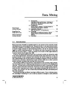
Both Dr. Stephen Bay and one of the anonymous reviewers noted that one implication of the experiments in Section 4.1.1 is that the Euclidean distance works very well for time series! This is true, we did not emphasize this fact in this work, because we already forcefully made this point in [20] (see Section 4.2). Finally, we will show some additional experiments that did not make it to the published paper due to lack of space. The experiment in Figure A is similar to the one shown in Figure 3, but with more classes. 8
10
7
13
9
15
6
14
20
P. Grünwald, A Tutorial Introduction to the Minimum Description Length Principle. To appear as Chapters 1 & 2 of Advances in Minimum Description Length: Theory and Applications. MIT Press, 04.
G.
A. Ortega, B. Beferull-Lozano, N. Srinivasamurthy, and H. Xie. (2000). Compression for Recognition and Content based Retrieval. In Proc. of the European Signal Processing Conference, EUSIPCO'00, Tampere, Finland.
H.
Andrea Baronchelli, Vittorio Loreto (2004). Data Compression approach to Information Extraction and Classification CoRR cond-mat/0403233: (submitted for publication).
I.
C. Noble and D. J. Cook, Graph-Based Anomaly Detection, Proceedings of the Ninth ACM SIGKDD International Conference on Knowledge Discovery and Data Mining, 2003.
J.
Teahan, W.J., Wen, Y., McNab, R.J., Witten, I.H.(2000). A compressionbased algorithm for Chinese word segmentation. Computational Linguistics 26. 375--393
2
16
6
15
9
13
7
12
4
14
20
11
19
2
4
F.
8 5
19
Matt Mahoney (2003). Space Shuttle Engine Valve Anomaly Detection by Data Compression. Unpublished notes. (Thanks to Stan Salvador for bringing this to our attention).
Chunyu Kit. 1998. A goodness measure for phrase learning via compression with the MDL principle. In I. Kruijff-Korbayova(ed.), The ELLSSI-98 Student Session, Chapter 13, pp.175-187. Aug. 17-28, Saarbrueken.
11
18
5
E.
12
17
Matthew B. Kennel (2004). Testing time symmetry in time series using data compression dictionaries. Phys. Rev. E 69, 056208 (9 pages).
J. Segen (1990). Graph Clustering and Model Learning by Data Compression. In Proceedings of the Machine Learning Conference, pages 93-101.
3
10
18 17
3
16 1
1
CDM
Euclidean
Cluster 1 (datasets 1 ~ 5): BIDMC Congestive Heart Failure Database (chfdb): record chf02 Start times at 0, 82, 150, 200, 250, respectively Cluster 2 (datasets 6 ~ 10): BIDMC Congestive Heart Failure Database (chfdb): record chf15 Start times at 0, 82, 150, 200, 250, respectively Cluster 3 (datasets 11 ~ 15): Long Term ST Database (ltstdb): record 20021 Start times at 0, 50, 100, 150, 200, respectively Cluster 4 (datasets 16 ~ 20): MIT-BIH Noise Stress Test Database (nstdb): record 118e6 Start times at 0, 50, 100, 150, 200, respectively
Figure A: Two clusterings on samples from four records from the MITBIH Arrhythmia Database, (Left) Our approach (Right) Euclidean distance
Several people that viewed an early version of the work suggested that the clustering might only work in highly structured data, but not for more “random” data. As a simple sanity check we tried clustering random data and random walk data, as shown in Figure B.
It goes without saying that CDM is by no means perfect, in Figure D, Time Series 3 is incorrectly clustered.
CDM
32 33 35 27 36 30 28 34 31 29 26 25 23 15 17 24 22 16 21 19 18 20 14 13 9 7 11 6 10 2 12 4 8 5 1 3
Euclidean
Figure B: Two clusterings on 15 samples of random walk, and 15 samples of random data
In Figure C, we add some structured data to the mix, to see if CDM is confused by the presence of random data. Video Surveillance: Eamonn, no gun Video Surveillance: Eamonn, gun Video Surveillance: Ann, no gun Video Surveillance: Ann, gun MotorCurrent: healthy 2 MotorCurrent: healthy 1 MotorCurrent: broken bars 2
MIT-BIH Arrhythmia Database www.physionet.org/physiobank/database/qtdb Class 1: Record sel102, Class 2: Record sel104, Class 3: Record sel213
Figure D: The clustering obtained on a 3-class problem. Note that time series 3 (at the bottom of the figure) is not clustered properly
In Figure E we show additional examples from the dataset shown in Figure 8. Although the problems look too simple to be of interest, none of the other four approaches discussed in the paper can find the anomaly in all four examples.
MotorCurrent: broken bars 1 Power Demand: April-June (Italian) Power Demand: Jan-March (Italian)
L-1t
Power Demand: April-June (Dutch) Power Demand: Jan-March (Dutch)
L-1n
random walk random walk random walk random walk random walk random walk
L-1u
random walk random walk
L-1v
random walk random walk rand rand rand rand rand rand rand rand rand rand
Figure C: The clustering obtained on some random walk data, random data, and some highly structured datasets.
00
100 100
200 200
300 300
400 400
500 500
600 600
700 700
800 800
900 900
1000 1000
Figure E: Additional examples from the Aerospace anomaly detection problems, the thickness of the line encodes the level of novelty