Towards Practical and Intelligent Routing in ... - Semantic Scholar

This article has been accepted for publication in a future issue of this journal, but has not been fully edited. Content may change prior to final publication. Citation information: DOI 10.1109/TVT.2015.2481464, IEEE Transactions on Vehicular Technology IEEE TRANSACTIONS ON VEHICULAR TECHNOLOGY, VOL. XX, NO. XX, XXX 2015

1

Towards Practical and Intelligent Routing in Vehicular Ad Hoc Networks Celimuge Wu, Member, IEEE, Yusheng Ji, Member, IEEE, Fuqiang Liu, Member, IEEE, Satoshi Ohzahata, Member, IEEE, and Toshihiko Kato, Member, IEEE

Abstract—Besides the vehicle mobility, the data rate (bitrate) and multi-hop data transmission efficiency (including route length) have significant impact on the performance of a routing protocol for vehicular ad hoc networks (VANETs). Existing routing protocols do not seriously address all these issues, and are not evaluated for a real VANET environment. Therefore, it is difficult for these protocols to attain a high performance and work properly in various scenarios. In this paper, we first discuss the challenges of routing in VANETs based on the data acquired from real-world experiments, and then propose a routing protocol which is able to learn the best transmission parameters by interacting with the environment. The protocol takes into account multiple metrics specifically data transmission rate, vehicle movement and route length. We use both real-world experiments and computer simulations to evaluate the proposed protocol. Index Terms—Vehicular ad hoc networks, routing protocol, rate estimation algorithm, fuzzy logic, Q-Learning.

I. I NTRODUCTION Vehicular ad hoc networks (VANETs) have been attracting interest for their potential roles in intelligent transport systems. Designing an efficient routing protocol is one of the most important issues for VANETs. The performance of a multihop network drops drastically if the end-to-end communication route is not selected properly. The efficiency of a route is dependent on all nodes participating in data transmissions. Lossy wireless channel and vehicle movement make the route selection problem particularly challenging. Most existing routing protocols [1], [3]–[10] take into account vehicle mobility which is one of the most important features of VANETs. However, the transmission rate at the MAC layer is not considered sufficiently. ETX [11] (expected transmission count) is a widely-accepted routing metric for mobile ad hoc networks. The calculation of ETX is based on probe packets. However, the ETX is unable to reflect the system throughput because of the following two reasons: 1) the reception probability of the probe packets is dependent on Copyright (c) 2015 IEEE. Personal use of this material is permitted. However, permission to use this material for any other purposes must be obtained from the IEEE by sending a request to [email protected]. C. Wu, S. Ohzahata and T. Kato are with the Graduate School of Information Systems, University of Electro-Communications, 1-5-1, Chofugaoka, Chofu-shi, Tokyo, 182-8585 Japan (e-mail: {clmg,ohzahata,kato}@is.uec.ac.jp). Y. Ji is with the Information Systems Architecture Research Division, National Institute of Informatics, 2-1-2, Hitotsubashi, Chiyoda-ku, Tokyo 1018430 Japan (e-mail: {kei}@nii.ac.jp). F. Liu is with the School of Electronics and Information Engineering, Tongji University, Shanghai, China (e-mail: [email protected]). Manuscript received 2015.

the size of the probe packets; 2) a small variation in packet reception ratio could not significantly change the expected transmission count but could have a notable effect on the network throughput. Therefore, the transmission rate should be taken into account for the route selection. Many routing protocols utilize position information [3]–[5], [8]–[10] to guide decision making of route selection. However, the use of position information for the link quality estimation has two limitations. First, it is difficult for these protocols to get very accurate position information especially in some road situations, such as tunnels. Second, position information could not reflect the real link quality because the transmission range and path loss exponent could be totally different for different transmission powers and different roads. Opportunistic routing [12] provides an alternative solution by utilizing the broadcast nature of wireless communication and the diversity of packet reception. Due to the lack of the knowledge about receiver, a robust MCS (modulation and coding scheme) is used, resulting in a low throughput. Since the next forwarder node could be different for different frames, frame aggregation (one of the most important techniques supporting high throughput transmissions in 802.11n) is very difficult if not impossible. There have been some multi-path routing protocols [13], [14]. However, finding interferencedisjoint paths is difficult and therefore the throughput improvement is limited. Delay-tolerant networking (DTN) is an approach to provide communication in a situation where continuous network connectivity does not exist. There have been some studies discussing DTN routing protocols for VANETs [15]–[19]. In DTN, data are forwarded using “store and forward” method on the basis of bundles, a series of contiguous data blocks. Therefore, in a connected network which is the scenario we discuss in this paper, DTN protocols cannot provide a short end-to-end delay and efficient end-toend acknowledgment. Several routing protocols [20]–[25] discuss about the use of road-side infrastructure or routing problem around road intersections. However, this paper studies the routing problem from a more general perspective where we do not assume the existence of road-side infrastructure. In VANETs, since the network environment varies for different road types or road segments, the routing protocol needs to be flexible enough to work in various scenarios. This requires the routing protocol to be intelligent enough to tune itself when the environment changes. TCP is the most commonly used transport layer protocol for the Internet. However, TCP throughput of real vehicular ad hoc networks remains underexplored. Many rout-

0018-9545 (c) 2015 IEEE. Personal use is permitted, but republication/redistribution requires IEEE permission. See http://www.ieee.org/publications_standards/publications/rights/index.html for more information.


ing protocols were evaluated based on theoretical analysis and computer simulations. In order to fully understand a protocol’s performance, a real-world implementation and evaluation are required. In this paper, we propose a routing protocol which is able to satisfy all above mentioned requirements. The proposed protocol consists of a rate estimation algorithm and a route selection algorithm. The rate estimation algorithm is able to find the best transmission rate from the hello (probe) packet reception ratio based on a Q-Learning algorithm and a transfer learning algorithm. The route selection algorithm employs a fuzzy logic-based algorithm to evaluate the direct link and uses a Q-Learning algorithm to find the best end-to-end route. We implement the proposed protocol with Ubuntu 12.04 and evaluate the proposed protocol by using a real vehicular ad hoc network. The TCP throughput under different conditions is evaluated and discussed for different road scenarios. We also conduct computer simulations to evaluate the protocol in large scale (in terms of node density) networks. In previous work, we have proposed an idea of using a combination of fuzzy logic and Q-Learning [26] for vehicular sensor networks. However, [26] does not take into account MAC layer transmission rate for the route selection. In this work, we extend the idea of [26] by using reinforcement learning in both the rate estimation algorithm and route selection algorithm. While [26] discussed the routing problem with some unrealistic assumptions (accurate position information and received signal strength information), this paper explains the problem based on experimental results and proposes a practical solution. We also present comprehensive experimental results and simulation results that have not been reported previously. The remainder of the paper is organized as follows. In section II, we give a brief outline of related work and preliminaries. In section III, we describe the problem of the most widely used link quality estimation method. In section IV, we describe the proposed rate estimation algorithm. In section V, we give a detailed description of the proposed route selection mechanism. Experimental results and simulation results are presented in section VI and section VII respectively. In section VIII, we discuss possible improvements. Finally, we present our conclusions in section IX. II. R ELATED WORK

AND

P RELIMINARIES

A. Routing approaches extended from MANET protocols Since a vehicular ad hoc network is a special type of mobile ad hoc networks (MANETs), many studies extend MANET protocols to address the vehicle movement which is one of the most challenging issues for VANET routing protocols. Wang et al. [1] have proposed two protocols (CBRF and CLGF) for small scale VANETs and a two-phase routing protocol (TOPO) for large scale VANETs. Based on AODV [27], CBRF (connection-based restricted forwarding) is able to provide a higher packet delivery ratio by avoiding unnecessary route discovery which is very costly in terms of bandwidth and latency. Toutouh et al. [1] have proposed an approach to tune the parameters of the optimized link state routing (OLSR)

2

protocol for VANETs by using an automatic optimization tool. They have shown that the automatically tuned OLSRs by using metaheuristics are more scalable than the standard version. B. Geographical location based protocols As positioning services like GPS are becoming popular, many protocols utilize location information and road map for the route selection. CLGF (connectionless geographic forwarding) is a location-based approach which forwards a packet by taking account of the MAC layer queue length at the candidate nodes. TOPO incorporates map information in routing. Taleb et al. [3] have proposed a scheme which groups vehicles according to their direction of movement, and chooses the most stable route. Shafiee and Leung [4] have proposed a protocol which prefers a route which has the minimal delay and adequate connectivity. The connectivity is inferred from position information and transmission range. Al-Rabayah and Malaney [5] have proposed a hybrid location-based protocol which combines features of reactive routing with locationbased geographic routing. Yang et al. [6] have proposed an adaptive connectivity aware routing (ACAR) protocol which adaptively selects a route taking into account vehicle densities and traffic light periods. Goonewardene et al. [7] have proposed a clustering scheme which selects optimal cluster heads based on vehicle mobility, locations and direction of travel. Eiza and Ni [8] have used evolving graph theory to model the VANET communication graph on a highway, and proposed a protocol which finds a reliable (based on the mathematical distribution of vehicular movements and velocities) route in the VANET evolving graph. Jiang et al. [9] have utilized a message forwarding metric called coverage capability for the route selection. The metric is calculated based on position information and used to characterize each vehicle’s capability of delivering a message to its target region. Huang and Lin [10] have proposed a forwarding algorithm where each sender node chooses the farthest vehicle as a forwarder node. However, none of above mentioned protocols considers the transmission rate for the route selection. C. Opportunistic routing and multi-path routing Li et al. [12] have proposed LOR, a protocol which can locally realize the optimal opportunistic routing for a largescale wireless network with low control overhead. Due to the nondeterministic feature of packet forwarding, the opportunistic routing cannot utilize the best MCS for the data transmissions. Huang and Fang [13] have explored the efficiency of node-disjoint multi-path routing in VANETs. Li et al. [14] have introduced a geographic multi-path routing protocol, where the alternative paths are as disjoint as possible. Although multipath routing approaches can improve the packet delivery ratio, they also increase the communication overhead if the selected multiple paths are not interference-disjoint, resulting in an increase of MAC layer contention time in the vicinity. D. DTN protocols There have been some DTN protocols for VANETs [15]– [19]. Khabbaz et al. [18] have proposed a protocol which



achieves delay-minimal bundle delivery for two-hop intermittently connected vehicular networks. They developed a mathematical model to evaluate the protocol in addition to computer simulations. Targeting for the same network, Khabbaz et al. [19] have investigated the performance of bundle releasing schemes, and then conducted a mathematical study to evaluate three delay-performance metrics specifically the bundle queueing, transit, and end-to-end delivery delay. Since DTN protocols do not provide end-to-end acknowledgment with packet-level granularity, the applicable scenarios are limited. E. Road-side infrastructure or intersection-based protocols Some protocols have discussed the routing problem with road-side infrastructures and road intersections. Mershad et al. have exploited the infrastructure of roadside units (RSUs) to route packets in VANETs [20]. Shortest-Path-Based TrafficLight-Aware Routing (STAR) has been proposed in [21]. STAR utilizes connected red light segments for packet forwarding. Saleet et al. [22] have proposed an Intersection-based Geographical Routing Protocol (IGRP) for city environments. IGRP efficiently utilizes road intersections to forward a packet. Jerbi et al. [23] have proposed GyTAR, an improved greedy traffic-aware routing protocol which utilizes a dynamic and insequence selection of intersections in the packet forwarding. Nzouonta et al. [24] have proposed a protocol which takes advantage of successions of road intersections to deliver data packets. Chuang and Huang [25] have presented a junctionbased routing protocol which uses control packets to collect the approaching-the-junction information and adapts routing paths according to the information (i.e. practical traffic situations). Since these protocols [20]–[25] are designed for a specific scenario, they are not evaluated in a general scenario. F. Q-Learning and transfer learning Q-Learning [28] is a form of reinforcement learning algorithm that works by estimating the values of state-action pairs without requiring a model of its environment. Q-Learning adjusts behavior through trial-and-error interactions with a dynamic environment. The Q-value Q(s, a) (s ∈ S, a ∈ A) in Q-Learning is an estimate of the value of future rewards if the agent takes a particular action a when in a particular state s. By exploring the environment, the agents build a table of Q-values (Q-Table) to represent evaluation value for each possible action at each environment state. Except when making an exploratory move, the agents select the action with the highest Q-value. In most machine learning methods, a learning task is restarted when training tasks (or data) change. In Q-Learning, an agent has to initialize Q-Table before starting a learning task. In a highly mobile environment, the learning agent (vehicle) could move very fast, which requires the learning algorithm to converge quickly otherwise the learned data cannot reflect the real characteristic of environment. Transfer learning [29] can greatly improve the performance of learning by transferring knowledge between task domains. The core idea of transfer learning is to use the learning experience

3

gained from a task in order to improve learning performance of another related task. In the learning task considered in this paper, the knowledge transfer between vehicles can help a new arriving vehicle to adapt to the network environment faster. G. Fuzzy logic Different from classical set theory, fuzzy set theory [30] uses degrees of membership to express an element. Fuzzy set theory represents incomplete or imprecise information by defining set membership as a possibility distribution. Based on fuzzy set theory, fuzzy logic deals with the concept of approximate rather than precise. For example, we can define a person’s height as being 0.7 “high” and 0.3 “low,” rather than “completely high” or “completely low.” Since fuzzy logic is able to handle very complex reasoning with flexible and tunable fuzzy membership functions and fuzzy rules, it has been widely accepted in industrial communities and used in many real applications. In contrast to numerical values in mathematics, fuzzy logic uses linguistic variables to express the facts. Fuzzy membership functions are used to convert from a numerical value to linguistic variables, and vice versa. Typically, a fuzzy logic-based system consists of three steps: input, process and output steps. The input step converts input numerical values to linguistic variables. The process step calculates the result in a linguistic format based on fuzzy rules (which are defined in the form of IF-THEN statements) and input linguistic variables. The output step is the final step which gets the result in numerical format by converting from the linguistic result. III. P ROBLEM WITH USING HELLO MESSAGE AS AN INDICATOR OF LINK QUALITY IN REAL - WORLD VEHICULAR NETWORKS : EXPERIMENTAL DATA

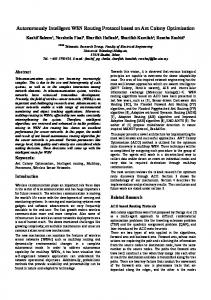
In most routing protocols, hello (probe) packets are used to acquire link status information. However, the hello packet reception ratio is dependent on the size of hello packets and node density. Since hello packets are sent in broadcast, no retransmission is conducted at the MAC layer. As a result, there is a high probability of hello packet loss due to the weak signal strength or collisions with other packets. The hello packet reception ratio is affected by the number of (sending) vehicles, the size of packet and the signal to noise ratio (mainly determined by the distance to the sender). In order to understand the problem, we conducted experiments with real-world vehicular networks where vehicles were communicated with each other using an IEEE 802.11b/g/n wireless radio (2 dBi antenna gain, and 16 dBm transmission power). Figure 1 shows the effect of transmission distance and packet payload size on the probe packet reception ratio. Figure 2 shows the packet reception ratio for different numbers of sender nodes and payload sizes. In addition to transmission distance which directly affects the signal noise ratio at the receiver, the payload size is another important factor which affects the probe packet reception ratio significantly. The number of sender nodes also has a non-negligible effect on the probe packet reception ratio. This means the probe packet reception ratio could be different for different node densities.



0.98

algorithm and considered to be one of the best if not the best. Minstrel defines the measure of successfulness (of packet transmission) as the throughput. Minstrel updates the statistics table for every 100 milliseconds. However, all rates are tried on a regular basis. This is inefficient especially when the rate update interval is small. Although the rate control algorithm can find the best MCS, the throughput is lower than the best fixed rate due to the inefficient rate switching.

0.96 0.94

Packet reception ratio

4

0.92 0.9 0.88 0.86 0.84 0.82

IV. R ATE ESTIMATION ALGORITHM

0.8 Payload size=56B Paiyload size=512B Paiyload size=1024B

0.78 0.76 30

35

40

45

50

55

60

65

70

Distance (m) Fig. 1. Packet reception ratio of broadcast packets for different distances and payload sizes (for the same setting, the packet reception ratio for unicast packets is 100%). 95


90 85 80

A. Rate estimation based on Q-Learning and knowledge transfer Our aim is to find the relationship between the best MCS and the hello (beacon) packet reception ratio. The relationship varies with the change of environment, which requires an online mechanism to deduce the relationship. If the best MCS can be acquired from the probe reception ratio, the sender can set the best transmission rate without trying all possible MCSes. In this way, the throughput can be improved. Since the network environment could be different for different road segments, we use a Q-Learning-based approach to learn the best MCS. In order to improve the convergence speed of the learning, a transfer learning-based approach is used as a supplement.

75

B. Calculation of hello message reception ratio

70 65 60

Payload size=56B Paiyload size=512B Paiyload size=1024B

55 1

2

3

4

5

6

7

8

9

10

Number of sender nodes Fig. 2. Packet reception ratio of broadcast packets for different numbers of sender nodes and payload sizes (broadcast rate: 2 packets per second).

The hello messages are sent with a predefined time interval (1 second by default). In order to get an accurate estimation in dynamic scenarios where frequent topology changes and packet collisions are possible, we use 10 hello intervals as a sliding window size (sampling interval). The hello reception ratio is updated for each hello interval based on the number of received hello messages in the last 10 hello intervals (10 seconds) as HRR(c, x) =

The use of hello message as an indicator of link quality could be dangerous when the packet size is not considered in the evaluation (which is the case of most routing protocols). One may consider using unicast transmissions for probe packets. However, it is difficult to use unicast packet reception ratio to estimate the link quality. This is because the modulation and coding schemes (MCSes) used for unicast packets could be different for different channel conditions. Moreover, there could be retransmissions at the MAC layer which always result in successful delivery of a unicast frame, and therefore the estimation should be conducted by taking into account both the MCS and number of transmissions. Therefore, the use of unicast probe packet for link quality estimation is not practical. Due to the dynamic characteristic of VANETs, it is particularly difficult to define the relationship between the hello packet reception ratio and the link quality (mainly reflected by the transmission rate). Therefore, we require an intelligent algorithm which can adapt to various scenarios. Table I shows the corresponding TCP throughput for different distances and MCSes (modulation and coding scheme) where “AUTO” denotes the default rate control algorithm “minstrel”. Minstrel [31] is a widely implemented rate control

r (c,x)

( CN T

CN Ts (x) , CN Tr (c,x) CN Ts (x) ·

CN Ts (x) >= 10 1 − ( 12 )CN Ts (x) , otherwise,

(1)

where CN Tr (c, x) is the number of hello messages received at c from x, and CN Ts (x) is the number of hello message sent from x. As shown in the equation, we discount those nodes who are only neighbors for less than 10 seconds [in case of CN Ts (x) < 10]. C. Q-Learning Model in the rate estimation algorithm The Q-Learning algorithm that is used in the rate estimation algorithm is defined as follows. The entire network is the environment. Each node (vehicle) in the network is an agent. Each possible hello packet reception ratio (with knowledge about the best MCS) is considered a state of the agent. The set of all possible hello packet reception ratio (we discretize state space within 100 states) in the network is the state space. The learning task is to find the best MCS for the corresponding network environment in relation to the feedback. A node selects the best MCS that it should use for the packet forwarding. Hence the possible set of actions allowed



5

TABLE I TCP THROUGHPUT FOR DIFFERENT DISTANCES AND MCS ES (“0” DENOTES TCP CONNECTION TIMEOUT )

XX XX MCS distance XXX X 30 m 50 m 70 m

MCS 0

MCS 1

MCS 2

MCS 3

MCS 4

MCS 5

MCS 6

MCS 7

AUTO

3.9 3.83 2.26

5.34 4.17 3.17

5.98 5.15 3.81

6.56 8.69 4.72

9.81 2.39 1.06

6.8 0 0

0 0 0

0 0 0

8.97 7.47 4.02

at the node is the set of possible MCSes. A state transition occurs when a MCS is selected. After each MCS selection, the agent gets rewards from the environment, and therefore knows whether the selected MCS is correct or not [change in knowledge about the best MCS (state change)]. Every node maintains a Q-Table which consists of Q-value Q(p, m) whose value ranges from 0 to 1. Here m is a possible MCS, and p is ⌊100×HRR⌋ where HRR is the hello reception ratio calculated 100 as Eq.(1), and ⌊.⌋ is the floor function. Each Q-value represents the evaluation value for choosing a MCS for a hello message reception probability (the hello packet reception ratio is not differentiated between neighbors because what we care is only the relationship between the hello message reception ratio and MCS). D. Exploration and exploitation It is important for a reinforcement learning algorithm to find a balance between exploitation and exploration. In the proposed rate estimation algorithm, exploitation is choosing the best action according to the current knowledge, and exploration is discovering new actions (in order to make the exploitation lead to the global optimum) by selecting a sub-optimal action. We use ǫ-greedy strategy to trade off exploration and exploitation. Based on our experience, ǫ is set to 0.2. E. Exploration: update of Q-values The Q-Table is updated after using auto rate control algorithm. Each node needs to maintain a Q-value for each MCS. Each entry of Q-Table is defined as Q(p, m) where p = 0.01x, p ∈ [0, 1], x ≤ 100 : x ∈ N0 (N0 is the set of all natural numbers including 0, and p is the hello reception ratio). m is the index of MCS specifically a value selected from the set {0,1,2,3,4,5,6,7}. Based on Table I and our observation, we find that the rate control algorithm always can find the best MCS. Therefore, we use the default rate adaptation algorithm (minstrel for Atheros chipset) to guide our learning process. However, we do not use minstrel as it is. This is because minstrel uses 10% of channel time for trying all the possible rates, which is inefficient [32]. Since the proposed routing protocol (we explain the protocol in the next section) can select a relatively stable (in terms of link stability) next hop node, we use minstrel in the exploration phase to find the best rate and use the rate in the exploitation phase (in order to improve the efficiency of transmissions). More specifically, in the exploration phase, we update Q-Table based on the result of the auto rate control algorithm as Q(p, m) ← α × (R + γ × f (m)) + (1 − α) × Q(p, m). (2)

The reward R is   1, R = 0.3,   0,

calculated as if m == MCSauto if m is the second best mode otherwise.

(3)

where MCSauto denotes the best MCS selected by the rate control algorithm. If the MCS indicated by Q-Table is one of the top two MCSes calculated by the rate control algorithm, the corresponding action gets a positive direct reward. Otherwise, the agent gets a discounted reward. In Eq.(2), f (m) is calculated as   if m is one of the top two MCSes 0, f (m) = Q(p, m − 1), if m > MCSauto   Q(p, m + 1), if m < MCSauto . (4) If the selected action (m) is not one of the top two MCSes, the corresponding Q-value is updated based on the neighbor action which is the closest to the MCSauto . When the selected action (m) is larger than MCSauto , the agent gets an indirect reward from the evaluation value of action m − 1 which is closer to the best action (we consider the action taken by minstrel as the best action because minstrel is a widely-accepted algorithm) as compared with the current action. The rationale behind this is that although the current action m is not one of the best two actions but it could be acceptable if its neighbor action m − 1 is good (the Q-value of m − 1 shows the expectation value of the rewards in future steps). This is because an action becomes better when it moves closer to the best action. As shown in Eq.(3), by providing a higher reward to the action which is closer to the top MCS, the algorithm can guide each agent to find the best action for each state. When the selected action is not among the top two best MCSes, the agent does not get direct reward but get a discounted reward which is indicated by f (m). Based on the direct ward (R) and indirect discounted reward f (m), the agent can evaluate an action is whether good or not. Note that α, γ, and the values used for the calculation of reward R are tunable system parameters, and we set these values based on our simulation results. The learning rate α is set to 0.8, and the discount factor γ is set to 0.9 based on our experience (see [33], [34]). In order to give the best action a significantly higher evaluation, we set the reward to 1 and 0.3 for the best action and the second best action respectively. F. Exploitation: set transmission rate based on Q-Table Each sender node uses fixed transmission rate with probability 1 − ǫ (ǫ = 0.2). Here, ǫ is a configurable system



parameter which defines the probability of exploration (see §IV-D). Each sender node uses minstrel for rate selection with probability ǫ (minstrel switches between different rates, which can evaluate all rates). The value of ǫ affects the performance of the proposed rate estimation algorithm. If ǫ is set to 1, the proposed rate estimation algorithm converts to minstrel. Since the rate estimation algorithm can learn the best rate, the proposed protocol can attain a higher throughput by using the best transmission rate to transmit without switching between different rates (MCSes). G. Using transfer learning to improve convergence speed The learned knowledge at a node can be used to reinforce learning at another node, which can improve the learning speed and efficiency. Therefore, the proposed protocol transfers knowledge among agents. In this way, a new agent can learn the new environment faster. The knowledge transfer is conducted as follows: • What to transfer: Transfer learned information (QTable) between agents. • How to transfer: Use broadcast communication to broadcast learned information upon request. • When to transfer: Transfer when a new agent enters the network. When a new vehicle joins the network, the vehicle broadcasts a transfer request message. Upon reception of the message, each node starts a timer of which value is inversely proportional to the inter-vehicle distance (the maximum waiting time is set to 1 second by default; however, this can be tuned according to the network density). Once the timer is expired, a vehicle broadcasts own transmission rate Q-Table if it is itself the first one sending this information. Upon reception of the transferred information, the new vehicle uses the information to update Q-Table in order to speed up the learning process. Here “the network” denotes the set of vehicles that have at least one neighbor. The knowledge transfer happens only when a node changes from not having any neighbor to having neighbors (this can happen when the vehicle turns on or restarts the wireless interface, or the vehicle joins a group of vehicles from an isolated area). There would be no knowledge transfer when two vehicle clusters (group of vehicles) join. V. ROUTE

SELECTION ALGORITHM

A. Algorithm design The efficiency of a multi-hop route depends on all the direct wireless links (one hop links) that constitute the route. The proposed route selection algorithm employs a fuzzy logicbased approach to evaluate a direct wireless link and uses a Q-Learning algorithm to learn the best multi-hop route. A reactive approach based on AODV is used to establish a route to the destination. Figure 3 shows the process for route establishment (without specific explanations, the parameters used for the route discovery process are the same as AODV). When a data transmission is required, the source node broadcasts a route request (RREQ) message. On first receiving the message, each node rebroadcasts it. From the second reception of the

6

same message, each node checks whether the new path (back to the source node) is better than the current one or not (the metric used for evaluating a route will be explained later). We take into account multiple metrics specifically transmission rate (possible transmission rate for the link), vehicle mobility and the number of hops for the “next hop” selection. Upon reception of a RREQ message, the destination node chooses the best next hop (that is, next hop in the direction back to the ˆ ˆ source node) according to its Q-Table (here we use Q-Table to differentiate it from the Q-Table used in the proposed rate estimation algorithm), and uses this next hop node to send a RREP (route reply) packet back to the source node. Upon reception of a RREP message, each subsequent node chooses its next hop node using the same method and forwards the RREP. In this way, the RREP packet is forwarded to the source node. If the RREP is not received in the predefined time interval (the same as AODV) due to route breakage, RREQ will be retransmitted (up to three times) as shown in Fig. 3.

Fig. 3.

Flow chart for route discovery process.

Each node broadcasts hello messages periodically. Upon reception of a hello message, each node estimates the link status of the wireless link (to the hello sender node). The control messages (RREQ, RREP and hello messages) that used in the proposed protocol are extended from AODV, and contain all the field of original AODV messages. In addition, we add some extra information to RREQ and hello messages (the details about the extra information will be explained later in §V-C2 and §V-E). As shown in Fig. 4, the node contacts the rate estimation algorithm (as proposed in §IV) to get the best transmission rate. The node also estimates the relative vehicle movement based on the variation of the hello packet reception ratio. The link status value of the link is calculated based


This article has been accepted for publication in a future issue of this journal, but has not been fully edited. Content may change prior to final publication. Citation information: DOI 10.1109/TVT.2015.2481464, IEEE Transactions on Vehicular Technology IEEE TRANSACTIONS ON VEHICULAR TECHNOLOGY, VOL. XX, NO. XX, XXX 2015 Low

1

Medium High

0.8 Degree

on the corresponding MCS and relative vehicle movement. These metrics are jointly considered using a fuzzy logic. The fuzzy parameters and rules used in the fuzzy logic are easy to modify. Users can tune the fuzzy membership functions and fuzzy rules to make the protocol more suitable for a particular network environment. The fuzzy logic also allows imprecise or contradictory inputs. Q-Learning learns the best transmission parameters (including transmission rate and route) by interacting with environment. Therefore, the proposed protocol can provide a practical and intelligent solution for routing in VANETs.

7

0.6 0.4 0.2 0 0

0.2

0.4

0.6

0.8

1

Hello reception ratio

Fig. 5.

Fuzzy membership function for transmission rate.

of hello packet reception ratio. Link stability factor (we use “link stability” because the factor reflects both vehicle mobility and signal stability) is calculated as ST (c, x) ← (1−α)×STi−1 (c, x)+α×|HRRi (c, x)−HRRi−1 (c, x)| (5) Route selection algorithm and rate estimation algorithm.

B. Using a fuzzy logic-based approach to evaluate each direct link Upon reception of a hello message or an RREQ message from a node x, node c evaluates the link status value ls(c, x) [this will be used in Eq.(6)] by employing a fuzzy logic in terms of data transmission rate and vehicle mobility. 1) Procedure: The following is the procedure for calculating a link status value for a direct link. • Fuzzification: Use predefined linguistic variables and membership functions to convert the transmission rate and vehicle mobility to fuzzy values. • Mapping and combination of IF/THEN rules: Map the fuzzy values to predefined IF/THEN rules and combine the rules to get the rank of the link as a fuzzy value. • Defuzzification: Use a predefined output membership function and defuzzification method to convert the fuzzy output value to a numerical value. 2) Fuzzification: We consider two metrics specifically transmission rate and link stability (including vehicle mobility) in this phase. Regarding transmission rate, MCS 4, MCS 5, MCS 6, and MCS 7 are considered high transmission rates. MCS 3 is considered as medium transmission rate. MCS 0, MCS 1 and MCS 2 are considered as low transmission rate. Based on experimental results shown in Fig. 1, we define the fuzzy membership function for transmission rate as Fig. 5 (take the values for 512 bytes as the default value). The membership function is tuned online based on the result acquired from the proposed rate estimation algorithm. We use the change of hello reception ratio to estimate the vehicle mobility. The rationale behind this is that the change of inter-vehicle distance affects the packet reception ratio of hello packets. When the size of probe packets is the same, the distance is the dominant factor for hello reception ratio. Therefore, we can deduce the vehicle mobility from the change

where HRRi denotes the hello reception ratio at time i. Here, c and x are the current node and neighbor node respectively. The membership function of link stability factor is defined as shown in Fig. 6. Stable Medium 1

Unstable

0.8 Degree

Fig. 4.

0.6 0.4 0.2 0 0

0.2

0.4

0.6

0.8

1

Link stability factor

Fig. 6. Fuzzy membership function for link stability (taking into account vehicle mobility).

TABLE II RULE BASE

Rule1 Rule2 Rule3 Rule4 Rule5 Rule6 Rule7 Rule8 Rule9

Transmission rate High High High Medium Medium Medium Low Low Low

Link stability Stable Medium Unstable Stable Medium Unstable Stable Medium Unstable

Rank Perfect Good Unpreferable Good Acceptable Unpreferable Unpreferable Bad VeryBad

3) Mapping and combination of IF/THEN rules: Based on the fuzzy values of transmission rate and link stability (vehicle mobility) factor, a node uses the IF/THEN rules (as defined in Table II) to calculate the rank of the link between it and the node sending the message (hello message or RREQ message). The linguistic variables of the rank are defined as {Perfect, Good, Acceptable, Unpreferable, Bad, VeryBad}. For example, in Table II, Rule1 may be expressed as follows.



IF Transmission rate is High, and Link stability is Stable THEN Rank is Perfect. Since there can be multiple rules applying at the same time, we use the Min-Max method to combine their evaluation results. In the Min-Max method, for each rule, the minimal value of the antecedent is used as the final degree. When combining different rules, the maximal value of the consequents is used. 4) Defuzzification: The output membership function is defined as in Fig. 7. Here we use the Center of Gravity (COG) method to defuzzify the fuzzy result. The x coordinate of the centroid is the defuzzified value, which shows the evaluation value of the direct link to the message sender node. 1

VeryBad

Bad

Unpreferable

Acceptable

Good

Perfect

0.8 0.6 0.4 0.2 0 0

Fig. 7.

0.2

0.4

0.6

0.8

1

Output membership function.

C. Q-Learning-based multi-hop route evaluation 1) Q-Learning model of the route selection algorithm: The Q-Learning algorithm that is used in the route selection is defined as follows. The entire vehicular ad hoc network is the environment. Each packet P (s, d), indexed by its source node s and destination node d is an agent. Each node in the network is considered a state of the agent. The set of all nodes in the network is the state space. A node selects the next hop that it should forward a packet to. Hence the possible set of actions allowed at the node is the set of one-hop neighbors. A state transition occurs when a packet is delivered from one node to ˆ its neighbor. Every node maintains a Q-Table which consists ˆ ˆ of Q-value Q(d, x) whose value ranges from 0 to 1, where d is the reference node and x is the next hop to the reference node. ˆ 2) Update of Q-values: Each node maintains an evaluation value [ls(s, x) in Eq.(6)] for each one-hop neighbor. The evaluation value is calculated using the fuzzy logic described in §V-B. These evaluation values are used for updating the ˆ Q-Table. ˆ The Q-Table is updated upon the reception of hello messages or RREQ messages. Each node needs to maintain a ˆ Q-value for each one-hop neighbor, the traffic source node ˆ and destination node. Each node broadcasts the Q-values using hello messages. RREQ messages are used to establish ˆ a route to the destination. Each node attaches its Q-value for the source node before broadcasting a RREQ message. By ˆ attaching the Q-value (to the traffic source node) to a RREQ message, the recent topology information can be delivered to the destination node.

8

ˆ Each Q-value is initialized to 0. Upon reception of a message (hello message or RREQ message) from node x, node ˆ c updates the corresponding Q-value to the node d as n o ˆ c (d, x) ← α × ls(c, x) × R ˆ + γ × maxy∈Nx Q ˆ x (d, y) Q ˆ c (d, x). + (1 − α) × Q

(6)

Here, ls(c, x) is the evaluation value of the link between node c and x (which is calculated as explained in §V-B). The learning rate (α) and the discount factor (γ) are the same as ˆ Eq.(2). We call maxy∈Nx Qx (d, y) the maximal Q-value of x ˆ to node d. The reward R is calculated as ( 1, if c ∈ Nd ˆ R= (7) 0, otherwise where Nd denotes the neighbor set of node d (we use “neighbor” to denote one-hop neighbor throughout the paper). When node c is a neighbor of the node d, the reward is 1 ˆ and otherwise 0. Note that there is only one Q-value for each pair of state and action. For each exploration action (upon ˆ reception of hello message), the corresponding Q-value is updated as shown in Eq.(6). Since the hello messages are sent periodically, the knowledge about the network is updated periodically. As shown in Eq.(6), the reward is discounted with an increase of the number of hops (larger number of hops ˆ results in smaller reward and smaller Q-value). The reward is also discounted depending on the link status values of the ˆ links traversed. As a result, a Q-value represents the quality of a next hop from a multi-hop perspective. This ensures that the proposed protocol can find the best route in terms of multi-hop performance. Upon the first reception of a RREQ message, each interˆ mediate node attaches its maximal Q-value for the source node to the RREQ message, and rebroadcasts the RREQ. As shown in Fig. 8, upon reception of a RREQ message from ˆ S) according to the source node S, node R1 calculates Q(S, Eq.(6), and attaches the result to RREQ message [since R is 1 ˆ S) will be 0.72]. R2 does the same and ls(R1, S) is 0.9, Q(S, calculation after receiving the RREQ from R1. Upon reception ˆ of a RREQ message, the destination node (D) updates its QTable and sends back a RREP message to the sender node. The neighbor node (neighbor node of the destination node) ˆ which has the maximal Q-value is selected as the next hop node (R2 is selected for Fig. 8); since we are considering a reply message, “next hop” here means the next hop in the direction back to the source node, that is the node that will form the “previous node” for the eventual data transmission. After reception of a RREP packet, each node chooses the next hop using the same method until the source node is reached. The path traversed by the RREP packet will be the route for data delivery. Since each forwarder node selects its next hop node, the best possible route can be found (in Fig. 8, the route “S → R1 → R2 → D” will be selected). D. Exploitation and exploration In the proposed route selection algorithm, exploitation and exploration do not contradict each other. The algorithm uses



Fig. 8.

9

RREQ message, Q-Table update and RREP message.

the next hop node that has maximal Q-value to forward a data packet (exploitation). Every node updates their Q-values upon reception of hello messages and route request messages from its neighbors (exploration). Hello messages are exchanged periodically, so every node is aware of which neighbor has become the best. Each node also updates its knowledge (Qvalues) upon reception of a route request message. Since a route is determined after the update of the Q-values, the action selected is always the best. E. Route switching We use a dynamic route switching mechanism to change a route if a better one is detected. Each sender node (including the source node and forwarder nodes) changes route according ˆ to Q-Table without using RREQ messages. As mentioned ˆ before, the Q-Table update is conducted upon reception of hello messages or RREQ messages. In the route maintenance ˆ phase, the Q-Table is updated only by hello messages. Each ˆ node attaches the maximal Q-values for the active destination nodes to the hello messages. Upon reception of a hello ˆ message, each node updates its Q-Table, and checks whether a new better route is available or not (see Fig. 9). The details ˆ about the Q-Table update are shown in Fig. 10. As shown in Fig. 10, upon reception of hello message from node D, node R2 updates its knowledge about the destination node (D), ˆ and sends the maximal Q-value to D with hello messages. Once this information is reached the source node S, the node checks whether the corresponding path (“S → R2 → D”) is better than the current route (‘S → R4 → D”) or not. Since the new path is better, node S starts to use the new route (“S → R2 → D”) for data transmissions. The time required for transmitting link status information is dependent on the hello interval and the number of hops. Therefore, we only switch route when the number of hops to the destination is equal to or smaller than Hs . The value of Hs can be set based on the hello interval. In this paper, we set Hs to 2 because for hello interval of 1 second, a larger value could possibly result in inefficient route change according to our simulation results. Each neighbor of the destination (of a traffic flow) ˆ node broadcasts the corresponding Q-value by attaching it to hello messages. By using the hello messages, each node can ˆ update its Q-values for the destination node which is located within Hs hops. VI. E XPERIMENTAL R ESULTS We used a real-world vehicular ad hoc network to evaluate the performance of the proposed protocol. The proposed

Fig. 9.

Fig. 10.

Flow chart for hello processing.

Hello message, Q-Table update, and route switching.

protocol was implemented in Ubuntu 12.04 LTS. We used 10 cars to generate the VANETs where each car was equipped with 1 laptop computer (a wireless interface attached to it) (see Fig. 11). The cars (laptops) ran in ad-hoc mode and communicated with each other using 2.4GHz IEEE 802.11b/g/n wireless radio (2 dBi antenna gain, 16 dBm transmission power). We evaluated the protocol in 3 different scenarios: (1) a oneway straight road, (2) a two-way road straight road, and (3) a street scenario with intersections (see Fig. 12). In the one-way scenario, all cars traveled in the same direction (the maximum allowable velocity was 70 km/h; road length was 5 km). In the two-way scenario, 10 cars were divided into 2 groups (each with 5 cars) and driven in two different directions. This scenario is to evaluate the route selection efficiency in terms of vehicle mobility. In the street scenarios, there was an intersection for each 300 m. The length of the red/green signal was 40 seconds. For each case, we used the average value of ten measurements (10 runs, each with 5 minutes). In order to clearly understand the protocol performance, we generated only one TCP flow for each run. The proposed protocol was compared



Fig. 12.

10

Movement pattern: (left) straight road scenario (right) street scenario.

TCP throughput (Mbps)

12

10

8

6

4

2 AODV-ETX (broadcast probe) Proposed HLAR 0 30

Fig. 11.

Experimental environment.

35

40

45

50

55

60

65

70

Distance (m) Fig. 13. TCP throughput for various inter-vehicle distances (1-hop scenario).

with AODV-ETX (AODV with ETX [11]), and HLAR [5]. AODV-ETX selects routes by taking account of the expected transmission count which is calculated based on the reception probability of probe packets. In the following results, “AODVETX (broadcast probe)” shows the result when the broadcast probe packets are used. “AODV-ETX (unicast probe)” shows the results when unicast probe packets are used. HLAR is a hybrid routing protocol for VANETs which combines AODVETX with greedy-forwarding geographic routing. The error bars indicate the 95% confidence intervals. A. TCP throughput for various inter-vehicle distances Figure 13 shows one-hop TCP throughput (the number of hops from the source node to the destination node is 1) for various inter-vehicle distances. We show the one-hop TCP throughput comparison in order to show the advantage of the proposed rate estimation algorithm clearly (comparison for multi-hop TCP throughput will be shown later). The difference between the proposed protocol and other protocols shows that the advantage of the proposed rate estimation algorithm is notable. The proposed protocol is able to learn the best transmission rate in the exploration phase. In the exploitation phase,

the proposed protocol uses the best rate without transmitting packets on all rates, which can improve the total throughput. As shown in Fig. 13, by using the proposed rate estimation algorithm, we can achieve notable performance improvement even for one-hop transmissions. B. TCP throughput for various initial source-destination distances in straight road scenario Figure 14 shows the TCP throughput for various initial source-destination distances. The TCP connection was established between two vehicles moving in the same direction. The initial source-destination distance shows the distance of the source node and destination node at the time the TCP flow was established. We use the initial source-destination distance as a reference because it determines the number of hops from the source node to the destination node at the beginning of data transmission (note that the number of hops could be different for different protocols, which is the reason we use the initial distance as a reference). The proposed protocol attains the best performance. This is because the protocol takes into account the transmission rate and vehicle movement for the route



plains the TCP throughput difference of the proposed protocol and other protocols (see Fig. 14). The proposed protocol can attain high UDP packet delivery ratio even when the source-destination distance is large. By selecting better endto-end routes, the proposed protocol reduces the number of retransmissions at the TCP layer, which can improve the TCP performance significantly.

AODV-ETX (broadcast probe) (one-way) AODV-ETX (unicast probe) (one-way) Proposed (one-way) AODV-ETX (broadcast probe) (two-way) AODV-ETX (unicast probe) (two-way) Proposed (two-way) HLAR (one-way) HLAR (two-way)

8

6

C. TCP throughput for various initial source-destination distances in street scenario

4

2

0 40

60

80

100

120

140

Distance (m) Fig. 14. TCP throughput for various initial source-destination distances (oneway road and two-way road).

selection. When the inter-vehicle distance is 60 m, “AODVETX (broadcast probe)” and “AODV-ETX (unicast probe)” intend to select 1-hop route. However, since the signal quality is poor, a low transmission rate (MCS 2) is used. Having no consideration for the transmission rate, HLAR shows a similar performance with “AODV-ETX (broadcast probe)”. The main advantage of HLAR over “AODV-ETX (broadcast probe)” is the utilization of position information for the route discovery, which has very limited effect on the performance in a low-density network. When the source-destination distance (the number of hops) increases, the link quality estimation of “AODV-ETX (unicast probe)” performs worse because unicast probe packets can be delivered with a very high probability due to multiple retransmissions at the MAC layer. Since “AODVETX (broadcast probe)” and “AODV-ETX (unicast probe)” do not consider vehicle mobility, they show a lower performance in the two-way scenario than one-way scenario.

Figure 16 shows TCP throughput for various initial sourcedestination distances in street scenario [the vehicle movement follows Fig. 12 (right)]. At an intersection, the sourcedestination distance changes due to the change of inter-vehicle distance. We observe that the proposed protocol can attain much better performance in this scenario as compared with the straight road scenarios. This is because when vehicles are stopping at an intersection, the proposed protocol can change to a shorter route and therefore improve the throughput. For AODV-ETX and HLAR, an existing route does not change until it is broken. This proves that the dynamic route switching mechanism is particularly important for intersection scenarios. 12



12

10

11

AODV-ETX (broadcast probe) AODV-ETX (unicast probe) Proposed HLAR

10

8

6

4

2

0 40

UDP packet delivery ratio

60

80

100

120

140

Distance (m)

1

Fig. 16. TCP throughput for various initial source-destination distances (the distance is shorter when the vehicles stop at the intersections) in street scenario.

0.8

0.6

D. Number of hops 0.4

0.2


0 40

60

80

100

120

140

Distance (m) Fig. 15. UDP packet delivery ratio for various initial source-destination distances (two-way road).

UDP packet delivery ratio for various initial sourcedestination distances is shown in Fig. 15. This figure ex-

Figure 17 shows the average number of hops for straight road scenario (one-way). The proposed protocol intends to use longer routes as compared with other protocols due to the consideration of MCS used in data transmissions. “AODVETX (unicast probe)” shows the shortest number of hops because the unicast probe packets result in overestimation of the link status. Figure 18 shows the average number of hops for street scenario. In street scenario, the proposed protocol shows lower number of hops as compared with straight road scenario due to the route changes at intersections. When the vehicle density increases, the time percentage stopping at the intersections becomes lower, resulting in increase of route length.



4.5

12 AODV-ETX (broadcast probe) AODV-ETX (unicast probe) Proposed HLAR

Number of route updates

4 3.5

Number of hops

12

3 2.5 2 1.5 1

10


8

6

4

2

0.5 0

0 40

60

80

100

120

140

40

Distance (m)

60

80

100

120

140

Distance (m)

Fig. 17. Number of hops for various initial source-destination distances (one-way road).

Fig. 20. Average number of route updates for various initial sourcedestination distances in street scenario.

4 3.5


Figure 19 shows the average number of route updates for straight road scenario (two-way). The route updates of AODVETX and HLAR are due to route breakage and the corresponding route re-establishment. Since the proposed protocol can choose the best route, the route breakage does not happen in this scenario. For street scenario (see Fig. 20), the proposed protocol updates route because a better route is available when vehicles stopping at an intersection.

Number of hops

3 2.5 2 1.5 1

VII. S IMULATION RESULTS

FOR LARGE - SCALE

VEHICULAR NETWORKS

0.5

TABLE III S IMULATION E NVIRONMENT

0 40

60

80

100

120

140

Distance (m) Fig. 18. Number of hops for various initial source-destination distances in street scenario.

E. Number of route updates


0.6

0.5


0.4

0.3

0.2

0.1

0 40

60

80

100

120

140

Distance (m) Fig. 19. Average number of route updates for various initial sourcedestination distances (two-way road).

Topology Mobility Packet payload MAC Packet loss Simulation time

Straight road 2000m, 4lanes

Intersection Scenario 1500m × 1500m, 5 × 5 street, 4 lanes Ref. [36] 1024 bytes IEEE 802.11p MAC Based on experimental data 10 minutes

We used ns-2.34 [35] to conduct simulations in straight road scenarios, and street scenarios with intersections by using [36] as the mobility generator (see Table III). The mobility pattern generated by [36] is able to simulate realistic vehicle movements by addressing spatial dependence and high temporal dependence, and imposing strict geographic restrictions on the vehicle movement. The configuration is easy, and users only need to specify road topology, the maximum allowable velocity, and the number of vehicles (overtaking scenarios are generated by defining road and vehicle velocity properly). The maximum allowable vehicle velocity was 70 km/h. Wireless channel parameters were set based on Fig. 1 and Table I. In terms of the packet reception probability for each distance, basic reference points specifically the probabilities for {30m, 50m, 70m} were set based on our measurement results and others were set proportionally according to the distance from the reference points. In the street scenarios, the distance between two intersections was 300 m. There was



always one traffic (randomly selected) flow transmitting 5 Mbytes files from the source to the destination. After the end of each transmission, the source node and destination node were reselected. The maximum distance between the source node and destination node was set to 150 m considering the transmission range (see Fig. 1). The length of the red/green signal was 40 seconds.

13

algorithm. The consideration of end-to-end throughput in the route selection also contributes to the result. AODV-ETX chooses shorter routes (longer inter-vehicle distance) which are unable to provide a high end-to-end throughput. The result for street scenarios is shown in Fig. 22. The proposed protocol shows a significant advantage over other protocols. From these simulation results, we can know that the proposed protocol is scalable in terms of node density.

A. TCP throughput B. Number of hops 6

5 3 4

Number of hops


3.5

3

2

1


2.5

2

1.5


0.5

0 0

50

100

150

200

250

300

350

400 0

Number of vehicles per km

0

Fig. 21. TCP throughput for various numbers of nodes per km road (straight road scenarios).

50

100

150

200

250

300

350

400

Number of vehicles per km Fig. 23. Number of hops for various numbers of nodes per km road (straight road scenario).

7 2.5

2

5

Number of hops


6

4

3


1

1.5

1

0.5 AODV-ETX (broadcast probe) AODV-ETX (unicast probe) Proposed HLAR

0 0

50

100

150

200

250

300

350

400

Number of vehicles per km Fig. 22. TCP throughput for various numbers of nodes per km road (street scenarios).

Figure 21 shows the TCP throughput for various numbers of vehicles per km. When the number of vehicles is 50, the network is sparsely connected. This is why all protocols show a lower throughput. As the node density increases, the frame collision ratio increases (due to increase of hello packets), which is a main factor resulting in the performance degradation of AODV-ETX. HLAR shows better performance by using position information to guide the route request phase of AODV-ETX. The proposed protocol can attain much better TCP throughput by using the proposed rate estimation

0 0

50

100

150

200

250

300

350

400

Number of vehicles per km Fig. 24. Number of hops for various numbers of nodes per km road (street scenario).

Figure 23 and Fig. 24 show the average number of hops for straight road scenario and street scenario respectively. For the proposed protocol, the average route length increases with the node density due to the decreasing effect of route change mechanism. When stopping at a road intersection, a route change occurs and a shorter route will be selected, resulting in a smaller number of hops. However, when the vehicle density increases, the average route length increases slightly because the time percentage stopping at an intersection becomes lower.



Size of generated control packets (KB)

C. Number of route updates 80


70 60 50 40 30 20 AODV-ETX (broadcast probe) AODV-ETX (unicast probe) Proposed HLAR

10

14


50

40

30

20

10

0 0

50

100

150

200

250

300

350

400


0 50

100

150

200

250

300

350

400

Number of vehicles per km Fig. 25. Number of route updates for various numbers of nodes per km road (straight road scenario).

100

80

60

40


50

40

30

20

10

0 0

20


0 0

50

100

150

50

100

150

200

250

300

350

400

Number of vehicles per km 200

250

300

350

400

Number of vehicles per km Fig. 26. Number of route updates for various numbers of nodes per km road (street scenario).

Figure 25 and Fig. 26 show the average number of route updates (including both route creation for a new flow, and route change) for straight road scenario and street scenario respectively. The proposed protocol shows higher number of route updates than “AODV-ETX (broadcast probe)” and HLAR due to the preemptive route change mechanism. D. Control overhead Figure 27 and Fig. 28 show the size of generated control packets (including MAC layer retransmissions) per second for straight road scenario and street scenario respectively. In the proposed protocol, each node attaches position information and a small part of Q-Table to hello messages. However, this does not incur too much impact on the control overhead. The main control overhead comes from the hello message exchange (the hello message overhead increases proportionally with the node density) which is considered to be important for many applications.

Fig. 28. Size of generated control packets per second for various numbers of nodes per km road (street scenario).

E. End-to-end delay 0.2 AODV-ETX (broadcast probe) AODV-ETX (unicast probe) Proposed HLAR

0.18 0.16

End-to-end delay (s)


120

Fig. 27. Size of generated control packets per second for various numbers of nodes per km road (straight road scenario).

Size of generated control packets (KB)

0

0.14 0.12 0.1 0.08 0.06 0.04 0.02 0 0

50

100

150

200

250

300

350

400

Number of vehicles per km Fig. 29. End-to-end delay for various numbers of nodes per km road (straight road scenario).



15

VIII. D ISCUSSIONS

0.25 AODV-ETX (broadcast probe) AODV-ETX (unicast probe) Proposed HLAR

End-to-end delay (s)

0.2

0.15

0.1

0.05

0 0

50

100

150

200

250

300

350

400


We conducted real-world experiments to evaluate the performance of the proposed protocol. We found that it is possible to achieve around 2 Mbps TCP throughput for 150 m distance (average transmission range was around 40 m as shown in Fig. 1), which is sufficient for most applications. The performance also can be improved by increasing the transmission power. As a reference, we also launched experiments where each wireless transceiver has 5dBi antenna gain and 20 dBm transmission power. Figure 32 and Fig. 33 show the UDP packet delivery ratio and TCP throughput for different distances respectively (1-hop transmission). From these experimental results, we can know that the coverage area can be improved significantly by increasing the transmission power.

Fig. 30. End-to-end delay for various numbers of nodes per km road (street scenario).

0.95


Figure 29 and Fig. 30 show the average end-to-end delay for straight road scenario and street scenario respectively. The proposed protocol shows the lowest delay due to the following reasons. First, the protocol can reduce the propagation time of each packet, and number of retransmissions at the MAC layer by using a better MCS. Second, the proposed protocol takes into account multi-hop efficiency in the route selection. For the street scenario, the route change mechanism also contributes to the short delay.

1

0.9

0.85

0.8

Packet reception ratio 0.75

F. Convergence of the proposed Q-learning algorithm

70

80

90

100

110

120

130

140

Distance (m) Fig. 32. Packet reception ratio of unicast packets for different distances (5 dBi antenna gain, and 20 dBm transmission power). 1

9

0.8

0.6

0.4

0.2 1-hop 2-hop 3-hop 0 1

2

3

4

5

6

7

8

9

10


Value

8 7 6 5 4 3 2

Time (s) 1

ˆ Fig. 31. Q-value for a new link status information (“n-hop” shows the ˆ variation in Q-value at a n-hop distance).

TCP throughput 0 70

80

90

100

110

120

130

140

Distance (m) ˆ Figure 31 shows the variation in Q-value with time. “1ˆ hop”, “2-hop” and “3-hop” show the variation in Q-value at 1-hop, 2-hop, and 3-hop distance respectively. When the number of hops is 3, the protocol converges in 6 seconds. ˆ Here, the hello interval is 1 second, and the Q-value is updated for each hello interval. When the hello interval is shorter, the convergence speed is faster.

Fig. 33. TCP throughput for different distances (5 dBi antenna gain, and 20 dBm transmission power).

Rate control algorithm is another factor that directly affects the performance of a multi-hop transmission. Current rate control algorithm is not discussed and designed for ad hoc networks. Since the transmission rate is a dominant factor of



the end-to-end performance, an efficient rate adaptation considering multiple destinations should be discussed seriously. In the proposed protocol, all parameters are set based on our experience [33], [34]. The users can tune these parameters based on their requirements. The most important parameter, the transmission rate membership function, is tuned via a Q-Learning algorithm. For the proposed rate selection algorithm, ǫ defines the probability of exploration. By setting an appropriate value for ǫ, we can manage the tradeoff between efficiency and accuracy. For both the rate estimation algorithm and route selection algorithm, the learning rate and discount factor have a notable impact on the performance. The learning rate parameter limits the speed of learning, which governs how quickly the Q-values can change with each state/action change. The discount factor controls the value placed on future rewards. If the value is low, immediate rewards are optimized, while higher values of the discount factor make the learning algorithm to count future rewards more strongly. Since it is difficult if not impossible to use mathematical model to explain the optimal values for these parameters, the users have to tune these parameters according to their requirements. We use a reinforcement learning approach to find the best route instead of using optimal route selection based on theory. This is because the accurate knowledge about the whole network topology is impossible due to the communication overhead. The computation overhead of the proposed protocol is negligible because each node only needs to maintain own Qˆ Table (route selection algorithm) and Q-Table (rate estimation algorithm), and the vehicles could have enough computational capability. Note that it is difficult to accurately estimate the link status in real-world scenarios because the channel condition frequently changes with vehicle movement. The proposed protocol is robust to estimation errors because the reinforcement learning can smooth out most errors by taking into account the previous value for the update of Q-value. Moreover, since it is more important to consider the relative link status value than the absolute value (we only care which one is better), the proposed protocol is able to find the best route efficiently. Based on fuzzy logic and reinforcement learning, the proposed protocol can provide an intelligent and flexible solution for routing in VANETs.

IX. C ONCLUSIONS We examined the problem of existing routing protocols in real-world vehicular ad hoc networks, and then proposed an intelligent multi-hop routing protocol which selects routes by taking into account the transmission rate, vehicle mobility and number of hops. The protocol employs a Q-Learning-based approach to estimate transmission rate from the hello packet reception ratio. For the route selection, the protocol uses a fuzzy logic-based algorithm to evaluate the direct link and uses a Q-Learning algorithm to learn the best end-to-end route. We used real-world experiments and computer simulations to show the advantage of the proposed protocol over existing alternatives.

16

ACKNOWLEDGMENT This work was supported by JSPS KAKENHI Grant Number 25730053, and the National Natural Science Foundation of China (Key Program) under Grant 61331009. R EFERENCES [1] W. Wang, F. Xie and M. Chatterjee, “Small-Scale and Large-Scale Routing in Vehicular Ad Hoc Networks,” IEEE Trans. Veh. Technol., vol.58, no.9, pp.5200–5213, 2009. [2] J. Toutouh, J. Garcia-Nieto, and E. Alba, “Intelligent OLSR Routing Protocol Optimization for VANETs,” IEEE Trans. Veh. Technol., vol.61, no.4, pp.1884–1894, 2012. [3] T. Taleb, E. Sakhaee, A. Jamalipour, K. Hashimoto, N. Kato, and Y. Nemoto, “A Stable Routing Protocol to Support ITS Services in VANET Networks,” IEEE Trans. Veh. Technol., vol.56, no.6, pp.3337–3347, 2007. [4] K. Shafiee and V. C.M. Leung, “Connectivity-aware minimum-delay geographic routing with vehicle tracking in VANETs,” Ad Hoc Netw., vol.9, pp.131–141, 2011. [5] M. Al-Rabayah and R. Malaney, “A New Scalable Hybrid Routing Protocol for VANETs,” IEEE Trans. Veh. Technol., vol.61, no.6, pp.2625– 2635, 2012. [6] Q. Yang, A. Lim, S. Li, J. Fang and P. Agrawal, “ACAR: Adaptive Connectivity Aware Routing for Vehicular Ad Hoc Networks in City Scenarios,” Mobile Netw. Appl., vol.15, pp.36–60, 2010. [7] R.T. Goonewardene, F.H. Ali and E. Stipidis, “Robust mobility adaptive clustering scheme with support for geographic routing for vehicular ad hoc networks,” IET Intell. Transp. Syst., vol.3, no.2, pp.148–158, 2009. [8] M. H. Eiza and Q. Ni, “An Evolving Graph-Based Reliable Routing Scheme for VANETs,” IEEE Trans. Veh. Technol., vol.62, no.4, pp.1493– 1504, 2013. [9] R. Jiang, Y. Zhu, T. He, Y. Liu, and L.M. Ni, “Exploiting TrajectoryBased Coverage for Geocast in Vehicular Networks,” IEEE Trans. Parallel and Distrib. Syst., vol.25, no.12, pp.3177–3189, 2014. [10] C.-M. Huang and S.-Y. Lin, “Timer-based greedy forwarding algorithm in vehicular ad hoc networks,” IET Intelligent Transport Systems, vol.8, no.4, pp.333–344, 2014. [11] D.S.J. De Couto, D. Aguayo, J. Bicket and R. Morris, “A HighThroughput Path Metric for Multi-Hop Wireless Routing,” in Proc. ACM MOBICOM, pp.134–146, 2003. [12] Y. Li, A. Mohaisen, and Z.-L. Zhang, “Trading Optimality for Scalability in Large-Scale Opportunistic Routing,” IEEE Trans. Veh. Technol., vol.62, no.5, pp.2253–2263, 2013. [13] X. Huang and Y. Fang, “Performance Study of Node-Disjoint Multipath Routing in Vehicular Ad Hoc Networks,” IEEE Trans. Veh. Technol., vol.58, no.4, pp.1942–1950, 2009. [14] P. Sermpezis, G. Koltsidas, and F.-N. Pavlidou, “Investigating a JunctionBased Multipath Source Routing Algorithm for VANETs,” IEEE Commnu. Letters, vol.17, no.3, pp.600–603, 2013. [15] N. Benamar, M. Benamar, and J.M. Bonnin, “Routing protocols for DTN in vehicular environment,” in Proc. ICMCS, pp.589–593, 2012. [16] K.C. Lee and M. Gerla, , “Opportunistic vehicular routing,” in Proc. European Wireless Conference, pp.873–880, 2010. [17] S.M. Tornell, C.T. Calafate, J.-C. Cano, and P. Manzoni, , “DTN Protocols for Vehicular Networks: An Application Oriented Overview,” in IEEE Commun. Surveys Tuts., vol.17, no.2, pp.868–887, 2015. [18] M. J. Khabbaz, H. M. K. Alazemi, and C. M. Assi, “Delay-Aware Data Delivery in Vehicular Intermittently Connected Networks,” IEEE Trans. Commun., vol.61, no.3, pp.1134–1143, 2013. [19] M. J. Khabbaz, W. F. Fawaz, and C. M. Assi, “Modeling and Delay Analysis of Intermittently Connected Roadside Communication Networks,” IEEE Trans. Veh. Technol., vol.61, no.6, pp.2698–2706, 2012. [20] K. Mershad, H. Artail and M. Gerla, “We Can Deliver Messages to Far Vehicles,” IEEE Trans. Intelligent Transportation Systems, vol.13, no.3, pp.1099–1115, 2012. [21] J.-J. Chang, Y.-H. Li, W. Liao, I.-C. Chang, “Intersection-based routing for urban vehicular communications with traffic-light considerations,” IEEE Wireless Commun., vol.19, no.1, pp.82–88, 2012. [22] H. Saleet, R. Langar, K. Naik, R. Boutaba, A. Nayak, and N. Goel, “Intersection-Based Geographical Routing Protocol for VANETs: A Proposal and Analysis,” IEEE Trans. Veh. Technol., vol.60, no.9, pp.4560– 4574, 2011.



[23] M. Jerbi, S.-M.Senouci, T. Rasheed and Y. Ghamri-Doudane, “Towards Efficient Geographic Routing in Urban Vehicular Networks,” IEEE Trans. Veh. Technol., vol.58, no.9, pp.5048–5059, 2009. [24] J. Nzouonta, N. Rajgure, G. Wang and C. Borcea, “VANET Routing on City Roads Using Real-Time Vehicular Traffic Information,” IEEE Trans. Veh. Technol., vol.58, no.7, pp.3609–3626, 2009. [25] P.-J. Chuang and T.-L. Huang, “Efficient vehicular ad-hoc networks routing based on junctions,” IET Communications, vol.9, no.4, pp.487– 493, 2015. [26] C. Wu, S. Ohzahata and T. Kato, “Learning route from beaconing and interest dissemination in vehicular sensor networks,” in Proc. TSSA, pp.49–54, 2011. [27] C. Perkins, and E. Belding-Royer, Ad hoc On-Demand Distance Vector (AODV) Routing, RFC 3561, Jul. 2003. [28] C. Watkins, Learning from Delayed Rewards, PhD thesis, King’s College, Cambridge, 1989. [29] S. J. Pan, and Q. Yang , “ A Survey on Transfer Learning ,” IEEE Trans. Knowledge and Data Engineering, Vol.22, No.10, pp.1345–1359, 2010. [30] George J. Klir, Ute St. Clair, and Y. Bo, Fuzzy set theory: foundations and applications, Prentice-Hall, Inc. [31] Minstrel - Linux Wireless, http://madwifi-project.org/svn/madwifi/trunk/ath rate/minstrel/, Accessed on June. 1, 2014. [32] D. Xia, J. Hart, and Q. Fu, “Evaluation of the Minstrel rate adaptation algorithm in IEEE 802.11g WLANs,” in Proc. IEEE ICC, pp.2223–2228, 2013. [33] C. Wu, K. Kumekawa and T. Kato, “Distributed Reinforcement Learning Approach for Vehicular Ad Hoc Networks,” IEICE Trans. Commun., vol.E93-B, no.6, pp.1431–1442, 2010. [34] C. Wu, K. Kumekawa and T. Kato, “A Dynamic Route Change Mechanism for Mobile Ad Hoc Networks,” International Journal of Communication Networks and Distributed Systems, vol.7, no.1/2, pp.4– 17, 2011. [35] The Network Simulator - ns-2, http://www.isi.edu/nsnam/ns/, Accessed on Dec. 23, 2012. [36] F. Bai, N. Sadagopan, and A. Helmy, “Important: A Framework to Systematically Analyze The Impact of Mobility on Performance of Routing Protocols for Adhoc Networks,” Proc. IEEE INFOCOM, pp.825–835, 2003.

17

Fuqiang Liu is a Professor in the School of Electronics and Information Engineering, Tongji University, Shanghai, China. He received his Bachelor degree from Tianjin University in 1987, and Ph.D degree from China University of Mining and Technology in 1996. Currently, he serves as the Director of the Broadband Wireless Communication and Multimedia Laboratory at Tongji University. He is a Guest Professor of the National Institute of Informatics, Tokyo, Japan. Prof. Liu’s research mainly focuses on theories and technologies of broadband wireless communications (5G mobile communication, vehicular communication/DSRC) and their applications in automotive and intelligent transportation systems (ITS). He has published more than 300 scientific papers and 9 books. He has participated in numerous national research projects in China, and also received research funding from USA, Finland, EU, and Japan.

Satoshi Ohzahata received B.S., M.E., and D.E. degrees from the University of Tsukuba in 1998, 2000 and 2003, respectively. He was a Research Associate, Department of Computer, Information & Communication Sciences at Tokyo University Agriculture and Technology from 2003–2007, and was an assistant professor of the same university from 2007–2009. Since 2009, he has been an associate professor at Graduate School of Information Systems, the University of Electro Communication. His interests are mobile ad hoc networks, the Internet architecture in mobile environments and Internet traffic measurement. He is a member of IEEE, ACM and IPSJ.

Celimuge Wu received the M.E. degree from Beijing Institute of Technology, Beijing, China, in 2006, and the PhD degree from the University of Electro-Communications, Tokyo, Japan, in 2010. Since 2010, he has been an assistant professor at the Graduate School of Information Systems, the University of Electro-Communications. His current research interests include vehicular ad hoc networks, networking architectures and protocols.

Yusheng Ji received B.E., M.E., and D.E. degrees in electrical engineering from the University of Tokyo. She joined the National Center for Science Information Systems, Japan (NACSIS) in 1990. Currently, she is a Professor at the National Institute of Informatics, Japan (NII), and the Graduate University for Advanced Studies (SOKENDAI). She is also appointed as a Visiting Professor at the University of Science and Technology of China (USTC). Her research interests include network architecture, resource management, and performance analysis for quality of service provisioning in wired and wireless communication networks. She is a member of IEEE, IEICE, and IPSJ.

Toshihiko Kato received the B.E., M.E. and Dr. Eng. degrees electrical engineering from the University of Tokyo, in 1978, 1980 and 1983, respectively. He joined KDD in 1983 and worked in the field of communication protocols of OSI and Internet until 2002. From 1987 to 1988, he was a visiting scientist at Carnegie Mellon University. He is now a professor of the Graduate School of Information Systems in the University of Electro-Communications in Tokyo, Japan. His current research interests include protocol for mobile Internet, high speed Internet and ad hoc network.


Towards Practical and Intelligent Routing in ... - Semantic Scholar

Towards Practical and Intelligent Routing in ... - Semantic Scholar

Suggest Documents

towards intelligent discovery - Semantic Scholar

Towards intelligent manufacturing planning and ... - Semantic Scholar

Autonomously Intelligent WSN Routing Protocol ... - Semantic Scholar

Intelligent Routing and Flow Control in MANETs - Semantic Scholar

PRECIP: Towards Practical and Retrofittable ... - Semantic Scholar

Practical and Robust Geographic Routing In ... - Semantic Scholar

Practical Interdomain Routing Security - Semantic Scholar

Towards Building an Intelligent Call Routing System

Towards Reusable Intelligent Scheduling Software - Semantic Scholar

Intelligent Routing in Enterprise Service Bus with ... - Semantic Scholar

Intelligent Routing in Enterprise Service Bus with ... - Semantic Scholar

Towards Practical User Experience Evaluation ... - Semantic Scholar

Practical and Efficient Internet Routing with ... - Semantic Scholar

Towards A Routing Framework in Ad Hoc Space ... - Semantic Scholar

Sleep Scheduling Towards Geographic Routing in ... - Semantic Scholar

Towards Intelligent and Self-Evolving Network ... - Semantic Scholar

Mobile devices and intelligent agentsâtowards a ... - Semantic Scholar

An intelligent routing approach using genetic ... - Semantic Scholar

Swarm Based Intelligent Routing for MANETs - Semantic Scholar

Routing and Wavelength Assignment in ... - Semantic Scholar

SEQUENCING AND ROUTING IN MULTICLASS ... - Semantic Scholar

Routing and Wavelength Assignment in ... - Semantic Scholar

Imprecision and Intelligent Systems in ... - Semantic Scholar

Cognition-based Task Routing: Towards Highly ... - Semantic Scholar

Towards Practical and Intelligent Routing in ... - Semantic Scholar