Towards robot audition Leslie S. Smith Department of Computing Science and Mathematics, University of Stirling, Stirling FK9 4LA, Scotland, UK
[email protected]
Abstract. We discuss biologically inspired techniques for processing sound with a view to solving the what and where tasks. Starting from an auditorynerve like representation, we discuss an onset grouping technique for determining when to compute interaural time and intensity differences, and hence find the direction (where) of the source even in the presence of reflections. We have not yet implemented the what task, and we discuss some possible strategies.
Introduction Perception of the environment is usually taken to mean understanding the environment sufficiently for appropriate interaction. Perception may be visual, auditory, olfactory, or tactile, or some mixture: perception in animals is frequently achieved by integration across modalities. However, such integration needs to occur at the right level: we therefore propose an auditory system whose results will be used in conjunction with other modalities. Robot perception is concerned with the what and where tasks, and with how these are used in the perception/action loop. Audition (or auditory perception) is particularly important for the detection of entities that cannot be seen, for example because of occlusion or darkness, and for perception of particular signals, such as commands and alarms. One key difference between auditory and visual perception is that in auditory perception (and in olfaction), interest is focused on the sources of the stimuli, rather than on reflections, whereas in visual perception, the opposite is true. There is a probable ecological base for this: animals (and robots) expect to interact with the producers of sounds directly, but not with light sources. In the ecology of a robot, sounds may be commands, alarms, or simply the characteristic sound produced by particular objects (like computer fans). Thus in auditory perception (for robots as well as animals) the what and where tasks refer to sources, not passive reflectors of sound. Another way of describing this is in terms of invariances: generally, vision systems (whether designed or natural) attempt to make their operation invariant to changes in illumination, and designers of auditory systems try to make their systems invariant to changes in reflections from surfaces. Of course, vision systems can also detect changes in illumination, and auditory systems can detect changes in room reverberation.
2
Leslie S. Smith
Another key difference between audition and vision is the role of time. A static visual image can be interpreted, but a static sound is meaningless. One approach (taken in most speech analysis work [1]) is to consider sound as a sequence of vectors, with the elements of each vector representing the sound energy in some small spectral area during some small time period. Though reasonable results are obtained with clean speech (high SNR), results are relatively poor at lower SNRs. The primary difficulty is that this type of technique assumes that it is interpreting a single sound (speech) source: where there is interfering noise, we clearly need to choose to interpret only some part of the sound field, and not to try to interpret it as a whole. Animal auditory systems start by splitting the signal up into many bands, as do traditional speech recognition systems. However, unlike systems based on Fourier transforms, they maintain information about the fine time structure of the signal in each band. This allows them to use Gestalt-based grouping techniques to determine dynamically which bands should be considered together [2]. Further, they use two independent sound processors, with a degree of asymmetry and with a baffle (head) between them. This results in differences in transfer functions between the sound source and the two detectors for different directions (including heights), enabling spatial hearing [3]. Other differences between robot and animal auditory systems include outer ear pre-emphasis to certain spectral areas, middle ear stiffness variability (increasing the dynamic range of the system) and non-linear variation in bandpass characteristic with sound level (whose function is unclear) [4]. Our aim has been to include bio-mimetic techniques where these can proffer advantages, but to restrict these to techniques that are likely to be implementable.
Usable bio-mimetic techniques for auditory processing: the what and where tasks. The only easily available form of sound transduction is the microphone. This has the advantage of cheapness and robustness (as well as sensitivity), but is much less sophisticated than the transduction techniques used by mammals. We can make up for this by processing the electrical signal(s) after transduction. Currently we are using binaural sound captured either using a model head or a mock-up of a flat panel display (with microphones at the top left and right). Our algorithms can be used on any pair of microphones, so long as the setup has been characterised (i.e. the interaural intensity and time differences (IID and ITD) are known for different angles and frequencies). We model the effect of the cochlea (and organ of Corti) by using a bank of bandpass filters with near constant Q (Gammatone filters [5]), and then turned these filter outputs into a set of spike trains, rather like the coding used in the auditory nerve: see figure 1. The system works over a wide dynamic range by using multiple spike trains coding the output of each channel. Each spike codes a positive-going zero crossing. Each spike train Si for i = 1…N, (where N is the number of spike trains generated from a single bandpass channel) has a minimum mean voltage level Ei that the signal must
Towards robot audition
3
have reached prior to crossing zero during the previous quarter cycle. For N spike trains, these Ei are set by Ei = D * E0 for i = 1 … N where E0 is fixed for all bands. D was generally set to 1.414, providing a 3dB difference between the energies required in each band. Note that if a spike is generated in spike train k, then a spike will be generated in all spike trains up to k, providing a thermometer-like encoding. This technique is similar to that used by in [6], where Ghitza noted that it improved automatic speech recognition in a noisy environment. This coding system does not directly detect features, but it assists in detecting certain features while maintaining precise timing information.
Fig. 1. Producing the model auditory nerve output. Each band produces multiple AN-like spike trains with different sensitivities.
The where task The where task is concerned with determining the location of the sound sources. Frequently, one is interested in the location of the primary (foreground) sound source, though sometimes one is interested in the location of many different sound sources. In our model, (see figure 2) the AN-like spike trains are used as input to a layer of leaky integrate-and-fire neurons through model depressing synapses (which transfer excitation for the first few spikes, but then depress until their pre-synaptic activity has ceased for a time). These neurons provide similar responses to certain of the neurons in the cochlear nucleus (CN), the area of the brainstem where the auditory nerve
4
Leslie S. Smith
terminates. They pick out onsets (rapid increases in energy) in particular frequency bands, (in a similar way to the onset responses of the octopus and bushy cells of the CN [7]) and amplitude modulation following onset (similar to the stellate cells of the CN [7]). Their precise characteristics depend on the parameters of the depressing synapses and of the leaky integrate-and-fire neurons: in particular, the depressing synapse recovery time, the leakiness of the LIF neuron, and the refractory period influence the precise characteristic that the neuron firing signifies. More details of the synapses and neurons may be found in [8].
Fig. 2. Using clustered onsets to gate the processing of the AN signals to determine ITD and IID at onset time.
Not only do these LIF neurons detect onsets and amplitude modulation, but they do so while maintaining precise timing. Although the filterbank introduces delays which depend on the filter bandwidth, by using identical filters for both channels, we can still achieve precise measurement of onset timings, and of the relative phase of amplitude modulation. Further, we can use the exact timing of onsets in different
Towards robot audition
5
frequency bands to group together those parts of the signal that share common onset time. We can then choose to determine the IID and ITD at (or just prior to) these times. Interestingly, an alternative parallel implementation can choose to determine these values continuously, and then ignore them except at these grouped onset times: in this way, the ITD and IID becomes available instantly an onset has been determined. The main advantage of determining ITD and IID at onset times that onsets generally result from the signal arriving from the direct (unreflected) path. Thus the ITD and IID relate to the signal source, and not to a mixture of the source and reflections. We note also that we can choose to ignore large areas of the spectrum, even although they may have considerable sound energy. so long as that energy level is relatively constant. Further discussion and results can be found in [9].
The what task The what task is concerned with determining information from each (or perhaps just from the foreground) source stream. This information may be a simple name label (such as “the river is flowing”), or may have further information (such as “… and the river is very fast today”), or it may have rather more semantic content (for example, “ the car engine is making a rattling noise that it should not be making”). At the most complex end is the task of understanding what one speaker is saying, in noise. Our basic assertion is that solving the what task can be achieved through the interpretation of a sequence of auditory features. These features are identified through characteristics of the sound stream, chosen so that each feature is likely to have originated from a single sound source. Candidate features include onsets, amplitude modulation, frequency modulation, envelope modulation (see [2] for further discussion of possible features). One view of what to do after identifying features has been to (dynamically) selectively amplify different areas of the spectrum (frequency bands). This is clearly critical for reconstruction of any source, but also may introduce artifacts caused by rapid changes in amplification. We suggest omitting this stage, and using the feature streams directly for interpretation. The features themselves are annotated: for example, an onset feature might be annotated with which bands it occurred in, the overall length of the onset, and the characteristic onset contour, or an amplitude modulation feature with which bands it occurred in, its frequency. One of the main problems with this approach is grouping features across time: how can one decide which features belong with which other features when there are multiple sound sources? One possibility is to find the direction from which the sound constituting of each feature comes, and then to assume that each source is static (or slow-moving), as used in [10]. Yet people are quite able to distinguish different sounds (and to concentrate on a foreground sound) from a source such as a monaural radio (in which directional cues are missing), so that there must be other techniques in use as well. Indeed, people are often not very good at determining the direction that sounds arrive from [11]. Another possibility is to consider the parameters of each identified feature, and to try to use common characteristics across features to perform this across time grouping. This is an approach that has not yet been tried by us: yet
6
Leslie S. Smith
intuitively, it is attractive. For example, consider two different musical instruments playing in counterpoint: such a sound is easily separated by people (even when played through a monaural speaker). Presumably one of the cues for this is the similarity of the timbre of each note from a single instrument. This is could be interpreted as being based on the parameters of the features generated by each note. Conclusion We have discussed a biologically inspired set of techniques for auditory processing: these techniques are usable for robot audition. We have shown their utility in the where task, and have discussed strategies for their use in the what task as well. The next task is to implement these.
[1] L. Rabiner, B-H Juang, Fundamentals of Speech Recognition, Prentice-Hall, 1993 [2] M. Cooke, "Modelling Auditory Processing and Organisation", Cambridge University Press Distinguished Dissertations in Computer Science 1993. [3] J. Blauert, Spatial hearing, Revised edition, MIT Press, 1997 [4] B.C.J. Moore, An Introduction to the Psychology of Hearing, 4th edition, Academic press, 1997 [5] R.D. Patterson, M.H. Allerhand and C. Giguere, "Time-domain modelling of peripheral auditory processing: A modular architecture and a software platform", Journal of the Acoustical Society of America, 98, 1891894, 1995 [6] O. Ghitza, Auditory nerve representation as a front-end for speech recognition in a noisy environment, Computer Speech and Language, 1, 109-130, 1986 [7] E.M Rouiller, "Functional organization of the auditory pathways", in "The Central Auditory System", edited by G. Ehret and R. Romand, Oxford University Press, 1997. [8] L.S. Smith and D.S. Fraser, “Robust sound onset detection using leaky integrate and fire neurons, with depressing synapses” to appear in IEEE Transactions on neural net Systems, September 2004. [9] L.S. Smith “Using depressing synapses for phase locked auditory onset detection”, in "Artificial Neural Networks: ICANN 2001", G. Dorffner and H. Bischof and K. Hornik (eds), Springer, LNCS 2130, 2001 [10] N. Roman, D.L. Wang, G.J. Brown, “Speech segregation based on sound localization”, Journal Of The Acoustical Society Of America 114 (4): 2236-2252, Part 1, October 2003 [11] A. van Schaik, C. Jin and S. Carlile, "Human localisation of band-pass filtered noise", "International Journal of Neural Systems", 5, 441-446, 1999.