Towards Scalable Representations of Object Categories: Learning a Hierarchy of Parts â. Sanja Fidler and AleÅ¡ Leonardis. Faculty of Computer and Information ...
Towards Scalable Representations of Object Categories: Learning a Hierarchy of Parts ∗ Sanja Fidler and Aleˇs Leonardis Faculty of Computer and Information Science University of Ljubljana, Slovenia {sanja.fidler, ales.leonardis}@fri.uni-lj.si
Abstract This paper proposes a novel approach to constructing a hierarchical representation of visual input that aims to enable recognition and detection of a large number of object categories. Inspired by the principles of efficient indexing (bottom-up), robust matching (top-down), and ideas of compositionality, our approach learns a hierarchy of spatially flexible compositions, i.e. parts, in an unsupervised, statistics-driven manner. Starting with simple, frequent features, we learn the statistically most significant compositions (parts composed of parts), which consequently define the next layer. Parts are learned sequentially, layer after layer, optimally adjusting to the visual data. Lower layers are learned in a category-independent way to obtain complex, yet sharable visual building blocks, which is a crucial step towards a scalable representation. Higher layers of the hierarchy, on the other hand, are constructed by using specific categories, achieving a category representation with a small number of highly generalizable parts that gained their structural flexibility through composition within the hierarchy. Built in this way, new categories can be efficiently and continuously added to the system by adding a small number of parts only in the higher layers. The approach is demonstrated on a large collection of images and a variety of object categories. Detection results confirm the effectiveness and robustness of the learned parts.
1. Introduction The importance of good representations in vision tasks has often been emphasized in literature [5, 17, 13]. In pursuit of a general categorization system capable of recognizing a vast number of object categories, a need for hierarchical structuring of information has emerged [21, 13, 4, 6, 19]. ∗ This research has been supported in part by: Research program P2-0214 (RS), EU FP6-004250-IP project CoSy, and EU FP6-511051-2 project MOBVIS.
This is also consistent with the findings on biological systems [17]. Hierarchical systems build on simple features that fire densely on all objects and combine them into more complex entities that become sparser, thus achieving compact object representation, enabling fast and robust categorization with better generalization properties [4, 20, 12]. A number of hierarchical methods have confirmed the success of such representations in object categorization tasks [9, 19, 8, 2, 20, 11, 22, 18, 1, 8]. However, the design principles guiding an automatic construction of the visual hierarchy that would scale well with the number of image categories (that are in nature in the order of tens of thousands) are still a relatively open issue. The following principles should guide the design of hierarchical systems: Computational plausibility. Our main motivation for building a hierarchical visual representation is to enable fast indexing and matching of image features against hierarchically organized stored prototypes in order to avoid the computationally prohibitive linear search in the number of objects/categories [4]. Statistics driven learning. Parts and their higher level combinations should be learned in an unsupervised manner (at least in the first stages of the hierarchy) in order to avoid hand-labelling of massive image data as well as to capture the regularities within the visual data as effectively and compactly as possible [3, 17, 5, 7]. Robust detection. To achieve robustness against noise and clutter, the parts comprising the individual hierarchical layers should be manifested as models to enable a robust verification of the presence of their underlying components [2]. Models should incorporate loose geometric relations to achieve the spatial binding of features [5, 13], yet encode enough flexibility to gain discrimination gradually through composition within the hierarchy. Fast, incremental learning. Learning of novel categories should be fast with its efficiency increasing with the amount of visual data already “seen” by the system. To achieve such a learning capacity, the design of lower levels within the hierarchy is crucial in order to obtain the features
optimally shared by various object categories. Once the visual building blocks are learned, learning of novel objects can proceed mainly in the higher layers and can thus operate fast and with no or minimal human supervision. In addition, the system has to be capable of online learning without the inefficient restructuring of the complete hierarchy. The current state-of-the-art categorization methods predominantly build their representations on image patches [14, 22] or other highly discriminative features such as the SIFT [20]. Since the probability of occurrence of such features is very small, masses of them need to be extracted to represent objects reasonably well. This results in computationally highly inefficient recognition, which demands matching of a large number of image features to enormous amounts of prototypical ones. This drawback has been alleviated within the most recent methods that employ hierarchical clustering in a high dimensional feature space, yet the resulting representations still demand at least a linear search through the library of stored objects/categories [14, 20]. To overcome the curse of large-scale recognition, some authors emphasized the need for indexable hierarchical representations [4, 2]. A hierarchy of parts composed of parts that could limit the visual search by means of indexing matching in each individual layer would enable an efficient way to store and retrieve information. However, a majority of hierarchical methods perform matching of all prototypical units against all features found in an image. Mutch et al [15] (and their predecessor [19]) employ matching of all 4000 higher-layer templates against features extracted in each pixel and scale of the resampled pyramid. This is also a drawback in layers of clustered histograms used in [1] and hierarchical classifiers in [11]. On the other hand, the success of hierarchical methods that do employ the principles of indexing and matching has been hindered by the use of hand-coded information. In [2], the authors use hand-crafted local edge features and only learn their global arrangements pertaining to specific object categories. The authors of [16] use predesigned filters and process the visual information in the feed-forward manner, while their recent version [19] exchanged the intermediate layer with random combinations of local edge arrangements rather than choosing the features in accordance with the natural statistics. Approaches that do build the layers by learning and are able to make a sufficient number of them (by starting with simple features) mostly design the parts by histogramming the local neighborhoods of parts of the previous layers [1] or by learning the neural weights based on the responses on previous layers [11, 9]. Besides lacking the means of indexing, additional inherent limitation of such methods is the inefficiency in performing incremental learning; as the novel categories arrive, the whole hierarchy has to be
re-adapted. Moreover, histograms do not enable robust top-down matching, while convolutional networks would have problems with the objects or features that are supersets/subsets of other features. While the concepts of hierarchical representations, indexing and matching, statistical learning and incrementality have already been explored in the literature, to the best of our knowledge, they have not been part of a unifying framework. This paper proposes a novel approach to building a hierarchical representation that aims to enable recognition and detection of a large number of object categories. Inspired by the principles of efficient indexing (bottom-up), robust matching (top-down), and ideas of compositionality, our approach learns a hierarchy of spatially flexible compositions, i.e., parts, in a completely unsupervised, statisticsdriven manner. As the proposed architecture does not yet perform large-scale recognition, it makes important steps towards scalable representations of visual categories. The learning algorithm proposed in [8], which acquires a hierarchy of local edge arrangements by correlation, is in concept similar to our learning method. However, the approach demands registered training images, employs the use of a fixed grid, and is more concerned with the coarseto-fine search of a particular category (i.e. faces) rather than finding features shared by many object classes. With respect to our previous work [7], this paper proposes a much simpler and efficient learning algorithm, and introduces additional steps that enable a higher level representation of object categories. Additionally, the proposed method is inherently incremental - new categories can be efficiently and continuously added to the system by adding a small number of parts only in the higher hierarchical layers. The paper is organized as follows: in Sec. 2 we provide the motivation and the general theory behind the approach. The results obtained on various image data sets are shown in Sec. 3. The paper concludes with a summary in Sec. 4.
2. Designing a Compositional System The design of a hierarchical representation proposed in this paper is driven to support all the requirements set in the Introduction. We start by a careful definition of parts (hierarchical units) in Subsec. 2.1 that enable an efficient indexing and robust matching in an interplay of layered information. This can be attained by the principles of composition [10], i.e., parts composed of parts, allowing for a representation that is dense (highly sharable) in the lower layers and gets significantly sparser (category specific) in the higher layers of the hierarchy. In agreement with such a definition of parts, principles of indexing and matching are roughly illustrated in Subsec. 2.2. However, the main issue in compositional/hierarchical systems is how to automatically recover the “building blocks” by means of learning. Subsec. 2.3 presents a novel
learning algorithm that extracts the parts in an unsupervised way in the lower layers and with minimal supervision in the higher layers of the hierarchy.
2.1. Definitions In accordance with the postulates given in the Introduction, each unit in each hierarchical layer is envisioned as a composition defined in terms of spatially flexible local arrangements of units from the previous layers. We shall refer to such composite models as parts. However, a clear distinction must be made between the parts within the hierarchy that will serve as a library of stored prototypes and the parts found in a particular image being processed. This Subsection gives the definition of the library parts, while the part realizations in images are explained in Subsection 2.2. Let Ln denote the n-th Layer. We define the parts recursively in the following way. Each part in Ln is characterized by the identity, Pin (which is an internal index/label within the library of parts), the center of mass, orientation, and a list of subparts (parts of the previous layer) with their respective orientations and positions relative to the center and orientation of Pin . One subpart is the so-called central part that indexes into Pin from the lower, (n − 1)th layer. Specifically, a Pin that is normalized to the orientation of� 0 degrees and has a center in�(0, 0) encompasses a list { Pjn−1 , αj , (xj , yj ), (σ 1j , σ 2j ) }j , where αj and (xj , yj ) denote the relative orientation and position of Pjn−1 , respectively, while σ 1j and σ 2j denote the principal axes of an elliptical gaussian encoding the variance of its position around (xj , yj ). Additionally, for each layer we define a set of Links, where Links(Pin ) denotes a list of all identities of Ln+1 parts that Pin indexes to. The hierarchy starts with a fixed L1 composed of local oriented filters that are simple, fire densely on objects, and can thus be efficiently combined into larger units. The employed filter bank comprises eight odd Gabor filters whose orientations are spaced apart by 45◦ . It must be emphasized, however, that all the properties of parts 1 (the complete lists � � comprising layers higher than { Pjn−1 , αj , (xj , yj ), (σ 1j , σ 2j ) }j as well as Links) will be learned.
2.2. Detection of parts in images For any given image, the process starts by describing the image in terms of local oriented edges similarly as proposed in [7]. This is done on every scale – each rescaled version of the original image (a Gaussian pyramid with two scales per octave) is processed separately. First, each image in the pyramid is filtered by 11 × 11 Gabor filters. By extracting local maxima of the Gabor energy function that are above a low threshold, an image (on each scale) is transformed into a list of L1 parts; {πi1 }i , where πin stands for
Figure 1. The indexing and matching scheme.
a realization of the Ln part P n with a corresponding orientation and location at which it was recovered in an image; πin = {P n , αi , xi , yi } (i denotes the successive number of the found part). We additionally define a set of links Λn , where Λn (πin ) represents a list of all image location points that contributed to part πin . Λn is calculated from Λn−1 at each step up in the hierarchy, while Λ1 is simply a list of all image pixels on which a particular part (filter) fired. This list will be referred to as the image layer. In contrast to [7], we do not perform the global MDL, but rather local inhibition (see Subsec. 2.3.2) to reduce the redundancy in parts’ description. Each higher level interpretation is then found by an interplay of indexing (evoking part hypotheses) and matching (verifying parts). Performed in this way, the topdown mechanism is extremely robust to noise and clutter. The indexing and matching procedure is described in Alg. 1 and illustrated in Fig. 1. Algorithm 1 : Indexing and matching n
scales 1: INPUT: {{πin−1 }i , Λn−1 }scale=1 2: for each scale do 3: Πscale = {} 4: for each πin−1 = {Pin−1 , αi , xi , yi } do k
5: 6: 7: 8: 9:
10: 11: 12: 13: 14: 15:
Rotate the neighborhood of πin−1 by angle −αi for each part P n ∈ Links(Pin−1 ) do k Check for subparts of P n according to their relative positions and spatial variance if subparts found then add π n = {P n , αi , xi , yi } to Πscale , set Λn (π n ) = Λn−1 (πjn−1 ), where πjn−1 are the found subparts of P n . end if end for end for end for Perform local inhibition over {πin } nscales return {{πin }i , Λn }s=1
Ë
2.3. Learning the hierarchy of parts This Subsection presents a novel approach to learning parts in successive layers in the hierarchy. We first introduce the necessary steps that need to be performed prior to learning and propose an algorithm that learns the higher layer compositions of parts taking into account their spatial relations. We then present a part selection process, and
provide a means of grouping perceptually similar parts that are realized only as indices within the hierarchy. Finally, we show how incremental adding of parts as well as their deletion comes as a natural property of the proposed framework. Within our framework we will also try to answer the question of a reasonable number of layers that would well represent object categories. In order to exploit the statistical redundancy present in the visual data as effectively as possible, layers are built sequentially; only after Ln−1 has been obtained, learning of the Ln can proceed. We must emphasize that parts can, however, be added to each of the layers later on. Learning starts on the basis of a fixed L1 composed of oriented Gabor filters. Input images are processed as described in the previous Subsection. Each image is thus transformed into a set of parts {πi }i , encoding their location, orientation, and identity. From here on, the algorithm is general, thus we describe how learning of Ln is performed once Ln−1 has already been obtained. For clarity, let us denote the already learned parts (parts already added to the hierarchy — starting with a set of oriented filters) with P n−1 , and the set of possible compositions with C n . Let Ni denote the average number of firings of part Pin−1 per image. The parts/compositions that will consequently define the next layer should optimize the following contrasting terms: Computation required for indexing and matching: � � min Ni · O(Cjn ) (1) Pin−1
Cjn ∈Links(Pin−1 )
where O(Cjn ) denotes the complexity of matching a composition Cjn against an image. This term stands for the amount of computation required by matching all compositions indexed by a part Pin−1 found in an image. Coverage and repeatability: � �� �� � min average � i Λ(πi1 )\ j Λ(πjn )�
(2)
which simply means that the compositions we are looking for should on the average (per image) cover as many original image points as possible. Optimizing (1) and (2) is virtually impossible, since in order to calculate each of the terms one must already have the compositions. We therefore propose to find them as the following approximations to optimizing the above terms. As it can be evident from the computational perspective in (1), and even more so from the exponential complexity of unsupervised learning (with computational issues addressed in [7]), the number of parts that consequently define a novel composition should not be too large. Additionally, good coverage with as few parts as possible can be attained by finding statistically significant, most frequently occurring parts.
We therefore propose the following steps for learning the parts: 1.) reduction in spatial resolution to alleviate the processing time and to avoid over-learning of local neighborhoods already inspected within Ln−1 , 2.) an automatic selection of the optimal neighborhood size within which compositions will proceed to be learned, 3.) learning of compositions by sequential increase in complexity by keeping statistics of combinations with the so-called spatial maps, 4.) selection of most frequent and stable compositions by keeping the number of indexing links from the previous layer low, and 5.) grouping perceptually similar parts by projection and statistics in the original, image layer. The learning process is incremental: the compositions obtained are projected on images (with Alg. 1) and the steps 3 − 5 repeated on parts πin−1 that are not described by the selected compositions. This is done until either no more significant compositions are found or the number of indexing links reaches the computationally set maximum. The details for step 2.) will be omitted, since the procedure is the same as proposed in [7]. All the other steps are described in the next subsections. For ease of reference, we omit the orientation invariance of parts - let the identity of each part also encode its orientation (for example, the eight Gabor filters can instead of using one type of part, i.e., a line in 8 orientations, be considered as eight different parts). 2.3.1
Reduction in resolution
The first crucial step that must be performed prior to learning is the reduction in spatial resolution. Since the sizes of local neighborhoods within which compositions are formed become increasingly larger within the hierarchy, the reduction of spatial resolution greatly aids the processing time. Moreover, as the receptive fields of parts increase, the probability of two neighboring parts describing approximately the same image area is high, thus high-rate sampling would be an unnecessary computational overhead. Additionally, since the parts in Ln−1 have been designed to optimally model a certain size of local neighborhoods, over-learning must be prevented. Thus, positions of all parts in a certain image are downsampled by a factor f < 1 and parts that are within a small radius of distance (relative to the size of the neighborhoods they cover) will not be considered to form a novel composition. We use f = 1/2 for L2 and f = 1/2.5 for higher layers. 2.3.2
Learning of compositions
Due to the prohibitive number of possible local configurations, learning proceeds by determining statistically significant subcompositions with an increasing number of the subparts contained.
Figure 2. Learning of compositions by sequentially increasing the number of subparts
To achieve shift invariance of parts, we choose a partcentered coordinate system, that is, each local neighborhood is defined relatively to a certain part (which is hereafter referred to as the central part). Define the s−subcomposition as a composition modeling s subparts in addition to the central one. Learning proceeds by increasing s, starting with s = 1, yet setting the upper bound s ≤ 4 (meaning that compositions may only contain up to 5 subparts). To optimize the computation function in (1) it is evident that each composition should be indexed to by its containing subpart with the least value Ni . Therefore, each subcomposition will be formed as a chain of parts increasing in their value of Ni . Moreover, to minimize the description length of higher layer patterns, the subparts forming a certain composition should have as minimal an average image-point overlap as possible. This will be achieved by performing local inhibition through the links to the image layer as described within the next paragraph and Alg. 2. Algorithm 2 : Learning of s−subcompositions 1: INPUT: Collection of images 2: for each image and each scale do 3: Preprocessing: 4: process image with L1 parts to produce {{πi1 }i , Λ1 } 5: for k = 2 to n − 1 do 6: {{πik }i , Λk } = Algorithm 1({{πik−1 }i , Λk−1 }) 7: end for 8: 9: 10: 11: 12:
13:
14: 15: 16:
Learning: for each πin−1 = {P n−1 , xi , yi } do for each Csn ∈ Links(P n−1 ) do Find all parts π n−1 within the neighborhood Match the first (s − 1)-subparts contained within the subcomposition relative to the central part Perform local inhibition: Λ(neigh.parts) := Keep Λ(neigh.parts)\ Λ(f ound subparts). parts that have Λ(π n−1 ) ≥ thresh · Λ(πin−1 )|. We use thresh = 0.5. If all s − 1 subparts are found and s-th subpart appears anywhere in the neighborhood, update the spatial map for the s-th subpart. end for end for end for
¬¬
Ë
¬¬
¬¬
1−subcompositions. For the 1−subcompositions, spatial configurations of one part conditioned on the identity of the central one are sought for. A list of possible composi-
n }= tions with the so-called spatial maps are formed: {Cs=1 n−1 n−1 n−1 denotes {Pi , {Pj , mapj }}, Ni ≤ Nj , where Pi the central part and Pjn−1 the additional subpart, whose spatial position relative to the central one will be stored in mapj . Also define Links(Pin−1 ) as the set of all subcompositions C1n that contain Pin−1 as a central part. With the set of prepared subcompositions, learning proceeds in local neighborhoods of all Ln−1 parts found in images. For each neighborhood (relative to the central part), we first perform local inhibition to reduce redundancy: for n−1 n−1 of the central part πcentral each neighboring part πneighb � � � � n−1 n−1 n−1 the value �Λ(πneighb )\Λ(πcentral )�/�Λ(πcentral )� is calculated, which amounts to the percentage of novelty that n−1 πneighb represents relative to the central one. We disregard all neighboring parts having novelty less than 0.5. After inhibition, spatial maps of the remaining subparts contained in C1n are updated accordingly. Spatial maps thus model the spatial distribution of Pjn−1 conditioned on the presence of Pin−1 in the center of the neighborhood. The sum of its elements is the number of “votes” for the combination. After all images are processed, we detect voting peaks in the learned spatial maps, and for each peak, a spatial area that captures most of the votes is formed (modeled by an elliptical gaussian having principal axes (σ 1j , σ 2j )). This area consequently represents the spatial variability of the part Pjn−1 within the composition C1n . The sum of votes in the area of variability divided by the number of all inspected neighborhoods defines the probability of occurrence of the subcomposition. Amongst all acquired 1−subcompositions, we employ a selection process which discards some of the learned compositions or passes them to the next stage, at which more complex compositions are formed. We impose the following criteria to decide upon keeping a particular composition: 1.) Pr(C1n ) � Pr(Pin−1 ) Pr(Pjn−1 ), 2.) N (C1n ) > threshn−1 . The first condition simply means that a composition must violate the independency condition (it must be statistically significant), while the second sets a layerspecific threshold. For the lower layers we require that a composition on average appears at least twice per image (for L2 ) and 0.5 times per image (for L3 ). For the higher layers it is set to 0.5 times per category specific image. s−subcompositions. For a general s-subcomposition, configurations consisting of s + 1 subparts altogether are built on the basis of those having s subparts. When the construction of s-subcompositions commences, empty spatial maps for possible combinations , (xjm , yjm ), (σ 1jm , σ 2jm )}s−1 {Csn } = {Pin−1 , {Pjn−1 m=1 , m n−1 {Pj , mapj }}, where the first s terms denote the central part and the learned s − 1 subparts, are prepared. As the local neighborhoods are inspected, mapj is updated whenever all subparts forming a certain composition are found
in the local image neighborhood (after performing local inhibition). The learning procedure is summarized in Alg. 2 and illustrated in Fig. 2. The selection procedure is similar to the one described previously for 1−subcompositions. The overall number of votes for individual parts decreases as their complexity increases. When no derived composition passes the set threshold, the layer learning process concludes. 2.3.3
The selection process
The final selection of parts follows the indexibility constraint i.e., each part of the lower, (n − 1)th Layer, must not index into too many higher layer compositions. Thus the compositions acquired in the learning procedure are sorted according to their decreasing probabilities and only a number of statistically strongest parts consequently define the next layer. We set the upper bound to the order of 10 − 20 times the number of parts in the previous, (n − 1)th Layer, meaning that on average each part in Ln−1 indexes into 10 to 20 composite parts in Ln . The thresholds used are chosen to comply with the available computational resources and affect only the number of finally selected parts and therefore the efficiency of the representation. However, in order to best satisfy (2), the part learning procedure must proceed incrementally, by sequentially adding parts that capture the image points not described by previously selected parts. Subsec. 2.3.5 addresses this issue. 2.3.4
Grouping of parts
The selected parts can be redundant in the following way: the compositions can be formed with different parts yet still be perceptually similar. However, the parts are realized only as a combination of indices within the hierarchy, and a simple normalized correlation as done in the case of the patchbased methods cannot be employed. Moreover, the parts additionally encode spatial flexibility which must be taken into account in their comparison. We propose to establish equivalence by tracking the average overlap of pairs of parts within small neighborhoods. We define the overlap of two parts πin and πjn found �� �Λ(π n ) ∩ in an �image as: overlap(πin , πj�n )� = min j � � � � � n � � n � � n n � � n � Λ(πi ) / Λ(πi ) , Λ(πj ) ∩ Λ(πi ) / Λ(πj ) . The overlap of parts Pkn and Pln is calculated as the average overlap of all image parts πin and πjn that encode the identities Pkn and Pln , respectively. This measures the average number of overlapping image layer points that the two parts describe. According to the acquired statistics, parts Pkn and Pln are pronounced equal (their identities are set equal) if their average overlap is high. 2.3.5
Incrementallity
Once the compositions in Ln are found, they can be used for describing the image content as proposed by Alg. 1. How-
ever, some image points may not be captured by the chosen parts. Thus the learning procedure runs iteratively (and continuously) and only on those image parts (from Ln−1 ) that have a high percentage of non-described image points. Performed in this way, the hierarchy can continuously adapt to the ever-changing environment.
2.4. Representation of object categories After extensive evaluation of the proposed scheme and many statistical insights gained on large collections of images (the most important results are presented in Sec. 3) we propose the representation of object categories be built in the following way. Learning sharable parts in a category-independent way can only get so far - the overall statistical significance drops, while the number of parts reaches its critical value for learning. Thus, learning of higher layers proceeds only on a subset of parts - the ones that are the most repeatable in a specific category. Specifically, we build: Category-independent lower layers. Learning the lower layers should be performed on a collection of images containing a variety of object categories in order to find the most frequent, sharable parts. Category-specific higher layers. Learning of higher layers should proceed in images of specific categories. The final, categorical layer then combines the parts through the object center to form the representation of a category. Since the learning process is incremental, categories can be efficiently added to the representation by adding a small number of parts only in the higher hierarchical layers.
3. Results We applied our method to a collection of 3, 200 images containing 15 diverse categories (cars, faces, mugs, dogs, etc.). The learned parts of L2 and L3 are presented in the first row of Fig. 4 with corresponding average frequencies (per image per scale) of occurrence depicted in Fig. 3. To test the robustness and efficiency of representation of learned parts, we implemented a voting-for-center scheme (similar to voting in [14]) with L3 parts on the UIUC database (containing difficult, low-resolution car images). In the case of multiple-scale database we obtain better results (Table 1) than those reported in the literature so far. However, a representation with L3 would still not scale well with the number of categories. To see this, Fig. 5 shows a representation with varying number of repeatable L3 parts with respect to face center. Evidently, a relatively high number of parts is needed to represent the face category well. This would lead into a highly inefficient indexing in the case of a large number of object categories. Thus, as proposed in Subsec. 2.4, the learning of L4 was run only on images containing faces. The obtained parts
were then learned relative to centers of faces to produce L5 - category layer (parts are presented in Fig. 4 with maps shown in Fig. 6). Cars and mugs were then incrementally added to our representation. Second and third row of Fig. 4 shows the learned Layers, while Fig. 7 depicts the learned compositionality within the hierarchical library for faces and cars. The detection of parts through the hierarchy of specific images is presented in Fig. 8. We tested L5 on the single-scale UIUC data set and obtained Fscore = 96.5%. We believe that efficiency of higher layer representation could be improved by representing objects with parts on different, relative scales (now, the representation is single-scale, detection, however, is always multi-scale). This is part of our on-going work. Clearly, only a small number of L4 parts are needed to represent an individual category. Since the proposed hierarchical representation would computationally handle 10−20 times the number of L3 parts in Layer L4 (in the order of 5, 000 − 10, 000 parts), a large number of categories could potentially be represented in this way.
Figure 7. Learned compositionality for faces and cars (Layers L1 , L2 and L3 are the same for both categories)
Furthermore, the design of parts is incremental, where new categories can be continuously added to the hierarchy. Since the hierarchy is built as an efficient indexing machine, the system can computationally handle an exponentially increasing number of parts with each additional layer. The results show that only a small number of higher layer parts are needed to represent individual categories, thus the proposed scheme would allow for an efficient representation of a large number of visual categories.
References
Figure 3. Average occurrence of parts per image per scale Table 1. Localization results on UIUC database (recall at EER)
Method Mutch et al [15] our method
Single-scale 99.94 98
Multiple-scale 90.6 92.1
Figure 5. Representation with 15, 100, 300, and 600 L3 parts 5
5
5
5
10
10
10
10
15
15
15
15
20
20
20
20
25
25
25
25
30
30
30
35
35
35
40
40
40
45
45 5
10
15
20
25
30
35
40
45
30
35
40
45 5
10
15
20
25
30
35
40
45
45 5
10
15
20
25
30
35
40
45
5
10
15
20
25
30
35
40
45
Figure 6. Learned spatial maps of L4 parts for the L5 face part
4. Summary and conclusions This paper proposes a novel approach to building a representation of object categories. The method learns a hierarchy of flexible compositions in an unsupervised manner in lower, category-independent layers, while requiring minimal supervision to learn higher, categorical layers.
[1] A. Agarwal and B. Triggs. Hyperfeatures - multilevel local coding for visual recognition. 2005. 1, 2 [2] Y. Amit and D. Geman. A computational model for visual selection. Neural Comp., 11(7):1691–1715, 1999. 1, 2 [3] H. B. Barlow. Conditions for versatile learning, helmholtz’s unconscious inference, and the task of perception. Vision Research, 30:1561–1571, 1990. 1 [4] A. Califano and R. Mohan. Multidimensional indexing for recognizing visual shapes. PAMI, 16(4):373–392, 1994. 1, 2 [5] S. Edelman and N. Intrator. Towards structural systematicity in distributed, statically bound visual representations. Cognitive Science, 27:73–110, 2003. 1 [6] G. J. Ettinger. Hierarchical object recognition using libraries of parameterized model sub-parts. AITR-963, 1987. 1 [7] S. Fidler, G. Berginc, and A. Leonardis. Hierarchical statistical learning of generic parts of object structure. In CVPR, pages 182–189, 2006. 1, 2, 3, 4 [8] F. Fleuret and D. Geman. Coarse-to-fine face detection. IJCV, 41(1/2):85–107, 2001. 1, 2 [9] K. Fukushima, S. Miyake, and T. Ito. Neocognitron: a neural network model for a mechanism of visual pattern recognition. IEEE SMC, 13(3):826–834, 1983. 1, 2 [10] S. Geman, D. Potter, and Z. Chi. Composition systems. Quarterly of App. Math., Vol. 60(Nb. 4):707–736, 2002. 2 [11] F.-J. Huang and Y. LeCun. Large-scale learning with svm and convolutional nets for generic object categorization. In CVPR, pages 284–291, 2006. 1, 2 [12] S. Krempp, D. Geman, and Y. Amit. Sequential learning of reusable parts for object detection. TR, CS Johns Hopkins, 2002. 1 [13] B. W. Mel and J. Fiser. Minimizing binding errors using learned conjunctive features. Neural Computation, 12(4):731–762, 2000. 1 [14] K. Mikolajczyk, B. Leibe, and B. Schiele. Multiple object class detection with a generative model. In CVPR06, pages 26–36. 2, 6 [15] J. Mutch and D. G. Lowe. Multiclass object recognition with sparse, localized features. In CVPR06, pages 11–18, 2006. 2, 7 [16] M. Riesenhuber and T. Poggio. Hierarchical models of object recognition in cortex. Nature Neurosc., 2(11):1019–1025, Nov. 1999. 2
Figure 4. Mean reconstructions of the learned parts (spatial flexibility also modeled by the parts is omitted due to lack of space). 1st row: L2 , L3 (the first 186 of all 499 parts are shown), 2nd row: L4 parts for faces, cars, and mugs, 3rd row: L5 parts for faces, cars (obtained on 3 different scales), and mugs.
Figure 8. Detection of L4 and L5 parts. Detection proceeds bottom-up as described in Subsection 2.2. Active parts in the top layer are traced down to the image through links Λ. [17] E. Rolls and G. Deco. Computational Neuroscience of Vision. Oxford Univ. Press, 2002. 1 [18] F. Scalzo and J. H. Piater. Statistical learning of visual feature hierarchies. In Workshop on Learning, CVPR, 2005. 1 [19] T. Serre, L. Wolf, and T. Poggio. Object recognition with features inspired by visual cortex. In CVPR (2), pages 994–1000, 2005. 1, 2 [20] E. Sudderth, A. Torralba, W. Freeman, and A. Willsky. Learning
hierarchical models of scenes, objects, and parts. In ICCV, pages 1331–1338, 2005. 1, 2 [21] J. K. Tsotsos. Analyzing vision at the complexity level. BBS, 13(3):423–469, 1990. 1 [22] S. Ullman and B. Epshtein. Visual Classification by a Hierarchy of Extended Features. Towards Category-Level Object Recognition. Springer-Verlag, 2006. 1, 2