Towards Semantic Knowledge Propagation from Text Corpus to Web Images Guo-Jun Qi† , Charu Aggarwal‡ and Thomas Huang† †
Deptartment of Electrical and Computer Engineering, University of Illinois at Urbana-Champaign 1406 W. Green St., Urbana, IL 61801
{qi4, t-huang1}@illinois.edu
‡ IBM T.J. Watson Research Center 19 Skyline Drive, Hawthorne, NY 10532
[email protected] ABSTRACT
Categories and Subject Descriptors
In this paper, we study the problem of transfer learning from text to images in the context of network data in which link based bridges are available to transfer the knowledge between the different domains. The problem of classification of image data is often much more challenging than text data because of the following two reasons: (a) Labeled text data is very widely available for classification purposes. On the other hand, this is often not the case for image data, in which a lot of images are available from many sources, but many of them are often not labeled. (b) The image features are not directly related to semantic concepts inherent in class labels. On the other hand, since text data tends to have natural semantic interpretability (because of their human origins), they are often more directly related to class labels. The semantic challenges of image features are glaringly evident, when we attempt to recognize complex abstract concepts, and the visual features often fail to discriminate such concepts. However, the copious availability of bridging relationships between text and images in the context of web and social network data can be used in order to design for effective classifiers for image data. The relationships between the images and text features (which may be derived from such web-centered bridges) provide additional hints for the classification process in terms of the image feature transformations which provide the most effective results. One of our goals in this paper is to develop a mathematical model for the functional relationships between text and image features, so as to indirectly transfer semantic knowledge through feature transformations. This feature transformation is accomplished by mapping instances from different domains into a common space of unspecified topics. This is used as a bridge to semantically connect the two heterogeneous spaces. We evaluate our knowledge transfer techniques on an image classification task with labeled text corpora and show the effectiveness with respect to competing algorithms.
H.2.8 [Database Applications]: Data mining; I.2.6 [Learning]: Concept learning, Knowledge acquisition, Parameter learning
Copyright is held by the International World Wide Web Conference Committee (IW3C2). Distribution of these papers is limited to classroom use, and personal use by others. WWW 2011, March 28–April 1, 2011, Hyderabad, India. ACM 978-1-4503-0632-4/11/03.
General Terms Algorithms
Keywords Heterogeneous knowledge propagation, cross-domain label propagation, translator function, text corpus and web images
1.
INTRODUCTION
The transfer of discriminative knowledge between heterogeneous domains is one of the most important task in many web-based application, such as content-based search and semantic indexing for text and multimedia documents. The word features of the text representation are much easier to interpret as compared to image features. On the contrary, there is often a tremendous semantic gap between visual features and the concepts in the image domain. These characteristics make it easier to interpret and solve the classification problem in the text domain. The challenges of image classification are particularly evident, when the amount of training data available is limited. In such cases, the semantic learning process is further hampered by the paucity of labels. Classifiers naturally work better with features that have semantic interpretability, because class labels are also usually designed on the basis of application-specific semantic criteria. This implies that text features are inherently friendly to the classification process in a way that is often a challenge for image representations. In the case of images, it is desirable to obtain a feature representation which relates more directly to semantic concepts; a process which will improve the quality of classification. Furthermore, this must often be achieved with the use of only a limited amount of labeled image data. This naturally motivates an approach for utilizing the abundant data in the text domain in order to improve image classification. This is achieved by a semantic knowledge transfer process
Religions and Technology and belief the applied systems, 2 science, 4 Health, 2
Thought and philosophy, 1
Mathematics and logic, 1
Natural and the physical sciences, 9 Culture and the arts, 30 History and events, 11 Society and social sciences, 12
Biographies and persons, 15 Geography and places, 14
Figure 1: Subjects covered by Wikipedia content. The Wikipedia documents are archived by a number of categories in these subjects, which provides a variety of categorized text documents. by which an indirect feature representation for images is constructed which extracts the semantic concepts from text features. Furthermore, the relationship of the class labels to the text features is used during this transfer process. We will show that the transfer of the rich semantic information in the source text domain to the target image domain provides much more effective learning algorithms. While labeled text is widely available, labeled images are often expensive to obtain, and are generally scarcely available. For example, millions of categorized text articles are freely available in online web text collections such as Wikipedia, covering a wide range of subjects from culture and the arts, geography and places, history and events, to natural and the physical science (see Figure 1). To help readers browse through the articles, Wikipedia articles are indexed by thousands of categories in these subjects 1 . This provides us with a large number and variety of categorized text documents. In many real web and social media applications, it is possible to obtain co-occurrence information between text and images. For example, in web pages, the images co-occur with text on the same web page. Similarly, there is a tremendous amount of linkage between text and images on the web, through comments in image sharing sites, posts in a social networks, and other linked text and image corpora. It is reasonable to assume that the content of the text and the images are highly correlated in both scenarios. While such co-occurrence information may be noisy on an individual basis, we hypothesize that the co-occurrence information may be sufficiently rich on an aggregate basis. This information provides a semantic bridge, which can be exploited in order to learn the correspondence between the features in the different domains. This learned bridge is then leveraged in order to translate the semantic information in the text features into the image domain. We seek to develop an algorithm for transferring knowledge between different domains [16] [12] [7]. It is applied to the multimedia domain in order to leverage the semantic labels in text corpora to annotate image corpora with scarce labels. Such algorithms typically transfer knowledge between heterogeneous feature spaces [7][18][17] instead of 1 See Wikipedia categorical index at http://en.wikipedia.org/wiki/Portal:Contents/Categorical index
homogeneous feature spaces [16]. The approach may also use some auxiliary information from the target domain in order to further improve accuracy. Heterogeneous transfer learning is usually much more challenging due to the unknown correspondence across the distinct feature spaces. In order to bridge across two distinct feature spaces, the key ingredient is a semantic “translator” which can explain the correspondence between text and image feature spaces through the use of a feature transformation. This transformation is used for the purpose of effective web image classification and semantic indexing. As discussed earlier, this process is achieved with the use of co-occurrence data that is often available in many practical settings. In contrast to previous work, [7][18][17], the translator proposed in this paper can directly establish the semantic correspondence between text and images even if they are new instances of the image data with unknown correspondence to the text documents, or if the co-occurrence data is independent of the labeled source text instances. This increases the flexibility of the algorithm and makes it more widely applicable in many practical applications. In order to perform the knowledge transfer process, we create a new topic space into which both the text and images are mapped. Both the correspondence information and auxiliary image training set are used to learn the translator, which links the instances across heterogeneous text and image spaces. We follow the principle of parsimony, and encode as few topics as possible in order to translate between text and images for regularization. This principle has a preference for the least complex model, as long as the text and image correspondence can be well explained by the learned translator. After the translator is learned, the semantic labels can be propagated from any labeled text corpus to any new image by a process of cross-domain label propagation. While auxiliary information from the target domain is also used for improving accuracy, one characteristic of our translator is that it is particularly robust in the presence of a very small number of auxiliary examples. The remainder of this paper is organized as follows. In Section 2, we formulate the translation problem and show how the labels of text corpus can be propagated to image corpus. Section 3 explains the learning procedure of the semantic translator. In Section 4, we use a proximal gradient based algorithm to optimize the formulation in Section 3. Section 5 briefly reviews the related work in this domain. The experimental comparisons to related algorithms are presented in section 6. The conclusion and summary is presented in Section 7.
2.
CROSS-DOMAIN KNOWLEDGE PROPAGATION BY LINKAGES
In this section, we will introduce the notations and definitions, as well as the problem definition for the transfer learning process. Let ℝ𝑎 and ℝ𝑏 be the source and target feature spaces, which have a dimensionality of 𝑎 and 𝑏 respectively. For the purpose of this paper, the source space corresponds to the text domain, and the target space corresponds to the image domain. In the source (text) space, we have a set of 𝑛(𝑠) text documents in ℝ𝑎 . Each text document is repre(𝑠) sented by a feature vector 𝑥𝑖 ∈ ℝ𝑎 , 1 ≤ 𝑖 ≤ 𝑛(𝑠) . This text corpus been annotated with class labels {( has already ) } (𝑠) (𝑠) (𝑠) 𝒜(𝑠) = 𝑥𝑖 , 𝑦𝑖 ∣1 ≤ 𝑖 ≤ 𝑛(𝑠) , where 𝑦𝑖 ∈ {+1, −1}
Translator
+1
T(X1(s),X(t))
X1(s) Text -1 Corpus
Translator
X2
∑
T(X2(s),X(t))
fT(X(t))
(s)
+1
Translator
T(X3(s),X(t))
X3(s) X(t) Test Image
Figure 2: Illustration of semantic label propagation from text to images by the learned translator. The ( ) (𝑡) output is the discriminant function 𝑓 𝑥 .
is the binary label. The binary assumption is made for notational convenience. This assumption is without loss of generality, because the extension to the multi-class case is straightforward. The images are represented by feature vectors 𝑥(𝑡) in the target space ℝ𝑏 . The task is to transfer the feature structure of the source (text) space to the target space (image) space, while taking into account the labeling relationships in the source space, and the correspondence information between the source and target space. The goal of the transformation process is to provide a classifier for the target (image) domain in the presence of scarce labeled data for the latter domain. In order to perform the knowledge propagation from the text to the image domain, we need a bridge, which relates the text and image information. A key component which provides such bridging information about the relationship between{( the text and image feature ))}spaces is a co-occurrence ( (𝑠) (𝑡) (𝑠) (𝑡) . For the text document set 𝒞 = 𝑥 ¯𝑘 , 𝑥 ¯𝑙 , 𝑐 𝑥 ¯𝑘 , 𝑥 ¯𝑙 (𝑠)
(𝑡)
𝑥 ¯𝑘 its corresponding image feature vector 𝑥 ¯𝑙 in the cooccurrence set, we denote the co-occurrence frequency by ) ) ( ( (𝑠) (𝑡) (𝑠) (𝑡) ¯𝑘 , 𝑥 ¯𝑙 . 𝑐 𝑥 ¯𝑘 , 𝑥 ¯𝑙 . For brevity, we use 𝑐𝑘,𝑙 to denote 𝑐 𝑥 Such co-occurrence information is copiously available in the context of web and social network data. In fact, it may often the case that the co-occurrence information between text and images can be more readily obtained than the class labels in the target (image) domain. For example, in many web collections, the images may co-occur with the surrounding text on the same web page. Similarly, in web and social networks, it is common to have implicit and explicit links between text and images. Such links can be viewed more generally as co-occurrence data. This co-occurrence set provides the semantic bridge needed for transfer learning. Besides the linkage-based co-occurrence {( )set, we sometimes } (𝑡) (𝑡) also have a small set 𝒜(𝑡) = 𝑥𝑗 , 𝑦𝑗 ∣1 ≤ 𝑗 ≤ 𝑛(𝑡) of labeled target instances. This is an auxiliary set of labeled target instances, and its size is usually much smaller than that of the set of labeled source examples. In other words, we have 𝑛(𝑡) ≪ 𝑛(𝑠) . As we will see, the auxiliary set is used in order to enhance the accuracy of the transfer learning process.
One of the key intermediate steps during this process is the design of a translator function between text and images. This translator function serves as a conduit to measure the linking strength between text and image features. We will show that such a conduit can be used indirectly in order to propagate the class labels from text to images. The translator 𝑇 is a function defined on text space ℝ𝑎 as well as image space ℝ𝑏 as 𝑇 : ℝ𝑎 × ℝ𝑏 → ℝ. It assigns a real value to one pair of text and image instances to weigh their linking strength. This value can be either positive or negative, representing either positive or negative linkages. Given a new image 𝑥(𝑡) , its label is determined by a discriminant function as a linear combination of the class labels in 𝒜(𝑠) weighted by the corresponding translator functions (𝑠) ( ) 𝑛∑ ( ) (𝑠) (𝑠) 𝑦𝑖 𝑇 𝑥𝑖 , 𝑥(𝑡) 𝑓𝑇 𝑥(𝑡) =
(1)
𝑖=1
( ) In the above relationship, the sign of 𝑓𝑇 𝑥(𝑡) provides the
class label of 𝑥(𝑡) . Hence, the key to translating from text to images is to learn a translator which can properly explain the correspondence between text and image spaces. This overall process is illustrated intuitively in Figure 2. Since the key to an effective transfer learning process is to learn the function 𝑇 , we need to formulate an optimization problem which maximizes the classification accuracy obtained from this transfer process. First, we will first set up the optimization problem more generally without assuming any canonical form for 𝑇 . Later, we will set up a canonical form for the translator function in the form of matrices which represent topic spaces. The parameters of this canonical form will be optimized in order to learn the translator function. We propose to optimize the following problem to learn the semantic translator: (𝑡) ( ) ) 𝑛∑ ∑ ( (𝑠) (𝑡) (𝑡) (𝑡) 𝑥𝑘 , 𝑥 ¯𝑙 ) min 𝛾 ℓ 𝑦𝑗 𝑓𝑇 (𝑥𝑗 ) + 𝜆 𝜒 𝑐𝑘,𝑙 ⋅ 𝑇 (¯ 𝑇
𝑗=1
𝒞
+Ω (𝑇 )
(2) Here, 𝛾 and 𝜆 are balancing parameters, which define the relative importance of co-occurrence data and auxiliary data in the objective function. The above expression measures the effectiveness of the translation process, and the effectiveness can be divided into different components with corresponding balancing parameters. ∙ The first term is the empirical loss of prediction made by the discriminant function 𝑓𝑇 on the auxiliary training set. Based on the large margin principle, the loss (𝑡) (𝑡) can be minimized by maximizing the margin 𝑦𝑗 𝑓𝑇 (𝑥𝑗 ). Thus, in Equation (2) we use a loss function ℓ(⋅) that prefers large positive margins and penalizes large negative ones. ∙ In the second term, the summation is taken over 𝒞 weighted by co-occurrences 𝑐𝑘,𝑙 with a monotonically decreasing function 𝜒 (⋅). Here, 𝜒(𝑧) outputs a small value when 𝑧 is large and vice versa. Note that a pair (𝑠) (𝑡) of 𝑥 ¯𝑘 and 𝑥 ¯𝑙 with large co-occurrence number 𝑐𝑘,𝑙 will be weighed more when minimizing this term. In other words, by minimizing this term, translator function has larger output on a pair of target and source instances with larger co-occurrence number in the observation set 𝒞 and vice versa. This is consistent with
the fact that the co-occurring pairs of source and target instances probably share the same labels so we expect the translator function has a large output to propagate the labels between them. ∙ The last term Ω (𝑇 ) regularizes the learning of the translator in order to improve the generalization performance. This term is particularly useful, when the auxiliary examples are scarce. This term will be extended in the following section when establishing the translator function. We note that the above optimization problem is formulated in general form, with the use of a generic translator function, and generic loss functions. Since we wish to optimize the translator function, we need to define a specific model for the translator function, and also materialize the loss functions in algebraic form. In the next sections, we will address these issues and then solve the underlying optimization problem.
3. BRIDGING THE HETEROGENEOUS DOMAINS: TRANSLATOR FUNCTION In this section, we will design the canonical form of the translator function in terms of underlying topic spaces. This provides a closed form to our translator function, which can be effectively optimized. Topic spaces provide a natural intermediate representation which can semantically link the information between the text and images. One of the challenges to this is that text and images have inherently different structure to describe their content. For example, text is described in the form of a vector space of sparse words, whereas images are typically defined in the form of feature vectors such as color histograms or other texture features, each of which may not be semantically meaningful of its own record. To establish their connection, one must discover a common structure which can be used in order to link them. A text document usually contains several topics which describe different aspects of the underlying concepts at a higher level. For example, in a web page depicting a bird, some topics such as the head, body and tail may be described in its textual part. At the same time, there is a co-occurring bird image illustrating them. By mapping the original text and image feature vectors into a space with several unspecified topics, they can be semantically linked together by investigating their co-occurrence data. By using this idea, we construct two transformation matrices to map text and images into a common (hypothetical) latent topic space with dimension 𝑝, as in the previous work [11], which makes them directly comparable. The dimensionality is essentially equal to the number of topics. We note that it is not necessary to know the exact semantics of latent topics. We only attempt to model the semantic correspondence between the unknown topics of text and images. The learning of effective transformation matrices (or, as we will see later, an appropriate function of them) is the key to the success of the semantic translation process. These matrices are defined as follows. (𝑠)
𝑊 (𝑠) ∈ ℝ𝑝×𝑎 : ℝ𝑎 → ℝ𝑝 , 𝑥𝑖
(𝑡)
(𝑠)
(3)
(𝑡)
(4)
7→ 𝑊 (𝑠) 𝑥𝑖
𝑊 (𝑡) ∈ ℝ𝑝×𝑏 : ℝ𝑏 → ℝ𝑝 , 𝑥𝑗 7→ 𝑊 (𝑡) 𝑥𝑗
The translator function is defined as a function of the source and target instances by computing the inner product in our
hypothetical topic space, which is implied by these transformation matrices ( ) 〈 〉 (𝑠) (𝑡) (𝑠) (𝑡) 𝑇 𝑥𝑖 , 𝑥𝑗 = 𝑊 (𝑠) 𝑥𝑖 , 𝑊 (𝑡) 𝑥𝑖 (5) (𝑠)′ (𝑡) (𝑠)′ (𝑡) = 𝑥𝑖 𝑊 (𝑠)′ 𝑊 (𝑡) 𝑥𝑗 = 𝑥𝑖 𝑆𝑥𝑗 Here ⟨⋅, ⋅⟩ and ′ denote the inner product and transpose operations respectively. Clearly, the choice of the transformation matrices (or rather the product matrix 𝑊 (𝑠)′ 𝑊 (𝑡) ) impacts the translator function 𝑇 directly. Therefore, we will use the notation 𝑆 in order to briefly denote the matrix 𝑊 (𝑠)′ 𝑊 (𝑡) . Clearly, it suffices to learn this product matrix 𝑆 rather than the two transformation matrices separately. The above definition of the matrix 𝑆 can be used to rewrite the discriminant function as follows: (𝑠) ( ) 𝑛∑ (𝑠) (𝑠)′ (𝑡) 𝑦𝑖 𝑥𝑖 𝑆𝑥𝑗 𝑓𝑆 𝑥(𝑡) =
(6)
𝑖=1
The above expression for the discriminant can be substituted in the objective function of the optimization problem for the translator function. In addition, we can use the conventional squared norm to regularize the translator 𝑇 on two transformations respectively: (
)
1 (𝑠) 2
(𝑡) 2 Ω (𝑇 ) =
𝑊 + 𝑊 2 𝐹 𝐹 Here, the expression ∥⋅∥𝐹 represents the Frobenius norm. Then, we can use the afore-mentioned substitutions in order to rewrite the objective function of Eq. (2) as follows: (𝑡) 𝑛∑
) ( ) ∑ ( (𝑠)′ (𝑡) (𝑡) (𝑡) ¯𝑘 𝑆 𝑥 ¯𝑙 ℓ 𝑦𝑗 𝑓𝑆 (𝑥𝑗 ) + 𝜆 𝜒 𝑐𝑘,𝑙 ⋅ 𝑥 𝑗=1( 𝒞
)
1 (𝑠) 2
(𝑡) 2 +
𝑊 + 𝑊 2 𝐹 𝐹 (7) The goal is to determine the value of 𝑆, which optimizes the objective function in Eq. (7). We note that this objective function is not convex. This implies that the optimum valu of 𝑆 may be hard to find with the use of straightforward gradient descent techniques, which can easily get stuck in local minima. Fortunately, it is possible to learn 𝑆 directly from Eq. (7) by the trace norm as in [14] [1]. It is defined as follows: (
) 1 (𝑠) 2
(𝑡) 2 ∥𝑆∥Σ = inf (8)
𝑊 + 𝑊 𝐹 𝐹 𝑆=𝑊 (𝑠)′ 𝑊 (𝑡) 2 min
𝑆=𝑊 (𝑠)′ 𝑊 (𝑡)
𝛾
The trace norm is a convex function of 𝑆, and can be computed as the sum of its singular values. The trace norm is different from the conventional squared norm for regularization purposes, and is actually a surrogate of matrix rank [6], and minimizing it can limit the dimension 𝑝 of the topic space. In other words, minimizing the trace norm results in the fewest topics to explain the correspondence between text and images. This implies that concise semantic transfer with fewer topics is more effective than tedious translation on cross-domain correspondence between text and images, as long as the learned translator complies with the observations (i.e., the co-occurrence and auxiliary data). This is consistent with the parsimony principle, which states preference for the least complex translation model. A parsimonious choice is also helpful in avoiding overfitting problems which may arise in scenarios where the number of auxiliary training examples are small.
The objective function in Eq. (7) can be rewritten as follows with the use of the trace norm: (𝑡)
min 𝛾 𝑆
𝑛 ( ) ) ∑ ∑ ( (𝑡) (𝑡) (𝑠)′ (𝑡) ℓ 𝑦𝑗 𝑓𝑆 (𝑥𝑗 ) + 𝜆 + ∥𝑆∥Σ 𝜒 𝑐𝑘,𝑙 ⋅ 𝑥 ¯𝑘 𝑆 𝑥 ¯𝑙 𝑗=1
𝒞
(9) We note that this objective function has a clear closed form and has a number of properties, which can be leveraged for optimization purposes. In the next section, we discuss the methodology for optimization of this objective function.
4. PROXIMAL GRADIENT BASED OPTIMIZATION In order to optimize the objective function above, we first need to decide which functions are used for ℓ(⋅) and 𝜒(⋅) in Eq. (9). Recall that these functions are used to measure compliance with the observed co-occurrence and the margin of discriminant functions 𝑓𝑆 (⋅) on the auxiliary data set, respectively. In this case, we use the well known logistic loss function ℓ (𝑧) = log {1 + exp (−𝑧)} for the first function, and the exponentially decreasing function 𝜒 (𝑧) = exp (−𝑧) for the second. This materializes the entire expression in a closed form algebraic format, which is easy to optimize. After performing the afore-mentioned substitutions the objective function represented in Eq. (9) is a non-linear one. One possibility for optimizing an objective function of the form represented in Eq. (9) is to use the method of Srebro et al. [14]. The latter work showed that the dual problem can be optimized by the use of semi-definite programming (SDP) techniques. Although many off-the-self SDP solvers use interior point methods and return a pair of primal and dual optimal solutions [5], they do not scale well with the size of the problem. The work in [1] proposes a gradient based method which replaces the non-differentiable trace norm with a smooth proxy. But the smoothed approximation to ∥𝑆∥Σ may not guarantee that the obtained minima still correspond to fewest topics for semantic translation. Alternatively, a proximal gradient method is proposed in [15] to minimize such non-linear objective functions with the use of a trace norm regularizer. We will use such an approach in this paper. In order to represent the objective function of Eq. (9) more succinctly, we introduce the function 𝐹 (𝑆) as follows. 𝐹 (𝑆) = 𝛾
(𝑡) 𝑛 ∑
𝑗=1
( )) ) ( ∑ ( (𝑡) (𝑡) (𝑠)′ (𝑡) +𝜆 ℓ 𝑦𝑗 𝑓𝑆 𝑥𝑗 𝜒 𝑐𝑘,𝑙 ⋅ 𝑥𝑘 𝑆𝑥𝑙 𝒞
(10) Then, the objective function of Eq. (9) can be rewritten as 𝐹 (𝑆)+∥𝑆∥Σ . In order to optimize this objective function, the proximal gradient method quadratically approximates it by Taylor expansion at current value of 𝑆 = 𝑆𝜏 and Lipschitz coefficient 𝛼 as follows: 𝑄 (𝑆, 𝑆𝜏 ) = 𝐹 (𝑆𝜏 ) + ⟨∇𝐹 (𝑆𝜏 ) , 𝑆 − 𝑆𝜏 ⟩ + 𝛼 ∥𝑆 − 𝑆𝜏 ∥2𝐹 + ∥𝑆∥Σ 2
(11)
We can further introduce the notation 𝐺𝜏 in order to organize the above expression: 𝐺𝜏 = 𝑆𝜏 − 𝛼−1 ∇𝐹 (𝑆𝜏 )
(12)
We can use 𝐺𝜏 the write the expression of Eq. (11) as
Algorithm 1 Proximal Gradient Solver for (9). input Co-occurrence set 𝒞, text corpus 𝒜(𝑠) , auxiliary training set 𝒜(𝑡) , and balancing parameters 𝜆 and 𝛾. 1 Initialize 𝑆𝜏 ← 0 and 𝜏 ← 0. repeat repeat 2 Initialize 𝛼 ← 𝛼0 . 3 Set 𝐺𝜏 = 𝑆𝜏 − 𝛼−1 ∇𝐹 (𝑆𝜏 ). ( 𝛾) V′ . Here 4 Update 𝑆𝜏 +1 ← 𝑈 diag 𝜎 − 𝛼 + T 𝑈 diag (𝜎) V gives the SVD of 𝐺𝜏 . 5 Set 𝛼 ← 𝜂𝛼 until 𝐹 (𝑆𝜏 +1 ) + ∥𝑆𝜏 +1 ∥Σ ≤ 𝑄 (𝑆𝜏 +1 , 𝑆𝜏 ). 6 𝜏 ← 𝜏 + 1. until Convergence or maximum iteration number achieves. follows: 1 𝛼 ∥𝑆 − 𝐺𝜏 ∥2𝐹 +∥𝑆∥Σ +𝐹 (𝑆𝜏 )− ∥∇𝐹 (𝑆𝜏 )∥2𝐹 2 2𝛼 (13) The gradient ∇𝐹 (𝑆𝜏 ) can be computed as follows: 𝑄 (𝑆, 𝑆𝜏 ) =
(𝑠) ( )) ( 𝑛∑ 𝑛(𝑡) (𝑠) (𝑠) ∑ ′ (𝑡) (𝑡) (𝑡)′ (𝑡) ∇𝐹 (𝑆𝜏 ) = 𝛾 𝑦𝑖 𝑥𝑖 ⋅ 𝑦𝑗 𝑥𝑗 ℓ 𝑦𝑗 𝑓𝑆𝜏 𝑥𝑗 𝑖=1 𝑗=1 } ) ∑{ ′ ( (𝑠) (𝑡)′ (𝑠)′ (𝑡) 𝑐𝑘,𝑙 𝑥 ¯𝑘 𝑥 ¯𝑙 𝜒 𝑐𝑘,𝑙 ⋅ 𝑥 ¯ 𝑘 𝑆𝜏 𝑥 ¯𝑙 +𝜆
𝒞
(14) −𝑒−𝑧 ′ −𝑧 where ℓ (𝑧) = and 𝜒 (𝑧) = −𝑒 are the derivatives 1 + 𝑒−𝑧 of ℓ(𝑧) and 𝜒(𝑧) with respect to 𝑧. Algorithm 1 summarizes the proximal gradient based method to optimize the expression in Eq. (9). As shown, 𝑆 can be updated by minimizing 𝑄 (𝑆, 𝑆𝜏 ) with fixed 𝑆𝜏 iteratively. This can be solved by singular value thresholding [6] as line 4 in Algorithm 1. Note that as pointed out in [15], the convergence of the proximal gradient algorithm can be accelerated by making an initial estimate of 𝛼 and increasing it by a constant factor 𝜂 until 𝐹 (𝑆𝜏 +1 ) + ∥𝑆𝜏 +1 ∥Σ ≤ 𝑄 (𝑆𝜏 +1 , 𝑆𝜏 ). At this point, it is deemed that we are sufficiently close to an optimum solution, and the algorithm terminates. ′
5.
RELATED WORK
A variety of transfer learning methods have been proposed in prior work [16][13][12]. The problem of learning semantic translators from text to images can also be seen as a kind of transfer learning method from heterogeneous data in different feature spaces. For example, [18] proposes heterogeneous transfer learning, which uses both user tags and related document text as auxiliary information to extract a new latent feature representation for each image. However, it does not utilize the text labels to enrich the semantic labels of images, which may restrict its performance when the image labels are very scarce. On the other hand, translated learning [7] attempts to label the target instances through a Markovian chain. A translator is assumed to be available between source and target data for correspondence. However, given an arbitrary new image, such a correspondence is not always directly available between any text and image instances. In this case, a generative model is used in the Markovian chain to construct feature-feature co-occurrence. This model is not reliable when co-occurrence data is noisy
Birds
horses
buildings
mountain
cars
plane
cat
train
dog
waterfall
Table 2: The number of images for each category. Category birds buildings cars cat dog horses mountain plane train waterfall
Num. of pos. ex. 338 2301 120 67 132 263 927 509 52 5153
Num. of neg. ex. 349 2388 125 72 142 268 1065 549 53 5737
and sparse. On the contrary, we explicitly learn a semantic translator, which directly links and propagates semantic labels from text to images even if the semantic correspondence is not available beforehand for a new image. It avoids overfitting into the noisy and sparse co-occurrence data by imposing the prior of fewest topics on semantic translation. It is also worth noting that learning translator across heterogenous domains is different from the conventional heterogeneous learning, such as multi-kernel learning [2] and cotraining [4]. In heterogeneous learning, each instance must contain different views. On the contrary, when translating text to images, it is not required that an image has an associated text view. This makes the problem much more challenging. The correspondence between text and images is established by the learned translator, and a single image view of an input instance is enough to predict its label by the translator. Finally, we distinguish the proposed translator from the other latent models. Previous latent methods, such as Latent Semantic Analysis [9], Probabilistic Latent Semantic Analysis [8] and Latent Dirichlet Allocation [3], are restricted to latent factor discovery from the co-occurrence observations. On the contrary, in this paper, the goal is to establish semantic bridge so that the discriminative labeling information can be propagated between the source and target spaces. To the best of our knowledge, it is one of the first algorithms to address such heterogeneous label transfer problem via a parsimonious latent topic space. It is worth noting that even with unknown correspondence to source instances, it can still label the new instance by predicting its correspondence based on the learned translator.
6. EXPERIMENTAL RESULTS In this section, we compare the proposed semantic translator to a pure image classification algorithm with an SVM classifier, and other existing transfer learning methods proposed in [18][7]. We will show that our approach provides superior results to both the methods, especially when the amount of auxiliary data is very limited.
6.1 Data Sets The data sets consist of a collection of Flickr and Wikipedia web pages, since Flickr contains rich media content and Wikipedia has rich text documents. We use 10 categories to evaluate the effectiveness on the image classification task. To collect text and image collections for experiments, the names of these 10 categories are used as query keywords to crawl web pages from Flickr web site and Wikipedia. Both Flickr and Wikipedia contain many categorized web pages
Figure 3: Examples of crawled images over the different categories.
for these 10 categories. Figure 3 illustrates some examples of crawled images in these categories, and Table 1 shows the number of crawled documents from these web pages for each category. Flickr is an image sharing web site, where the users can share images with their friends and other users, and make textual tags and comments on the shared images. For Wikipedia, the relevant web pages in the subcategories are also crawled. In each crawled web page, the images and the corresponding text documents are used to establish correspondence between text and images. For images, visual features are extracted to describe these images. A visual vocabulary with 500 visual words is constructed to represent images. These include the 500 dimensional bag of words based on SIFT descriptors [10]. For the text documents, all the tokens are extracted and stemmed from documents in Wikipedia and tags in Flickr, and their frequencies are used as textual features. Table 3 shows the top-10 tokens extracted in the crawled text documents associated with the images over the 10 categories. We can find that most of text content is closely related to these categories at the semantic level. These tokens also give us some impression about the latent topics underlying these categories in the text domain. For each category, the images are manually annotated by human to collect the ground truth labels for evaluation purposes as shown in Table 2. Nearly the same number of background images are collected as the negative examples. These background images do not contain the objects of the categories. These image categories are not exclusive which means that one image can be annotated to be positive examples by more than one category.
6.2
Experimental Setup
We tested the accuracy and sensitivity of our transfer learning approach with respect to a number of algorithms. In order to validate the performance of our proposed translator from text to images (TTI), we compared our approach with three other baseline algorithms for the image classification task. These baselines are as follows:
Table 1: The number of text documents for each category from the crawled web pages. Category birds buildings cars cat dog
Number of crawled pairs 930 9216 728 229 486
Category horses mountain plane train waterfall
Number of crawled pairs 654 4153 1356 457 22006
Table 3: The Top-10 tokens in the crawled text documents associated with the images over the 10 categories. It shows that most of text content is closely related to these categories at the semantic level. The tokens also give us some idea about the latent topics underlying these categories in the text domain. birds bird nature sky animal wildlife water flight animal blue sea
building sky night city architecture water clouds blue building sunset skyline
cars car street road locomotive automobile traffic vehicle city police train
cat cat kitty kitten animal cute pet feline pet nature white
dog dog beach puppy pet running animal water blue cute nature
1. Image only. As the baseline, we directly train the classifiers based on the visual features extracted from images. This method does not use any of the additional information available in corresponding text in order to improve the effectiveness of target domain classification. The method is also susceptible to the case when we have a small number of test instances. 2. TLRisk (Translated Learning by minimizing Risk)[7]. This is another transfer learning algorithm, which performs the translation by minimizing risk (TLRisk) [7]. The algorithm transfers the text labels to image labels via a Markovian chain. It learns a probabilistic model to translate the text labels to image labels by exploring the occurrence relation between text documents and images. We note however, that such an approach does not use the topic-space methodology which is more useful in connecting heterogeneous feature spaces. 3. HTL (Heterogeneous Transfer Learning)[18]: This algorithm is the best fit to our scenario with heterogenous spaces compared to other transfer learning algorithms such as [13][12] on a homogeneous space. This methods has also been reported to achieve superior effectiveness results. It maps each image into a latent vector space where an implicit distance function is formulated. In order to do so, it also makes use of the occurrence information between images and text documents as well as images and visual words. To facilitate this method into our scenario, user tags in Flickr are extracted to construct the relational matrix between images and tags as well as that between tags and documents. Images are represented in a new feature space on which the images can be classified by applying the 𝑘-nearest neighbor classifier (here 𝑘 is set
horses horse foal nature bravo brazil brasil argentina cloud sky animal
mountain mountain landscape nature cloud sky snow blue lake water tree
plane airplane aircraft plane aviation airport flying jet sky flight fighter
train train railroad locomotive railway rail engine steam track sky bridge
waterfall water sea sky sunset beach cloud blue ocean nature landscape
to be 3) based on the distances in the new space. We refer to this method as HTL. In the experiments, a small number of example images are randomly selected for each category as labeled instances in the auxiliary training set 𝒜(𝑡) for the classifiers. The remaining are used for testing the quality of the knowledge propagation through the classification application. Thus, only a small number of examples are used, which makes the problem very challenging from the training perspective. This process is repeated five times. The error rate and the associated standard deviation for each category is reported in order to get an idea of the effectiveness of the classifiers obtained through knowledge transfer process. We also use varying number of co-occurred text-image pairs to construct the classifier, and compare the corresponding results with related algorithms. All the parameters are tuned based on a 2-fold cross-validation procedure on the selected training set, and the parameters with the best performance are selected to train the models.
6.3
Results
We compare the performance of different algorithms with varying number of training images. For each category, the same number of images from the other categories are used as the negative examples. Then error rate is shown for each category to measure the classification performance. Since each image can be assigned more than one label, the error rate is computed in binary case. We note that a smaller number of auxiliary training examples is also the most interesting case for our algorithm, because it handles the cases where the presented images do not have much past knowledge in the domain for the classification process. In order to validate this point further, we plot Figure 4, which compares the average error rates over all categories with varying number of auxiliary training exam-
Table 4: Comparison of error rate of different algorithms with (a) two training images (b) ten training images. The smallest error rate for each category is in bold. (a) Two training images Category birds buildings cars cat dog horses mountain plane train waterfall
Image only 0.3293±0.0105 0.3272±0.0061 0.2529±0.0059 0.3333±0.0071 0.3694±0.0031 0.25±0.0087 0.3311±0.0016 0.2667±0.0019 0.3333±0.0084 0.2693±0.0009
HTL 0.3293±0.0124 0.3295±0.0041 0.2759±0.0048 0.3333±0.0060 0.3694±0.0087 0.3±0.0050 0.3322±0.0009 0.225±0.0006 0.3333±0.0068 0.2694±0.0016
TLRisk 0.2817±0.0097 0.2758±0.0023 0.2639±0.0032 0.2480±0.0109 0.2793±0.0161 0.2679±0.0069 0.2817±0.0021 0.2758±0.0006 0.2738±0.0105 0.2659±0.0020
TTI 0.2738±0.0080 0.2329±0.0032 0.1647±0.0058 0.2525±0.0083 0.252±0.0092 0.2±0.0015 0.2699±0.0004 0.2517±0.0011 0.2099±0.0060 0.257±0.0007
(b) Ten training images Category birds buildings cars cat dog horses mountain plane train waterfall
Image only 0.2639±0.0012 0.2856±0.0002 0.3027±0.0073 0.2755±0.0043 0.2252±0.0039 0.2667±0.0019 0.3176±0.0010 0.2667±0.0009 0.2624±0.0029 0.2611±0.0008
HTL 0.2619±0.0015 0.2707±0.0021 0.3065±0.0030 0.2525±0.0038 0.2343±0.0037 0.2500±0.0021 0.3097±0.0003 0.2133±0.0008 0.2716±0.0118 0.2435±0.0009
TLRisk 0.2546±0.0018 0.2555±0.0014 0.2543±0.0029 0.2553±0.0028 0.2545±0.0031 0.2551±0.0016 0.2541±0.0011 0.2546±0.0005 0.2552±0.0025 0.2555±0.0016
Table 5: The number of topics (i.e., the rank of matrix 𝑆) used for translation in topic space with two and ten training examples. Two trn. ex. 11 88 19 18 7 4 6 15 6 21
Ten trn. ex. 9 102 3 2 5 1 1 25 3 26
0.31
0.29 0.28 0.27 0.26 0.25 0.24 0.23
ples. It illustrates the advantages of our methods when there are an extremely small number of training examples. This is consistent with our earlier assertions that our approach can work even in the paucity of auxiliary training examples, by exploring the correspondence between text and images. In Tables 4(a) and 4(b), we compare the error rate of different algorithms for each category with two and ten auxiliary training images respectively. We note that Table 4(a) (a) shows the results with a much smaller number of auxiliary training examples, and our proposed scheme performs much better than the baselines in almost all cases. Also, Table 5 lists the number of topics (i.e., the rank of matrix 𝑆) used for translation in topic space with two and ten training examples. It shows that for most of categories with only a small number of topics, the learned translator
Image Only HTL TLRisk TTI
0.3
Error rate
Category birds buildings cars cat dog horses mountain plane train waterfall
TTI 0.252±0.0008 0.2303±0.0017 0.2299±0.0031 0.2424±0.0026 0.2162±0.0027 0.2383±0.0013 0.2626±0.0007 0.2567±0.0012 0.2346±0.0031 0.2546±0.0007
1
2
3
4
5
6
7
8
9
10
Number of auxiliary training examples
Figure 4: Average error rate of different algorithms with varying number of training images. model works very well. This also provides evidence of the advantages of the parsimony principle in semantic translation. However, this criterion is not absolute or unconditioned, but with the premise that the observed training examples and auxiliary co-occurrences are well explained by the learned model. For complex categories with many aspects, it often uses more topics to establish the correspondence between the heterogeneous domains. For example, as the appearances of
0.34
0.28
γ = 0.1 γ = 0.5 γ = 1.0 γ = 2.0
0.33
0.275
Average error rate
0.32
Error rate
0.31 0.3 0.29 0.28 0.27
0.265 0.26 Image Only HTL TLRisk TTI
0.255 0.25
0.26 0.25
0.27
0.245 0
0.2
0.4
0.6
0.8
1
λ
1.2
1.4
1.6
1.8
2
0.24 500
1000
1500
2000
Number of co−occurred text−image pairs
Figure 5: Parametric Sensitivity - average error rate with different Parameters 𝜆 and 𝛾 on 10 auxiliary training examples.
Figure 6: Average error rate of different algorithms with varying number of text documents as source instances.
7. “buildings” are largely varying and often has lots of variants, more topics are needed to explain the correspondence than the categories with relatively uniform appearances. But as long as the training data can be explained, the models with fewer topics are preferred. These above results are obtained by using 2, 000 pairs of co-occurred text and images. We know the number of cooccurred text-image pairs play an important role to connect these two heterogeneous domains in cross-domain label propagation. Therefore, it is instructive to examine the effect of increasing the pair number. In Figure 6, we illustrate the effectiveness of different algorithms with varying number of text-image pairs. The number of pairs is illustrated on the horizontal axis, whereas the error rate is illustrated on the vertical axis. As we can see, the error rate of the TTI algorithms decreases with an increasing number of pairs since more correspondence information is explored to bridge text and image domains. We also note that their improvements are more significant than other algorithms when more textimage pairs are involved.
6.4 Parameter Sensitivity In the experiments, the parameters 𝜆 and 𝛾 (used to decide the importance of auxiliary data and co-occurrence data from the objective function in (9)) are selected from {0, 0.5, 1.0, 2.0} and {0.1, 0.5, 1.0, 2.0}, respectively. To illustrate the parametric sensitivity, Figure 5 illustrates the average error rate over all variations of 𝜆 and 𝛾 on 10 auxiliary training examples. When 𝜆 = 0, the average error rate is high, since no co-occurrence data is used in this case. When 𝜆 becomes large, the error rate decreases rapidly. On the other hand, 𝛾 adjusts the weight of auxiliary data with a reasonably large value. From the figure, it is evident that the smallest error is achieved at 𝜆 = 1.0 and 𝛾 = 0.5. It is also evident from the results that the method achieves fairly stable behavior across many different values of 𝜆 and 𝛾. This implies that the method can be used in a robust way across a wide range of parameters.
CONCLUSION
In this paper, we presented a method to transfer knowledge across different domains in order to design an effective method for image classification. This method is designed in order to alleviate the dual issues of scare labels and high semantic gaps which are inherent in the image domain. The transfer process is designed with the use of a translator function, which can convert the semantics from text to images very effectively via the cross-domain label propagation. We show that the translator can be learned from the co-occurrence of text and images as well as a small size of training images with the use of a parsimonious representation with fewest topics. We present proximal gradient methods to efficiently optimize the translator function. For prediction, the semantic labels of the text corpus can be propagated to images by the learned translator. We show superior results of the proposed algorithm for the image classification task as compared with state-of-the-art heterogeneous transfer learning algorithms.
Acknowledgment Research was sponsored by the Army Research Laboratory and was accomplished under Cooperative Agreement Number W911NF-09-2-0053. The views and conclusions contained in this document are those of the authors and should not be interpreted as representing the official policies, either expressed or implied, of the Army Research Laboratory or the U.S. Government. The U.S. Government is authorized to reproduce and distribute reprints for Government purposes notwithstanding any copyright notation here on.
8.
REFERENCES
[1] Y. Amit, M. Fink, N. Srebro, and S. Ullman. Uncovering shared structures in multiclass classification. In Proceedings of Internatinal Conference on Machine Learning, 2007. [2] F. Bach, G. R. G. Lanckriet, and M. I. Jordan. Multiple kernel learning, conic duality, and the smo
[3]
[4]
[5] [6]
[7]
[8] [9]
[10]
[11]
algorithm. In Proceedings of Internatinal Conference on Machine Learning, 2004. D. M. Blei, A. Y. Ng, and M. I. Jordan. Latent dirichlet allocation. Journal of Machine Learning Research, (3):993–1022, January 2003. A. Blum and T. Mitchell. Combining labeled and unlabeled data with co-training. In Proceedings of the Eleventh Annual Conference on Computational Learning Theory, 1998. S. Boyd and L. Vandenberghe. Convex Optimization. Cambridge University Press, 2004. J.-F. Cai, E. Cand´ 𝑒s, and Z. Shen. A singular value thresholding algorithm for matrix completion, September 2008. W. Dai, Y. Chen, G.-R. Xue, Q. Yang, and Y. Yu. Translated learning: Transfer learning across different feature spaces. In Proceedings of Advances in Neural Information Processing Systems, 2008. T. Hofmann. Probabilistic latent semantic analysis. In Uncertainty in Artificial Intelligence, 1999. T. K. Landauer, P. W. Foltz, and D. Laham. An introduction to latent semantic analysis. Discourse Processes, 25:259–284, 1998. D. G. Lowe. Distinctive image features from scale-invariant keypoints. International Journal of Computer Vision, 60(2):91–110, 2004. G.-J. Qi, X.-S. Hua, and H.-J. Zhang. Learning semantic distance from community-tagged media collection. In Proc. of International ACM Conference on Multimedia, 2009.
[12] R. Raina, A. Battle, H. Lee, B. Packer, and A. Ng. Self-taught learning: Transfer learning from unlabeled data. In Proceedings of Internatinal Conference on Machine Learning, 2007. [13] R. Raina, A. Ng, and D. Koller. Constructing informative priors using transfer learning. In Proceedings of Internatinal Conference on Machine Learning, 2006. [14] N. Srebro, J. Rennie, and T. Jaakkola. Maximum margin matrix factorization. In Proceedings of Advances in Neural Information Processing Systems, 2005. [15] K. C. Toh and S. Yun. An accelerated proximal gradient algorithm for nuclear norm regularized least squares problems. Preprint on Optimization Online, April 2009. [16] P. Wu and T. Dietterich. Improving svm accuracy by training on auxiliary data sources. In Proceedings of Internatinal Conference on Machine Learning, 2004. [17] Q. Yang, Y. Chen, G. R. Xue, W. Dai, and Y. Yu. Heterogeneous transfer learning for image clustering via the social web. In Proceedings of the 47th Annual Meeting of the ACL and the 4th IJCNLP of the AFNLP, pages 1–9, Singapore, August 2009. [18] Y. Zhu, S. J. Pan, Y. Chen, G.-R. Xue, Q. Yang, and Y. Yu. Heterogeneous transfer learning for image classification. In Special Track on AI and the Web, associated with The Twenty-Fourth AAAI Conference on Artificial Intelligence, 2010.