Towards Time-Dependant Recommendation based on Implicit Feedback

Towards Time-Dependant Recommendation based on Implicit Feedback Linas Baltrunas

Xavier Amatriain

Free University of Bozen-Bolzano, Piazza Università 1, Bolzano, Italy

Telefonica Research, Via Augusta 177, Barcelona, Spain

[email protected]

[email protected]

ABSTRACT Context-aware recommender systems (CARS) aim at improving users’ satisfaction by tailoring recommendations to each particular context. In this work we propose a contextual pre-filtering technique based on implicit user feedback. We introduce a new context-aware recommendation approach called user micro-profiling. We split each single user profile into several possibly overlapping sub-profiles, each representing users in particular contexts. The predictions are done using these micro-profiles instead of a single user model. The users’ taste can depend on the exact partition of the contextual variable. The identification of a meaningful partition of the users’ profile and its evaluation is a non-trivial task, especially when using implicit feedback and a continuous contextual domain. We propose an off-line evaluation procedure for CARS in these conditions and evaluate our approach on a time-aware music recommendation sytem.

1.

INTRODUCTION

Recommender systems are powerful tools helping on-line users to leverage information overload by providing personalized recommendations [10]. Collaborative Filtering (CF) is a successful recommendation technique that automates the so-called “word-of-mouth” social strategy [10]. The music industry can be thought as just another example of domains benefiting from today’s recommendation technology. Music consumption is usually biased towards a few popular artists and here is where recommender systems can help filter, discover and personalize the music that users listen to [4]. The selection of music tracks during the day is highly influenced by contextual conditions (e.g time of the day, mood or the current task we are performing [9]) but this type of information is not exploited by standard CF models. In this work we propose a contextual pre-filtering technique for recommendations called micro-profiling (see Section 3 for details). The long-term goal is to implement a time-

CARS-2009, October 25, 2009, New York, NY, USA. Copyright is held by the author/owner(s).

aware recommender system that can accurately predict a users’ taste, taking into account the current time (i.e., of the day, week or a year). The approach assumes that the users’ preference changes over time but has a temporal repetition. For example, users listen to one type of music while working, and another type of music before going to sleep. The main idea of the approach is to replace the single user profile by taking into account many specialized profiles each representing the users’ in different contextual conditions. When producing the rating prediction for each user, the algorithm takes into account all of these profiles instead of just a single one. We focused on two main challenges for this approach: (1) how to extract meaningful micro-profiles and (2) how to combine them into a single recommendation. We used implicit information of users’ taste for our experiments and were able to infer their preferences. This enabled us to gather big amounts of time-enriched data without additional user effort. Time is easy to track, since it does not require additional user input and could be informative enough to determine the users’ behavior thus improving the accuracy of the recommendations. However, determining meaningful micro-profiles from implicit feedback over a continuous context variable is a non-trivial task. The users’ taste depends on the exact definition of the time slice. For example, imagine a context-aware recommender system, which is able to generate the correct track recommendation for a particular user in a morning. The precise definition of morning will influence the final prediction of the algorithm and could be different for each of the user. Moreover, the standard off-line evaluation procedure can not be used for such type of data. Therefore, we propose an off-line evaluation procedure for context-aware recommender systems (CARS) with implicit data and continuous contextual domains (see Section 4). Context plays an important role in determining users’ behavior by providing additional information that can be exploited in building predictive models [2]. Context-aware recommender systems is a new area of research [1]. The approaches can be classified into three main groups: prefiltering, post-filtering and contextual modeling [2]. The user micro-profiling approach falls into the class of pre-filtering algorithms since time is used to alter the original users’ ratings before making the prediction. The first pre-filtering approach was introduced in the work of Adomavicius et al. [1], where authors extended classical CF method by adding new dimensions what represent contextual information. Recommendations were computed using only the ratings made in the same context as the target one.

#users #tracks #artists #entries #ratings (after normalization) average mean repetition of a track for a user average mean repetition of an artist for a user

338 322871 16904 1970029 143091 3.09 19.87

Table 1: Summary of the data set In the field of music recommendation, context was reported to improve the prediction accuracy [9, 3]. Jae and Jin [9] used a case-based reasoning approach where similarity of cases was extended to include the similarity of the contexts. Authors reported an increase of the average precision. Another interesting method, which combines time into the prediction process of CF recommender system, is presented by Koren [7]. The author created a model based CF tracking the time changing behavior throughout the life span of the data. An idea somewhat related to micro-profiling is explored by Ohbyung and Jihoon [8] where authors present concept lattices to discover context based users’ profile.

2.

DATA

In this work we use implicit data collected during a two year period (2007-03-01 to 2008-12-31) containing 338 random Spanish users of last.fm1 service. Each user listened to a track and was stored into the users’ profile together with an appropriate time stamp. We cleaned the data by removing mistypes and artists that were listened only by a single user. The summarized information about the data set is listed in Table 1. The use of implicit feedback data in CF recommender systems presents several challenges [6]. On one hand the implicit data gives us information only on the positive user feedback (i.e. which track or artist she listens most, and when she prefers to listen the artist). However, it misses information about the negative user preferences. This is not the case for the other data sets with explicit user ratings, where a user can express positive and negative opinions about each item. Other important issues related to implicit users’ feedback is the fact that evaluation procedure is not well established (see Section 4 for details).

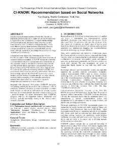
(a) #tracks per hour.

(b) Popularity of an artist.

Figure 1: Last.fm data information Furthermore, the music domain requires different techniques from the ones used for the movie or book recommendations. 1

http://www.last.fm

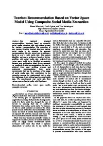
Figure 2: Rating distribution for the data set.

Users tend to listen to the same artist and track many times. Each user in our used data set on average listened for 5828.5 tracks. Repeated consumption of items enables us to analyze the users’ behavior in different conditions and compare the profile of the same user in various contexts (i.e. morning versus evening). Figure 1(a) shows listening behavior of all the users. The users are most active in the afternoon (4 p.m.) and least active early in the morning (5 a.m.). We also discovered that on average users tend to use more last.fm service during working days rather than during the weekends. Note that across the users some items are much more popular than others. Figure 1(b) shows by how many users the artist was listened at least once. Our goal is to build a time-aware RS that can accurately recommend an unknown and interesting artist (or a track) to the user. In our initial experiments we recommend an artist rather than a track, therefore, all the mappings here are done on the artist level. The ability to recommend a track will be proposed as a future work. To measure the performance of the system using the Mean Absolute Error (MAE) we map implicit user feedback into the explicit ratings. We then use Celma’s [4] proposed mapping procedure – that is similar to Hu et al.’s [6]. We take into consideration the number of times the user listened to an artist as an approximation of the users’ preferences. We assume that the more times the user has listened to an artist the more the user likes that particular artist. Note that user’ listening habits usually present a power law distribution, meaning that a few artists have lots of plays in the users profile, while the rest of the artists have significantly less play counts. Therefore, we compute the complementary cumulative distribution of artist plays in the users’ profile. Artists located in the top 80-100% of the distribution are assigned a score of 5, while artists in the 60-80% range assign a score of 4. In the case when there is not enough variation in the user profile to divide all the counts into 5 groups we assign 3 as the rating. Figure 2 shows the rating distribution for the data set. Note the fact that we have higher number of artists with small ratings. This is a specific property of the music data sets since a single user listens to a large amount of unique tracks or artists. This leads to many artists that the user has listened only once.

3.

APPROACH

Our long-term goal is to make a time-aware recommender system, which can accurately predict user’s music taste, given the current time. The overall vision is to represent a single user u by many micro profiles {u1 , u2 , ..., un } that

best represent the user in a particular time span. For example, we can have a representation of the same user u in the morning, evening, weekend, summer, etc. Micro-profiles would present a more precise model of the user. To make recommendations we would use multiple micro-profiles instead of a single profile u. The rationale behind the approach is that we can improve the accuracy while having a set of coherent and more precise user models. Micro-profiles for a single user can be built for many different time cycles (i.e. day, month or year). One of the main challenges, which we will not focus on this paper, is how to combine the predictions generated for each of the profiles and how to present the final predictions. But, even a more fundamental problem that we address, is how to discover meaningful time partitions based on the time cycles. Each partition should represent a time slice where user has similar repetitive behaviors. For example, the working hours of a user; if the user listens to the same set of artists while working. Each user could have different definition of the morning and the evening, therefore the same time partition might not work globally for all the users. For simplicity and evaluation issues (see Section 4), in this initial work we analyze only non overlapping partitions. Moreover, we evaluate our the system by making the predictions without combining several micro-profiles. Finally, we do not look into personalized partitions but rather evaluate global ones. We will address all of these issues as part of our future work.

4.

EVALUATION CHALLENGES USING IMPLICIT CONTEXT-ENRICHED DATA

The evaluation of a recommender system tries to estimate the users’ satisfaction for a given recommendation. The most common procedure is to use off-line evaluation techniques [5]. Different accuracy measure have been used to evaluate context-aware recommender systems (i.e expected percentile ranking [6], precision, recall, F1 [1], average precision [9]). Most of the previous work on CF evaluates the accuracy of the system using explicit user rankings [6]. In this Section we propose an off-line evaluation technique for implicit user ratings and continuous contextual variables. The biggest problem we tackle is closely related to the time

Figure 3: Examples of the partitioning T for a day. continuous contextual variable – in fact, the same evaluation problem generalizes to other continuous contextual variables such as temperature or distance to an object. To the best of our knowledge, this problem has not been addressed before

since most of the data sets contain ratings with a nominal contextual variable such as companion or weekday [1]. To understand the problem, imagine a scenario where a user is continuously listening to music. We want to build a system that is able to predict the user’s preference in various times of a particular day. Suppose the user likes two artists A and B. In the morning the user prefers artist A over B. On the contrary, at work the user prefers to listen to B more than A. When making a rating prediction for a specific time of the day, we should be able to infer these type of relations. Interestingly, the exact partitioning of the time domain defines the ground truth that we want to predict. For example, if we interpret “morning” as the time interval from 6 am to 9 am we will infer the users’ preferences by counting the popularity of the artist as described in Section 2. However, if we change the interpretation of morning, the users’ preferences might also change. Note, that these are the preferences we want to predict and not the predictions. In an off-line evaluation of the system, we compare the generated rating predictions to the hidden user ratings (holdout evaluation), serving as a ground truth. But because our ground truth depends on the exact partitioning of time, intuitively we need to take into account all the possible partitions. Furthermore, we need a success measure in order to decide, which partition is better. For this purpose, we propose to compute the error of the partition as the weighted average of all the errors in each segment: P |E(R, Ti , D) i |TiP E(R, T, D) = i |Ti | Where D is the data set, T = {T1 , T2 , . . . , Tt } is the time partitioning of the time domain. Partitions do not overlap and the union of them is equal to T . |Ti | is the number of the ratings we can predict in train set of the partition Ti . E(R, Ti ) is the Mean Absolute Error computed on the time partition Ti . The visual representation of possible partitioning is showed in Figure 3. Given the temporal partitioning T , the best system would be the one, which minimizes E.

5.

EXPERIMENTAL EVALUATION

For all of our experiments we used the last.fm data set described in Section 2. We used a popular factorization based CF algorithm (FACT for short)2 . Our testing approach for the Tday contextual segmentation is summarized in Figure 4. Due to the nature of implicit ratings, the procedure slightly differs from the usual off-line evaluation. In the initial step, the implicit data set of the user is subdivided into contextual segments defined by T . In the second step each of the segments is transformed into a user × item explicit rating matrix. We also transform the full data set into explicit ratings and divide it into the training and testing sets. To be able to compare the performance of different contextual segments we use the same test set for each of the segment. The user × item pairs in the test set is used to extract the test set for each of the contextual segments. All user × item pairs that are present in the test set and contextual segment are extracted to the test set of that particular segment. The rest of the ratings are assigned to the training set of the same segment. Note that we do not split each segment into 2

http://www.timelydevelopment.com

Figure 4: Example of testing aproach for morning and evening partitions. the training and testing sets independently from each other because some ratings we are trying to predict could already be present in the training set of the segment. This procedure also allows us to use the training set of one segment to predict the ratings in the test set of other segment.

5.1

Accuracy of the Method

Figure 5: Prediction accuracy for different segmentation. We shall now compare prediction accuracy of user microprofiling and our baseline (context-free) prediction algorithm. We use a pre-defined time segmentation, which was done for the day, the week and the year temporal repetition. Tday = {morning, evening}, Tweek = {weekend, working day}, Tyear = {cold season, hot season},Thours = {even hours, odd hours}. Morning is defined as day hours between 5 am and 6 pm. Hot season includes spring and summer in Spain (March 21st to September 21st). Even and odd hours represent the partitioning that was used to test the system behavior on the meaningless splits. The goal of the experiment is to test if we can improve the accuracy E of the predictor if we use only the profiles of the relevant segment. For example, for the day partitioning Tday we use only the user micro-profile of the morning to predict the ratings for the morning. We then compare the prediction accuracy E of this method against the prediction using the standard user profiles (without segmentation) to predict the user preferences in the morning and in the evening. For all the experiments we use five fold cross-validation. Figure 5 summarizes our results. The first column indicates the error E of the FACT CF predictor using user profiles without segmentation and making the prediction for the full user profile (without segmentation). This column plays the role for the base line to that other results are compared. The following columns show the performance of the algorithm when predicting user preferences defined by the partitioning T . The

algorithm makes predictions by taking into account users’ profiles without partitioning (marked “full” on x axis) or using only the users’ micro-profiles that of the corresponding segment (marked “seg” on x axis). The experiment shows how prediction accuracy improves when using more relevant user micro-profiles. Note, that accuracy dropped when predicting user preferences for the contextual segment using only a full users’ profile. It can be explained by the fact that in order to predict a specific users’ taste in the morning we use more general user data. On the contrary, when using only the data of the segment the prediction improved significantly. We observe the highest improvement for Tday and Thours partitioning. The improvement in Thours partitioning was unexpected and needs further analysis.

5.2

Similarities Between Splits

The previous experiment was conducted using pre-predefined time segmentations T . In our second experiment we aim at predicting the optimal split of the time variable. We examine the very simple case where the day cycle is partitioned into two segments each spanning for 12 hours. We want to find the optimal partition that reduces the overall error E. Figure 6 shows the true error E and the methods used to predict this error. On the y axis we plot the error (predicted error) E and on the x axis we plot the split point (i.e. every hour of the day). The graph is symmetric with respect to the gap of the 12 hours. This is because our time segment is 12 hours itself and the split at 0 o’clock is equal to the split at 12 o’clock. The true error is shown in the Figure 6(a). The error is computed every hour using the same prediction algorithm as in the first experiment. The minimum error in the day cycle is at 12 and 0 o’clock. We use different methods to predict the true error E. Figure 6(b) shows the estimation of the true error E using cross-validation. The cross-validation method is often used to estimate the free parameters of the algorithms. The split point could be seen as the parameter, which needs to be optimized with respect to the prediction error. We use 5 fold cross validation only on the train data – leaving out the test – to compute the E. Figure 6(b) shows, that the shape of the estimation resembles the shape of the true E. Note, that we try to predict only the optimal split point, therefore, we are interested only in the minimum points of the error and not in predicting the absolute value of E. Crossvalidation suggests that the minimum points are at 9 and 21 o’clock. The prediction is shifted to the left from the optimal solution by 3 hours. Note that using cross-validation to estimate the best split is expensive. It means running the recommendation algorithm several times for each possible split and this can be computationally unacceptable. Therefore, we compare this solution with two computationally cheaper methods. Both methods use proxy measures on the partitioned data set to compute the goodness of the split. The information gain (IG) method (see Figure 6(c)) uses this information theoretical measure to determine how much the split contributes to the knowledge of the data. We observe that the higher the information gain is, the smaller the error E. The maximum point is at 10 and 22 o’clock that is a closer prediction comparing to the cross-validation method. The third method computes the mean explained variance of the first 100 principal components for the two data segments. Similarly to the IG method, the more vari-

(a) True error E

(b) Cross-validation

(c) IG

(d) Explained Variance

Figure 6: Error and its estimation for different time splits. ance is explained by the smaller the error of E is. The most variance is explained at 9 and 21 o’clock, which leads to the same prediction as the cross-validation method. The experiment shows that predicting true error E for even the simple case can be a challenging task. Moreover, the well accepted cross-validation method can be outperformed by more lightweight heuristic approaches such as computing IG for the split.

6.

CONCLUSIONS AND FUTURE WORK

This work introduces and gives an initial evaluation of the micro-profiling technique for a time aware CF. We evaluated the method for different time splits and showed that using only the user micro-profile data for the prediction can actually increase the accuracy of CF. We also present a novel evaluation technique for context-enriched implicit data. Moreover, we compared three different methods to find the optimal partition of the data. The experiments showed how heuristic based methods can perform similarly good or out perform the more expensive cross-validation method. As part of future work we plan to make a more extensive evaluation of the micro-profiling approach. For initial evaluation we used user defined data splits. This has a limitation as the possible splits are predefined and do not depend on the data set or the user. We want to make more adaptive splits of the time domain. The split could be optimized for the entire data set or for each user separately. We expect to increase the accuracy of the current method. Moreover, we want to be able to combine the predictions made for different micro-profiles. For example, we could make a user micro-profile for weekends and for mornings, and compute the predictions for both of them. When predicting a rating for mornings on a weekend we should combine both predictions. The main challenge here is finding the precise way to aggregate different recommendations. In our initial experiments we made recommendations for particular music albums but not for music tracks. We want to extend our approach and make recommendations at different granularity levels, i.e., genre, artist, album and track. To the best of our knowledge this option has not been analyzed and could be useful for exploratory recommendations. In our work, we are considering only time as the context of the user. We want to extend the context information to include the current song along and the information of the current album. Note, that all of these extensions are very related

to our evaluation technique. The method we are proposing does not allow overlapping time partitions. Furthermore, the time partitions should be the same for all the users. In order to evaluate the method we would first have to find meaningful ways to compute the performance.

7.

REFERENCES

[1] G. Adomavicius, R. Sankaranarayanan, S. Sen, and A. Tuzhilin. Incorporating contextual information in recommender systems using a multidimensional approach. ACM Transactins on Information Systems, 23(1):103–145, 2005. [2] G. Adomavicius and A. Tuzhilin. Context-aware recommender systems. In P. Pu, D. G. Bridge, B. Mobasher, and F. Ricci, editors, RecSys, pages 335–336. ACM, 2008. [3] M. Anderson, M. Ball, H. Boley, S. Greene, N. Howse, D. Lemire, and S. McGrath. Racofi: A rule-applying collaborative filtering system. In Proceedings of COLA’03. IEEE/WIC, October 2003. [4] O. Celma. Music Recommendation and Discovery in the Long Tail. PhD thesis, Universitat Pompeu Fabra, Barcelona, Spain, 2008. [5] J. L. Herlocker, J. A. Konstan, L. G. Terveen, John, and T. Riedl. Evaluating collaborative filtering recommender systems. ACM Transactions on Information Systems, 22:5–53, 2004. [6] Y. Hu, Y. Koren, and C. Volinsky. Collaborative filtering for implicit feedback datasets. Data Mining, IEEE International Conference on, 0:263–272, 2008. [7] Y. Koren. Collaborative filtering with temporal dynamics. In KDD ’09: Proceedings of the 15th ACM SIGKDD international conference on Knowledge discovery and data mining, pages 447–456, New York, NY, USA, 2009. ACM. [8] O. Kwon and J. Kim. Concept lattices for visualizing and generating user profiles for context-aware service recommendations. Expert Syst. Appl., 36(2):1893–1902, 2009. [9] J. Lee and J. Lee. Context awareness by case-based reasoning in a music recommendation system. Ubiquitous Computing Systems, pages 45–58, 2008. [10] J. B. Schafer, D. Frankowski, J. Herlocker, and S. Sen. Collaborative filtering recommender systems. In The Adaptive Web, pages 291–324. Springer Berlin / Heidelberg, 2007.