{malex, jrg}@csail.mit.edu. ABSTRACT ... level of supervision required for designing and training a recog- ..... 2.96034 besides computer scientists deal with.
TOWARDS UNSUPERVISED PATTERN DISCOVERY IN SPEECH Alex Park and James R. Glass MIT Computer Science and Artificial Intelligence Laboratory 32 Vassar Street, Cambridge, MA 02139, USA {malex, jrg}@csail.mit.edu ABSTRACT
matic speech recognizers can only be trained, and have no capacity to learn from the data they observe following the training phase. In this paper we present a novel off-line approach to speech processing which attempts to address some of the shortcomings discussed above by minimizing supervision and dependence on prior knowledge. Rather than focus on the goal of recognition, we ask the question: “How much can be learned from the test data alone?”. Our approach is motivated by the growing body of tasks that utilize corpora such as academic lectures and personal audio archives. Among other common characteristics, these tasks can feature large amounts of data from a single speaker, esoteric vocabularies, and, in the case of classroom lectures, consistent acoustic environments. For these situations, real-time recognition is often not a requirement, but only a means to the end goal of being able to search, browse, and summarize the audio stream. With this in mind, we propose a departure from the “train-then-test” model of recognition and instead consider the problem of pattern discovery and sequence clustering in speech. The technique we discuss is inspired by related work in bioinformatics [1, 2], particularly comparative genomics. The goal of comparative genomics is to process massive amounts of genomic DNA or protein sequences to find patterns corresponding to genes, regulatory regions, and structurally important protein subsequences. Unlike speech, the lexicon of interesting subsequences is often not known ahead of time, so these items must be discovered from the data directly. Pattern discovery is made possible by the observation that functionally important biological sequences are more likely to be preserved across the genomes of different specimens than non-essential sequences. By aligning sequences to each other and identifying patterns that repeat with high recurrence, these preserved sequences can be readily discovered. Since there are a finite inventory of fundamental units that comprise a biological sequence – nucleic acids for DNA and amino acids for proteins – alignment reduces to simple string matching with penalties for insertion, deletion, and substitution. We can apply similar observations from comparative genomics back to speech. That is, patterns of speech sounds are more likely to be consistent within word or phrase boundaries than across. By aligning continuous utterances to each other and finding similar sequences, we can potentially discover frequently occurring words with minimal knowledge of the underlying speech signal. One possible approach is to transform the speech data into an intermediate representation resembling a biological sequence by using a phonetic recognizer to output a sequence of phone units. However, this type of translation is sensitive to the training data and units used in the phonetic recognizer. Instead, we describe an approach that uses a modification of dynamic time warping to directly compare utterances against each other at the acoustic level
We present an unsupervised algorithm for discovering acoustic patterns in speech by finding matching subsequences between pairs of utterances. The approach we describe is, in theory, language and topic independent, and is particularily well suited for processing large amounts of speech from a single speaker. A variation of dynamic time warping (DTW), which we call segmental DTW, is used to performing the pairwise utterance comparison. Using academic lecture data, we describe two potentially useful applications for the segmental DTW output: augmenting speech recognition transcriptions for information retrieval and speech segment clustering for unsupervised word discovery. Some preliminary qualitative results for both experiments are shown and the implications for future work and applications are discussed. 1. INTRODUCTION Modern speech recognition systems adopt a methodology in which most of the system parameters and settings are specified or learned in a highly supervised manner prior to testing or deployment. Although some systems use adaptation to adjust system parameters in response to the recognition input, recognition output is mostly determined by what is learned in the training phase. While this “train-then-test” model of recognition has led to steadily decreasing word error rates in the past, it has also resulted in systems that are vulnerable to different types of mismatch that constitute many of the difficulties faced by the ASR community. The out-of-vocabulary (OOV) problem is an example of mismatch caused by differences in the chosen lexicon and the set of words observed during testing. Inconsistent recognition performance for different speakers can be mostly attributed to the mismatch between the acoustics of speakers in the training data and the observed speaker. Even the phenomenon of speech recognizers hypothesizing English word sequences in response to foreign language speech can be classified as a mismatch issue. Additional sources of mismatch that can dramatically affect speech recognition accuracy include environmental conditions, speaking style, and language usage. Problems due to mismatch aside, there are more philosophical concerns with the “train-then-test” model of recognition. The level of supervision required for designing and training a recognition system is intuitively unsatisfying when one considers the ability of humans to learn spoken language without having access to labeled corpora of speech training data. For the most part, autoSupport for this research was provided in part by the National Science Foundation under grant #IIS-0415865.
0-7803-9479-8/05/$20.00 2005 IEEE
53
ASRU 2005
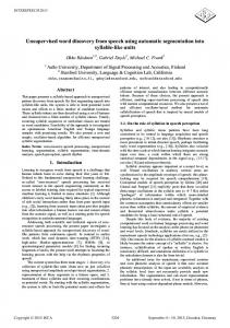
Utterance 1
without resorting to an intermediate symbolic representation.
U1
The remainder of the paper is organized as follows. In Section 2, we describe the segmental DTW algorithm which generates the best matching subsequence between two utterances. Next, we describe the data used in our experiments and outline the steps needed to process an entire audio lecture using the segmental DTW algorithm. In Sections 4 and 5 we propose two direct uses for our algorithm and show outputs for these preliminary experiments. Finally, we discuss several directions for future work and conclude.
Utterance 2
Distance Matrix
U2
2. SEGMENTAL DTW W
Dynamic time warping (DTW) is typically used to find the optimal global alignment between two whole word exemplars [3]. First, the two speech waveforms are converted into spectral vector time N series, {vi }M i=1 , {vj }j=1 . Next, a distance matrix D is computed by taking the pairwise distance between vectors in each utterance such that D(i, j) = �vi − vj �. Finally, dynamic programming is used to find the lowest distortion path through the distance matrix between D(1, 1) and D(M, N ).
Fig. 1. The segmental DTW algorithm. As in normal DTW, the distance matrix is computed between U1 and U2 . The matrix is then cut into overlapping diagonals (only one shown here) with width W . The optimal alignment path within the diagonal band is then found using DTW and the resulting path is trimmed to the least average subsequence. Finally, the trimmed alignment path is retained as the best subsequence alignment between U1 and U2 .
Recently, researchers have revisited the use of DTW for speech recognition as well as speaker detection [4, 5]. In the context of our work, the DTW algorithm is useful because it can be used to measure the similarity of two utterances directly at the acoustic level. However, performing a globally optimal alignment between two utterances is not suitable for finding matching words when those utterances are composed of multiple words. The start and end points constrain the algorithm to find only the globally optimal alignment matching the entire utterances together, and not local alignments which correspond to the matching subsequences.
3. EXPERIMENTAL DETAILS 3.1. Corpus The speech data used in this paper is taken from a corpus of audio lectures collected at MIT. The entire corpus consists of approximately 300 hours of lectures from a variety of academic courses and seminars. The audio was recorded using an omni-directional microphone in a classroom environment. In a previous paper, we described characteristics of this lecture data and performed preliminary recognition and information retrieval experiments [7]. Many aspects of the lecture data make it particularly well suited for the pattern discovery and speech clustering techniques described in this paper. Each lecture typically contains a large amount of speech (from thirty minutes to an hour) from a single person in an unchanging acoustic environment. On average, each lecture contained only 800 unique words, with high usage of subject-specific words and phrases. Each of the the lectures used in our experiments was the introductory lecture taken from courses in computer science (CS), physics, and linear algebra at MIT.
An alternative method to this global alignment procedure is to use segmental DTW, which finds local alignments by searching multiple paths in the distance matrix. Given two utterances, U1 and U2 , segmental DTW works by dividing the distance matrix into a set of overlapping diagonal bands with width W and searching for the best alignment within each band. The diagonal bands serve multiple purposes. First, they constrain the degree of warping so that two sub-utterances are not overly temporally distorted during alignment. Second, they allow for multiple alignments, as each band corresponds to another potential path with start and end points that differ from D(1, 1) and D(M, N ). Following path discovery, each path is trimmed by finding the least average subsequence with minimum length L. The minimum length criterion is used to prevent spurious matches between short segments within each utterance. Since each cell D(i, j) corresponds to the distortion between frames i and j, the least average subsequence represents the portion of the aligned path which exhibits good alignment. The algorithm used to compute the subpath is described in [6].
3.2. Preprocessing Prior to processing with segmental DTW, the lecture is segmented into continuous utterances by using a basic phone recognizer to identify regions of silence in the signal. Silent regions with duration longer than 2 seconds are removed and the portions of speech in between those silences are used as the input to the segmental DTW algorithm. In the absence of a phone recognizer, segmentation can also be performed using a speech activity detector. For the CS lecture processed in this paper, the segmentation phase resulted in 1946 segments averaging 1.2 seconds each. Each segment was then converted into a series of 14-dimension MFCC vectors extracted every 5 ms, then whitened using principal components analysis over all vectors from all utterances.
At this stage we are left with a single path fragment for each of the original bands in the distance matrix. The path fragment with the lowest average distortion is retained as the best alignment path between the two utterances, and this minimum average distortion is used as the distance between U1 and U2 . This alignment path along with its associated distortion forms the basis for further processing that we will describe in the following sections.
54
Query Utterance
Lecture Timeline
well are very unlike parentheses in conventional mathematics
Silence Detection Segmented Utterances
1
2
3
Nearest Neighbours
4
2.67685 and it sort of doesn't hurt if sometimes you leave out parentheses if people understand that that's a group 2.71682 and in general it doesn't hurt if you put in extra parentheses 2.73775 flashing parentheses 2.76504 right because putting in parentheses always mean 2.84133 in lisp you cannot leave out parentheses 2.86766 you see the parentheses close close the minus 2.89815 close parentheses which is going close the 2.90602 well 3.00560 that looks very much like the case analysis you use in mathematics
Segmental DTW Alignment Paths
1
2
3
4
Fig. 2. Audio processing for segmental DTW. Silence detection is used to break the original audio stream into smaller utterances. The utterances are then compared against each other using segmental DTW to produce alignment paths. The alignment paths match a segment from one utterance to a segment in another utterance together with a distortion measure for that path.
Fig. 3. An example of an actual acoustic query. Transcriptions of the query utterance and its nearest neighbours are included for illustrative purposes only. The numbers in the lefthand column are the average distortion measures for the alignment path between the query and the returned result. Words common to both utterances within the alignment path are shown in bold.
3.3. Path detection using segmental DTW Once MFCC feature vectors have been extracted, we compute common paths between each utterance using segmental DTW. In this phase, each utterance is compared against each other utterance. For our experiments, we set the parameters W and L to be 15 (75 ms) and 100 (500 ms), respectively. These values were selected somewhat arbitrarily but seemed to yield acceptable results. Further experiments may yield more optimal settings. One concern regarding this stage of processing is that performing path detection over all pairs of utterances might be computationally prohibitive. In practice, however, we have observed that the amount of time required for processing the comparisons on one hour of speech is roughly the same as performing recognition with a large vocabulary recognizer. Moreover, because each pairwise comparison is independent of the other comparisons, the entire computation can be easily parallelized for further gains. The only major computational drawback of our method is that performing a global set of comparisons necessitates off-line processing. However, in an on-line scenario, the results of incremental comparisons can be obtained by processing utterances as they are received.
to perform information retrieval on the lecture with a set of keywords and phrases taken from the index of the course textbook [7]. With the segmental DTW system, it is difficult to generate comparable statistics. However, we can still evaluate the utility of our algorithm by considering the incremental benefits that it may offer to the recognition based information retrieval system when the two are combined together. We illustrate one possible augmentation strategy using queries where the recall rate using the recognition-based IR system is less than 100 %. These query terms, along with their recall rate, and missed instances, are shown in Table 1. For each query, we can incorporate the output of our segmental DTW algorithm by ranking all lecture utterances by their average similarity to the found results. We can see from the table that in most cases, the missed results rank quite highly as neighbours of the found results when using acoustic similarity. The wide variability of the recognition hypotheses for the missed instances also highlight the difficulty of trying to recover these results from the transcription alone. While further experiments are necessary to determine how our approach can be used globally to improve recall while minimizing the effect on precision, we can see that acoustic similarity scoring is beneficial because of the added flexibility it offers. During search for a particular query term, we can easily expand the search beyond the recognition results to get a ranked list of candidates without having to rely on multiple word hypotheses or confidence scores.
4. ACOUSTIC SIMILARITY FOR LECTURE BROWSING The output of the segmental DTW algorithm can be thought of as an undirected adjacency graph, with utterances representing the nodes, and the alignment paths between utterances representing the edges. In this graph, the average distortions associated with each alignment path are a natural analogue to edge weights, with lower distortion edges corresponding to more similar utterances. Left as is, the adjacency graph can be useful for browsing through audio lectures by providing pointers to portions of the lecture that are acoustically similar to the current playing utterance. Using the current utterance as a query, nearby nodes in the graph can be thought of as acoustically relevant segments in the lecture. Two query examples and their associated outputs are shown in Figure 3 and 4. For both examples, each of the nearest neighbours contains at least one word in common with the query utterance. Though useful for browsing, substituting utterances as queries does not fit well with traditional models of evaluation for information retrieval. In previous work, we used recognition transcriptions
5. GRAPH CLUSTERING FOR WORD DISCOVERY The adjacency graph described in the previous section connects multi-word utterances to each other. Initially, we had planned to use graph clustering techniques to discover words by finding densely connected groups of utterances. The main difficulty with our proposed idea can be illustrated using the example in Figure 3. Because the query utterance contains multiple words, there are also multiple ways in which each query can match its neighbours
55
Query Utterance and it's not about computers in the same sense that
3
Nearest Neighbours 2.83921 now the reason we think computer science is about computers 2.85811 or we'll actually see that computer 2.87800 the essence of computer science 2.93215 sense that geometry 2.93642 computers in the same set 2.95375 and the real issues of computer science are of course not 2.96034 besides computer scientists deal with 2.97730 that computer science in some sense 3.03468 what do i mean by the essence of computer science what do i mean by the essence of geometry
absolute value
6/8
abstraction
8/16
black box fixed point
5/7 12/14
Cluster Rank 1 2 1 2 3 5 6 7 9 15 1 2 1 21
1
9
5 6
8
Fig. 5. An example illustrating the soft clustering problem that results from using utterances as nodes in the adjacency graph. Utterance 1 has words in common with all other nodes shown, with clusters {1,2,3}, {1, 4, 5, 6}, and {1,7,8,9} corresponding to different words. If utterances 2 and 4 also shared a common word, the graph becomes difficult to separate.
Recognition Hypothesis us to tell you drafted guidelines and check and and track and for traction subtraction subtraction interaction stretch instruction like rock like bach takes point exp one
Inverse Distortion
Recall Rate
4
7
Fig. 4. Query results for a second example as in Figure 3. Keyword
2
Piled intervals Smoothed version Detected peaks
Time
Fig. 6. The node refinement process. The solid line indicates the inverse distortion (similarity) profile generated by aggregating alignment paths for this segment of time. The dashed line is the result of smoothing the similarity profile with a triangular window. The refined node locations, which are found by picking peaks from the smoothed profile, are indicated by circles.
Table 1. Query terms with less than 100 % recall rate. For each term, the missed instances are listed, along with their cluster rank and the recognition hypothesis for that particular term. The cluster rank is found by sorting all non-returned utterances by their average acoustic similarity to returned results.
semblance to locations within other utterances. First, we collect all alignment paths falling under an average distortion threshold and aggregate the inverted distortions to form a similarity profile within the utterance. After smoothing the similarity profile with a triangular averaging window, we take the peaks from the resulting smoothed profile as the refined nodes. The refinement process is shown and explained in Figure 6. The reasoning behind this procedure can be understood by noting that only some portions of any particular utterance have high similarity (i.e. low distortion) to other utterances. By focusing on the peaks of the aggregated similarity profile, we restrict ourselves to parts of the utterance that are most similar to other utterances. Since every alignment path covers only a segment of the utterance, the similarity profile will fluctuate, allowing the utterance to separate naturally into multiple nodes corresponding to different word identities. Edges in the refined adjacency graph are given by the alignment paths that overlap the time index of a particular node. Figure 7 illustrates how breaking utterances into refined nodes can potentially aid word level clustering.
in the adjacency graph. Although the majority of returned results contain the word “parentheses”, there are also results matching the words “well” and “mathematics”. Expanding our view to consider edges between the returned results as well, we can easily imagine situations like the one shown in Figure 5, where a single utterance belongs to multiple clusters, each one corresponding to a different word. Thus, if we use only edge weight information, the graph clustering problem remains a difficult soft clustering problem. Our solution is to use the locality of the alignment paths to generate a refined set of nodes from the original group of utterances. 5.1. Node refinement In the node refinement stage, we extract a set of time indices from each utterance and use those indices as refined nodes. The refined indices demarcate locations within an utterance that bear re-
56
3
2
procedure procedure procedure
square square
4
7
square
9
procedures procedure procedure procedure
square
procedure procedureprocedure procedure
square
5
1
procedures
square square square
square square square square square
8
computers computer computer computer computer computer computer science
6
Fig. 7. The same example as in Figure 5, but with utterance nodes broken into refined nodes. Refinement eliminates the problem of the same node belonging to multiple clusters because each refined node represents a single time index.
procedure
procedures procedures procedures
procedure procedure procedures procedures procedures
computer computer science computer procedures procedures
computer science
procedures
procedures
(a) A computer science lecture. 5.2. Word cluster output electricity
Once the utterance level nodes have been refined into time index nodes, we can generate an adjacency graph by pruning away edges that are above a specified distortion threshold. With a pruning threshold that keeps only the lowest 5 % of edges by distortion, a relatively sparse graph can be produced which can be extremely useful for visualization and word discovery. In Figure 8 (a), three of the larger connected components of the adjacency graph are shown. The nodes in the graph are labeled with the actual word (or words) that overlap the node time index, but these labels were not used at any point in the generation of the adjacency graph. These connected components are found solely based on the consistency of the underlying acoustic sequences and can therefore be thought of as patterns discovered by simply comparing speech utterances against each other. In the majority of cases, the nodes in connected components point to the same underlying word. Figures 8 (b) and (c) show similar sets of connected components that were extracted using the same procedure on lectures from two different subjects. At first glance, the component labels seem to have a high degree of relevance to the subject material. In Table 2, we attempt to examine the relevancy of the clusters from the computer science lectures more thoroughly. The top connected components with at least 6 nodes are listed, sorted in order by their cluster density. The cluster density, which is given by the percentage of edges that exist between the nodes of a cluster out of the number of possible edges, offers a measure of reliability for each connected component. The lecture examined here consists of an example-based introduction to Lisp programming using arithmetic functions. In order to examine the relevancy of some of the terms found using our method, Table 2 also includes the frequency rank of each term in the lecture (with common words removed). Although several of the clusters correspond to common words, the majority of the clusters correspond to highly relevant terms, with six of the terms occuring in the top ten most frequent lecture words. Frequently occuring lecture words that are not listed in the table include: “lisp”, “define”, “primitive”, and “language”. Our description of this word clustering technique is certainly not intended to be an exhaustive treatment on the problem of word discovery. Many aspects of the algorithm can be improved upon or explored in a deeper manner. For example, we currently rely on graph components being separated in order to find word groups. This approach necessitates a distortion threshold in order to re-
electricity electricity
induction
induction
electricity induction electricityelectricity induction electricity electricity electricity electricityelectricity conductor electricity electricity conductor conductor electricity electricity electricity electricity conducted conductor electricity electricity conductor
(b) A physics lecture on electricity and magnetism. column matrix
the matrix
column column column
matrixmatrix matrix matrix matrix matrix matrix
extra matrix
matrix
matrix matrix matrix matrix matrix
matrix matrix matrix
matrix matrix
columns
columns
matrix columns column column
matrix
columns columns
column columns
columns
columns columns
(c) A mathematics lecture on linear algebra. Fig. 8. Several connected components of the adjacency graphs for different academic lecture generated by retaining a small percentage of edges connecting the refined nodes. The nodes are labeled according to the words overlapping the node time index for reference purposes only. (The threshold used for the adjacency graph in (a) differs from that used for Table 2)
move edges and produce a sparse adjacency graph. In addition to pruning nodes and edges from each of the clusters, it also discards edge weight information. A more sophisticated graph clustering algorithm will eliminate the need for a distortion threshold and allow us to use the edge weights directly in the clustering process. Despite the simplicity of our clustering algorithm, however, the purity of the groups shown in Table 2 and their relevance to the lecture subject material is encouraging.
57
Cluster Label definition square five combination product average value parentheses computer that procedure reduces square root for/four about
Density (%) 100.0 94.9 93.3 93.3 92.9 87.9 86.6 81.8 80.0 80.0 76.7 60.0 59.5 53.0 51.5
Size 6 13 6 6 8 12 6 11 15 6 33 6 68 12 22
Purity (%) 100.0 100.0 100.0 100.0 100.0 100.0 100.0 100.0 100.0 83.3 100.0 66.7 89.7 66.7 90.9
Rank 21 1 10 33 11 6 15 6 5 94 2 -
how pattern discovery can be used for music summarization and multimedia retrieval [8, 9]. In those works, direct acoustic comparison was used to successfully extract the chorus from a song by looking for repeating themes and melodies across time. Likewise, we can envision generating direct audio summaries by simply playing back instances of the salient words found by clustering. 7. CONCLUSION In this paper, we have presented a simple, unsupervised technique for processing speech using a variation of dynamic time warping. By performing pairwise comparisons on a set of segmented utterances, we have demonstrated how direct acoustic comparison can be useful for augmenting speech recognition in information retrieval. Of more interest, perhaps, we have shown how the same procedure can be useful for discovering words and phrases directly from speech. The underlying insight behind our approach is that word and phrase information is inherent in speech data in the form of repeating occurrences of acoustic patterns. By aligning these patterns, we can potentially identify which patterns correspond to the same underlying words. Although our results at this stage are mostly qualitative, we believe that these results have promising implications for a variety of problems in speech research.
Table 2. List of connected components in the thresholded adjacency graph for the computer science lecture. The cluster label is determined by the label for the majority of the nodes. The purity of the cluster is given by the percentage of nodes whose label agrees with the cluster label. The density of the cluster is given by the percentage of edges that exist between nodes out of the number of possible edges. The rank column indicates the frequency rank of the word(s) in the lecture after removing the 300 most common words from Switchboard.
8. REFERENCES [1] I. Rigoutsos and A. Floratos, “Combinatorial pattern discovery in biological sequences: the TEIRESIAS algorithm,” Bioinformatics, vol. 14, no. 1, pp. 55–67, February 1998.
6. FUTURE WORK
[2] A. Brazma, I. Jonassen, I. Eidhammer, and D. Gilbert, “Approaches to the automatic discovery of patterns in biosequences,” J. Computational Biology, vol. 5, no. 2, pp. 279– 305, 1998.
Our goal in this paper has been to simply introduce the segmental DTW algorithm and show how the unsupervised nature of this algorithm makes it suitable for several applications in speech processing. Some specific applications are discussed below. One of the most promising directions for future work concerns the problem of word discovery, which we touched upon in Section 5. Ultimately, we would like to find pure clusters of different instances of the same underlying word, and exploit latent consistencies to construct a robust representation of that word. Such a technique would be immensely useful for speech recognition, and could also provide insights into the problem of language acquisition. More immediately, there are several ways that we can improve the node refinement and clustering procedures discussed in Section 5. Instead of relying on time indices alone, we may be able to extract word boundaries by repeating the segmental DTW process on node neighbourhoods. As mentioned earlier, we can use more powerful graph clustering algorithms to find word clusters without requiring total separation in binary adjacency graphs. Following upon the experiment discussed in Section 4, we plan to examine how segmental DTW clusters can be used in combination with a conventional speech recognizer. Since recognition is typically performed in a very localized manner, automatic systems do not exploit the consistency constraints that exist between multiple utterances of the same word. The clusters generated by our algorithm can act as a secondary knowledge source which identifies these multiple instances. Consistency can then be enforced using, for example, a voting scheme that ensures cluster members have word hypotheses that agree with each other. Finally, speech summarization is another area that can benefit from segmental DTW. Several researchers have already shown
[3] L. Rabiner and B.H. Juang, Fundamentals of Speech Recognition, Prentice Hall, 1993. [4] M. De Wachter, K. Demuynck, D. Van Compernolle, and P. Wambacq, “Data driven example based continuous speech recognition,” in Proc. Eurospeech, Geneva, 2003, pp. 1133– 1136. [5] D. Gillick, S. Stafford, and B. Peskin, “Speaker detection without models,” in Proc. ICASSP, Philadelphia, 2005, pp. I–757–760. [6] Y-L. Lin, T. Jiang, and K-M. Chao, “Efficient algorithms for locating the length-constrained heaviest segments with applications to biomolecular sequence analysis,” J. Computer and System Sciences, vol. 65, no. 3, pp. 570–586, January 2002. [7] A. Park, T. J. Hazen, and J. Glass, “Automatic processing of audio lectures for information retrieval: Vocabulary selection and language modeling,” in Proc. ICASSP, Philadelphia, 2005, pp. I–497–450. [8] C. Burges, D. Plastina, J. Platt, E. Renshaw, and H. Malvar, “Using audio fingerprinting for duplicate detection and thumbnail generation,” in Proc. ICASSP, Philadelphia, 2005, pp. III–9–12. [9] J. Foote, “An overview of audio information retrieval,” J. ACM Multimedia Systems, vol. 7, no. 1, pp. 2–10, 1999.
58