complex applications using MMS. By S. P. Dominoâ . A novel numerical algorithm is presented that allows for efficient coupling of non- conformal mesh blocks in ...
Center for Turbulence Research Proceedings of the Summer Program 2010
167
Towards verification of sliding mesh algorithms for complex applications using MMS By S. P. Domino† A novel numerical algorithm is presented that allows for efficient coupling of nonconformal mesh blocks in both static and non-static (sliding) low Mach number fluids applications. The algorithm combines use of the finite element method (FEM) at interior domains with a discontinuous Galerkin (DG) implementation at the nonconformal mesh interface. The mixed FEM DG algorithm is applied to a recently implemented FEM-based core fluids algorithm that uses equal-order pressure stabilization and residualbased advection stabilized methods; details of this stabilized algorithm are presented and a test suite of simulations is compared against a control volume finite element method (CVFEM) implementation. A set of formal verification solutions, including the method of manufactured solutions (MMS), are introduced to verify the second-order accuracy of this new method. Two test simulations are presented to evaluate the capability for equal-order pressure stabilized flows with a both static, nonconformal meshes and dynamic sliding grids. The former represents a T-duct flow simulation with the nonconformal interface across a re-circulation zone. The latter demonstrates multiple rotating domains in the context of a sliding mesh application.
1. Introduction Dynamic sliding mesh simulations are required in several engineering applications such as wind turbine analysis and require an efficient implementation of nonconformal mesh joining. A variety of capabilities to handle such mesh configurations exist and include finite element-based multipoint constraint methods (Gartling 2005), interface capture and tracking methods (Tezduyar 2001) and cell centered finite volume methods (CCFVM) in which a flux matching protocol is employed (Lilek et al. 1988), where care is required to reconstruct a conservative area representation between the two blocks (Moen et al. 2000). However, an alternative method which has been successfully used in finite elementbased thermal applications has recently been developed at Sandia National Labs for complex heat transfer applications (Shakib 2005) and implemented within the Sierra/T H code base. This methodology combines the FEM within the interior elements and DG methods at the nonconformal mesh interface. A complete and formal description of the methodology, with test problems and verification for heat conduction applications with and without contact resistance, can be found in the SAND report by Carnes & Copps 2008. Compared to other first-order spatial methods, this generalized approach for nonconformal mesh interfaces has been proven to be second-order accurate for linear elements and robust. The primary goal of this paper is to extend the FEM and DG nonconformal method for equal-order pressure stabilized low Mach number fluids applications. The method of † Computational Thermal and Fluid Mechanics, Sandia National Laboratories
168
Domino
Figure 1. Two-block example with one common surface, ΓAB .
manufactured solutions (Roache 2002) is used to verify the second-order accuracy on nonconformal meshes. The MMS provides a high-quality metric to determine code correctness as the order of accuracy can be precisely determined using an exact solution. The secondary goal of this paper is to provide a detailed overview of the equal-order pressure stabilization and residual-based advection stabilization used for low Mach number flow calculations. Towards this end, theory, verification and test cases that compare the newly implemented formulation against previous CVFEM studies are provided. Massively parallel simulations integrating high-fidelity coupled physics are provided through the Sierra Mechanics code project (Edwards 2006) and more recently, the Sierra T oolkit project (Edwards et al. 2010). The Sierra Mechanics project is funded through the Advanced Simulation and Computing (ASC) Program, which is a NNSA funded initiative to support science-based stockpile stewardship. The Sierra T oolkit provides core services for parallel computing via a variety of solver, assembly and mesh transfer services (Williams 2004). The code base into which this feature is implemented is the consolidated Sierra/F D code base, which is based on the ARIA code (Notz et al. 2005).
2. Algorithmic Description for Simple Diffusion Consider two domains, A and B, which have a common interface, ΓAB , and a set of interfaces not in common, Γ\ΓAB (see Figure 1), and assume that the solution of the time-dependent diffusion equation for the mixture fraction Z is to be solved in both domains. Each domain has a set of outwardly pointing normals. In this cartoon, the interface is well resolved , although in practice this may not be the case. The transient diffusion equation with general source, S, ∂ρZ ∂qj + = S, ∂t ∂xj
(2.1)
where ρ is the density and the flux vector, qj is qj = −ρD
∂Z . ∂xj
(2.2)
Finally, D is the mass diffusivity. The numerical description follows the unified approach of Arnold et al. (2002). Specifically, the variational equation includes the notation of averages and jumps at the boundaries. For a scalar quantity like Z, the following notations are defined:
Towards accurate sliding mesh algorithms
169
1 A (Z + Z B ), 2 B B [[Zj ]] = Z A nA j + Z nj . hZi =
(2.3) (2.4)
Note that if Z is a scalar, hZi is a scalar and [[Zj ]] is a vector. For a vector qj , the average and jump are defined as follows: 1 A (q + qjB ), 2 j B B [[q]] = qjA nA j + q j nj . hqj i =
(2.5) (2.6)
Note that hqj i is a vector and [[q]] is a scalar. The variational statement for both domain A and B is obtained by multiplying Eq. (2.1) by an arbitrary test function w that is continuous within each domain; however, it can be discontinuous across the shared interface, ΓAB . Here, the diffusional partial differential equation term is integrated by parts. Using the jump and average notation, and following a classic interior penalty method for boundary fluxes at the ΓAB interface, the following variational equation is obtained: �
Z w
� Z Z ∂ρZ ∂w − S dΩ − qj dΩ + ∂t ∂xj Ω
Ω
Z + ΓAB
Z [[wj ]]hqj idΓ − ΓAB
∂w hρD i[[Zj ]]dΓ + ∂xj
wqj nj dΓ
Γ\ΓAB
Z λ[[wj ]][[Zj ]]dΓ = 0.
(2.7)
ΓAB
Note that the first equation line represents the standard Galerkin FEM terms while the second line includes the new DG terms. In accordance with the standard Galerkin method, solutions to the weak statement lie in a differentiable space of functions. Moreover, the standard basis functions are Lagrange polynomials with coefficients provided at the nodes of the mesh. As noted in the Arnold paper, the interior penalty method has been proven to be both consistent and stable. Note that the fifth term in the above equation includes a gradient of the test function that requires one layer of elements at the nonconformal interface. This term was not included in the first algorithm (Carnes & Copps 2008); however, preliminary results (see section 2.1) indicate that inclusion of this term for the diffusion-only test case slightly decreases the error norms and does not appreciably affect nonlinear convergence. However, in generalized fluids problems, inclusion of this term in the continuity equation, Eq. (5.2) and Eq. (5.3), has been found to be of critical importance. Above, the parameter λ is computed as the ratio of an average diffusive flux coefficient and a local mesh size that is based on each connecting element (Carnes & Copps 2008). Although the Arnold procedure is useful in defining a common interface by which all DG methods can be analyzed, we introduce an alternative description and write the variational equation for each domain with a notion of numerical fluxes defined at the DG interface. The simple model diffusion equations written in terms of numerical fluxes for domain A and B are
170
Domino Z
wA
�
ΩA
� Z Z ∂ρZ ∂wA − Si dΩ − qj dΩ + wA qj nj dΓ ∂t ΩA ∂xj Γ\ΓAB Z ˆ n (A, B)dΓ + wA Q
(2.8)
ΓAB
Z + ΓAB
∂wA nj λIP (Z A − Z B )dΓ, ∂xj
and Z ΩB
wB
�
� Z Z ∂ρZ ∂wB − Si dΩ − qj dΩ + wB qj nj dΓ ∂t ∂x j ΩB Γ\ΓAB Z ˆ n (B, A)dΓ + wB Q
(2.9)
ΓAB
Z + ΓAB
� ∂wB nj λIP Z B − Z A ) dΓ. ∂xj
ˆ n (α, β), are The numerical fluxes, Q h i β β α β ˆ n (α, β) = 1 (qjα nα Q − q n ) + λ(Z − Z ) . j j j 2
(2.10)
2.1. Steady, Diffusion, Static Mesh Manufactured Solutions Verification The manufactured solution used to test the model scalar diffusion FEM/DG implementation is taken from Domino 2008. The culmination of this study was to present a fully coupled equal-order pressure stabilized formulation and demonstrate the second-order spatial accuracy of the method using modifications of classic Taylor Vortex first presented by G. I. Taylor (Taylor 1923). The manufactured solution used in this simple model diffusion equation is based on the formal pressure solution, Zo (cos(2aπx) + cos(2aπy)), (2.11) 4 where the constant a controls the number of wave amplitudes within the domain of interest. Figure 2 represents a converged result for the coarse mesh; shown are both the mesh and the shaded values of mixture fraction. In this study, the mesh was rotated to provide the most difficult location in which the nonconformal mesh interface resides (determined by picking the highest value of the L∞ norm). Table 1 provides the L∞ norms for the mixture fraction, Z, over three mesh refinements using the interior penalty algorithm. Results verify that, as expected, the mixed method algorithm is second-order accurate as the residual reductions for a uniformly refined mesh ∂w is a factor of four. Note that when omitting the term hρD ∂x i[[Zj ]], the coarse value norm j is 0.0243 and no appreciable nonlinear convergence degradation is detected. Z(x, y) = −
3. Nonconformal Code Implementation The code implementation for the calculation of numerical fluxes at the nonconformal interface is somewhat straightforward. The procedure first involves identifying current
Towards accurate sliding mesh algorithms
171
Figure 2. Shaded plot of the variable Z with the mesh lines outlined.
Variable Z
L∞ Residual Norm decreasing ∆x sets ⇒ 1.986211e-3 4.99048e-4 1.24450e-4
Table 1. Residual norms for mixture fraction, Z, as a function of mesh spacing.
and opposite integration points for a pair of surface:parent elements for both the A : B and B : A block pair. An efficient geometric search is used to determine the set of elements required for numerical flux evaluation at the current and opposite integration points. The opposite integration point location is simply determined by a geometric projection. Next, the current and opposite isoparametric coordinates along with the appropriate surface:parent elements are provided to an algorithm assembly method. Figure 3 graphically demonstrates the procedure in which integration point values of ϕ are computed on the block A surface and at the projected location of block B. In the cited figure, this mapping of integration points and projected value are given by ϕ˜A ˜B ip and ϕ ip . Should the DG terms require fluxes, gradients are computed based on the surface:parent element pair for each face using the standard finite element shape function derivatives. Average fluxes are computed based on the current and opposite integration point locations. The appropriate DG terms are assembled as boundary conditions first with block A integration points as current (integrations points for block B are opposite) and then with block B integration points as current (surfaces for block A are, therefore, opposite).
4. FEM Stabilized Low Mach Number Algorithm This section describes the equal-order pressure stabilization and provides three test cases to compare the finite element results to the control volume finite element set of results. In general, this outlined formulation is based on the generalized, fully coupled pressure stabilization approach outlined in Domino 2008; however, it is now directly applied to the finite element discretization. (For a detailed overview of the methodology and how it relates to a class of stabilized pressure schemes, the reader is referred to Domino 2006 and Domino 2008). The use and evaluation of this pressure-stabilized method applied to a finite element methodology is a requisite step as the proposed non-conformal mesh algorithm is finite element-based. Although this method of pressure stabilization dates back to Rhie and Chow in the context of collocated finite volume schemes (Rhie & Chow 2002), the method follows closely the formal class of stabilization methods known as
172
Domino
Figure 3. Description of the numerical flux calculation for the DG algorithm. The value of ϕ on the current block (A) and the opposite block (B) are used for the calculation of numerical fluxes. ϕ ˜ represents the projected value.
local projection stabilization, e.g., see Braack et al. (2009) which leverages other foundational work to extract the positive attributes from a range of discretization/stabilization approaches (Codina 2001). Finally, the algorithm is presented in the context of a fully coupled methodology although the transformation to a pressure projection scheme is readily applied (again, see Domino 2008 for a lengthy description). The equal-order stabilized continuity is derived by multiplying the general variable density continuity equation, ∂ρ ∂ρuj + = S, ∂t ∂xj
(4.1)
by the test function v and integrating the advection term by parts. Applying the pressure stabilization algorithm, the resulting equation is �
Z v Ω
� Z Z ∂v ∂ρ − S dΩ − ρuj dΩ + vρuj dΓ ∂t ∂xj Ω Γ � � Z X ∂v c c ∂p − γτ Gj p − τ dΩ ∂xj ∂xj elem Ω � XZ � ∂p nj dΓ = 0, + v γτ c Gj p − τ c ∂xj open
(4.2)
Γ
c
where τ is the stabilization time scale for the continuity equation, Gj p is a projected pressure gradient (see Eq. (4.3)) and the parameter γ controls the continuity equation error which is proportional to either the second derivative of pressure (γ = 0) or the fourth derivative of pressure (γ = 1). Note that pressure stabilization contributions at surface elements are germane only when open pressure-specified boundaries are present. As a brief review, the essential attribute of this pressure stabilization is due to a ∂p , and the nodally scaled difference, τ c , between the local elemental pressure gradient, ∂x j projected pressure gradient, Gj p. The stabilzation error, as noted above, is either proportional to the second or fourth derivative of pressure. The parameter τc is a time scale that is either related to the time step, advection and diffusion time scale, or a combination of both (Domino 2006).
Towards accurate sliding mesh algorithms
173
The pressure gradient is obtained by a local projection equation that can either be lumped or determined by using a consistent mass matrix, Z Z Z ∂w wGj pdΩ + pdΩ − wpnj dΓ = 0. (4.3) ∂xj Ω
Ω
Γ
Moreover, the projection equation can either be fully coupled, lagged in time or lagged within the nonlinear iteration Picard loop (effectively computing the nodal gradient just before the fully coupled continuity and momentum system). The discrete momentum equation is also obtained by the standard finite element variational approach. The momentum equation, ∂ ∂ρui + (ρuj ui − σij ) = Si , ∂t ∂xj
(4.4)
is multiplied by the test function, w, and integrated over the domain. For the momentum equation, both the stress and advection are integrated by parts. Above, the Cauchy stress, σij , is given by 2 ∂uk δij . σij = τij − pδij + µ 3 ∂xk
(4.5)
Here, the advection stabilization methodology known as streamwise upwind PetrovGalerkin method (SUPG) is used (see the classic paper, Brooks et al. 1982, and more recently, Hsu et al. 2010 for a good overview of the technique). �
Z w Ω
� Z Z ∂ρui ∂w − Si dΩ − (ρuj ui − σij ) dΩ + w (ρuj ui − σij ) dΓ ∂t ∂xj Ω Γ � X Z ∂w � ∂p − γτ c Gj p − τ c + ui dΩ ∂xj ∂xj elem Ω � � XZ c c ∂p + w γτ Gj p − τ ui nj dΓ ∂xj open Γ � � XZ ∂w ∂ρui ∂ρuk ui ∂p m + τ uj − Si + + = 0. ∂xj ∂t ∂xk ∂xi
(4.6)
elem Ω
In the above equation, the first line represents the standard FEM discretization. The second and third lines represent the pressure stabilization terms carried through to the momentum equation within the interior of the domain and at open boundaries. The fourth and final line represents the residual-based advection SUPG stabilization. Above, τ m represents the advection stabilization time scale (see Hsu et al. 2010 for details). Note that the viscous stress tensor contribution is omitted from the full momentum residual within the SUPG contribution. Also of interest is the choice to integrate the Galerkin advection term by parts while allowing the SUPG momentum residual contribution to be in divergence form. Finally, the pressure stabilization term follows through to the momentum equation to account for the fact that there is discrete error due to the continuity equation. The inclusion of the pressure stabilization terms to augment the standard mass flux vector, ρuj , has its classic roots in the work of Majumdar (1988). Specifically, note that the advection term in the first line of Eq. (4.6) can be combined
174
Domino
Figure 4. Variable density steady Taylor vortex L∞ norm; FEM (L) and CVFEM (R).
with the pressure stabilization term in line three to form a numerical advection flux, ρu ˆj. 4.1. FEM and CVFEM Algorithmic Comparison This subsection provides three numerical test comparisons between FEM and CVFEM. The first comparison simulation study represents a manufactured solution with formal orders of accuracy compared. The second comparison study represents a laminar open jet (Reynolds number of 36). Finally, the third test case is a classic laminar backward facing step which is near the transition to a turbulent flow (Reynolds number of 1200 based on step height). In this paper, the objective is not a validation study. As such, comparison to experimental data is not reported. The prime objective of the second and third test case is to compare the methods on a given mesh. However, details of the validation study for the open jet and backward facing step can be found in Luketa & Domino (2010). The first test case presented parallels the high-quality variable density low Mach number verification test suite outlined in Domino 2008, using the method of manufactured solutions. The manufactured solution is a modifed steady Taylor vortex analytical solution to include variable density flow via a coupled mixture fraction equation. Not shown are the pressure gradient norms which are observed to be first order in the L2 norm. Figure 4 outlines two convergence plots for FEM (L) and CVFEM (R) using fourthorder pressure stabilization. The results show that each method is second-order accurate in the L∞ norm for mixture fraction and velocity. Moreover, it can be seen that the magnitude of error norms between the two methods are extremely comparable. The second comparison test problem represents a simple laminar open jet (Reynolds number of 36) based on an inlet jet dimension of 0.0072 meters. In this simulation, the inflow boundary condition is enclosed by open boundaries with constant total pressure specification. Figure 5 represents a comparison of streamwise velocity as a function of axial distance for the second-order pressure stabilization algorithm implemented within a FEM and CVFEM discretization. Mesh resolution is sufficient in this simulation (P e < 2) such that neither scheme requires advection stabilization. The third and final test problem highlighted in this paper is the laminar backward facing step (Reynolds number of 1000 based on 2h, where h is the step height of 0.0049 meters); a study based on the experimental work of Armaly et al. (1983). Figure 6 represents a comparison of streamwise velocity profile for the fourth-order pressure stabilized
Towards accurate sliding mesh algorithms
175
Figure 5. Comparison of the FEM and CVFEM for the laminar open jet test case; shown is the streamwise velocity as a function of axial distance.
Figure 6. Streamwise velocity comparison for the Re 1200 backward facing step at
x S
= 20.
algorithm between the SUPG stabilized FEM algorithm and the MUSCL (Hirsch 1990) advection stabilized CVFEM implementation. Note that the CVFEM implementation can simply be determined by defining the test function w and q to be piecewise constant within the control volume, thereby defining the gradient of the test function to be ∂w scs ∂xj = −δ(xj − xj ). This choice of test function naturally converts volume integrals to subcontrol surface integrals. The plot outlines the streamwise velocity at the location Sx of twenty, where x is the downstream location and S is the step height. In all of the three test cases, a remarkable comparison between the FEM and CVFEM formulation is noted.
5. FEM DG Low Mach Number Navier Stokes The introduction to this paper provided a mixed FEM DG method for scalar diffusion. The addition of advection for DG methods is straightforward and simply relies on closing the numerical advection flux terms using the Lax-Friedrich method (Collis 2002). The role of pressure stabilization and how it factors into the DG formulation is more complex and remains an open topic of research. The complete integrated-by-parts forms for the equal-order pressure stabilized continuity equation on ΩA and ΩB are as follows:
176
Domino
Z
vA
�
� Z Z ∂v A ∂ρ − S dΩ − ρuj dΩ + ∂t ∂xj
Ω
Ω
� X Z ∂v A � X Z c c ∂p − γτ Gj p − τ dΩ + ∂xj ∂xj open elem Ω
v A ρuj dΓ
Γ\ΓAB
v
A
�
∂p γτ Gj p − τ ∂xj c
c
� nj dΓ
Γ\ΓAB
Z
v A Cˆn (A, B)dΓ (5.1)
+ ΓAB
∂v A nj λIP cont (pA − pB )dΓ + ΓAB ∂xj Z ˆ n (A, B)dΓ = 0, vA R + Z
ΓAB
and, Z
vB
�
� Z Z ∂ρ ∂v B − S dΩ − ρuj dΩ + ∂t ∂xj
Ω
Ω
� X Z X Z ∂v B � c c ∂p γτ Gj p − τ dΩ + − ∂xj ∂xj open elem Ω
v B ρuj dΓ
Γ\ΓAB
� � B c c ∂p v γτ Gj p − τ nj dΓ ∂xj
Γ\ΓAB
Z +
v B Cˆn (B, A)dΓ (5.2)
ΓAB
∂v B nj λIP cont (pB − pA )dΓ ΓAB ∂xj Z ˆ n (B, A)dΓ = 0. vB R +
Z +
ΓAB
The advection numerical flux for continuity, Cˆn (α, β), for an arbitrary α β pair is
� 1� α α α Cˆn (α, β) = ρ uj nj − ρβ uβj nβj . 2
(5.3)
ˆ n (α, β) is The numerical flux due to pressure stabilization, R
ˆ n (α, β) = 1 R 2
(τ
c,β
! α ∂p β β c,α ∂p α c,α α c,β β cont α β n −τ n ) + γ(τ Gj p − τ Gj p ) + λ (p − p ) . ∂xj j ∂xj j (5.4)
Next, the integrated-by-parts form for the momentum equation on ΩA and ΩB are
Towards accurate sliding mesh algorithms
Z
wA
�
Ω
� Z Z ∂wA ∂ρui − Si dΩ − (ρuj ui − σij ) dΩ + ∂t ∂xj Ω
177
wA (ρuj ui − σij ) dΓ
Γ\ΓAB
� ∂p + w γτ Gj p − τ ui nj dΓ ∂xi open Γ � X Z ∂wA � ∂p − γτ c Gj p − τ c + ui dΩ ∂xj ∂xj elem Ω � � XZ ∂wA ∂ρui ∂ρuk ui ∂p τ m uj + − Si + + dΩ (5.5) ∂xj ∂t ∂xk ∂xi elem Ω Z � � + wA Fˆi,n (A, B) − Tˆi,n (A, B) dΓ XZ
A
�
c
c
ΓAB
Z + ΓAB
and Z Ω
wB
�
� ∂wA B nj λIP mom uA i − ui ) dΓ = 0, ∂xj
� Z Z ∂ρui ∂wB − Si dΩ − (ρuj ui − σij ) dΩ + ∂t ∂xj Ω
wB (ρuj ui − σij ) dΓ
Γ\ΓAB
� � ∂p + wB γτ c Gj p − τ c ui nj dΓ ∂xj open Γ � X Z ∂wB � c c ∂p γτ Gj p − τ + ui dΩ − ∂xj ∂xj elem Ω � � XZ ∂ρuk ui ∂p ∂wB ∂ρui m − Si + + dΩ (5.6) + τ uj ∂xj ∂t ∂xk ∂xi elem Ω Z � � + wB Fˆi,n (B, A) − Tˆi,n (B, A) dΓ XZ
ΓAB
Z + ΓAB
� ∂wB A nj λIP mom uB i − ui ) dΓ = 0. ∂xj
The advection numerical flux for component i, Fˆi,n (α, β) is given by Lax-Friedrich closure, i 1h α α β β β Fˆi,n (α, β) = (Fi,j nj − Fi,j nj ) + λadv (uα i − ui ) . 2
(5.7)
α Above, the advection tensor, Fi,j , includes the normal pressure stress and is given by α α α α ρ uj ui −p δij . The advection penalty parameter, λadv , is equal to the absolute maximum value of ρuj nj over each integration point. In the compressible flow literature (Collis 2002) λadv is related to to the maximum eigenvalues, and the penalty term is written as the β jump in momentum, ρuα i − ρui .
178
Domino
Figure 7. Shading plot of the velocity vector magnitude U (L), pressure (C) and a close up of the pressure field with mesh lines (R) for the medium mesh.
Variable U
L∞ Residual Norm decreasing ∆x sets ⇒ 7.56255e-3 1.83444e-3 4.63981e-4 Table 2. Residual norms for velocity as a function of mesh spacing.
The diffusive numerical fluxes for component i, Tˆi,n (α, β) is given by, i 1h α α β β β Tˆi,n (α, β) = (τi,j nj − τi,j nj ) + λdif f (uα i − ui ) . 2
(5.8)
The diffusive penalty parameter λdif f is provided by the same procedure for the simple diffusion algorithm only with the use of the molecular viscosity. Note that the classic interior penalty term represented in line six of the variational momentum equation is carried through. 5.1. FEM DG MMS The uniform-density, steady Taylor Vortex MMS outlined in Domino (2008) is now presented within the context of a nonconformal mesh. The medium mesh results, including velocity magnitude and pressure are shown in in Figure 7. The mesh consists of two blocks with a vertical interface that splits the domain into equal parts. The mesh resolution between the two blocks differs roughly by a factor of two. This change in mesh refinement inherently changes the local value of τ c that is used since this value is based on a length scale. Nevertheless, the pressure field remains remarkably smooth without any appreciable jumps. Table 2 provides the L∞ norms for velocity over three mesh refinements. Results verify that the velocity field is second order. However, the residual norm for the pressure gradient is only demonstrating zeroth -order accuracy (norms not shown). The origin of this issue is being explored in follow-on work. 5.2. FEM DG Split Duct The next test problem to evaluate the static nonconformal mesh capability represents a T duct configuration with a Reynolds number of 150 based on the inlet boundary length scale. The nonconformal mesh location is a diagonal surface across the upper ninety degree
Towards accurate sliding mesh algorithms
179
Figure 8. T duct geometry; shown is the velocity magnitude contour (L) and a close-up of the recirculation zone accross the nonconformal mesh (R).
BLOCK
1
BLOCK
3
BLOCK
2
BLOCK
4
Figure 9. Three-blade rotating domain for initial blade configuration.
turn. Figure 8 represents a set of images that describe the geometry and an enlarged section showing velocity magnitude and the velocity vector field across the nonconformal mesh. Results show that a clean recirculation pattern is predicted without any obvious distortion. 5.3. FEM DG Rotating Flow The final test problem used to demonstrate the viability of the proposed FEM DG algorithm involves three independently rotating blades in cross flow. Figure 9 provides a description of the four block mesh. The leading blade within block 2 revolves counterclockwise at revolution rate, Ω1 , while the trailing blades in block 3 and 4 revolve clockwise and counter clockwise, respectively, at half the rate. The cross flow velocity provides a Reynolds number of 100 based on the leading blade length scale. A sliding mesh surface exists at the block 1 : 2, block 1 : 3 and block 1 : 4 set of interfaces. The projection of the respective integration points occurs at the sliding mesh interface at each time step. The interior blocks are subject to rigid body rotation. The ∂ρu additional source term required in the momentum equation due to mesh motion is vj ∂xjj , where vj is the time derivative of the mesh displacement. In general applications, the ∂ρ continuity equation requires the additional source term, vj ∂x ; however, in this particular j simulation the density is constant in space and time and is, therefore, not included. Figure 10 outlines the velocity magnitude and pressure field and two subsequent times. Both figures again showcase a very smooth velocity and pressure field across the nonconformal interface, again demonstrating the viability of the proposed approach.
180
Domino
Figure 10. Velocity magnitude for three blades in a cross flow simulation at 11.2 seconds the pressure field at 13.5 seconds.
6. Conclusions A novel second-order spatially accurate mixed method combining the finite element method and a discontinous Galerkin method at disparate mesh interfaces has been presented. The method has been cast within a generalized framework to handle both diffusive and advective-like fluxes. This algorithmic approach has been applied to an equal-order pressure stabilized fluids solve and run on a number of test cases including high-quality MMS and practical static and sliding mesh applications. Formal convergence plots indicate that there still exists an issue with the pressure gradient norm as it was shown to be zeroth -order. This norm comparison is with the nodal pressure gradient projection equation which has also been modified to account for the nonconformal interface via a lifting operation (Collis 2002); however, it is obvious that more verification and testing are required. Future efforts will concentrate on exploring other procedures for handling the pressure stabilization terms. Under way are a number of higher-fidelity wind turbine applications in both two- and three-dimensional geometries.
Acknowledgments Sandia National Laboratories is a multi-program laboratory managed and operated by Sandia Corporation, a wholly owned subsidiary of Lockheed Martin Corporation, for the U.S. Department of Energy’s National Nuclear Security Administration under contract DE-AC04-94AL85000. SAND number 2011-1095P. The author would like to thank the CTR host, Dr. Frank Ham, for his time during the Summer Program. Also, it should be noted that the original mixed FEM DG implementation for thermal heat conduction mechanics was developed by Dr. Farzin Shakib, of Acusim Inc. The author wishes to thank Dr. Scott Collis and Dr. Greg Wagner of Sandia National Labs for extensive discussions on the details of the FEM DG implementation. Finally, the author thanks the 1541 Thermal/Fluids SCRUM team.
REFERENCES
Armaly, B. F., Durst, F., Pereira, J. C. F., & Shonung, B. 1983 Numerical investigation of a backward-facing step. J. Fluid Mech., 127, 473–496. Arnold, D. N., Brezzi, F., Cochburn, B., & Marini, D. 2002 Unified analysis of
Towards accurate sliding mesh algorithms
181
the discontinous Galerkin method for eliptic problems. SIAM J. Numer. Anal., 39, 1749–1779. Braack, M., & Lube, G. 2009 Finite elements with local projection stabilization for incompressible flow problems. J. Comp. Math., 27, 116–147. Brooks, A., & Hughes, T. J. R. 1982 Streamline upwind Petrov-Galerkin formulations for convection dominated flows with particular emphasis on the incompressible Navier-Stokes equations. Mech. Engrg. Comp. Math., 32, 199–259. Carnes, B., & Copps, K. 2008 Thermal contact algorithms in SIERRA mechanics; mathematical background, numerical verification, and evaluation of performance. Sandia National Laboratories SAND Series, SAND2008-2607. Codina, R. 2001 Pressure stability in fractional step finite element methods for incompressible flows. J. Comp. Phys., 170, 112–140. Collis, S. S. 2002 Discontinuous Galerkin methods for turbulence simulations. Proceedings of the 2002 Summer Program, Center for Turbulence Research, 155–167. Domino, S. P. 2006 Toward verification of formal time accuracy for a family of approximate projection methods using the method of manufactured solutions. Proceedings of the 2006 Summer Program, Center for Turbulence Research, 163–177. Domino, S. P. 2008 A comparison of various equal-order interpolation methodologies using the method of manufactured solutions. Proceedings of the 2008 Summer Program, Center for Turbulence Research, 97–111. Edwards, H.C. 2006 Managing complexity in massively parallel, adaptive, multiphysics applications. Engrg. Comp., 22, 135–156. Edwards, H.C., Williams A., Sjaardema, G. D., Bauer, D. G., & Cochran, W. K. 2010 SIERRA Toolkit computational mech conceptual model. Sandia National Laboratories SAND Series, SAND2010-1192. Hsu, M. C., Bazilevs, Y., Calo, V. M., Tezduyar, T. E. & Hughes, T. J. R. 2010 Improving stability of stabilizes and multiscale formulations in flow simulations at small time steps. Compt. Methods Appl. Mech. Engrg., 199, 828–840. Gartling, D. 2005 Multipoint constraint methods for moving body and non-contiguous mesh simulations. Int. J. Numer. Meth. Fluids, 47, 471–489. Hirsh, C. 1990 Numerical Computation of Internal and External Flows. John Wiley & Sons, 2. Lilek, Z, Muzaferija, S., Peric, M, S., & Seidl, V. An implicit finite-volume method using non-matching blocks on structured grid. Num. Heat Transfer Part B, 32, 385–401. Luketa, A. & Domino, S. 2010 Verification and validation plan for low Mach Sierra/F D. Internal SNL report. Majumdar, S. Role of under-relaxation in momentum interpolation for calculation of flow with non-staggered grids. Num. Heat Transfer, 13, 125–132. Moen, C.D., Hensinger, D. M. & Cochran, B. 2000 Consistent areas for thermal contact between non-matching unstructured meshes. Extended abstract for the Aerospace Sciences meeting, Reno, NV, January, 2000. Notz, P. K., Subia, S. R. & Sackinger, P. A. 2005 A novel approach to solving highly coupled equations in a dynamic, extensible and efficient way. Intl. Center for Num. Meth. in Engrg., 129. Rhie, C. M. & Chow, W. L. 1983 Numerical study of the turbulent flow past an airfoil with trailing edge separation. AIAA Journal, 21(11) 1525–1532.
182
Domino
Roache, P. J. 2002 Code verification by the method of manufactured solutions. J. Fluids Engrg., 124(1) 4–10. Shakib, F. 2005 Second order thermal contact algorithms. Presented at Sandia National Laboratories, April 8th, 2005. Taylor, G. I. 1923 On the decay of vortices in a viscous fluid Phil. Mag., 46 671–674. Tezduyar, T. E. 2001 Finite element methods for flow problems with moving boundaries. Comp. Meth. Engrg., 8, 83–130. Williams, A. B. 2004 SIERRA framework version 4 Solver Services. Sandia National Laboratories SAND Series, SAND2004-6428.