any finite history h, where ~[h] is the strategy T con- .... Proceedings of the 37th IEEE Conference on Decision & Control ⢠Tampa, Florida USA ⢠December 1998.
Proceedings of the 37th IEEE Conference on Decision & Control • Tampa, Florida USA • December 1998
Improving
strategies
in stochastic
TP02-3 16:40
games
J. Flesch, F. Thuijsman, O.J. Vrieze Department of Mathematics, Maastricht University P.O. Box 616, 6200 MD Maastricht, The Netherlands frank(lmath.unimaas. nl
Abstract
The sequence (sl, Zjl, j~l; . . . ; Sn, i~~, j~~ ) is called the history up to stage n. The players are assumed to have
In a zero-sum
limiting
average
stochastic
evaluate a strategy T for the maximizing
game, we
on the history
called improving,
the strategy
is
A mixed action for a player in state s is a probability distribution on the set of his actions in state s. A strategy is a decision rule that prescribes a mixed action for any history of play. such general strategies, so-called history dependent strategies, will be denoted by T for
the use of improv-
player 1 and by a for player 2, and 7r~(h) and u, (h) will
strategies, and explore the rela-
denote the mixed actions for present states and history
We investigate
ing and non-improving tion between
h; otherwise
and perfect recall,
player, player
1, by the reward @~(T) that m guarantees to him when starting in state s. A strategy T is called nonimproving if 48 (T) ~ q5~(m[h] ) for any state s and for any finite history h, where ~[h] is the strategy T conditional
complete information
(non-) improvingness
and (s-)optimality.
Improving strategies appear to play a very important role for obtaining e-optimalit y, while O-optimal strategies are always non-improving. clarify all these issues.
Several examples will
h. If the mixed actions prescribed
by a strategy
only
depend on the current stage and state then the strategy is called Markov, while if they only depend on the current stat e then the strategy is called stationary. We will use the respective notations z and y for stationary strategies and ~ and g for Markov strategies for players 1 and 2.
1 Introduction
For a strategy T and a history h, we can also define the strategy r[h] wh~ch prescribes a mixed action 7rs[h] (i)
We deal with zero-sum stochastic games with finite state and action spaces. These games model conflict
for each history h and present state ~, as if h had happened before fi, i.e., m. [h](k) = m, (hh), where h~ is the
sit uations in which two players are involved with completely opposite interests. such a game 17 can be de
history consisting of h concatenated
scribed by a state space S := {1, . . . . z},
A pair of strategies (m, a) with initial state s c S determines a stochastic process on the payoffs. The sequences of payoffs are evaluated by the limiting average
and a corre-
sponding collection {iM1, . . ., M.} of matrices, where matrix MS has size m: x m: and, for is G IS := {1,..., m~} and js c Js := {l,... ,m~}, entry (is,js) of M$ consists of a payoff r~ (i$, j~ ) E R and a proba-
with 6.
reward, given by
bility vector p, (is, j.) = (P. (tli,,j~))tw. The elements of S are called states and for each state s E S the elements of Is and J* are called actions of player 1 and player 2 in state s. The game is to be played at stages in N in the following way. The play starts at stage 1 in an initial state, say in state S1 6 S, where, simultaneously and independently, both players are to choose an action: player 1 chooses an i~l E 181, while player 2 chooses a j~l c J. 1. These choices induce an immedi-
where rn is the random variable for the payoff at stage n G N, and RN for the average payoff up to stage N. In [4] it is shown that
ate payoff T$l (i~l, j~l ) from player 2 to player 1. Next, the play moves to a new state according to the probability vector p~l (Z~l, j~l ), say to state S2. At stage 2 new actions i~~ G 1.2and j~~ G J8Z are to be chosen by the players in state S2. Then player 1 receives payoff r~z (i:,, j~, ) from player 2 and the play moves to some state S3 according to the probability vector p+ (i~~, j~~ ), etc,
0-7803-4394-8/98 $10.00 (c) 1998 IEEE
where v := (08)S ~S iscalled the limiting average value. A strategy
m of player
1 is called optimal
for initial
state s G S if y. (T, a) > VS for all a, and is called e-optimal for initial state s G S, s >0, if ~~ (fi, 0) ~ v. — s for all a. If a strategy of player 1 is optimal or s-optimal for all initial states in S then the strategy is called opt imal or s-opt imal respectively. Opt imalit y for
2674
Proceedings of the 37th IEEE Conference on Decision & Control • Tampa, Florida USA • December 1998
strategies of player 2 is analogously for all c >0, c-optimal
defined. Although
TP02-3 16:40
Example 1:
by the definition of the value, there exist
strategies
a famous example [1], demonstrates
for both players, the Big Match, introduced
in [3] and analyzed
in
that in general the players need not
have optimal strategies and for achieving e-optimality history dependent
strategies are indispensable.
An alternative, well known, evaluation criterion is that of @discounted rewards, with ~ E [0, 1), defined for a pair of strategies (T, a) with initial state s G S by:
(
cc
)
7p.(~>d= ~sm (1 –P) ~pn-%n , ‘n=
1
1
2
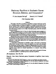
Here player 1 chooses rows and player 2 chooses columns. Not ice that player 2 has nc) influence on the play at all, as he has only one action in both states. In each entry, the corresponding payoff is placed in the upleft corner, while the transition is placed in the bottom-
where rm is as above.
The ~-discounted
value and ~-
discounted optimality
are defined as for limiting aver-
age rewards, and in [5] the ~-discounted value up and stat ionar y /?-discounted optimal strategies are shown to exist.
right corner. In this game each transition is represented by the number of the state to which transition occur with probability
ing, i.e,, if the play visits state 2 then it stays there forever. since player 1 has only one action in state 2, strategies for player 1 only need to be defined in state 1. Consider the Markov tion B with probability
In zero-sum games the players have completely opposite interests, so it is natural to evaluate a strategy fl of player 1 by the reward ~(fi) it guarantees against any strategy of the opponent, For a strategy T let
Using this evaluation relation
“s-better”
@ we may naturally
between strategies
Clearly, ~ yields reward 1/2, hence we obtain
41(~) = 1/2. However, if h* denot~ the history UP to stage 1 when player 1 chooses action T at stage 1, then the strategy ~ [h”] prescribes action T for each stage, hence ~l(~[h”]) = 1. Thus @l (~) < ~l(~[h”]), which means that ~ is improving.
define the
of player 1.
strategies will be simply called better.
1/2 and ac-
1/2 at stage 1, and if the play
does not absorb then to play action T at all further stages.
A 3 Results
strategy # is called e-better than n2, where s 2 0, if ~~ (T1) ~ ~~ (m2) — s holds for all s ~ S. O-better strategy K non-improving
strategy ~ for player 1 which
prescribes to play action T with probability
2 Preliminaries
should
1, Notice that state 2 is absorb-
We will call a
if for any state s E S and for
In this paper the main result is given in theorem
5,
which, verbally and less detailed, can be presented as:
any history h with final state s we have
otherwise
T is called
improving
strategy, for any stat e, cannot guarantee a
improving.
larger reward conditional tially,
Intuitively,
a non-
Main Theorem In any zero-sum stochastic game, for any non-improving strategy, there ezists an E-better stationary .strategy, for any E > 0, and there exists a better Markov strategy as well.
on any past history than ini-
On the other hand, improving
strategiw
may
become better during the play than initially.
The
above
improving For example, non-improving
all stationary strategies are clearly strategies, because z = z [h] for any
history h. In the following simple example we show an instance of an improving strategy.
theorem strategies
says,
that,
~surprisingly, non-
are not more effective
than sta-
tionary strategies or Markov strategies, This also means that, instead of using a complex history dependent non-improving strategy, the pli~yer could also use a simple stationary strategy which guarantees at least the same reward up to some arbitrarily small E >0, or he could even achieve t he same reward by employing a Markov strategy. Notice
that
optimal
strategies
are
always
non-
improving, since they guarantee the value and no higher reward can be guaranteed by the definition of
0-7803-4394-8/98 $10.00 (c) 1998 IEEE
2675
Proceedings of the 37th IEEE Conference on Decision & Control • Tampa, Florida USA • December 1998
the value. Using this observation be seen as a generalization
the above result can
of the following
4 Proof
theorem,
which is proved in [2]:
First we introduce some more notaticms. Let n denote a fixed non-improving strategy and let
Theorem 1 In any zero-sum stochastic game, if player 1 has an optimal strategy, then he also has a stationary E-optimal strategy, for any E > 0, and a Markov optimal strategy as well. The above theorem
and the Main Theorem
a :== f#J(7r).
together
have the following corollary. This shows the insufficiency of the class of non-improving strategies as well as the indispensability of improving strategies for achieving s-optimality,
TP02-3 16:40
where PS(%,YS)
for small E >0.
Corollary 2 In a zero-sum stochastic game, if a player has no stationary c-optimal strategies for small E >0, then he neither has optimal strategies and all his E-optimal strategies, with small c >0, are improving.
= ~ G(L) L ,L
For~GXandy
CY
Ys(js)Ps(tl&,
js).
let
A(z, y) :=
(AS(%,YS)).CS -
For all s ~ S let The next example, the Big Match (cf. an illustration for the above corollary.
[I]),
provides
so X* is the set of mixed actions of player 1 in state
Example 2:
s which assure that after transition a,will not decrease in expectation.
R
L
o
T
1
EEa 1
B
Lemma 3 The sets -%., s c S, are nonempty polytopes.
1
1
0
*
*
Proofi
1
The notation
is the same as in example
this example
Let s G S. One can verify that the lin~rity
of A8 in both components 1.
In fact,
is a 3-state game in which states 2 and
3 are absorbing, i.e. once play reaches such a state, play remains there forever. State 2 has a payoff 1 to
implies that the set X8 is
a polytope. Now we- prove that ~, is nonempty by showing that r, G X., where w. dlenotas the mixed action prescribed by m for stage 1 if the initial state is state s. By the definition of @$(T)
player 1 and is reached (with transition probability 1) from state 1 by playing (B, L); state 3 has payoff O for player
1 and is reached from state 1 by playing
“$4(d%&,~sl),
(B, R). For initial state 1, the limiting average value is VI = ~ and player 1 is known to have neither optimal strategies nor stationary E-optimal strategies for small s > 0.
But for any N
E N player
1 can guarantee
hence using improvingness
the
definition
of
a
and
the
non-
of n we have
by playing the following strategy 7rN: for 4— h any history h without absorption, if k(h) denotes the number of stages where player 2 has chosen action R minus the number of stages where player 2 has chosen action L, player 1 has to play the mixed action:
7r~(h) :=
(
1–
(k(h) +lN + 1)2‘(k(h) +lN + 1)2
)
“
Three results can all be found in [I]. Clearly, the latter strategy nN is improving, since for the history h = (1, T, R) we have 7rN [h] = mN+l.
0-7803-4394-8/98 $10.00 (c) 1998 IEEE
2676
Proceedings of the 37th IEEE Conference on Decision & Control • Tampa, Florida USA • December 1998
so the proof is complete.
❑
TP02-3 16:40
By the finiteness of the state and action there exists a countable subset of discount B
If Z is a polytope then Relint (Z) denotes the relative interior of the polytope Z, which is defined as the set of points in Z which can be written as a convex combination of all t he extreme points of Z with only strictly positive coefficients.
C
(O, 1) such that
there are stationary
1 is a limit
~-discounted
point
optimal
spaces, factors
of 2? and strategies
xp G X’ in the restricted game P such that the sets {i. G 1,1Z@~(Z8) > O}, s E S, are independent of ~ G B. In the sequel each time thak we are dealing wit h discount factors, discounted optimal strategies, or with limits when the discount factors converge to 1,
The following
technical lemma is needed later for the
construct ion of a restricted game. Here, on condition that player 1 uses a strategy z ~ Relint (X), we are looking
we will have such a subset of discount factors 1?in mind.
for the largest set S’ of states which can be
made recurrent and the largest sets Y8’, s ~ S’, of mixed actions which keep all the states in S’ recurrent.
Lemma 4 There exist a nonempty S’ S and a nonempty Y’ = x~cst Y:, where Y; c Y8 are polytopes for all s G S’, such that for any z G Relint(X)
Theorem 5 Let n- G II be a non-improving strategy in a zero-sum stochastic game. By using the strategy T, define S’, X’, Y’, and the restricted game l? as above.
c
(a) for any y G Y, ifs E S is recurrent with respect to (z, y) then s G S’ and y. c Y;; (b) for any y G Y with YS G Relint(~’) tor all s G S’, all states s E S’ are recurrent with respect to (Z,y).
Proofi let R(j) to (z, j).
Take an arbitrary z ~ Relint (~). For j ~ J, denote the set of recurrent states with respect Now let
s’:=uj&l R(j).
(a) For any ~ G B, let X@ G X’ be a /3-discounted optimal strategy in the restricted game I?( and let z c Relint(X), Then, for any .s >0, if/3 c l?, T c (O, 1) are suficzently large then the stationary strategy x; E X, given for state s G S by
x;.:=
T.L-up.+ (l-’ z~ {
T). x.
zfs ifs
Es’ Es\s’
‘
is E-better than x in l?. (b) Let en, n E N, be an arbitrary monotonously decreasing sequence converging to O. Let the stationary strategy xn c X’ be Em-better than n for all n ~ N. Then there exists a sequence Kfi in II such that the Markov strategy jf which prescribes to play xl for the first K1 stages, then to play X2 for the next K2 stages, etc., is better than T.
For s G S’ let
A similar statement holds for player .2 as well. Y; := conv {J~} ,
Y’ :=
X.CSI
y:,
where conv stands for the convex hull of a set. Note that these sets are independent of the choice of z G Relint (X),
because all z & Relint (X)
To illustrate this theorem we present the following example in which we focus on optimal strat gies as non-improving
strategies.
put positive
probability ies on the same actions in any state. It is not hard to check that S’ and Y’ satisfy the required properties. ❑
Example 3: R
L
Recall that we have fixed a non-improving strategy n for player 1. Let X be as above, let S’ and Y’ be as in lemma 4, and let X’ := x S=S X$. In view of lemma 4, we may define a restricted stochastic game r’ in the following way. Let I“ be the game, derived from 17,where the state space is S’ and the players are restricted to use strategim that only prescribe mixed actions in X: and Y: if the play is in any state s G S’. Clearly, X’ and Y’ are respective stationary strategy
The value for the only non-trivial initial state 1 k vl = 1. It is not hard to show that there are optimal
spaces in I“ for the players.
strategies for player 1 (later we will construct optimal
0-7803-4394-8/98 $10.00 (c) 1998 IEEE
1
2677
Proceedings of the 37th IEEE Conference on Decision & Control • Tampa, Florida USA • December 1998
Markov strategies).
Therefore
we have S’ = S for this
TP02-3 16:40
understood to be taken for a sequence of ~’s).
Also, let
game. Following the construction for stationary s-optimal strategies, we have X’ = X, Y’ = {(1, O)}. Now the unique /3-discounted optimal strategy of player 1 in 1? is Zp = (O, 1) for all ~ ~ (O, 1). The role of Z~ is to play well as long as player 2 plays in the restricted game I“, namely to guarantee the value v as long as player 2 chooses action L in state 1. However, an enforcement is needed to make sure that player 2 is not better off by playing Therefore
outside Y’,
namely by choosing. action R.
we take a strategy
z ● Relint (X),
~:={cr~qa.(h)
GY;
for all s G S’ and h G H’};
so ~ and ~ are the set of strategies in the original game r with the property
that, as long as the play is in the
restricted game I“, they behave as strategies in II’ and z’. By using the definition
of ~,
the following
lemma is
straightforward.
for ex-
ample z = (1/2, 1/2), which will force player 2 not to choose action R, since then R leads to absorption with payoff 2. Now for -r,~ ~ (O, 1) we have zj=T.
zp+(l–
T). z=(l/2–
Lemma 6 Let x G X and y G Y. Suppose E is an ergodic set with respect to (x, y). Z5en as = at for all s,t CE,
T/2,1 /2+ T/2). Next,
The strategy Z$ is e-optimal as the stationary
strategies
for large -r and ~ indeed, (p, 1 —p) are e-optimal
we show an important
prop,erty
of the sets
x:,Y;,s E s’.
for
all p G (0, s]. Note that player 1 has no stationary
optimal strategy
in this game. One can argue as follows. If a stationary strategy x prescribes action T with a positive probability then z only gives a reward strictly less then 1 if player 2 always chooses action L.
On the other hand,
if z chooses action B with probability y 1, then if player 2 always takes action R then the reward is O. Thus no stationary strategy can guarantee v = 1.
en = l/n and take the stationary zn = (sn, l — cm) G X’
Proofi
Take a~bitrary s G S’,
Let 2 G Relint (X)
Formally, let
en-optimal
strategy
z. c
X:,
YS) =
and y. 6 Y;.
and y G Y with yt ~ Relint (Y;)
all t G S’. In view of lemma 4-(b), state s belon~
for
to an
ergodic set E with regard to (2, ~), hence by lemma 6, we obtain at = a~ for all t, w ~ E. As p.(tf%, implies t G E, we
A Markov optimal strategy can be constructed as above. The idea is to increase ~ and -r simultaneously during the play so that player 1 plays better and better in the restricted game. However, 7- must be increased sufficiently slowly so that player 2 cannot choose action R “too often” wit bout absorption.
Lemma 7 For any s c S’, we have that A,(x,, a, for all XS ~ X; and y, G Y.’.
y,) >0
must have p~(t]zs, y$) > 0 also
implies t G E, which completes the proof.
❑
Lemma 8 Let s E S’ be an arbitrary initial state and let H, be the set of histories starting in s. Also, let Us := {(h, t) E Hs x S[ P.=a (h) >0
and
for all n e N. Let Km = 1 for
all n c N. Let ~ be the Markov strategy as in theorem 5. So at stage n, the strategy probability
~ chooses action T with
I/n and action B with probability
1 – l/n.
One can verify that f is optimal. VVe only give an intuitive argument. If player 2 chooses action R with a “positive frequency” then absorption occurs with
where P*=V(t Ih) is the probability that, with respect to (z, CJ), the new state becomes state t after history h. Then xt(h) c X; for all (h, t) G U8.
probability y 1 due to the slowly decreasing probabilities
Proofi
on action ~ while almost always choosing action L yields reward 1 since the probabilities on action B
shortest history
state t such that P~To (in)
converge to 1.
some a c ~ and fit (fin) @ Xi.
Suppose the opposite,
Then there exists a
&n c Ha, say up to stage n, and a >0
and ~P~=o (tlfin) >0 Since mt(in)
for
@ X; there
exists a ~t ~ Yt such that We now provide
a proof for theorem
5.
Recall that
we have fixed a non-improving strategy T. In the restricted game r’, let H’ denote the set of finite histories, III and Z’ the sets of history dependent strategies, y’ the limiting avarage reward, vi the f7-discounted value for all @ G (O, 1). Let v’ := ~impTl vj
(here “limit”
0-7803-4394-8/98 $10.00 (c) 1998 IEEE
is
For any present state z t S’ and past history h e H’, we define a mixed action &(h) G Yz as follows: if ~Z (h) c X: then let &Z(h) G Y;; while if m. (h) G xx \
2678
Proceedings of the 37th IEEE Conference on Decision & Control • Tampa, Florida USA • December 1998
X: then let ~Z(h) & YZ such that Az(Tz(h),
&z(h)) < az.
TP02-3 16:40
Lemma 9 We have
By lemma 7, we have in both cases that AZ(~.(h),
C.(h))
< a.-
Proof of theorem 5: By usingthe above lemmas, the proof is almost the same as the proof of theorem 1 in
Let 6 e (o, Psfla(fin)
“ Tsmo(tlin)
oT) .
[2]. Note that lemma 4-(a) is needed for achieving the following crucial property: if a pure stationary strategy
Let S1 := s, and let sm , m ~ 2, denote the random
j c J is a best reply to some x;, then, in any ergodic
variable for the state at stage m, and let 8m denote
set with respect to (xL, j ), the play is in fact taking
random variable for the history up to stage m ~ N.
place in the restricted game I“. ❑
Let IS8 c Z be the strategy that prescribes to play as follows: if Q%= or Sn+l finally,
play u during the first n stages; at stage n + 1, hn and Sn+l = t then play yt while if On # ~m # t then play the mixed action ~~.+, (On); and play a &best reply against fl[@n+l] from stage
n -t 2 on. Note that P.in.8
(fin)
=
P.lfla(ir)
5 References [11 D. Blackwell & T.S. Ferguson [19681: “The big rnatcp, Annals of Mathematical Statkcs- 33, 159-163:
[2] J. Flesch, F. Thuijsman,
>0.
O.J. Vrieze
[1998]: “Sim-
plifying optimal strategies in stochastic games”, SIAM Journal on Control and Optimization 36, 1331-1347. Since we have chosen a shortest history &n with the above property, the play up to stage n has been going in the restricted game l?. By lema 4(b), we must have Sn ~ S’, and by the definitions of X’ and Y’, we obtain in expectation
[3] D. Gillette [1957]: “Stochastic games with zero stop probabilities” , In: M. Dresher, A. W. Tucker&P. Wolfe (eds.), Contributions to the Theory of Games III, Annals of Mathematical Studies 39, Princeton
University
Press, 179-187.
:$lna$ (a,m+l ) = a~,. The choices of the used mixed actions at stage n + 1
[4] J,F, Mertens
imply
games”, International Journal of Game Theory 10, 53-
& A.
Neyman
[1’981]: “Stochastic
66. t~,fic, (a~~+2)
~
f.lna,
(a~m+l) –
P.lmaa(lv)
- P.lma(tp)
.
‘i-.
Since from stage n+ 2 player 2 plays a &best reply and T is non-improving, the choice of 6 yields
‘y,, (7r, d)