Geosci. Model Dev., 3, 189–203, 2010 www.geosci-model-dev.net/3/189/2010/ © Author(s) 2010. This work is distributed under the Creative Commons Attribution 3.0 License.
Geoscientific Model Development
Tracers and traceability: implementing the cirrus parameterisation from LACM in the TOMCAT/SLIMCAT chemistry transport model as an example of the application of quality assurance to legacy models A. M. Horseman1 , A. R. MacKenzie1 , and M. P. Chipperfield2 1 Lancaster 2 School
Environment Centre, Lancaster University, Lancaster, UK of Earth and Environment, University of Leeds, Leeds, UK
Received: 26 October 2009 – Published in Geosci. Model Dev. Discuss.: 17 November 2009 Revised: 19 February 2010 – Accepted: 2 March 2010 – Published: 16 March 2010
Abstract. A new modelling tool for the investigation of large-scale behaviour of cirrus clouds has been developed. This combines two existing models, the TOMCAT/SLIMCAT chemistry transport model (nupdate library version 0.80, script mpc346 l) and cirrus parameterisation of Ren and MacKenzie (LACM implementation not versioned). The development process employed a subset of best-practice software engineering and quality assurance processes, selected to be viable for small-scale projects whilst maintaining the same traceability objectives. The application of the software engineering and quality control processes during the development has been shown to be not a great overhead, and their use has been of benefit to the developers as well as the end users of the results. We provide a step-by-step guide to the implementation of traceability tailored to the production of geo-scientific research software, as distinct from commercial and operational software. Our recommendations include: maintaining a living “requirements list”; explicit consideration of unit, integration and acceptance testing; and automated revision/configuration control, including control of analysis tool scripts and programs. Initial testing of the resulting model against satellite and in-situ measurements has been promising. The model produces representative results for both spatial distribution of the frequency of occurrence of cirrus ice, and the drying of air as it moves across the tropical tropopause. The model is now ready for more rigorous quantitative testing, but will require the addition of a vertical wind velocity downscaling scheme to better represent extra-tropical continental cirrus.
Correspondence to: A. M. Horseman (
[email protected])
1
Introduction
Ice clouds, particularly those categorised as cirrus, have a significant effect on climate and weather processes (Liou, 1986; Lynch, 1996, 2002). Cirrus ice clouds have both a cooling effect, by reflecting incoming short-wave radiation, and a warming effect, by the absorption/re-emission of infrared terrestrial radiation. The radiative balance of the cloud depends on their location and extent as well as the number, size and shape of the ice crystals of which they are composed (Zhang et al., 1999). Cirrus clouds also affect atmospheric chemistry by redistributing water and other compounds in the atmosphere (Robinson, 1980), for example ice clouds are implicated in the regulation of the transport of water from the upper troposphere into the stratosphere (Jensen et al., 1996; Sherwood and Dessler, 2000; Santacesaria et al., 2003; Luo et al., 2003; MacKenzie et al., 2006). Ice clouds are a ubiquitous weather feature with considerable variability, both temporally and spatially, but the occurrence and properties of cirrus are not well captured by current global climate and chemistry models; typically represented by simple saturation adjustment schemes, e.g. the CAM-Oslo model (Storelvmo et al., 2008) and the ECMWF Integrated Forecast System (Thompson et al., 2007). Two different parameterisations of the homogeneous formation of cloud ice have been experimentally added to global climate models (GCMs). The parameterisation of K¨archer and Lohmann (2002a,b) has been incorporated into the ECHAM5 GCM (Lohmann and K¨archer, 2002; Lohmann et al., 2008), and the parameterisation of Liu and Penner (2005) has been incorporated into the NCAR Community Atmospheric Model Version 3 (CAM3) (Liu et al., 2007). Most recently Spichtinger and Gierens (2009) tested their own bulk ice microphysics scheme the EULAG research model for geophysical flows.
Published by Copernicus Publications on behalf of the European Geosciences Union.
190 At Lancaster, we have developed a strategy for modelling cirrus that incorporates recent advances in the theory of homogeneous ice particle formation in a computationally efficient parameterisation (Ren and MacKenzie, 2005). The parameterisation has been used in a Lagrangian model (LACM) that was able to reproduce total water and relative humidity observations in the tropical tropopause layer (TTL) (Ren et al., 2007). We have now integrated this parametrisation into a chemistry-transport model (CTM) to examine the effects of ice on the global water budget, chemistry and radiative transfer. The formation of cirrus ice is especially sensitive to cooling driven by vertical motion, so, by integrating a cirrus parameterisation into an offline CTM that uses wind forcing data from meteorological analyses, we avoid the extra complexity of synthesizing atmospheric dynamics. The same analyses can provide realistic water vapour boundary conditions, allowing us to examine the effect of ice cloud formation on the drying of air entering the stratosphere. In carrying out the model development we have adopted formal software management practice and, in this paper, we use the example of adding a cirrus module to a CTM to draw out general conclusions on developing academic software that maximises its durability and usability. The benefits of formal software management schemes have been proven in pure software projects, but they are often viewed as excessive for individuals and smaller groups of non-software specialists. Consequently, many environmental models still have no or minimal software engineering procedures and quality assurance (QA). Risbey et al. (1996) called for the application of QA in the development of Integrated Assessment models for climate change, and Jakeman et al. (2006) proposed a 10-step development process for model design; but here we extend the discussion to existing software. The two software models involved in this work have been developed over a number of years with limited formal quality control so. As one of us (AMH) has practical experience of software engineering under a quality assurance regime, we also describe the application of a pragmatic process for so-called legacy models. Although they are separate processes, for simplicity we refer to software engineering and QA aspects collectively as software quality control (SQC) in the rest of the text.
2
The rationale for software engineering and quality assurance
Formal software engineering methods and associated quality assurance regimes originated in 1960s as a result of what was dubbed the “software crisis”; too many projects overran both in time and budget. As a direct result, design lifecycle and formal methods were developed, aimed at controlling concurrent development of larger projects by multiple developers, i.e. projects of a size similar to the “community” geoscience models. Advances in the power of deskGeosci. Model Dev., 3, 189–203, 2010
A. M. Horseman et al.: Tracers and traceability top computers, coupled with the reuse of a growing pool of large legacy models, means it is becoming easy to produce models of great complexity (Crout et al., 2009; Nof, 2008). This now gives the individual developer many of the same software management problems that faced collaborative development teams a few years ago. Most obviously, simple software errors can have far-reaching consequences. For example, in a paper based upon statistical analyses using purpose-written software (Krug et al., 1998), a programming error caused double-accounting of some results; the authors had to issue a complete retraction (Krug et al., 1999). Similar examples are the corrigendum by Timmerman and Losch (2005) to ocean modelling work by Timmerman and Beckmann (2004), and the correction of Lohmann et al. (1999b) to Lohmann et al. (1999a) also the result of coding errors. In the first two cases, in the interval between publication of the original work and the correction, the papers had been cited by others. In other cases corrections may be made in the course of other enhancements and reported in papers ostensibly focused on new results, e.g. Yu et al. (2002). There are many reasons for SQC being given a low priority in a particular project: the authors never intended their models to be long-lived, but they have been expanded beyond the original requirements; the model originated before the widespread use of formal methods, or, simply, the author had no interest in SQC. In stark contrast to commercial/industrial software development, scientific software is not always commissioned directly: it is often developed as a means to reach some specified scientific objectives. While the scientific results of a study may be audited (at least by peer-review), the software itself is not. Despite this apparent omission many models have become well respected based upon their results at least by peer-review and, often, by modelling intercomparison exercises. 2.1
Software quality control process
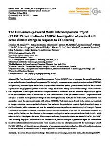
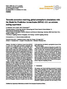
In projects where formal design and SQC are employed from the outset, a project’s life-cycle, processes, procedures and design methodologies would typically depend on its size, which in turn is determined by a scoring system based on factors such as number of requirements, number of developers, type of deliverable, etc. For individuals in a research environment this is difficult to assess at the start, and in the case of legacy models much of this decision making is irretrievable. A representative life-cycle for software development is the waterfall model illustrated in Fig. 1. Each stage of the process depends on the output of the previous one and usually demands extensive documentation, uses specific methodologies (e.g. Structured Systems Analysis and Design Methodology, SSADM, or the European Space Agency’s Hierarchical Object Oriented Design, HOOD, etc.), and language (e.g. Unified Modelling Language), and is controlled by purpose-written procedures and work instructions. This is www.geosci-model-dev.net/3/189/2010/
A. M. Horseman et al.: Tracers and traceability impractical for smaller scale projects by non-specialists. The bulk of the work, and hence SQC overhead, occurs in the stages in the bottom two layers of the waterfall (architectural and detailed design documentation and the corresponding unit and integration testing documentation). These are also the most difficult stages to apply retrospectively to legacy models as most of the work they would describe has already been done. 2.2
191 Start
End User
Validation
Software
Verification Acceptance Testing
Requirements
Architectural
Integration
Key points of SQC Detailed
The objective of any SQC system is to ensure that the end product does what the user wanted in the way the user intended. The purpose of most the SQC documentation is to show external auditors, and ultimately the customer, what has been done. It also simplifies the division of work to teams of specialist programmers who may have little knowledge of the project as a whole; however, in our case, the developers are also the customers and have detailed knowledge of the project. The core of the SQC process is traceability; in the context of a geoscience model from a statement of purpose and mathematical equation to presentation of results. The traceability in the example waterfall life-cycle (Fig. 1) can be broken down into three principal components: requirements, testing and configuration control. When working with legacy models it is not practical to recover the formal design documentation and bypassing these stages saves a great deal of effort without necessarily breaking traceability. However, is still possible to perform testing on the integration of component models, and this can be simply recorded for current and future users and developers. To further reduce the work overhead and scope for human error, whilst still maintaining the core objectives of SQC, we automated as many aspects of the principal development components as possible. The methods we used to achieve this are outlined in the Appendix A, but are obviously not the only possibilities. 2.2.1
Traceability component 1: requirements
This is perhaps the most difficult of the three key components to easily control. The user requirements, and software requirements derived from them, are the starting point of the SQC audit trail and can use documentation in a specialised language. We simplified this by amalgamating the user and software requirements into a hierarchical numbered list starting with the purposes to which the end product is to be put. The list describes one requirement per line/paragraph in plain language using the words “must” and “shall” to indicate mandatory features, and “may” and “should” to indicate desirable but optional ones. This list is the basis for development decisions regarding the equations and references to be used to construct algorithms, and also forms an outline document of the completed software’s features and functions. Setting specific requirements at the outset has the benefit of focusing the subsequent development process. www.geosci-model-dev.net/3/189/2010/
Unit
Design
Testing
Fig. 1. Illustration of a typical “waterfall” type of software lifecycle. The work-flow is through the stages down the left side and back up the right side. The horizontal arrows indicate interdependencies between stages, e.g. the integration tests are designed demonstrate that each architectural design feature has been implemented correctly.
An example project often used to illustrate the application of SQC, in computer science terms, is the implementation of a bank ATM (e.g., Windle and Abreo, 2002). This is popular because the project has a purpose and outputs that can be clearly and precisely defined at the outset. This is rarely the case in a geoscience context, and it is likely that the requirements will be changed in the light of knowledge gained during the development process. This is termed “requirements creep” (see glossary in Appendix A) and is often cited as a major problem for software projects (e.g., Jones, 1996), but as the author points out, there is no definitive cure for it. In academic software, some “requirements creep” may actually be desirable, provided it does not prevent the initial objectives being achieved. Our strategy, adapted from so called “agile” development methods (see Huo et al., 2004 for a discussion of their use in a QA system), was to accept that requirements creep is inevitable and to consider the requirements list a living document. New algorithms/equations and output must be documented in some manner and may well end up in a published paper, but for the development process we chose to simply document these changes as extensive comments in the code at the point of use. This is a practical solution for a scientific project as, unlike in most other types of development, the users are likely to view the source code. It is also probably the most easily adopted method, but is the least automatable stage and relies on the programmer buying-in to the SQC culture at the very point where s/he is struggling with other issues, such as translating the user requirements into code. 2.2.2
Traceability component 2: testing
The waterfall life-cycle example shown in Fig. 1 divides testing into stages: unit, integration and acceptance testing. As might be expected, unit testing exercises individual program Geosci. Model Dev., 3, 189–203, 2010
192
A. M. Horseman et al.: Tracers and traceability
units (the definition of a unit is inevitably imprecise but is usually easy to see in practice) using a “harness” that emulates the interface to that unit, and testing for things like out-of-bounds inputs. Integration testing builds the final program unit by unit with “code stubs” replacing those yet to be added, the objectives being, for example, to test program stability by theoretically running all possible paths through the software. Acceptance testing is intended to determine if all of the requirements have been met, and can be sub-divided into verification and validation. In non-SQC development, testing is centred around the validation of results, ideally against measurements, but often simply against other models; overlooking the verification, integration and unit testing stages. The purpose of verification testing is not to show the results are representative of the real world, but more fundamentally that the algorithms used are the correct implementation of the intended equations. This is of benefit when comparing models of similar purpose as it is inevitable that some will employ similar algorithms as dictated by current understanding of the relevant chemistry and physics, but may still have subtle but significant differences (e.g., Bouzereau et al., 2007). Consequently it is important to be sure which equations are being used for each model, and as models may have different algorithmic implementations, to be aware how they behave. Larger legacy models like our CTM have already undergone integration and cannot readily be sub-divided, so unit testing is impractical. To achieve some form of control at the first stage of testing we used the unmodified first revision of the CTM as a baseline for subsequent regression tests. Unit testing could be performed on the cirrus parameterisation that we have added. In our case, the inputs and outputs to the parameterisation are such that this unit test could also be considered a component verification test. We used a sensitivity analysis of the parameter space, the details of which are described later in Sect. 4.2. Integration testing was also possible for our example, but as there is only a single connection point and a great difference in size between two components, it was simpler to merge the integration and validation stages. 2.2.3
Traceability component 3: revision/configuration control
Arguably this is the most important aspect of maintaining traceability; it is also the easiest process to automate. It involves recording sets of changes to all the components of a model development including documentation, code, inputs and results, and applies throughout the development process not just at major release points. There are many tools available for control of program files, many are cross-platform using a local, client-server or distributed approach, and many are free of charge. Examples are SCCS, BitKeeper, Subversion, CVS, Git, etc.; we chose Subversion as its use of a central repository with network access for multiple users fitted Geosci. Model Dev., 3, 189–203, 2010
our development process. We used a fine-scale incremental approach to control, so that as each set of changes with an identifiable outcome was completed it was “committed” to the revision control system. This allows the point at which specific changes were made to be identified, and if necessary, undone. The use of a software tool to track changes also simplifies code branching and merging, where, for example, alternative algorithms can be tried out and the best incorporated into subsequent development. All code, and, where practical, data files, were “checked-in” to this tool. We also use Subversion to manage multiple code trees and ancillary text files noting aspects of the models discovered during development. A less obvious aspect of traceability is the control of the analysis of results. It is standard scientific practice to record how, and from where, analysis outputs were obtained. With modern analysis tools – such as MATLABr , IDLr , PV WAVEr and CDAT – the software development of a project does not stop at the data files produced by the model. To be able to trace an output figure back its algorithmic basis the analysis tool scripts and programs need to be controlled as well. We considered analysis programs to be part of the code-base and so added them to the repository.
3
The model build process: SLIMCAT-cirrus
When working with legacy models, any SQC scheme used must adapt to the current state of those models. The CTM used is TOMCAT/SLIMCAT (Chipperfield, 2006) a well proven and widely used model e.g. Feng et al. (2005), Kilbane-Dawe et al. (2001) (see http://www.see.leeds.ac.uk/ slimcat for a more comprehensive list of publications). It is an offline model, i.e. it does not perform full atmospheric dynamics calculation, but uses temperature, pressure, humidity and wind forcing data, primarily from the ECMWF operational analysis and re-analysis. Vertical wind velocity is not taken directly from the re-analyses for the reasons described in Weaver et al. (1993). Instead, the transport functions of the model employ the advection scheme of Prather (1986) driven by a vertical flux determined from the adiabatic heating rate. The ERA-40 reanalysis data (Uppala et al., 2005) was used in most of the development work although the modified SLIMCAT retains the original version’s capability of using data from a number of different sources. The cirrus parameterisation implementation used is based upon that of K¨archer and Lohmann (2002a,b) and Ren and MacKenzie (2005). Its use within a domain-filling Lagrangian framework (LACM) is described in Ren et al. (2007). In this work, we adapted the parameterisation for use in an Eulerian framework. This adaptation is practical because the core of cirrus parameterisation is effectively a zerodimensional scheme that describes the evolution of the ice at a single point. Its algorithms only require the ambient pressure, temperature, amount of water vapour and pre-existing www.geosci-model-dev.net/3/189/2010/
A. M. Horseman et al.: Tracers and traceability ice, and vertical velocity at that point. The formation of ice is represented in two stages, initial nucleation and a subsequent growth process. To complete the ice life-cycle, a removal scheme is needed. The existing implementation adopted uses a sedimentation scheme adapted from Pruppacher and Klett (1998) to give a mechanism for moving ice vertically. The parameterisation growth process is bi-directional so it automatically represents evaporation where atmospheric conditions dictate. 3.1
Model requirements
The requirements list used for the development can be summarised as follows: – at each CTM time-step the model must provide the number of ice crystals and ice mixing ratio in each CTM grid, – the number of ice crystals and ice mixing ratio should be made consistent by assuming crystals are spherical with a single size mode and mean radius, – the representation of ice must include a scheme to represent the transfer of ice, from each grid cell to those below it, by sedimentation, – the sedimentation scheme may assume that the ice can only travel to the model grid cell immediately below in one model time step and that the removal process is purely vertical. In addition to these were specific implementation requirements, for example: – the implementation of the parameterisation should be portable, i.e. it may be used with other host models with minimal modification, – the implementation of the parameterisation must be usable, without any modification, with a separate harness for testing purposes. As the structure of the host is far more complicated any modification to it has a greater risk of unexpected side-effects therefore another desirable requirement is that: – modification of the host model should be kept to a minimum. The inputs to the parameterisation described in Ren and MacKenzie (2005) place a software requirement on the CTM i.e. the host model must provide values for temperature, pressure, amount of water, aerosol number and size, and vertical velocity for each grid cell. The sedimentation scheme adds the vertical extent of the grid cell to the requirements of the CTM output. Prior to modification SLIMCAT used the values from the meteorological analyses to represent the www.geosci-model-dev.net/3/189/2010/
193 amount of water vapour in the tropical troposphere (originally defined as the the area where both potential temperature is ≤380 K and potential vorticity is ≤2 PVU). Using the cirrus parameterisation to control water vapour at the top of the troposphere would conflict with the values for water vapour that the CTM takes from the ERA-40 re-analysis files. Consequently it was necessary to modify the limits of the zones in which ERA-40 humidity values are used. Reanalysis data is now used in the region below the 340 K isentrope in the tropical troposphere (defined as where potential vorticity ≤2 PVU); and below 300 K otherwise. The CTM advection process transports water vapour to areas outside these regions and the parameterisation regulates the amount of water entering the stratosphere. 3.2
Modification of the CTM and parameterisation implementation
As the scale of the project would normally determine the SQC procedures taken, a retrospective project scaling determines what remedial work was practicable for the two legacy models. SLIMCAT has a long history of development: it has acquired a large code base from a number of contributors and as consequence would be considered a large-scale project. The cirrus parameterisation is a far smaller development, with one principal developer, and one main objective, which means that it can be considered a small-scale project at its outset. 3.2.1
Preparatory rework
The version of TOMCAT/SLIMCAT used (unicat0.80) comprises a library of upwards of 50 000 lines of FORTRAN77 code that is used with the Cray “nupdate” utility to produce a number of different variants of the model for different purposes. This means that it is far too large for extensive reworking, so a baseline and regression approach was used, a stratospheric chemistry variant of the model (produced by script mpc346 l i.e. based upon run 346) was chosen. A replacement for “nupdate” was written in Perl and used to produce modular source code files from the existing library. The modular SLIMCAT can then be used in conjunction with the ubiquitous GNU “make” utility, aiding portability and speeding up the development cycle. Once the reworked code passed initial testing it was “baselined” in Subversion and further modifications controlled. The large number of published papers describing work done with SLIMCAT serves both as basic algorithm documentation and validation of the baseline. The cirrus parameterisation is a small-scale project, so retrospective application of some SQC was practical. This comprised a complete code-walkthrough and refactoring (see the glossary in the appendix). The main tasks were the application of a coding standard, some modularisation, attribution of each algorithm to a literature source and updating of Geosci. Model Dev., 3, 189–203, 2010
194
A. M. Horseman et al.: Tracers and traceability
comments to reflect this, and bug fixing. During this process the parameterisation was reconfigured to be used as a separate library function so that the same executable code that is used with the CTM can be exercised using an external test harness thus meeting one of the requirements. 3.3
Integration of component models
The CTM is already a time-stepping model and the parameterisation, in its simplest form, is a single-shot representation. Consequently, the CTM host model controls time. As it was the intention to minimise the modifications to the CTM, the link between the CTM and the cirrus parameterisation was limited to a single calling-point. An interface layer was built at this point so that the parameterisation library could meet a portability requirement by adapting the interface and not the library. The interface is the only new code module that needs any knowledge of the host CTM’s data structures and performs a two-way translation of structure and units as well as managing the effects of cirrus ice formation/evaporation on the CTM’s water vapour tracer (a tracer is a passively advected atmospheric component). To minimise the modification of the CTM’s output system, a separate, reconfigurable, output file system was attached to the interface layer. Again this can be reused alongside the parameterisation in other host models with minimal modification and produces self-documenting NetCDF files (http: //www.unidata.ucar.edu/software/netcdf/) to simplify analysis traceability. It was inevitable that some modifications would have to be made to the CTM, mainly to accommodate two new tracers to represent ice in the CTM’s flexible tracer scheme. These quantify the ice formed by the parameterisation as the equivalent volume mixing ratio of water vapour, and the ice crystal number concentration. Once added, these tracers are automatically incorporated into the CTM transport scheme. The mean ice crystal radius (a requirement) can be recovered at each time step by assuming a single mode mean crystal radius (crystals are assumed to be spherical as it is not currently practical to incorporate a full micro-physical model and calculate the wide variety of ice crystal size modes and shapes). 3.4
Data management
The flexible output configuration system allows a number of the model’s internal tracer values to be extracted, spreading the output over a number of files to reduce the size of individual files for analysis. However this does complicate the management of traceability, consequently runs of the model are “wrapped” using a UNIXr /Linuxr shell script that automatically time-stamps the output. The script also collates information about the current revision of the model, inputs and configuration that produced the output, greatly simplifying the logging of the iterative unit/integration test process. Geosci. Model Dev., 3, 189–203, 2010
To prevent any confusion between output files with the same name, each output file has a unique checksum associated with it that is carried through subsequent processing via NetCDF file variables to a status label on output figures. Unfortunately space does not permit them to be legibly reproduced in the all figures shown here. The principal analysis was done with the Climate Data Analysis Tool (CDAT) tool (http://www2-pcmdi.llnl.gov/cdat) – which is based on the object-orientated Python language – and Gnuplot. To be able to track the processing that was performed within the analysis each method or script applied to the data was written to automatically update either the status label or plot title, e.g., the file id in Fig. 2.
4 4.1
Testing and results Unit and integration testing
Most of the details of the unit and integration details are not worth describing here, it is sufficient to state that the end result of these stages was a stable program that produces the outputs needed for verification and validation. The unit testing of the parameterisation covered, for example, the effects of running the nucleation and growth process with and without the sedimentation. Alternative methods of calculating the saturated vapour pressure over ice – i.e. the methods of Marti and Mauersberger (1993) vs. the more recent Murphy and Koop (2005) – showed that the differences did not have a significant effect on resulting ice. Testing the sedimentation scheme on its own showed a discontinuity in the relationship between the ice crystal size and its terminal velocity at around 1 mm radius. This was traced to the use of Beard’s empirical fit (p. 417, Pruppacher and Klett, 1998) outside of its range of validity within the method to calculate the ice crystal Reynold’s number, and required the application of a work around. 4.2
Verification
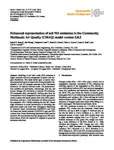
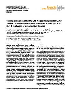
Since the parameterisation was deliberately developed as a library, it can be run with a test harness for sensitivity runs. The driving parameter that has most impact on the production of cirrus ice is the rate of cooling due to vertical ascent (Lin et al., 2002). Figure 2 shows the evolution of the cirrus ice mixing ratio and ice crystal number concentration for a number of different updraft velocities using build 123 of the parameterisation. The details of the build revision numbering system are not relevant, but it is important that a code revision and set of results can be associated. The tic marks shown on the time axis of Fig. 2 are spaced at a typical advection time-step of the CTM i.e. 1 h. It can be seen from the number concentration panel that ice nucleation is effectively instantaneous, and both panels show that the ice growth and removal processes would not be well www.geosci-model-dev.net/3/189/2010/
A. M. Horseman et al.: Tracers and traceability
195
Ice Mixing Ratio (ppmv)
Ice Mixing Ratio Dependence on Updraft Velocity 800 700 600 500 400 300 200 100 0
1 m/s 0.5 m/s 0.2 m/s 0.1 m/s 0.05 m/s
Number Concentration Dependence on Updraft Velocity Crystal No. Conc. (#/m3)
1e+08 1e+07 1e+06 1e+05 1e+04 1e+03 3600
7200
10800
14400
18000
21600
Time (s) File-ID: output-1ms.dat-c523115 output-0.5ms.dat-afd1446 output-0.2ms.dat-c036757 output-0.1ms.dat-3d94cd5 output-0.05ms.dat-ecda739
Fig. 2. Sensitivity of the ice mixing ratio to vertical velocity. This shows the evolution of ice amount as water vapour volume mixing ratio and crystal number concentration derived from the homogeneous nucleation parameterisation. These figures are from the unit testing of the parameterisation separately from the CTM. The initial values of temperature, pressure, etc. are fixed and only the vertical ascent velocity is changed. The time axis tic marks are chosen to show a typical CTM sample rate.
represented at the CTM’s sample rate. To avoid this problem, the cirrus routine splits the CTM time-step into many, smaller, time-steps. During verification the size of the time step was subjectively chosen to sufficiently resolve competion between nucleation, and the increase in relative humidity during ascent and still give a reasonably rapid computation. Figure 3 also demonstrates that the relationship between ice cloud properties and the updraft velocity is not simple. This is most clearly illustrated by the 0.2 m s−1 case, in which there are two nucleation events, whereas there are only single nucleation events for updraft velocities larger or smaller than 0.2 m s−1 . This behaviour comes about because of competition between increasing supersaturation, due to ascent, and decreasing supersaturation due to the growth of existing particles (e.g., Jensen et al., 2007; Lin et al., 2002). As well as making it necessary to step through the cirrus routine in small time increments, this complicated relationship between ice formation and updraft also prompts concerns regarding loss of detail in the upscaling of vertical wind velocities to the comparatively coarse spatial resolution of the CTM. The CTM is typically run at a horizontal grid resolution of ≈2.8◦ , and uses forcing data at T42 spectral truncation. However forcing data is available at higher resolution (up to T799 in the case of operational analyses); this aspect is discussed more fully in Sect. 4.4.1.
www.geosci-model-dev.net/3/189/2010/
4.3
Validation
This section describes the initial stage of the validation process. Its purpose is to demonstrate that the results from the integrated model are not pathological i.e. it does not readily generate unphysical values, and that results can be considered reasonable. A more rigorous quantitative examination of the model will follow in subsequent papers. The ideal reference data for validation would be comprehensive in-situ measurements of the same quantities that are output from the model. Possible sources are balloon and aircraft campaigns which offer high resolution data, but these are narrow in temporal and spatial extent. The model output is large in temporal and spatial extent, but of low resolution. Satellite data is a better match in resolution and coverage, but then comparison is not straightforward because the retrieval of cirrus quantification data is subject to variations in background, similarities to other cloud types, and requires the analysis of radiances scattered or emitted over a wide spectrum (Minnis , 2002). The representation of ice in the model as an ice water volume mixing ratio and crystal number concentration is pertinent to atmospheric chemistry of the requirements, but not readily comparable with the quantities available from satellite retrievals. Stephens and Kummerow (2007) reviewed the methods by which cloud parameters are derived from satellite sensor data, and Zhang et al. (2009) specifically compared the methods used to retrieve cloud products Geosci. Model Dev., 3, 189–203, 2010
196
A. M. Horseman et al.: Tracers and traceability January 1998
January 1999
60 30 0 -30 -60
60 30 0 -30 -60
-120
-60
0
0
10
60
20
120
30
-120
40
50
-60
60
0
60
70
120
80
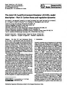
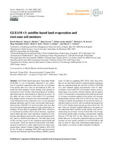
Fig. 3. Comparison of the frequency of occurrence of ice (units are %) between that diagnosed by the model (top row) and values from the International Satellite Cloud Climatology Project (ISCCP) (bottom row). These are both monthly mean values for January 1998 (left column) and 1999 (right column). The model data is for all time samples whereas the ISCCP data is for daytime only with the black areas within the ISCCP plots indicating missing data associated with the polar night. Comparison between model and the ISCCP figures show similar frequencies of occurrence and spatial distribution in the tropics.
from MODIS and POLDER. Both concluded that, as the retrievals are themselves based on models, their uncertainties can be considerable. An example of this is demonstrated by Lohmann et al. (2008) based on the difference between in-situ (MOZAIC) and remote (MLS) sensing observations of relative humidity. This highlights the problem of relying on validation as a method for testing all of a model’s development. To speak colloquially: although “the proof of the pudding is in the eating”, geoscience models are required to provide more than satisfying comparisons with data. Models are required to function as tools for learning about how the observations came about, and SQC can help to ensure that models serve this purpose. 4.4
Ice parameter comparison
We chose the spatial distribution of frequency of occurrence of cirrus as an initial validation quantity because the International Satellite Cloud Climatology Project (ISCCP) has already produced reference climatologies by merging data from multiple sources (Rossow and Schiffer, 1999). The ISGeosci. Model Dev., 3, 189–203, 2010
CCP climatology is not immune to the translation error described above but, by using it primarily as a spatial distribution test, we reduce the susceptibility to quantitative variations arising in processing. However to obtain this quantity from the model output, some post-processing was still required and therefore incorporated into the SQC scheme. First we derived the optical depth (τ ) of cirrus in each grid cell using the method of Stephens (1978) i.e. τ=
3IWPQe 4rρice
(1)
where ρice is the density of ice, r the mean radius of the ice crystals and IWP the ice water path (g m−2 ). Qe is the extinction efficiency, like Meerk¨otter et al. (1999) we treat the ice crystals as spheres with a radius large compared to the wavelength of the incident radiation; hence the extinction efficiency is approximately a constant value of Qe =2 (Petty, 2004). Using optical depth incorporates all the required model ice related output into one test quantity. We then apply a threshold-and-count method to τ to obtain the frequency with which the amount of ice in a grid cell caused www.geosci-model-dev.net/3/189/2010/
A. M. Horseman et al.: Tracers and traceability
197
June 1998
June 1999
60
30
0
-30
-60
60
30
0
-30
-60
-120
-60
0
0
10
60
20
120
30
-120
40
50
-60
60
0
60
70
120
80
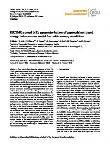
Fig. 4. Similar comparison of the frequency of occurrence of ice to those shown in Fig. 3. Again the top row is frequency of occurrence from the model and the bottom row from the ISCCP. This figure shows mean values for June 1998 (left column) and 1999 (right column). The relatively high values in the model data for the area below approximately 55◦ S are polar stratospheric clouds.
the optical depth to exceed a chosen threshold. The correct value for the threshold is difficult to determine and choosing a lower value would raise the frequency of occurrence values especially in those areas with small amounts of ice. We use a value for τ of 0.01 to include some cirrus classified as subvisual; Sassen and Cho (1992) put an upper limit of 0.03 on the optical depth of sub-visual cirrus. Comparisons between the model (build 125) and ISCCP data are shown in Figs. 3 and 4. Both figures show data show monthly mean values from both ISCCP (top panels) and model (bottom panels); however, the ISCCP data is for daytime cirrus only because of its dependence on visible wavelength passive sensors. The interval between model output samples matches that of the forcing files i.e. at 00:00, 06:00, 12:00, and 18:00 UTC; consequently it is difficult to extract data for only those areas in daylight as different points in the diurnal cirrus cycle are sampled depending on longitude. January 1998 and 1999 (Fig. 3) were chosen specifically so that movements of prominent features of the cirrus fields in the ISCCP data, especially those due to the contrasting El Ni˜no (1998) and La Ni˜na (1999) phenomena, should be clearly visible in the model output. The features include the
www.geosci-model-dev.net/3/189/2010/
different positions of the equatorial western Pacific warm pool in the two years, and the consistent continental convection. The cirrus associated with South Atlantic convergence zone is especially clear in January 1999 and there is evidence of the South Pacific convergence zone in the January 1998 data. It can be seen by comparing the top and bottom panels that the location and shape of these major areas of cirrus in the tropics are reasonably well predicted by the model. Comparison between the January (Fig. 3) and June (Fig. 4) values for both years shows that, again, model and measurement have similar features, most significantly the northward movement of cloud associated with the inter-tropical convergence zone (ITCZ). Other notable features apparent in both are the cloud associated with the summer monsoon over the South China Sea and cloud to the west of Mexico possibly associated with the North American monsoon. The model data for June also shows a large expanse of ice clouds over the Antarctic. These are generally above the tropopause and are polar stratospheric clouds which occur in the model data because the homogeneous nucleation parameterisation does not distinguish between the ice cloud types in the meteorological taxonomy.
Geosci. Model Dev., 3, 189–203, 2010
198 4.4.1
A. M. Horseman et al.: Tracers and traceability Sub-grid scale variations in vertical wind speed
The presence of extra-tropical cirrus is less well represented, especially over the continents, during the boreal summer (Fig. 4). Lynch (2002) provides five types of cirrus formation: synoptic, injection, orographic, cold-trap and contrail. The model resolution is probably sufficient to show the cirrus generated by synoptic and cold-trap mechanisms, but, as can be seen from Fig. 2, the ascent velocity, and hence cooling rate, is critical to the amounts of ice formed. Therefore injection cirrus from continental deep convection may be missing as the model’s horizontal resolution is insufficient to capture the spatially narrow ascent. In fact, the CTM, running at a spatial resolution that makes including a reasonably complete chemistry scheme computationally tractable, does not use all the vertical wind information available in the forcing files. This is because the forcing data are available at greater spatial resolution, and, as mentioned earlier, the values are obtained from the horizontal divergence of the wind field. We are working on a statistical downscaling technique to incorporate as much detail as possible from the existing forcing files, which will be incorporated into the next stage of the work. Even when all the available meteorological data is utilised, there will still be sub-grid scale vertical velocities, For example, Hoyle et al. (2005) and Haag and K¨archer (2004) note that sub-grid scale gravity waves also have a significant impact on ice formation in the absence of convective or orographic influence. This issue is not new; in their work in adding a cirrus parameterisation to GCMs, both Lohmann and K¨archer (2002) and Liu et al. (2007) faced the same problem of sub-grid scale fluctuations in vertical wind speed. The former used the turbulent kinetic energy (TKE) available from the model dynamics scheme to estimate the updraft fluctuations. The authors of the latter noted that they would like to use the same approach, but as the necessary TKE was not available from their host model (CAM3), they resorted to adding a Gaussian distribution with a standard deviation of 25 cm s−1 . TKE is not available in our CTM either, so a different approach is needed. We defer treatment of this scale of process until the issue of capturing all the velocity information in the forcing files has been resolved. 4.5
Water budget testing
The frequency-of-occurrence test (Fig. 3) only exercises the outputs quantifying atmospheric ice. One of our primary scientific requirements was to investigate the amount of water vapour passing through the tropical tropopause layer (TTL). To test this, we need data describing the vertical profile of water vapour in a region that has not been well sampled until comparatively recently (Kley et al., 2000). The SCOUT-O3 campaign over Darwin in November 2005 (Vaughan et al., 2008) provides a suitable data set, with the caveat that the spatial extent of the data is limited as mentioned above.
Geosci. Model Dev., 3, 189–203, 2010
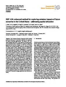
A comparison with model data concentrating on the TTL is shown in Fig. 5. As the measured data come from the aircraft-borne FISH hygrometer (Schiller et al., 2009), they are point values along a flight profile, the model values shown are mean values from November 2005 averaged over the Tropical Warm Pool region. The horizontal bars on the model data trace indicate the spread of the values within the region sampled. For comparison, the diagnosed amounts of water vapour in the ECMWF-Interim reanalysis files used to drive the model are also shown. (Re-)analysis datasets, such as that used here, use data assimilation methods to drive the analysis towards observations. The FISH data have not been assimilated into the ECMWF re-analysis. The remaining trace in the figure shows the amount of water vapour predicted by the model without the cirrus parameterisation i.e. the amounts advected from below the threshold described in Sect. 3.1. It can be seen from this figure that the formation of cirrus ice does remove water at altitude with the minima of both measurements and model results occurring at an altitude of around 16.7 km; the spread of the model results falling within the spread of the measurements. Comparison between values from the model with and without the parameterisation shows that ice formation is reducing the amount of water vapour, bringing the levels present down to that diagnosed by the ECMWF re-analysis in the troposphere, and even lower around the tropopause. 4.5.1
Numerical validation
The next stage of validation within the development process would be to obtain statistical values for the comparisons between modelled and measured data. This could start in the form of correlation diagrams necessitating regridding of the data as preparation for the calculation of a number of metrics for example Pearson’s product-moment correlation coefficient, Spearman rank correlation, coefficient of efficiency, root mean square error and mean absolute error, etc. Willmott (1981), Legates and McCabe (1999) and Wilks (2006) amongst others discuss the techniques and metrics used in evaluating model data. A suite of test metrics is preferable because, as these authors point out, each has at least one limitation. More than one quantity and preferably more than one measurement dataset should be considered the goal to exercise different model components. The initial validation of our model, although simple, has already identified a significant model limitation, so we adjourn the rest of the validation of SLIMCAT-Cirrus until the issue of capturing more sub-grid scale effects has been addressed. In the complete software development scheme the results of the validation steps provide a basis for future regression testing; used to assess improvements, as well as to ensure that changes do not have a detrimental effect on existing performance.
www.geosci-model-dev.net/3/189/2010/
A. M. Horseman et al.: Tracers and traceability
199
H2O vertical profile of mean level averages for November 2005 20 120.0oE to 140.0oE : 0.0oN to −20.0oN SCOUT−O3 FISH data: 19/11/05 SCOUT−O3 FISH data: 25/11/05 SCOUT−O3 FISH data: 23/11/05 Model − No Cirrus ECMWF−Interim Model − Cirrus
19
18
Altitude (km)
17
16
15
14
13
12 1.0e+00
1.0e+01 Water vapour (ppmv)
1.0e+02
File ID: 2ab30e8 ./Nov05_05.nc interp on GeoP_Hgt
Fig. 5. Comparison of vertical profiles of water vapour from the integrated model and measurement data. The grey background points are data gathered by the aircraft-borne FISH instrument during the SCOUT-O3 campaign over Darwin in 2005. The measured data are point samples whereas the model data are the monthly mean of model cells from the region at each height layer. The horizontal bars on the model data show the range of values found on each layer in the region. The magenta trace shows the water vapour values from the model with advection from within the meteorological analysis region, but without the cirrus parameterisation. The ECMWF-Interim trace shows the amounts of water vapour diagnosed in the meteorological analysis.
5
Conclusions and future work
The adoption of the pragmatic SQC scheme described here has not proved to be a significant overhead, but it has streamlined the development process. The resulting audit trail has proven to be useful for controlling model development, and the automation system we produced can be applied to other projects. Our experience of applying basic SQC methods suggests that there should be greater emphasis placed on quality control and software engineering even in informal developments. Indeed, the use of academic “experimental” research software in highly influential policy-facing programmes, such as the IPCC or the WMO-UNEP ozone assessments, make such software less “informal” than may first appear. The system we describe cannot eliminate all errors and oversights, but it does help to detect them, as well as simplifying the identification of the results affected. For our particular model development project, the results presented here are promising: both the amounts of ice formed and water vapour removed appear to be reasonable, especially in the tropics. The next stage of work will be twofold. First, in an effort to better represent extra-tropical continental cirrus, we will develop a downscaling system to incorporate information from the high-resolution forcing files that is lost
www.geosci-model-dev.net/3/189/2010/
in the lower-resolution chemistry-transport runs. Secondly, we will perform a more quantitative evaluation of model performance. The latter will use longer time-scales and will benefit from the availability of higher resolution data from active sensors, specifically the A-train satellite’s CALIOP lidar on CALIPSO. Appendix A Key SQC scheme features The simplest step toward introducing SQC to a project is to employ a coding standard. Formally these would be specified as part of the project management process, but as the end product model is likely to be further developed by others, we made this a requirement. The exact details of the coding standard we adopted are not relevant and there are many readily available on the internet, e.g. http://dbwww. essc.psu.edu/lasdoc/programmer/4fortran.html. Most are designed to help the developer avoid the common pitfalls of programming e.g. proscribing the use of the equality operator with floating point operands, as well as incorporating useful guidance: e.g. prescribing variable and function naming conventions to improve code clarity for both the original Geosci. Model Dev., 3, 189–203, 2010
200
A. M. Horseman et al.: Tracers and traceability
Table A1. Traceability methods – key features. Project Stage/Aspect
Implementation of control
Algorithmic basis
Comment every non trivial line in the code including a reference and if possible text representation of the basis equation. This is prescribed by the coding standard.
Code base control
Subversion revision control system and repository including all source, analysis programs and where possible data. A “commit” is performed after any modifications that passed any informal or formal test.
Build control
The GNU Make utility manages dependencies between files. This allows a faster build cycle, as only those modules that have been changed are rebuilt. Some program switches that change the behaviour of the model that had previously been done by the direct modification of global variables has been centralised using preprocessor directives in the Makefile, making control visible at a single point.
Code modifications (during testing)
At runtime a record of Subversion “status” revision for all source files, and the output of “make -n” to indicate how the executable used differs from the last formal revision is kept with any output.
Input data
As the input files that configure the model for a run are small we used both copying to results repository and revision control. Forcing files must not be changed so are simply held in their own read-only repository.
Runtime
The execution of the model is controlled by a “bash” shell script that encourages the user to identify the purpose of the run and automatically gathers the information from the Build control, Code Modifications, Input and Results stages into a single, time-stamped, results directory. The console output to stdout and stderror during the run is also captured.
Results
Model output is in the form of NetCDF self-documenting files. Checksumming of results files using md5sum command guards against file confusion of similarly named files.
Analysis
This continues the audit trail using a field in the NetCDF output to allow the original file name and checksum to be propagated through post-processed files to analysis using CDAT or GNUplot. The original file checksum is displayed on output plots along with a summary of the processes that have been applied to the data, along with any associated values, e.g. display threshold. This achieved by ensuring that all CDAT methods in the analysis programs apply an annotation to the output title or a status line on each plot. GNUplot is used for simpler 2-D analysis and uses data extracted from the model output via CDAT, which adds a header to the data file listing the data’s origin. All analysis programs are also under revision control.
Table A2. Glossary of terms. Term
Definition
Baselined
Defining a revision of source code deemed sufficiently complete and stable to serve as a point of reference for further development.
Check-in
Add a new item to the revision control system.
Code-stub
A dummy function/subroutine stand-in for more complex function/subroutine yet to be added. Typically the stub will ensure that any return variables from a call have a representative value.
Code-walkthrough
A line-by-line review of project source code, typically performed by an auditor/s other than the code’s authors.
Commit
Create a new revision of an item within the revision control system.
Harness
A piece of source code/data specifically designed to test and monitor all the aspects of a function or subroutine on its own.
Refactoring
Modifying existing code to improve its implementation without changing its external behaviour.
Regression
In this SQC context regression is a set of tests used to demonstrate that successive revisions do not have unexpected side-effects, i.e. any changes in output between revisions can be attributed to the desired effects of modifications
Repository
Location of the revision control systems storage.
Requirements creep
Modification to a project’s requirements after the design stages have begun. Often viewed as a problem as the all the subsequent life-cycle stages are dependant on the requirements, and should therefore be repeated.
Revision
A record of the form of a project file or files at a point in development designated as significant by the project developers i.e. the result of a “commit”.
Revision control
Management of successive changes to project source and document files. A revision control system will allow restoration of, and comparison between, revisions. An important aspect of revision control is that revisions are never removed, only superseded.
Rework
Modifications to existing code that may have already passed through testing to improve the implementation, fix bugs etc., but not necessarily to add features.
Geosci. Model Dev., 3, 189–203, 2010
www.geosci-model-dev.net/3/189/2010/
A. M. Horseman et al.: Tracers and traceability and subsequent developers. Adaptations of general-purpose standards to a geoscience context with the addition of rules such as “all variables must have their purpose and, if applicable, units commented at the point of declaration”, are advantageous. A summary of the other control methods we employed are given in Table A1, and a glossary terms is given in Table A2. Acknowledgements. The authors would like to thank Chuansen Ren for providing and assisting with the use of the cirrus model. The ISCCP D2 data were obtained from the International Satellite Cloud Climatology Project web site http://isccp.giss.nasa.gov maintained by the ISCCP research group at the NASA Goddard Institute for Space Studies, New York, NY in July 2009. This work was partly funded by the SCOUT-O3 Integrated Programme of the European Commission under contract number GOCE-CT-2004505390 and by NERC studentship NER/S/A/2006/14022.
Edited by: V. Grewe
References Bouzereau, E., Musson-Genon, L., and Carissimo, B.: On the Definition of the Cloud Water Content Fluctuations and Its Effects on the Computation of a Second-Order Liquid Water Correlation, J. Atmos. Sci., 64(2), 665 pp., 2007. Chipperfield, M. P.: New version of the TOMCAT/SLIMCAT offline chemical transport model: Intercomparison of stratospheric tracer experiments, Q. J. Roy. Meteor. Soc., 132, 1179 pp., 2006. Crout, N., Tarsitano, D., and Wood, A. T.: Is my model too complex? Evaluating model formulation using model reduction, Environ. Modell. Softw., 24(1), 1–7, 2009. Feng, W., Chipperfield, M. P., Davies, S., Sen, B., Toon, G., Blavier, J. F., Webster, C. R., Volk, C. M., Ulanovsky, A., Ravegnani, F., von der Gathen, P., Jost, H., Richard, E. C., and Claude, H.: Three-dimensional model study of the Arctic ozone loss in 2002/2003 and comparison with 1999/2000 and 2003/2004, Atmos. Chem. Phys., 5, 139–152, 2005, http://www.atmos-chem-phys.net/5/139/2005/. Haag, W. and K¨archer, B.: The impact of aerosols and gravity waves on cirrus clouds at midlatitudes, J. Geophys. Res., 109, D12202, doi:10.1029/2004JD004579, 2004. Hoyle, C. R., Luo, B. P., and Peter, T.: The Origin of High Ice Crystal Number Densities in Cirrus Clouds, J. Atmos. Sci., 62, 2568–2579, 2005. Huo, M., Verner, J., Zhu, L., and Babar, M. A.: Software Quality and Agile Methods, Computer Software and Applications Conference, 2004, COMPSAC 2004, Proceedings of the 28th Annual International, 1, 520–525, 2004. Jakeman, A. J., Letcher, R. A., and Norton, J. P.: Ten iterative steps in development and evaluation of environmental models, Environ. Modell. Softw., 21(5), 602 pp., 2006. Jensen, E. J., Toon, O. B., Pfister, L., and Selkirk, H. B.: Dehydration of the Upper Troposphere and Lower Stratosphere by Subvisible Cirrus Clouds near the Tropical Tropopause, Geophys. Res. Lett., 23(8), 825–828, 1996.
www.geosci-model-dev.net/3/189/2010/
201 Jensen, E. J., Ackerman, A. S., and Smith, J. A.: Can overshooting convection dehydrate the tropical tropopause layer?, J. Geophys. Res., 112, D11209, doi:10.1029/2006JD007943, 2007. Jones, C.: Strategies for managing requirements creep, Computer, 29(6), 92 pp., 1996. K¨archer, B. and Lohmann, U.: A Parameterization of cirrus cloud formation: Homogeneous freezing including effects of aerosol size, J. Geophys. Res., 107(D23), 4698, doi:10.1029/2001JD001429, 2002a. K¨archer, B. and Lohmann, U.: A Parameterization of cirrus cloud formation: Homogeneous freezing of supercooled aerosols, J. Geophys. Res., 107(D2), 4010, doi:10.1029/2001JD000470, 2002b. Kilbane-Dawe, I., Harris, N. R. P., Pyle, J. A., Lee, A. M., Rex, M., and Chipperfield, M. P.: A comparison of match ozonesondederived and 3D model ozone loss rates in the Arctic polar vortex during the winters of 1994/95 and 1995/96, J. Atmos. Chem., 39(2), 123–138, 2001. Kley, D., Russell, J. M., and Phillips, C.: SPARC Assessment of Upper Tropospheric and Stratospheric Water Vapour, SPARC Report No. 2, Stratospheric Processes and Their Role in Climate (SPARC) project of the World Climate Research Programme, 312 pp., availiable at: http://www.atmosp.physics.utoronto.ca/ SPARC/WavasComplet.pdf (last access: 10 March 2010), December 2000. Krug, E. G., Kresnow, M.-J., Peddicord, J. P., Dahlberg, L. L., Powell, K. E., Crosby, A. E., and Annest, J. L., Suicide after natural disasters, New Engl. J. Med., 338(6), 373–378, 1998. Krug, E. G., Kresnow, M.-J., Peddicord, J. P., Dahlberg, L. L., Powell, K. E., Crosby, A. E., and Annest, J. L.: Retraction: Suicide after natural disasters, New Engl. J. Med., 340(2), 148–149, 1999. Legates, D. R. and McCabe, G. J.: Evaluating the use of Goodness of Fit measures in hydrologic and hydroclimatic model validation, Water Resour. Res., 35, 233–241, 1999. Lin, R.-F., Starr, D. O’C., Demott, P. J., Cotton, R., Sassen, K., K¨archer, B., Jensen, E., and Liu, X.: Cirrus Parcel Model Comparison Project. Phase 1: The Critical Components to Simulate Cirrus Initiation Explicitly, J. Atmos. Sci., 59(15), 2305–2329, 2002. Liou, K. N.: Influence of Cirrus Clouds on Weather and Climate Processes: A Global Perspective, Mon. Weather Rev., 114, 1167–1199, 1986. Liu, X. and Penner, J. E.: Ice nucleation parameterization for global models, Meteorol. Z., 14(4), 499–514, 2005. Liu, X., Penner, J. E., Ghan, S. J., and Wang, M., Inclusion of Ice Microphysics in the NCAR Community Atmospheric Model Version 3 (CAM3), J. Climate, 20(18), 4526 pp., 2007. Lohmann, U., Feichter, J., and Chuang, C. C.: Prediction of the number of cloud droplets in the ECHAM GCM, J. Geophys. Res., 104(D8), 9169–9198, 1999. Lohmann, U., Feichter, J., and Chuang, C. C.: Correction to “Prediction of the number of cloud droplets in the ECHAM GCM”, J. Geophys. Res., 104(D20), 24557–24563, 1999. Lohmann, U. and K¨archer, B.: First interactive simulations of cirrus clouds formed by homogeneous freezing in the ECHAM general circulation model, J. Geophys. Res., 107(D10), AAC 8–1, doi:10.1029/2001JD000767, 2002.
Geosci. Model Dev., 3, 189–203, 2010
202 Lohmann, U., Spichtinger, P., Jess, S., Peter, T., and Smit, H.: Cirrus cloud formation and ice supersaturated regions in a global climate model, Environ. Res. Lett., 3(4), 045022 pp., 2008. Luo, B. P., Peter, T., Fueglistaler, S., Wernli, H., Wirth, M., Kiemle, C., Flentje, H., Yushkov, V. A., Khattatov, V., Rudakov, V., Thomas, A., Borrmann, S., Toci, G., Mazzinghi, P., Beuermann, J., Schiller, C., Cairo, F., DiDonfrancesco, G., Adriani, A., Volk, C. M., Strom, J., Noone, K., Mitev, V., MacKenzie, A. R., Carslaw, K. S., Trautmann, T., Santacesaria, V., and Stefanutti, L.: Dehydration potential of ultrathin clouds at the tropical tropopause, Geophys. Res. Lett., 30(11), 1557 pp., 2003. Lynch, D. K.: Cirrus clouds: Their role in climate and global change, Acta Astronaut., 38(11), 859–863, 1996. Lynch, D. K.: Cirrus, 1st edn., Oxford University Press, 2002. MacKenzie, A. R., Kroger, C., Schiller, C., Beuermann, J., Bujok, O., Gensch, I., Kramer, M., Rohs, S., Peter, T., Corti, T., Adriani, A., Cairo, F., DiDonfrancesco, G., Kiemle, C., Merkulov, S., Oulanovsky, A., Rudakov, V., Yushkov, V., Ravegnani, F., Salter, P., Santacesaria, V., and Stefanutti, L.: Tropopause and hygropause variability over the equatorial Indian Ocean during February and March 1999, J. Geophy. Res., 111, D18112, doi:10.1029/2005JD006639, 2006. Marti, J. and Mauersberger, K.: A survey and new measurements of ice vapor pressure at temperatures between 170 and 250 K, Geophys. Res. Lett., 20(5), 363–366, 1993. Meerk¨otter, R., Schumann, U., Doelling, D. R., Minnis, P., Nakajima, T., and Tsushima, Y.: Radiative forcing by contrails, Ann. Geophys., 17, 1080–1094, 1999, http://www.ann-geophys.net/17/1080/1999/. Minnis, P., Satellite Remote Sensing of Cirrus, in: Cirrus, 1st edn., edited by: Lynch, D. K., Oxford University Press, 147–167, 2002. Murphy, D. M. and Koop, T.: Review of the vapour pressures of ice and supercooled water for atmospheric applications, Q. J. Roy. Meteor. Soc., 131, 1539–1565, 2005. Nof, D.: Simple Versus Complex Climate Modeling, EOS T. Am. Geophys. Un., 89(52), 544–545, 2008. Petty, G. W.: A First Course in Atmospheric Radiation, Sundog Publishing, Madison, Wisconsin, USA, 2004. Prather, M. J.: Numerical Advection by Conservation of Second Order Moments, J. Geophys. Res., 91(D6), 6671–6681, 1986. Pruppacher, H. R. and Klett, J. D.: Microphysics of Clouds and Precipitation, 2nd edn., Kluwer Academic Publishers, Dordrecht, 1998. Ren, C. and MacKenzie, A. R.: Cirrus Parameterisation and the Role of Ice Nuclei, Q. J. Roy. Meteor. Soc., 131, 1585–1605, 2005. Ren, C., MacKenzie, A. R., Schiller, C., Shur, G., and Yushkov, V.: Diagnosis of processes controlling water vapour in the tropical tropopause layer by a Lagrangian cirrus model, Atmos. Chem. Phys., 7, 5401–5413, 2007, http://www.atmos-chem-phys.net/7/5401/2007/. Risbey, J., Kandlikar, M., and Patwardhan, A.: Assessing Integrated Assessments, Climatic Change, 34(3–4), 369–395, 1996. Robinson, G. D.: The transport of minor atmospheric constituents between troposphere and stratosphere, Q. J. Roy. Meteor. Soc, 106(448), 227–253, 1980.
Geosci. Model Dev., 3, 189–203, 2010
A. M. Horseman et al.: Tracers and traceability Rossow, W. B. and Schiffer, R. A.: Advances in Understanding Clouds from ISCCP, B. Am. Meteorol. Soc., 80, 2261–2288, 1999. Santacesaria, V., Carla, R., MacKenzie, A. R., Adriani, A., Cairo, F., DiDonfrancesco, G., Kiemle, C., Redaelli, G., Beuermann, J., Schiller, C., Peter, T., Luo, B., Wernli, H., Ravegnani, F., Ulanovsky, A., Yushkov, V., Sitnikov, N., Balestri, S., and Stefanutti, L.: Clouds at the tropical tropopause: A case study during the APETHESEO campaign over the western Indian Ocean, J. Geophys. Res., 108, 4044, doi:10.1029/2002JD002166, 2003. Sassen, K. and Cho, B. S.: Subvisual-thin cirrus lidar dataset for satellite verification and climatological research, J. Appl. Meteorol., 31(11), 1275–1285, 1992. Schiller, C., Grooß, J.-U., Konopka, P., Pl¨oger, F., Silva dos Santos, F. H., and Spelten, N.: Hydration and dehydration at the tropical tropopause, Atmos. Chem. Phys., 9, 9647–9660, 2009, http://www.atmos-chem-phys.net/9/9647/2009/. Sherwood, S. C. and Dessler, A. E.: On the control of stratospheric humidity, Geophys. Res. Lett., 27(16), 2513–2516, 2000. Spichtinger, P. and Gierens, K. M.: Modelling of cirrus clouds Part 1a: Model description and validation, Atmos. Chem. Phys., 9, 685–706, 2009, http://www.atmos-chem-phys.net/9/685/2009/. Stephens, G. L.: Radiation Profiles in Extended Water Clouds II: Parameterization Schemes, J. Atmos. Sci., 35, 2123–2132, 1978. Stephens, G. L. and Kummerow, C. D.: The Remote Sensing of Clouds and Precipitation from Space: A Review, J. Atmos. Sci., 6411, 3742 pp., 2007. Storelvmo, T., Kristj´ansson, J. E., Lohmann, U., Iversen, T., Kirkev˚ag, A., and Seland, Ø.: Modeling of the WegenerBergeron-Findeisen process – implications for aerosol indirect effects, Environ. Res. Lett., 3(4), 045001 pp., 2008. Timmermann, R. and Beckmann, A.: Parameterization of vertical mixing in the Weddell Sea, Ocean Model., 6(1), 83 pp., 2004. Timmermann, R. and Losch, M.: Using the Mellor-Yamada mixing scheme in seasonally ice-covered seas – Corrigendum to: Parameterization of vertical mixing in the Weddell Sea (Ocean Model., 6(2004), 83–100), Ocean Model., 10(3–4), 369–372, 2005. Tompkins, A. M., Gierens, K., and R¨adel, G.: Ice supersaturation in the ECMWF integrated forecast system, Q. J. Roy. Meteor. Soc., 133(622), 53 pp., 2007. Uppala, S. M., K˚allberg, P. W., Simmons, A. J., Andrae, U., da Costa Bechtold, V., Fiorino, M., Gibson, J. K., Haseler, J., Hernandez, A., Kelly, G. A., Li, X., Onogi, K., Saarinen, S., Sokka, N., Allan, R. P., Andersson, E., Arpe, K., Balmaseda, M. A., Beljaars, A. C. M., Van De Berg, L., Bidlot, J., Bormann, N., Caires, S., Chevallier, F., Dethof, A., Dragosavac, M., Fisher, M., Fuentes, M., Hagemann, S., H´olm, E., Hoskins, B. J., Isaksen, L., Janssen, P. A. E. M., Jenne, R., McNally, A. P., Mahfouf, J.-F., Morcrette, J.-J., Rayner, N. A., Saunders, R. W., Simon, P., Sterl, A., Trenberth, K. E., Untch, A., Vasiljevic, D., Viterbo, P., and Woollen, J.: The ERA-40 re-analysis, Q. J. Roy. Meteor. Soc., 131(612), 2961 pp., 2005. Vaughan, G., Schiller, C., MacKenzie, A. R., Bower, K., Peter, T., Schlager, H., Harris, N. R. P., and May, P. T.: SCOUTO3/ACTIVE: High-altitude aircraft measurements around deep tropical convection, B. Am. Meteorol. Soc., 89(5), 647–662, 2008.
www.geosci-model-dev.net/3/189/2010/
A. M. Horseman et al.: Tracers and traceability Weaver, C. J., Douglass, A. R., and Rood, R. B.: Thermodynamic Balance fo Three-Dimensional Stratospheric Winds Derived from a Data Assimilation Procedure, J. Atmos. Sci., 5(17), 2987–2993, 1993. Windle, D. R. and Abreo, L. R.: Software requirements using the unified process: a practical approach, Prentice Hall Ptr, 2002. Wilks, D. S., Statistical Methods in the Atmospheric Sciences, 2nd edition, Academic Press, Burlington, MA, USA, 2006. Willmott, C. J.: On the validation of models, Phys. Geogr., 2, 184– 194, 1981. Yu, T.-T., Rundle, J. B., and Fernandez, J.: Corrigendum to “Deformation produced by a rectangular dipping fault in a viscoelasticgravitational layered earth model. Part II: strike-slip fault FSTRGRV and STRGRH FORTRAN programs”, Comput. Geosci., 28, 89–91, 2002.
www.geosci-model-dev.net/3/189/2010/
203 Zhang, Y., Macke, A., and Albers, F.: Effect of crystal size spectrum and crystal shape on stratiform cirrus radiative forcing, Atmos. Res., 52, 59–75, 1999. Zhang, Z., Yang, P., Kattawar, G., Riedi, J., Labonnote, L. C., Baum, B. A., Platnick, S., and Huang, H.-L.: Influence of ice particle model on satellite ice cloud retrieval: lessons learned from MODIS and POLDER cloud product comparison, Atmos. Chem. Phys., 9, 7115–7129, 2009, http://www.atmos-chem-phys.net/9/7115/2009/.
Geosci. Model Dev., 3, 189–203, 2010