Tracing the source of ENSO simulation ... - Wiley Online Library

ATMOSPHERIC SCIENCE LETTERS Atmos. Sci. Let. 17: 155–161 (2016) Published online 29 December 2015 in Wiley Online Library (wileyonlinelibrary.com) DOI: 10.1002/asl.637

Tracing the source of ENSO simulation differences to the atmospheric component of two CGCMs Yanli Tang,1 Lijuan Li,2 Wenjie Dong1* and Bin Wang2,3 1 State

Key Laboratory of Earth Surface Processes and Resource Ecology, Future Earth Research Institute, Beijing Normal University, China State Key Laboratory of Numerical Modeling for Atmospheric Sciences and Geophysical Fluid Dynamics (LASG), Institute of Atmospheric Physics, Chinese Academy of Sciences, Beijing, China 3 Ministry of Education Key Laboratory for Earth System Modeling, Center of Earth System Science (CESS), Tsinghua University, Beijing, China 2

*Correspondence to: W. Dong, ESPRE, Beijing Normal University, No. 19, Xinjiekouwai Street, Beijing 100875, China. E-mail: [email protected]

Received: 13 February 2015 Revised: 22 October 2015 Accepted: 23 October 2015

Abstract To explore why the Community Earth System Model (CESM) exhibits too strong El Niño–Southern Oscillation (ENSO), its atmospheric component is replaced by another Atmospheric General Circulation Model (AGCM). Differences among the two simulations and another ‘parent’ model are then analyzed with reference to their underlying mechanisms. The results indicate that too large ENSO amplitude in the CESM is reduced to half by the new AGCM, mainly due to shortwave radiation feedback. Weaker shortwave radiation feedback in the CESM is found to be closely related to the too negative feedbacks of the cloud fraction and cloud liquid amount in the lower layers. Keywords:

ENSO amplitude; CESM; CESM-GAMIL2; shortwave radiation feedback

1. Introduction The El Niño–Southern Oscillation [ENSO; i.e., the large-scale sea surface temperature (SST) anomalies that occur every 2–7 years in the central and eastern tropical Pacific] is the dominant mode of climate variability over seasonal to interannual timescales (Wang et al., 2012). ENSO fluctuations have a large impact on the ecology of the tropical Pacific as well as global climate through atmospheric teleconnections (McPhaden et al., 2006). Therefore, understanding and predicting ENSO is critical for scientists and governments worldwide. In recent decades, climate/earth system models have made steady advances in simulating ENSO characteristics (Guilyardi et al., 2012a, 2012b). For example, the ENSO amplitudes in the Coupled Model Intercomparison Project Phase 5 (CMIP5) models better converge around observations than those in the CMIP3 models (Guilyardi, 2006; Yu and Kim, 2010; Kim and Yu, 2012; Bellenger et al., 2014). However, two important ENSO-related feedbacks remain underestimated in CMIP5 models: the wind–SST feedback and the heat flux–SST feedback. The wind–SST feedback, also known as the Bjerknes feedback, is measured as the regression coefficient between zonal wind stress in the Niño4 region (5∘ N–5∘ S, 160∘ E–210∘ E) and SST anomalies averaged over the Niño3 region (5∘ N–5∘ S, 150∘ –90∘ W), and is underestimated by 20–50% in CMIP5 models. The heat flux–SST feedback, measured as the regression coefficient between net heat flux at the surface and SST anomalies in the Niño3 region, is underestimated by a factor of two (Bellenger et al., 2014; Kim et al., 2014). The heat flux–SST feedback comprises of four

components: latent heat (LH), shortwave radiation (SW), longwave radiation (LW) and sensible heat (SH), of which LH and SW are the dominant components (Lloyd et al., 2009, 2012). The wind–SST feedback is a positive feedback and can enhance the ENSO amplitude, whereas the heat flux–SST feedback is a negative feedback that can act to dampen SST anomalies (Lloyd et al., 2009, 2012). Guilyardi et al. (2009) showed that the L’Institut Pierre-Simon Laplace Coupled Model (Version 4; IPSL CM4) correctly simulated ENSO amplitude when using the Kerry–Emanuel (KE) convection scheme; however, this outcome resulted from error compensation between the too weak Bjerknes feedback and the too weak heat flux feedback. These feedback errors likely originated from cloud-related processes, such as the convective parameterization scheme (Neale et al., 2008; Guilyardi et al., 2009), nonconvective condensation processes (Li et al., 2014) and their uncertain parameters (Watanabe et al., 2011), SST biases (Sun et al., 2009) and the atmosphere–ocean coupling process (Lloyd et al., 2012). As these factors are highly complex and general circulation model (GCM)-dependent, it is difficult to determine how a single atmospheric general circulation model (AGCM) contributes to the feedback errors and ENSO amplitude. In this study, the community earth system model (CESM), known to simulate a strong ENSO, is selected to be coupled with the atmospheric component of the Flexible Global Ocean-Atmosphere-Land System Model (Grid-point Version 2; FGOALS-g2), which has an ENSO simulation close to observation (Bellenger et al., 2014; Kim et al., 2014). The ENSO amplitudes simulated using CESM, the new constructed CGCM and another ‘parent’ model FGOALS-g2 are then

© 2015 The Authors. Atmospheric Science Letters published by John Wiley & Sons Ltd on behalf of the Royal Meteorological Society. This is an open access article under the terms of the Creative Commons Attribution License, which permits use, distribution and reproduction in any medium, provided the original work is properly cited.

156

analyzed to further reveal the mechanisms that underlie the atmospheric feedbacks that affect the ENSO, with an emphasis on factors that contribute to weak SW feedback in the CESM.

2. Model, experimental setup and data 2.1. Model and experimental setup The CESM (version 1.2.0) developed by the National Center for Atmospheric Research (NCAR) is used to simulate ENSO events in this study. For simplification, the ecosystem and chemistry components of the CESM are not included in the model. The atmospheric model used in the CESM is the Community Atmosphere Model (Version 4.0; CAM4; Neale et al., 2013), with an approximate 2∘ finite volume grid in the horizontal direction and a 30-layer hybrid pressure sigma coordinate in the vertical direction. The land surface model employed by the CESM is the Community Land Surface Model (Version 4.0; CLM4; Oleson et al., 2010), which shares the same horizontal grid as CAM4. The CESM ocean model is the Parallel Ocean Program (Version 2; POP2; Smith et al., 2010), and the CESM use the Los Alamos sea ice model (Version 4; CICE4; Hunke and Lipscomb, 2008), which uses a displaced pole grid with a horizontal resolution of 1∘ that is compatible with POP2. To investigate how different AGCMs simulate ENSO amplitudes, the Grid-point Atmospheric Model of IAP LASG (Version 2; GAMIL2) is integrated with the CESM (herein referred to as CESM-GAMIL2). The only difference between the CESM and the CESM-GAMIL2 is the atmospheric component. GAMIL2 employs a dynamical core that includes a finite difference scheme and a two-step shape-preserving advection scheme (TSPAS). In addition, the GAMIL2 uses a hybrid horizontal grid consisting of a 2.8∘ Gaussian grid between 65.58∘ S and 65.58∘ N and a weighted equal-area grid poleward from 65.58∘ , and a 26-layer sigma coordinate in the vertical direction (Li et al., 2013; Wang et al., 2004). Furthermore, GAMIL2 is the atmospheric component of FGOALS-g2, which produces an ENSO simulation (e.g. the amplitude and the ENSO-related feedbacks) close to observations as a participant in the CMIP5 (Bellenger et al., 2014; Kim et al., 2014). To eliminate the influence of any external forcing, the CESM and CESM-GAMIL2 are run under pre-industrial (PI) conditions and integrated over 500 years. The first 100 years are model spin-up and monthly simulations from the following 200 years (i.e. years 101–300 in the simulation) are used to conduct ENSO analyses.

2.2. Validation datasets The following datasets are used to verify model performance: The SST is from the merged products of HADISST1 [Met. Office Hadley Centre sea ice and

Y. Tang et al.

SST dataset (1870 onward)] and OI.v2 [National Oceanic and Atmospheric Administration (NOAA) Optimum Interpolation SST Version 2 dataset (November 1981 onward)] (Hurrell et al., 2008). The cloud cover and LWP for the period from 1984–2009 are obtained from the International Satellite Cloud Climatology Project (ISCCP; Rossow and Schiffer, 1999). The LWP from the Special Sensor Microwave Imager (SSM/I; 1992-2009) is also used for comparison (Weng et al., 1997). The precipitation dataset for the period from 1984–2009 is obtained from the Climate Prediction Center (CPC) Merged Analysis of Precipitation (CMAP; Xie and Arkin, 1997) and from the Global Precipitation Climatology Project (GPCP; Adler et al., 2003). The Vertical velocities at 500-hPa and surface wind stress data are supplied by the 40 year European Centre for Medium-Range Weather Forecasts Re-Analysis (ERA-40), which covered the period 1958–2001 (Uppala et al., 2005). Finally, objectively Analyzed Air–Sea Fluxes (OAFlux) combined with ISCCP values of short and longwave radiation are used for the period 1984–2009 (Yu and Weller, 2007).

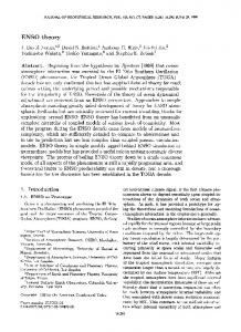
3. Results 3.1. ENSO variability Area-averaged monthly SST anomalies (SSTA) over the Niño3 region (5∘ N–5∘ S, 150∘ –90∘ W) provide an index typically used to represent ENSO variability. Time series of the Niño3 index from HadISST observations and the CESM-GAMIL2 and CESM PI-control runs are compared in Figure 1. The PI-control simulation (years 101–300) from another ‘parent’ model (i.e. FGOALS-g2 from CMIP5) is also included for comparison. Compared with observations, the CESM simulates a much stronger SSTA variation, whereas the CESM-GAMIL2 shows relatively weak variability, and the FGOALS-g2 exhibits a variability most closely matching observations. When quantifying the ENSO amplitude using the Niño3 index standard deviation, the HadISST is approximately 0.81 K, the CESM-GAMIL2 is 0.64 K, the FGOALS-g2 is 0.779 K and the CESM is 1.25 K. Analogous standard deviations based on the Niño3.4 (5∘ N–5∘ S, 160∘ E–150∘ W) index are 0.77, 0.543, 0.778 and 1.22 K, while the Niño4 (5∘ N–5∘ S, 160∘ E–210∘ E) index gives 0.56, 0.40, 0.495 and 0.97 K for HadISST, CESM-GAMIL2, FGOALS-g2 and CESM, respectively. These results show that the ENSO amplitude in CESM is twice as strong as that in CESM-GAMIL2 (the large ENSO amplitudes in CESM were also shown in other studies, e.g. Kang et al., 2014; Bellenger et al., 2014), independent of index selection, and the observation value lies between the two models, while FGOALS-g2 is much closer to observations. Based on this result, ENSO variability is herein represented by the Niño3 index. Previous studies have suggested that ENSO amplitude shows a negative correlation with the strength

© 2015 The Authors. Atmospheric Science Letters published by John Wiley & Sons Ltd on behalf of the Royal Meteorological Society.

Atmos. Sci. Let. 17: 155–161 (2016)

Tracing the source of ENSO simulation differences

157

seasonal cycle in the CESM is more easily disrupted than in CESM-GAMIL2. A dynamical interpretation of the inverse relationship between the annual cycle strength and the ENSO amplitude in the eastern equatorial Pacific, which requires further study using the CESM, is presented by An and Choi (2013) using the Geophysical Fluid Dynamics Laboratory Couple Climate Model (Version 2.0; GFDL-CM2.0).

3.2. Atmospheric feedbacks

Figure 1. Time series of the Niño3 (5∘ N–5∘ S, 150∘ –90∘ W) index for (a) HadISST observations during 1901–2000, (b) CESM-GAMIL2, (c) FGOALS-g2 and (d) CESM during years 101–300 in the PI-control run.

of the annual cycle in the eastern equatorial Pacific because variation in SST for the Niño3 region is generally dominated by both the annual cycle and the ENSO signal (Guilyardi, 2006; An and Choi, 2013). To further understand the ENSO differences, normalized spectra of Niño3 full monthly SST for observation and simulations are calculated, and their corresponding percentages of total spectral energy in annual and semi-annual cycles are presented in Figure 2. Based on observations, the cycle within one year accounts for 35.6% of the total energy. The corresponding values for CESM-GAMIL2 and FGOALS-g2 are 30.7% and 30.1%, respectively; i.e., close to the observed value. In the CESM, however, this value is only 14.4%; i.e. 85.6% of the total energy is available for the interannual signals. These energy distributions indicate that if El Niño is viewed as a disruption of the seasonal cycle (Guilyardi, 2006), then it follows that the weak

On the basis that the only difference between the CESM-GAMIL2 and the CESM is the atmospheric model, atmospheric processes and feedbacks that govern the large difference in ENSO amplitude are explored, with FGOALS-g2 results included for comparison. Atmospheric dynamic and thermal feedbacks in the observation and three simulations are listed in Table 1. Bjerknes feedbacks for the three models compare well in spite of μ being too weak with respect to observations, while heat flux feedbacks, 𝛼, vary significantly. The value for 𝛼 in the CESM is –8.71 W m−2 K−1 , about half of the values of –18.64 and –17.02 W m−2 K−1 simulated in CESM-GAMIL2 and FGOALS-g2, respectively. The latter two are much closer to –16.70 W m−2 K−1 provided by the ERA40 and –15.92 W m−2 K−1 provided by OAFlux. This result may indicate that a weak 𝛼 value means the CESM cannot effectively suppress El Niño warming and thus produces a stronger ENSO. As shown in Table 1, the SW feedback, 𝛼 SW , is the main cause of the 𝛼 difference among the models, although the LH feedback, 𝛼 LH , also plays a role. To further understand the impact of 𝛼 SW on SSTA, a composite analysis of SW flux anomalies and SSTA during El Niño events is performed (Figure 3). Each El Niño event in the models (13 in CESM-GAMIL2, 13 in FGOALS-g2 and 17 in CESM) is defined as an SSTA in Niño3 greater than 1.5 times its standard deviation for at least three consecutive months (Lloyd et al., 2012). Each event in the observation is selected according to the El Niño definition provided by the Climate Prediction Center (Null, 2015), where weak and moderate events are included. In OAFLUX, negative SW anomalies occur at the end of El Niño warming due to the time required to establish a sufficient SST to trigger convection (Guilyardi et al., 2009). In CESM-GAMIL2, negative SW anomalies cover almost the entire warming episode and rapid warming is suppressed, conducive to a weak El Niño. Conversely, for the CESM, large positive SW anomalies occur in the eastern Pacific at the start of an El Niño event, thereby amplifying El Niño development. The evolution of SW anomalies in FGOALS-g2 is closest to that in OAFlux in the eastern Pacific, and correspondingly, the El Niño strength of FGOALS-g2 is much closer to observations. Stronger negative SW anomalies are collocated with weaker positive interannual SSTA in the CESM-GAMIL2 compared with the CESM, consistent with their feedback results obtained by linear regression. In the western and


Atmos. Sci. Let. 17: 155–161 (2016)

158

Y. Tang et al.

Figure 2. Normalized power spectra of full monthly Niño3 SST for (a) HadISST, (b) CESM-GAMIL2, (c) FGOALS-g2 and (d) CESM. The red values indicate the percentage of total spectral energy in the annual and semi-annual cycles, respectively. Table 1. Coefficients of linear regression against SST of the surface net heat flux, shortwave radiation, and latent heat (W m−2 K−1 ); total, convective, and stratiform precipitation (mm day−1 K−1 ); total liquid water path (g m−2 K−1 ); 500 hPa vertical velocity (hPa day−1 K−1 ); and total-, high-, middle-, and low-cloud fraction (% K−1 ) over the Niño-3 region and average annual Bjerknes feedback in the Niño4 region (10−3 N m−2 K−1 ) from observations, CESM-GAMIL2, FGOALS-g2 and CESM, and their Niño3 amplitudes (K). Observation Niño3 𝛼 𝛼 SW 𝛼 LH 𝜇 𝛼 pr 𝛼 prc 𝛼 prl 𝛼 lwp 𝛼 w500 𝛼 cldtot 𝛼 cldhgh 𝛼 cldmid 𝛼 cldlow

0.81 (HadISST)

CESM- FGOALSGAMIL2 g2 CESM 0.64

0.78

1.25

−16.70/−15.92 (ERA40/OAFlux) −18.64 −11.32/−5.63 (ERA40/OAFlux) −11.40 −6.40/−9.50 (ERA40/OAFlux) −9.19 11.06 (ERA40) 8.24 1.11/1.03 (GPCP/CMAP) 1.40 __ 0.90 __ 0.50 19.9/4.42 (SSM/I/ISCCP) 13.47 −9.42 (ERA-40) −11.40 4.52 (ISCCP) 4.78 3.45 (ISCCP) 4.18 2.76 (ISCCP) 3.51 −0.42 (ISCCP) 4.16

−17.02 −9.05 −9.45 8.06 1.14 0.74 0.40 10.55 −9.48 3.67 4.20 2.97 2.41

−8.71 −2.19 −6.20 9.05 1.08 0.95 0.13 10.22 −7.79 3.11 9.00 4.52 −3.34

central Pacific, CESM reproduces the observed evolutions of negative SW anomalies during El Niño development period, while the other two models produce the negative SW anomalies only during mature period. As reported previously, SW flux is associated mainly with the extent of cloud cover, the cloud liquid water path and dynamical circulation. Thus, the SW feedback is decomposed into cloud fraction feedback, LWP feedback and dynamics (vertical velocity at 500 hPa) feedback (Lloyd et al., 2012; Li et al., 2014). The Niño3 averaged feedbacks of the total cloud fraction (𝛼 cldtot ), total LWP (𝛼 lwp ), and dynamics (𝛼 W500 ) in CESM-GAMIL2 are 4.78% K−1 , 13.47 g m−2 K−1 and –11.40 hPa day−1 K−1 , respectively, while in CESM they are 3.11% K−1 , 10.22 g m−2 K−1 and –7.79 hPa day−1 K−1 , respectively. All three component feedbacks contribute to weak SW feedback in the CESM. For FGOALS-g2, both the 𝛼 SW and its three component feedbacks are intermediate between those of the CESM and the CESM-GAMIL2, and are much closer to the latter, suggesting the dominate role of 𝛼 SW in the atmospheric model. Furthermore, the vertical distributions of the cloud fraction and the cloud liquid amount (CLDLIQ) feedbacks (Figure 4) show that in CESM, negative cloud fraction and CLDLIQ feedbacks


Atmos. Sci. Let. 17: 155–161 (2016)


159

Figure 3. Composite El Niño evolution along the equator for the shortwave flux anomaly (shading) and SST anomaly. The contour interval for SST is 0.4 K. (a) OAFLUX (which includes ISCCP radiative fluxes; 1984–2009), (b) CESM-GAMIL2, (c) FGOALS-g2 and (d) CESM.

below 700 hPa are the main causes of weaker 𝛼 cldtot and 𝛼 lwp as well as positive SW anomalies in the eastern Pacific. The too negative cloud fraction feedback and LWP feedback in the lower layers are the common problem in most CMIP5 models, possibly arising from the same root as the ‘too few too bright’ low-cloud problems (Li et al., 2015, pers. comm.). The small stratiform rainfall feedback in models may be one important factor (Li et al., 2014).

4. Discussion and conclusions The ENSO simulations of this study are conducted using two CESM-based GCMs (i.e. CESM and CESM-GAMIL2) that differ only in their atmospheric components. The ENSO amplitudes simulated by the two models are different; e.g. the standard deviation of the Niño3 index in the CESM is up to twice that in CESM-GAMIL2. The strong amplitude in the CESM

is consistent with its weak seasonal cycle strength, which accounts for only 14.4% of the total energy compared with 30.7% in CESM-GAMIL and 35.6% in observations. Less energy within the seasonal cycle indicates that more is available for interannual signals (Guilyardi, 2006). For comparison, another ‘parent’ model (i.e. FGOALS-g2 from CMIP5) is also included, and the differences in the simulations of ENSO amplitude are attributed to differences in two atmospheric feedbacks, i.e., the positive Bjerknes feedback and negative heat flux feedback, with a main contribution from the heat flux feedback. In the CESM, the weak negative heat flux feedback, approximately half the size of the corresponding feedback calculated from observations and the CESM-GAMIL2 simulation, is found to be incapable of effectively dampening El Niño warming, thereby favoring a strong ENSO. Among the four components of heat flux feedback, the SW component is found to be the main cause of weak


Atmos. Sci. Let. 17: 155–161 (2016)

160

Y. Tang et al.

Figure 4. Vertical cross-section of cloud fraction feedback (color shading) and cloud liquid amount (CLDLIQ) feedback (black contours) for (a) CESM-GAMIL2, (b) FGOALS-g2 and (c) CESM averaged over the equatorial Pacific (5∘ N–5∘ S) (units: percent for cloud fraction and 10−6 Kg Kg−1 for CLDLIQ).

heat flux feedback in the CESM, although the LH component also played a role. Further examination indicates that the negative low-cloud fraction feedback and the negative low-cloud liquid amount feedback are the main contributors to weaker 𝛼 SW in the CESM in the Niño3 region; this result may be associated with its small stratiform rainfall feedback (Li et al., 2014). ENSO amplitudes in FGOALS-g2 and CESMGAMIL are moderately different. Therefore, the role of ocean feedbacks in ENSO simulations should be further investigated. In addition, as ENSO simulations are related to their climatological mean state (Guilyardi, 2006), their relationship between the ENSO amplitude and climatological mean state in the CESM and CESM-GAMIL, as well as their uncoupled models, should be explored in future studies. Moreover, the inverse relationship between the mechanism of ENSO amplitude and season cycle merits further investigation. The significance of differences in ENSO amplitude

as well as error bars in longer time scales (such as millennial scale) will also be researched in future.

Acknowledgements We thank Nan Ding and Wei Xue for help in establishing the CESM-GAMIL2. This work was funded by the National Natural Science Foundation of China (No. 41330527) and the Chinese Academy of Sciences Strategic Priority Research Program (Grant No. XDA05110304).

References Adler RF, Huffman GJ, Chang A, Ferraro R, Xie PP, Janowiak J, Rudolf B, Schneider U, Curtis S, Bolvin D, Gruber A, Susskind J, Arkin P, Nelkin E. 2003. The version-2 global precipitation climatology project (GPCP) monthly precipitation analysis (1979–present). Journal of Hydrometeorology 4: 1147–1167. An SI, Choi J. 2013. Inverse relationship between the equatorial eastern Pacific annual-cycle and ENSO amplitudes in a coupled general circulation model. Climate Dynamics 40: 663–675.


Atmos. Sci. Let. 17: 155–161 (2016)


161

Bellenger H, Guilyardi E, Leloup J, Lengaigne M, Vialard J. 2014. ENSO representation in climate models: from CMIP3 to CMIP5. Climate Dynamics 42: 1999–2018. Guilyardi E. 2006. El Niño–mean state–seasonal cycle interactions in a multi-model ensemble. Climate Dynamics 26: 329–348. Guilyardi E, Braconnot P, Jin FF, Kim ST, Kolasinski M, Li T, Musat I. 2009. Atmosphere feedbacks during ENSO in a coupled GCM with a modified atmospheric convection scheme. Journal of Climate 22: 5698–5718. Guilyardi E, Cai W, Collins M, Fedorov A, Jin FF, Kumar A, Sun DZ, Wittenberg A. 2012a. New strategies for evaluating ENSO processes in climate models. Bulletin of the American Meteorological Society 93: 235–238. Guilyardi E, Bellenger H, Collins M, Ferrett S, Cai W, Wittenberg A. 2012b. A first look at ENSO in CMIP5. CLIVAR Exchanges 17: 29–32. Hunke EC Lipscomb WH. 2008. CICE: The Los Alamos sea ice model user’s manual, Version 4, Los Alamos National Laboratory Tech. Rep. LA-CC-06-012, 76 pp. Hurrell JW, Hack JJ, Shea D, Caron JM, Rosinski J. 2008. A new sea surface temperature and sea ice boundary dataset for the community atmosphere model. Journal of Climate 21: 5145–5153. Kang X, Huang R, Wang Z, Zhang RH. 2014. Sensitivity of ENSO variability to Pacific freshwater flux adjustment in the community earth system model. Advances in Atmospheric Sciences 31: 1009–1021. Kim ST, Cai W, Jin FF, Yu JY. 2014. ENSO stability in coupled climate models and its association with mean state. Climate Dynamics 42: 3313–3321. Kim ST, Yu JY. 2012. The two types of ENSO in CMIP5 models. Geophysical Research Letters 39: L11704. Li LJ, Wang B, Zhang GJ. 2014. The role of nonconvective condensation processes in response of surface shortwave cloud radiative forcing to El Niño warming. Journal of Climate 27: 6721–6735. Li LJ, Wang B, Dong L, Liu L, Shen S, Hu N, Sun WQ, Wang Y, Huang WY, Shi XJ, Pu Y, Yang GW. 2013. Evaluation of grid-point atmospheric model of IAP LASG Version 2 (GAMIL2). Advances in Atmospheric Sciences 30: 855–867. Lloyd J, Guilyardi E, Weller H. 2009. The role of atmosphere feedbacks during ENSO in the CMIP3 models. Atmospheric Science Letters 10: 170–176. Lloyd J, Guilyardi E, Weller H. 2012. The role of atmosphere feedbacks during ENSO in the CMIP3 models. Part III: the shortwave flux feedback. Journal of Climate 25: 4275–4293. McPhaden MJ, Zebiak SE, Glantz MH. 2006. ENSO as an integrating concept in earth science. Science 314: 1740–1745. Neale RB, Richter JH, Jochum M. 2008. The impact of convection on ENSO: From a delayed oscillator to a series of events. Journal of Climate 21: 5904–5924. Neale RB, Richter J, Park S, Lauritzen PH, Vavrus SJ, Rasch PJ, Zhang M. 2013. The mean climate of the community atmosphere model (CAM4) in forced SST and fully coupled experiments. Journal of Climate 26: 5150–5168. Null J. 20157-11-04. El Niño and La Niña Years and Intensities. http://ggweather.com/enso/oni.htm (accessed 10 March 2015).

Oleson KW, Lawrence DM, Bonan GB, Flanner MG, Kluzek E, Lawrence PJ, Levis S, Swenson SC, Thornton PE, Dai A, Decker M, Dickinson R, Feddema J, Heald CL, Hoffman F, Lamarque JF, Mahowald N, Niu GY, Qian T, Randerson J, Running S, Sakaguchi K, Slater A, Stöckli R, Wang A, Yang ZL, Zeng X, Zeng X. 2010. Technical description of version 4.0 of the Community Land Model (CLM), NCAR Tech. Note NCAR/TN-478+STR, 257 pp. Rossow WB, Schiffer RA. 1999. Advances in understanding clouds from ISCCP. Bulletin of the American Meteorological Society 80: 2261–2288. Smith RD, Jones P, Briegleb B, Bryan F, Danabasoglu G, Dennis J, Dukowicz J, Eden C, Fox-Kemper B, Gent P, Hecht M, Jayne S, Jochum M, Large W, Lindsay K, Maltrud M, Norton N, Peacock S, Vertenstein M, Yeager S. 2010. The Parallel Ocean Program (POP) reference manual, Los Alamos National Laboratory Tech. Rep. LAUR-10-01853, 140 pp. Sun DZ, Yu Y, Zhang T. 2009. Tropical water vapor and cloud feedbacks in climate models: a further assessment using coupled simulations. Journal of Climate 22: 1287–1304. Uppala SM, Kållberg PW, Simmons AJ, Andrae U, Bechtold VDC, Fiorino M, Gibson JK, Haseler J, Hernandez A, Kelly GA, Li X, Onogi K, Saarinen S, Sokka N, Allan RP, Andersson E, Arpe K, Balmaseda MA, Beljaars ACM, Van De Berg L, Bidlot J, Bormann N, Caires S, Chevallier F, Dethof A, Dragosavac M, Fisher M, Fuentes M, Hagemann S, Hólm E, Hoskins BJ, Isaksen L, Janssen PAEM, Jenne R, Mcnally AP, Mahfouf JF, Morcrette JJ, Rayner NA, Saunders RW, Simon P, Sterl A, Trenberth KE, Untch A, Vasiljevic D, Viterbo P, Woollen J. 2005. The ERA-40 Re-Analysis. Quarterly Journal of the Royal Meteorological Society 131: 2961–3012. Wang B, Wang H, Ji ZZ, Zhang X, Yu RC, Yu YQ, Liu HT. 2004. Design of a new dynamical core for global atmospheric models based on some efficient numerical methods. Science China. Mathematics 47: 4–21. Wang C, Deser C, Yu JY, DiNezio P, Clement A. 2012. El Nino and Southern Oscillation (ENSO): A Review, A Chapter for Springer Book: Coral Reefs of the Eastern Pacific. Springer-Verlag. Watanabe M, Chikira M, Imada Y, Kimoto M. 2011. Convective control of ENSO simulated in MIROC. Journal of Climate 24: 543–562. Weng F, Grody N, Ferraro R, Zhao Q, Chen C. 1997. Global cloud water distribution derived from special sensor microwave imager/sounder and its comparison with GCM simulation. Advances in Space Research 19: 407–411. Xie P, Arkin PA. 1997. Global precipitation: a 17-year monthly analysis based on gauge observations, satellite estimates, and numerical model outputs. Bulletin of the American Meteorological Society 78: 2539–2558. Yu L, Weller RA. 2007. Objectively analyzed air–sea heat fluxes for the global ice-free oceans (1981–2005). Bulletin of the American Meteorological Society 88: 527–539. Yu JY, Kim ST. 2010. Identification of Central-Pacific and Eastern-Pacific types of ENSO in CMIP3 models. Geophysical Research Letters 37: L15705.


Atmos. Sci. Let. 17: 155–161 (2016)