Track Before Detect Algorithm for Tracking Extended Targets applied ...

Track Before Detect Algorithm for Tracking Extended Targets applied to Real-World Data of X-band Marine Radar B. Errasti-Alcala and P. Braca NATO STO CMRE La Spezia, Italy {errasti, braca}@cmre.nato.int Abstract—This communication presents the application of a Track before Detect technique for tracking extended targets in cluttered environment using a high resolution marine radar. The algorithm makes use of a particle filtering approach and assumes that the target shape is an ellipse. We compute numerically the posterior probability of the target presence jointly with the estimation of the target state, augmented with its geometrical parameters (length and width), that could be used for target classification. The results of tests with real-world data are reported, and a comparison, when possible, with the ground truth is also provided.

number of sensors, as a mixture of as many Gaussian components as the true number of targets. These Gaussian functions become progressively narrower and peakier around the true target states in a way that is ruled by the Fisher information [9]. In other words, the PHD is asymptotically optimal increasing the number of sensors. The PHD is suitable to deal with a cluttered environment and with appearing/disappearing moving targets without using track-management logics. The PHD filter can be enhanced in order to deal with the case of extended targets, e.g. see [11]–[14].

Keywords—Multiple target tracking, track before detect, extended targets, real-world experimental results, sequential Monte Carlo methods, Linear Frequency Modulated Continuous Wave

Most of these methods are based on the availability of contacts or thresholded data, which results in a possible loss of information. Track before detect (TbD) techniques are designed to process unthresholded measurements. These techniques make use of the whole available information and the detection stage is incorporated in the tracker [15], [16]. As a consequence, no information is lost due to the thresholding stage, however, on the other hand a more demanding computational effort is required.

I.

I NTRODUCTION

Traditional target tracking bases its principle on the processing of point detections. The low resolution of former sensors made the target appear in one single resolution cell, but high resolution sensors allow the target to be found in several cells, providing what is called an “extended target” or “extended object”. The most primitive techniques to deal with an extended target consisted on computing its centroid and considering a punctual detection, but several methods have been proposed for extended target tracking, or for the tracking of a group of targets [1]. Most of the approaches for extended target tracking are based on sequential Monte Carlo methods. In [2], the extended object is considered as a set of fixed points in a target reference frame. The probabilistic detection of this points lead to a data association problem which is solved by means of augmenting the target’s state vector with the association hypothesis. In [3], the authors propose two different methods: An interacting multiple model data augmentation and a modified version of the mixture Kalman filter. In both cases, the kinematic state of the target and the modal state are estimated separately, providing a reasonable tradeoff between computational effort and performance. In [4], a Bayesian filter for joint detection and estimation of an extended object is proposed. A thorough review of Monte Carlo methods for extended target tracking may be found in [5]. Among the several emerging target tracking methodologies one of the most popular is the probability hypothesis density (PHD) filter [6], [7]. Indeed, in [8]–[10] authors have proven that the multi-sensor PHD function behaves, by increasing the

This communication presents the use of a TbD algorithm based on a particle filter (PF) that estimates the geometric shape of targets, considered elliptical, as well as their kinematic properties. The method is applied on real-world data and its validity is assessed by comparing its outcome with ground truth information derived by the automatic identification system (AIS) [17]. In [18] there are further details about the use of the AIS as ground truth. The radar has a narrow beam rotating antenna and uses Linear Frequency Modulated Continuous Wave (LFMCW) [19]. The radar mixes the received echo with the transmitted waveform and low-pass filters the result before the baseband ADC sampling. The High Resolution Range Profiles (HRRP) are the obtained as the FFT of the raw data. The radar system used to validate the featured algorithm is one node of the Radar Sensor Network (RSN), a coherent bistatic X-band radar system installed at the Gulf of La Spezia, Italy. The RSN consists of two fully configurable synchronized radar nodes, the aforementioned Marine node and an ISAR imaging node. The low transmitted power (up to 5 watts, CW) simplifies the electronics and reduces the probability of intercept, while maintaining a high performance due to pulse compression techniques. The network is a compact, fast deployable and scalable system used for research, surveillance of small crafts in short and medium ranges, and offshore and port protection.

The Marine node is configurable in terms of central frequency, bandwidth, Pulse Repetition Frequency, transmitted power, speed of rotation and receive attenuation. The remainder of this communication is organized as follows: Section II formulates the problem and the presents the tracking method. Section III shows the experiment configuration and the results and section IV presents the conclusion.

of raw radar frames. Each frame is a grid of range-bearing cells containing the value of the reflected signal. The method is based on particle filtering [20]. In this section the target’s motion, the measurement model and the estimation procedure used by the particle filter are presented. A. Target Model As in [21], [22], where random matrices are used to model the shape of the target, an elliptic geometry is assumed here. A constraint has been added, making the target’s long axis parallel to its speed vector. As a consequence, the target’s state x = [x, y, x, ˙ y, ˙ l1 , l2 ]T is a 6 element vector, where (x, y) represents the position of the target, (x, ˙ y) ˙ represents the speed and l1 and l2 are the length and width of the target i.e. long and short axes of the ellipse, respectively. The motion of the target is modeled as a Markovian process, in particular the Nearly Constant Velocity model [1]. The target dynamics are given by

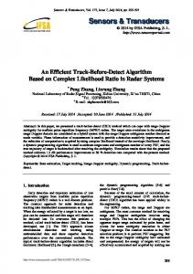
(a) Map of the area acquired by the radar

xn+1 = f (xn ) + g(xn , wn ),   1 0 T 0 0 0 0 1 0 T 0 0   0 0 1 0 0 0 f (xn ) =  x , 0 0 0 1 0 0 n 0 0 0 0 1 0 0 0 0 0 0 1  2  T 0 0 0  2 2   0  0 T2 0 0  σax   0 σay T 0 0 0   g(xn , wn ) =  · 0 T 0 0 0  0 0  0 0 0 σl1 0 0 0 0 σl2

(1)

(2)

 0 0 0 0 w , 1 0 n 0 1

(3) where T is the sampling period, σl1 and σl2 are the typical deviations of the length and width of the target respectively, σax,y is the acceleration standard deviation along x and y, respectively. The term wn indicate a four element random vector, whose elements are Gaussian distributed with zero mean and identity covariance matrix. Although the real length and width of a target are fixed, in this Bayesian framework it is necessary to assume that they can randomly oscillate. The presence or absence of the target is modeled following a binary Markovian process Pr (mn+1 Pr (mn+1 Pr (mn+1 Pr (mn+1

= 0 | mn = 0 | mn = 1 | mn = 1 | mn

= 0) = 1 − qb = 1) = qd = 0) = qb = 1) = 1 − qd ,

(4) (5) (6) (7)

(b) One frame of the radar acquisition Fig. 1. Maps of the area illuminated by the radar and its corresponding acquisition. The dyke, the land and other structures can be seen in both maps.

II.

P ROBLEM F ORMULATION

The objective is to sequentially estimate the probability of having a target and its kinematic properties along with its length and width. The available information is a sequence

where mn is the modal state and takes the value 0 when the target is not present and the value 1 when the target is present, qb is the probability of the target appearing and qd is the probability of the target disappearing. At instant n, the state of the system, and thus the state kept by the particles, is the union of both, the vector xn and the modal state mn . A system that evolves following this model is said to follow a Markovian jump model [23], [24].

Parameter Central Frequency Bandwidth Pulse Repetition Frequency Baseband Sampling Frequency Antenna Rotation Speed Transmitted Power Attenuation at receive Range Resolution Angular Precision Antenna Azimuth Aperture Polarization

B. Measurement Model The measurement model assumes that the received power is exponentially distributed in each range-bearing cell (i, j) The value of the distribution parameter λ is selected according to the expected value of the clutter in the cells where the target is not present, and according to the expected value of the target’s radar return if the target is present. In each cell, the parameter λ of the exponential distribution is the inverse of the expected power. Measured power in each cell is considered conditionally independent from measures in other cells. n o zn = zn(i,j)

i,j

( zn(i,j) ∼

= h(xn , m),

(8)

(i,j)

Exp(λ1 ) if m = 1, I(i, j) = 1, (i,j) Exp(λ0 ) otherwise,

(9)

(10) (11) (12) (13)

C. Likelihood Function and Estimation Procedure The likelihood function p (z | x, m) is based on the measurement model and under the assumption of conditionally independent cell measurements,
p z(i,j) | x, m

(14)

(i,j)

it is computed as the product of the individual likelihoods for each cell Y (i,j) (i,j) (i,j) p (z | m = 0) = λ0 e−λ0 z (15) (i,j)

Y

p (z | x, m = 1) =

(i,j) −λ(i,j) z (i,j) 1

λ1

e

(16)

(i,j):I(i,j)=1

×

Y (i,j):I(i,j)=0

(i,j) −λ(i,j) z (i,j) 0

λ0

e

The posterior distribution of the target state xn , mn can be numerically reconstructed by a particle filtering strategy [15], [16], [20] which use the statistical model defined by the likelihoods (15)-(16), then we have Np X

wn(p) δ(x(p) ,m(p) ) (xn , mn ) , n

n

p=1

where I(·) is the indicator function. If the target is present in the surveillance region (m = 1) and occupies the cell (i,j) (i, j) then zn is distributed as an exponential with parameter (i,j) (i,j) is distributed as an exponential with λ1 . Otherwise, zn (i,j) parameter λ0 . We formally say that the target occupies the cell (i, j) if the vector of the difference between the target’s centroid (x, y) and the cell location (x(i, j), y(i, j)), rotated by the target’s course φ and normalized with N , is lower than unity. One full measurement zn of the whole scanned area is available every T seconds.

Y

PARAMETERS OF THE RADAR ACQUISITION

p (xn , mn | z1 , . . . , zn ) ≈

where we have defined    

x(i, j) − x