Jan 5, 2016 - c 2016 Norwegian Society of Automatic Control ... invariant representation is not as great as in the gen- eral case. However, the kinematic ...
Modeling, Identification and Control, Vol. 37, No. 1, 2016, pp. 53–62, ISSN 1890–1328
Tracking a Swinging Target with a Robot Manipulator using Visual Sensing Torstein A. Myhre 1 Olav Egeland 1 1
Department of Production and Quality Engineering, NTNU. NO-7491 Trondheim, Norway. {torstein.a.myhre,olav.egeland}@ntnu.no
E-mail:
Abstract In this paper we develop a method for loading parts onto a swinging target using an industrial robot. The orientation of the target is estimated by a particle filter using camera images as measurements. Robust and accurate tracking is achieved by using an accurate dynamic model of the target. The dynamical model is also used to compensate for the time delay between the acquisition of images and the motion response of the robot. The target dynamics is modeled as a spherical pendulum. To ensure robust visual tracking the position of the target mass center is estimated. The method is experimentally validated in a laboratory loading station with a swinging conveyor trolley as target, which is commonly used in industry. Keywords: Industrial Robots, Particle Filter, Computer Vision for Manufacturing
1 Introduction Robot vision in industrial applications is typically used where work objects are static or moving at constant velocity, such as when picking from a conveyor belt. A more demanding task is the loading of objects on a swinging conveyor trolley, which is illustrated in Figure 1. In the usual industrial solution objects are loaded on the trolleys manually because they are swinging freely. They are swinging freely to avoid excessive forces and accelerations. This paper presents a method to perform this task automatically, by real-time control of an industrial robot manipulator using an estimate of the trolley orientation computed from camera images with a particle filter. The controller interfaces of industrial robots are designed to operate at fixed update rates, which can range from 125 Hz (Universal Robots), 250 Hz (KUKA) and up to the kHz level. However, cameras that are used in computer vision applications typically have lower update rates. They are limited by the camera hardware itself and the bandwidth available for image transfer. The images are often transferred using Eth-
doi:10.4173/mic.2016.1.5
ernet or USB, which provides no guarantees of realtime performance by default. These limitations are described in Corke and others (1996) as the “dynamics of visual sensing”. Clearly, for a fixed-rate robot controller to work with the varying frame rates provided by cameras, some method must be employed to compensate for delays and interpolate between images. An approach to compensate for these effects was proposed in Wang et al. (2013), using a dual-rate Kalman filter. A dynamic model was used to predict the target motion at the time instants required for robot control. In Wang et al. (2015) and Lin et al. (2013) it was proposed to identify the parameters of the dynamical model using Expectation-Maximization. Since the work Isard and Blake (1998) many authors have explored the use of particle filters for visual object tracking. For robotic visual servoing it is specially interesting to look at the work on tracking of rigid bodies in Cartesian space. Particle filter based tracking on the SE(3) group has been investigated using different assumptions on the underlying dynamical model in Kwon et al. (2007), Choi et al. (2011) and Choi and Christensen (2012). In particular, the particle filters were
c 2016 Norwegian Society of Automatic Control
Modeling, Identification and Control
Figure 1: Manual loading of objects onto a swinging conveyor trolley is a common task in industry. The proposed automatic solution is to control the trajectory of the robot manipulator in real-time using an estimate of the trolley motion. An estimate of the trolley motion is found using particle filter based visual tracking.
designed to account for the properties of SE(3). The kinetics were modeled as random walk or with an autoregressive dynamic model. To develop this further, we belive that it may be an advantage to use a kinetic model based on the physical equations of motion. This was done in our previous work Myhre and Egeland (2015) where the dynamics of a spherical pendulum was used. A potential benefit of a physical model is that the assumed noise level in the particle filter can be significantly reduced. One of the challenges in visual tracking is to achieve accuracy despite occlusions and cluttered scenes. A possible solution is to use multiple cameras as in Lippiello et al. (2007) and Kermorgant and Chaumette (2011). In recent years researchers have demonstrated that particle filter based visual tracking can be used in the robot feedback loop Ibarguren et al. (2014), Chitchian et al. (2013), even though it is considered as a computationally heavy method. The parallel nature of the filter makes it possible to run them on commodity Graphical Processing Units (GPUs) to achieve good performance Choi and Christensen (2013), Concha et al. (2014) and Pauwels et al. (2013). A dynamical model based on physical principles needs to have accurate parameters in order to be useful. This can be done with parameter estimation. An overview of methods for parameter estimation based on particle filtering can be found in Kantas et al. (2009). The two main on-line approaches are Expectation-
54
Maximization Sch¨on et al. (2011) and gradient ascent Poyiadjis et al. (2011). We used the approach Poyiadjis et al. (2011) in our previous work Myhre and Egeland (2015) to find accurate parameters of a spherical pendulum during visual tracking. This is further developed in the following. In this paper we propose a method to perform the task illustrated in Figure 1, namely to control a robot manipulator tracking a swinging target using computer vision. The proposed method uses a model based on physical principles with estimated parameters, namely the center of mass position, which enables the robot to accurately track the target even as it accelerates. This is experimentally demonstrated in Section 5. The method proposed in this paper has the same goal as in Lin et al. (2013), which is to compensate for visual sensing dynamics using a model of the motion of the target object. The method presented in Lin et al. (2013) uses a general dynamic model, while we propose to use a physically based dynamical model of a spherical pendulum in order to achieve high performance for the specific application. In this paper XYZ Euler angles was chosen for the kinematic representation of rotation. The main motivation for this is to simplify and improve the parameter estimation algorithm. The benefits of a coordinate invariant representation with the particle filter was thoroughly discussed in Kwon et al. (2007). In the use case that is presented in this paper, it is unrealistic to consider swinging motions with amplitudes larger than 10◦ , so the benefits of using a coordinate invariant representation is not as great as in the general case. However, the kinematic convention chosen in this paper has the benefit that the center of mass position naturally can be described using two angular offsets and one linear offset. This enables the parameter estimator to identify the accurate value of the two angular offsets, even when the target is hanging with no velocity (stationary), in which case it is impossible to identify the correct value of the linear offset. In the case of a stationary target, only the two angular offsets are required for visual servoing. A coordinate-free version may be the topic of future research. This paper presents a novel method for accurate tracking of a swinging target with an industrial robot. 1. The proposed method can handle both stationary and moving targets. 2. A two stage control system is proposed, where one part is running at the rate at which the cameras can deliver images, while the other part is running at the rate required by the robot motion controller. The two stages are connected using a prediction module based on an accurate dynamical model of the swinging target.
Myhre and Egeland, “Tracking a Swinging Target with a Robot Manipulator using Visual Sensing” 3. Experiments are performed to demonstrate that where δ(·) is the Dirac delta function, wk(i) are scalar the method can be used for automatic loading of weights and x(i) ∈ Rn . k parts onto the swinging target, using a laboratory The specific particle filter used in this paper is known version of a loading station found in industry. as Sequential Importance Sampling with Resampling 4. The experiments are performed using standard which is described in detail in e.g. Capp´e et al. (2007) and Doucet and Johansen (2011). commercial equipment. A numerical approximation to the expected value of The structure of the paper is as follows: In Section 2 p(xk |I1:k ) can be found as we discuss the preliminaries of particle filtering and paZ N rameter estimation, in Section 3 we present a dynamic X (i) (i) xk p(xk |I1:k )dxk ≈ wk xk . (6) model and observation model used for tracking, in Seci=1 tion 4 we propose a method for using the state estimate to control an industrial robot manipulator in real-time. Experiments that validate the proposed method are 2.2 Estimation of Static Parameters presented in Section 5. Methods for sequential estimation of static parameters using particle filters have recently been developed Kantas et al. (2014). An online gradient ascent method is 2 Preliminaries used here, In this paper we consider a non-linear system with adθk+1 = θk + Γ∇θ log p(Ik |I1:k−1 ), (7) ditive Gaussian noise xk = Fd (xk−1 , θ) + vk
(1)
where
Γ ∈ R3×3 . (8) where xk ∈ R is the state vector at time step k, θ is a vector of static parameters and vk ∼ N (0, Σ) is a Using the approach presented in Poyiadjis et al. noise vector. The probability density of (1) is known (2011) a set of vectors α(i) is found such that k as the transition density and can in the case of additive N N Gaussian noise be written as X X (i) (i) (i) (i) ∇θ log p(Ik |I1:k−1 ) ≈ wk αk − wk−1 αk−1 . f (xk |xk−1 ) = N (xk − Fd (xk−1 , θ), Σ). (2) i=1 i=1 (9) An observation is made at each time step k by a camera (i) The vectors α are given by the recursive expression k taking an image, denoted by Ik . The relation between n
Ik and xk is given by the observation density g(Ik |xk ), which is given in Section 3.2. In this section we first present a particle filter for estimation of the state xk , then a method for estimating the vector of static parameters θ, based on the sequence of camera images.
N P (i)
αk =
j=1 N P k=1
(j)
(i)
(j)
wk−1 f (xk |xk−1 ) (j)
(i)
(j)
wk−1 f (xk |xk−1 )
� (j) × αk−1 +
(10)
� (i) (j) (i) ∇θ log f (xk |xk−1 ) + ∇θ log g(Ik |xk )
2.1 Particle Filter
Inferences about the state vector at timestep k can be where ∇θ log f (xk |xk−1 ) and ∇θ log g(Ik |xk ) are gramade using the prediction equation dients of the transition (2) and observation (29) densiZ ties respectively, as developed in the next section. p(xk |I1:k−1 ) = f (xk |xk−1 )p(xk−1 |I1:k−1 )dxk−1 (3) and the update equation p(xk |I1:k ) = R
g(Ik |xk )p(xk |I1:k−1 ) . g(Ik |xk )p(xk |I1:k−1 )dxk
(4)
3 Modeling 3.1 Kinematic and Dynamic Modeling
The dynamics of the system is modeled as a spherical These equations are intractable in general, but parti- pendulum with one additional degree of freedom decle filters are efficient methods for computing numerical scribing the rotation about the pendulum axis. The configuration can then be described by the XYZ Euapproximations ler angles φx , φy and φz . When a workpiece is atN X (i) (i) p(xk |I1:k ) ≈ wk δ(xk − xk ), (5) tached to the hanger, the center of mass will be shifted, and the equilibrium position of the hanger will have i=1
55
Modeling, Identification and Control while the vector of unknown parameters is
zW
zB
Camera reference frame C
x
B
θ2
θ3
�T
.
(15)
The velocity components in (14) are affected by additive noise, modeled by
u
xW
zC
� vk = 0
0
0
vk1
vk2
vk3
�T
,
where the components
xC v
vk1 ∼ N (0, σ12 ), vk2 ∼ N (0, σ22 ), vk3 ∼ N (0, σ32 ) (16)
Image plane
yC
� θ = θ1
Figure 2: The body reference frame B is rotating relative to the inertial reference frame W. The geometric trolley model is described by a list of line segments in R3 .
are samples from Gaussian distributions. A continuous state space model is found from equations (13), (14) and (15) as x˙ = F (x, θ).
(17)
The model is discretized in time using the first order Euler method giving Fd (xk−1 , θ) in the system (1). an unknown offset. To account for this uncertainty, The gradient ∇θ log f (xk |xk−1 ) is required for pawe include offset angles θ1 and θ2 about the x and y rameter estimation in Section 2.2. Let axes, so that the Euler angles become Φx = φx + θ1 , Φy = φy + θ2 and φz . Here θ1 and θ2 are constant Ξ = diag(0, 0, 0, 1/σ12 , 1/σ22 , 0), (18) unknown parameters to be identified. As shown in Figure 2 the world frame is denoted W, then since the transition density is Gaussian, and the body-fixed frame is denoted B. The rotation ∇θ log f (xk |xk−1 ) = matrix from W to B is then given by (19) (xk − Fd (xk−1 , θ))T Ξ∇θ Fd (xk−1 , θ), W RB = Rx (φx + θ1 )Ry (φy + θ2 )Rz (φz ). (11) In the stationary position of the pendulum we have that φx + θ1 = 0 and φy + θ2 = 0. The equations of motion are derived using the EulerLagrange equations applied to the Lagrangian L=
� 1 2 T mθ3 r˙ 3 r˙ 3 − mgθ3 0 2
0
� 1 r3
(12)
where θ3 is the unknown constant distance from the pendulum attachment point to �the center of�mass, and W r3 is the last column in RB = r1 r2 r3 . The distance θ3 is the third unknown parameter to be identified. The resulting equations of motion are φ¨x φ¨y φ¨z
2φ˙ x φ˙ y θ3 sin 2Φy + 2g sin Φx cos Φy = θ3 cos 2Φy + θ3 g 1 = sin Φy cos Φx − φ˙ 2x sin 2Φy θ3 2 =0
56
φy
φz
φ˙ x
φ˙ y
φ˙ z
�T
∇θ Fd (xk−1 , θ) =
Z
tk
tk−1
∂F (x, θ) ∂x ∂F (x, θ) + dt. ∂x ∂θ ∂θ (20)
3.2 Image Model
It is assumed that the object is a rigid body with orienW tation given by the rotation matrix RB , as illustrated W 3 in Fig. 2. A point p ∈ R in frame W is given in frame B using (13) W B pW = RB p . (21) The transformation from the frame W to C is given by
where g = 9.81 m s−2 is the acceleration of gravity. The state vector of the system (1) is � x = φx
where ∇θ Fd (xk−1 , θ) is the sensitivity with respect to the parameters θ. The sensitivity is an estimate of the effect variations in the parameter θ has on Fd (xk−1 , θ). From Khalil (2002) the sensitivity is computed by taking derivatives of (17) with respect to the parameters θ and solving this ode
C pC = RW pW + tCW .
(22)
The image is a two dimensional array of pixel inten� �T (14) sities I(p) where p = u v and u and v are pixel
Myhre and Egeland, “Tracking a Swinging Target with a Robot Manipulator using Visual Sensing” coordinates in the image plane. The camera calibration matrix is kx 0 ku (23) K = 0 ky kv 0 0 1 where kx , ky , ku and kv are intrinsic camera calibration � �T parameters. Given a point pC = px py pz , the coordinates of the point in the image plane is given by u kx 0 ku px pz v = 0 ky kv py (24) 1 0 0 1 pz or
Ik State and parameter estimator
θ ˆk x
Predictor
ˆ x(t)
qd
Robot Program Reflexxes Motion and Inverse W and Kinematics Ed Compensation
Figure 3: The modules comprising the control system. The modules in the blue box are running at the frame rate determined by the cameras. in vector form. The modules in the red box are running at The methods used to find the intrinsic camera pathe fixed rate required by the robot manipurameters kx , ky , ku and kv and the extrinsic camera lator (125 Hz for UR5). C C parameters RW and tW are described in Section 5. pz p˜ = KpC
(25)
3.2.1 Trolley Frame Visual Model
gives a distance between the points of approximately 5 The visual model of the trolley is given by Ng line pixels. The parameter vector θ does not enter into the obsegments. Each line segment j is specified by its endB B servation density, which means that points pj and qj . For each particle i the rotation (i)
W is computed using the state vector xk . matrix RB The two points in the image plane corresponding to pB j and qjB are found in homogeneous pixel coordinates as C W B p˜j = K(RW RB pj + tW C )
∇θ log gθ (Ik |xk ) = 0.
(30)
4 Control System
(26)
In this section we describe a control system used for automatic loading of parts on the swinging trolley. The B B The line segment defined by pj and qj is found control system structure is visualized in Figure 3. The in pixel coordinates as the line segment from p˜j to content of the block containing “State and parameter q˜j , and can be described as the homogeneous vector estimator” was described in Section 2.1 and 2.2. The � �T mean of the state estimate is computed at each time `˜j = a b c , which is found from the cross prodstep k Z uct Hartley and Zisserman (2003) ˆ k = xk p(xk |I1:k )dxk x (31) `˜j = γS(q˜j )p˜j (28) using (6). The contents of the remaining blocks are where S(q˜j ) is the skew symmetric form of q˜j . A scal- described in the following. ing factor γ is used to ensure that the two dimensional � �T vector nj = a b is a unit vector. It is noted that 4.1 Visual Sensing Dynamics in this description the vector nj is the normal vector Compensation to the line segment in image coordinates. The following observation density is proposed for the The control system illustrated in Figure 3 is logically particle filter: divided into two parts running at different rates. The modules inside the red dotted polygon are running at Ng X the fixed rate required by the robot controller, while g(Ik |xk ) = (I(pj ) − I(pj + λnj ))2 (29) the modules inside the blue dotted rectangle are runi=0 ning at the camera rate. As cameras typically come where pj is the two-dimensional version of the homoge- without real-time guarantees, and the frame rate is neous vector p˜j , nj is the normal vector to line segment typically lower than of the robot motion control sysj, and λ is a parameter which was set to λ = 5, which tem, there is a mismatch between the robot controller C W B q˜j = K(RW RB qj + tW C ).
(27)
57
Modeling, Identification and Control rate and the camera rate. In order to bridge the gap between the modules running at different rates, the “Preˆk dictor” module uses the most recent state-estimate x and parameter estimate θ, to predict the trolley state ˆ at the time instants required to compute set-points x(t) for the robot motion controller. The predictor module predicts the trolley state by integrating the system in (17) Z t ˆ = F (x, θ)dt. (32) x(t) tk
The result is the predicted transform ˆ predicted state x(t).
TBW
qj
qj+1
qj+2
qj+3
qj+4
qj+5
...
ˆ x(t)
...
ˆk x
ˆ k+1 x
ˆ k+2 x
Ik
Ik+1
Ik+2
...
based on the Figure 4: Timing of state estimates xk in the camera rate (blue box) and the desired joint variables qj in the robot controller rate (red box).
4.2 Robot Program and Motion Compensation In order to move the end-effector smoothly between two B B B reference frames T1B = (R1B , tB 1 ) and T2 = (R2 , t2 ) we define the end-effector reference trajectory � � 1 R2B β(s) , R1B exp log RB � EdB (T1B , T2B , s) = B B (tB 2 − t1 )β(s) + t1 (33) where exp(·) is the exponential map so(3) → SO(3) and log(·) is the inverse as defined in Murray et al. (1994). A monotonic function β(s) ∈ [0, 1] is used for interpolation of frames such that excessive acceleration is avoided. We use a linear function of the Logistic function 1 − b. (34) β(s) = a 1 + exp (−ks) where a and b are choosen so that β(0) = 0 and β(1) = 1. The motion of the end-effector is computed using the predicted transform TBW EdW = TBW EdB .
(35)
4.3 Reflexxes and Inverse Kinematics The Reflexxes motion libraries Kr¨ oger (2011) was used in Cartesian space to filter low amplitude high frequency noise that is part of the particle filter estimate. Set-points for the robot joint controller was thereafter computed using an inverse kinematics procedure.
5 Experiments 5.1 Laboratory set-up As shown in Figure 1 a laboratory set-up was built to perform the experiments described in this section. The set-up consisted of two Prosilica GC 1020 Ethernet cameras streaming images to a computer at approximately 35 Hz, which is the fastest they can deliver images at full resolution (1024 × 768 pixels). 58
...
The computer had a Intel i7-3820 CPU, 16 Gb RAM and a Nvidia Titan graphics card, running Ubuntu Linux 14.10. The Precision Time Protocol was used to achieve synchronization between the clock on the two cameras and the clock on the computer controlling the robot. A chessboard was mounted on the robot end-effector in order to find the camera calibration parameters required in Section 3.2. For each camera 26 pictures were taken of the chessboard with the robot end-effector in different poses. The intrinsic camera parameters kx , ky , ku and kv were found using standard camera calibration methods provided by the OpenCV library described in Bradski and Kaehler (2008). The extrinsic C and tCW were found using the camera parameters RW method described in Park and Martin (1994). The distance from each of the cameras to the trolley frame was approximately 2.2 m. The differential equations (13) and (20) were discretized using the Euler method. To achieve an accurate estimate of the parameter vector θ it is important that the sensitivity estimate in (20) is accurate. Therefore the step-size for integration was set to 0.0002 s. The two most computationally intensive parts of the particle filter are the observation model and the dynamical model, which therefore were implemented in CUDA in order to run them on the GPU of the Nvidia Titan graphics card.
5.2 Visual Sensing Dynamics Compensation The experiment in this section was performed to validate the performance of the visual dynamics sensing compensation described in Section 4.1. A 5 s sequence of the state estimate was recorded while the target was swinging, and the resulting φx component is shown in Figure 5. The graphs show that the output from the
Myhre and Egeland, “Tracking a Swinging Target with a Robot Manipulator using Visual Sensing” 3.0
φx [Deg]
2.5 2.0 1.5 1.0 0.5 0.0 15
16
17
18
19
20
Time [s] 1.0
φx [Deg]
φx [Deg]
2.9
2.5
2.1
The motions that were performed in the experiments are shown in Figure 7. The cylindrical object carried by the robot had inner diameter 22 mm. The trolley frame was welded from steel bars with a square cross section (8 mm×8 mm). The robot program is described in Figure 6. Step 1) Estimate the parameter vector θ.
0.5
Step 2) Set the time variable t = 0 and start tracking using the found parameter vector θ.
0.0 15.5
15.7 Time [s]
15.9
16.1
16.4
16.6 Time [s]
16.8
17.0
Figure 5: The figure shows the discrete-time state estimate of φx (in blue), which is updated at the camera rate, and the predicted state (in red), which is in the faster robot rate of 125 Hz. predictor module provide a smoother and more accurate estimate of the target state, than the estimate coming directly from the state estimator.
Step 3) Move the end-effector from the initial position to the pose T1B when t ∈ [0, 15). Step 4) Move the end-effector according to EdB (T1B , T2B , s(t)), where (t − 15)/5 if 15 ≤ t < 20 s(t) = 1 if 20 ≤ t < 25 (36) (25−t) if 25 ≤ t < 30 5 Figure 6: Robot program.
5.3 Case Study: Part Loading In this section we present the experimental validation of the proposed method. We decided to do this by synchronizing the motion of the robot and the trolley, and then using the robot to place a hollow cylinder in loading position. Instead of releasing the grip on the cylinder, the robot then removed the cylinder from the loading position. The idea was then that if the robot could do this without the cylinder coming into contact with the trolley, the synchronization would be accurate within the difference in dimension of the hole in the cylinder and the size of the attachment hook on the trolley. In this case the documented accuracy would be 6 mm. The target was a trolley hanging from an overhead conveyor, which is used in industrial loading stations commonly operated with manual labour. The experiment was designed to demonstrate that the proposed method also can handle the situations where the position of the mass center changes as objects are attached to the trolley, and that this can be achieved both with moving and stationary targets. To this end, an object was loaded on the trolley so that the center of mass changed to an unknown position, which was estimated by the parameter estimation algorithm. Then the synchronization of robot and trolley motion was demonstrated by letting the robot move the hollow cylinder into loading position and back again without touching the trolley. In this motion the cylinder is very close to the trolley, and a synchronization of 6 mm is validated if the cylinder does not touch the trolley.
The program was first executed with a stationary target. The results are shown in Figure 8a. In Step 1 the values of the parameters θ1 and θ2 converged after 20 s. The parameter θ3 did not converge because there was no excitation that could be used to identify its value in (7). Estimation was cut off after 25 s. In Step 4 the robot moved the cylindrical object to the loading position on the trolley and back. The states in Figure 8a show that the target was stationary without coming in contact with the robot. The program was then executed with a moving target. The results are shown in Figure 8b. In Step 1 the values of parameters θ1 , θ2 and θ3 converged after 20 s. Estimation was cut off after 25 s. In Step 4 the robot moved the cylindrical object to the loading position on the trolley and back. The states in Figure 8b show that the target motion was smooth without coming in contact with the robot.
5.4 Discussion The results from the experiment in Section 5.3 shows that • The mean values of φx and φy were −θ1 and −θ2 , which is consistent with (11). • The estimated distance to the mass center θ3 converged when the target was in motion, but not when it was stationary. This was the motivation for choosing the kinematic convention.
59
Modeling, Identification and Control
−θ1 [deg]
φx [deg]
3.5 3.0 2.5 2.0 1.5 1.0 0.5 0.0 4
−θ2 [deg]
(a) Illustration of the experiment performed in Figure 8a.
φy [deg]
3 2 1 0
190
1.6
188
1.5
186
1.4
184
1.3
182
1.2
180
1.1
178 0
10
15 Time [s]
20
25
1.0 30
−θ1 [deg]
3.5 3.0 2.5 2.0 1.5 1.0 0.5 0.0 −0.5 2.5 2.0
−θ2 [deg]
• The state vector was not interrupted by external forces during the loading sequence in Step 4, which means that there was no collision between the robot and the target.
φx [deg]
Figure 7: The same experiment is performed twice, first with a heavy load, then without a heavy load. During the experiment the end-effector moves from the pose on the left (T1B ), to the pose on the right (T2B ) and finally back (to T1B ).
5
(a) Part loading experiment with stationary target. An additional load was placed on the upper right loading position in order to shift the center of mass as shown in Figure 7a.
φy [deg]
(b) Illustration of the experiment performed in Figure 8b.
θ3 [m] (Dist center of mass)
φz [deg]
−1
1.5 1.0 0.5
θ3 [m] (Dist center of mass)
6 Conclusion
φz [deg]
0.0
• The proposed method for visual servoing worked both with a stationary and a moving target, which is one of the main contributions of this paper.
190
1.15
185
1.10
180
1.05
175
1.00
170
0.95
165 0
5
10
15 Time [s]
20
25
0.90 30
This paper presented a method for accurate tracking of (b) Part loading experiment with moving target. The ada swinging target using an industrial robot. A dynamiditional load was removed as illustrated in Figure 7b. cal model of the swinging target was used and a method for estimating the parameters describing the mass cen- Figure 8: The graphs illustrates the result of the robot ter position was presented. The model was used to preprogram (Figure 6). The results from Step dict the motion of the swinging target, both for com1 are shown as the green graphs, which dispensation of visual sensing dynamics and in the particle play the evolution of the parameter vector θ. filter. The experiments in Section 5 demonstrate that The final values are shown as the horizontal the proposed method can be used to achieve accurate black dashed lines. In Step 4 the end-effector tracking of a swinging target with a robot manipulator. was controlled according to (36), and in the The method was demonstrated on the industrial task interval (15 s to 30 s) the cylinder was put of part loading on swinging conveyor trolleys, where on the loading position on the trolley. The the tolerance was less than 6 mm. The method was state vector was recorded and is shown here demonstrated on moving and stationary targets. in blue. It is noted that the states in both Figure 8a and 8b are smooth and show no sign of collision. 60
Myhre and Egeland, “Tracking a Swinging Target with a Robot Manipulator using Visual Sensing”
Acknowledgment The research presented in this paper has received funding from the Norwegian Research Council, SFI Offshore Mechatronics, project number 237896.
References Bradski, G. and Kaehler, A. Learning OpenCV: Computer vision with the OpenCV library. O’Reilly Media, Incorporated, 2008.
Hartley, R. and Zisserman, A. Multiple View Geometry in Computer Vision. Cambridge University Press, Cambridge., 2003. Ibarguren, A., Mart´ınez-Otzeta, J. M., and Maurtua, I. Particle filtering for industrial 6dof visual servoing. Journal of Intelligent & Robotic Systems, 2014. 74(34):689–696. doi:10.1007/s10846-013-9854-2. Isard, M. and Blake, A. Condensation—conditional density propagation for visual tracking. International journal of computer vision, 1998. 29(1):5–28. doi:10.1023/a:1008078328650.
Capp´e, O., Godsill, S. J., and Moulines, E. An overview of existing methods and recent advances in sequen- Kantas, N., Doucet, A., Singh, S. S., and Maciejowski, tial Monte Carlo. Proceedings of the IEEE, 2007. J. M. An overview of sequential monte carlo meth95(5):899–924. doi:10.1109/jproc.2007.893250. ods for parameter estimation in general state-space models. In Proc. 15th IFAC Symposium on System Chitchian, M., Simonetto, A., van Amesfoort, A. S., Identification (SYSID)., volume 15. pages 774–785, and Keviczky, T. Distributed Computation Particle 2009. doi:10.3182/20090706-3-fr-2004.00129. Filters on GPU Architectures for Real-Time Control Applications. IEEE Trans. Contr. Sys. Techn., 2013. Kantas, N., Doucet, A., Singh, S. S., Maciejowski, 21(6):2224–2238. doi:10.1109/tcst.2012.2234749. J. M., and Chopin, N. On Particle Methods Choi, C. and Christensen, H. RGB-D object tracking: A particle filter approach on GPU. In IEEE/RSJ Int. Conf. on Intelligent Robots and Systems. pages 1084–1091, 2013. doi:10.1109/iros.2013.6696485.
for Parameter Estimation in State-Space Models. arXiv:1412.8695, submitted to Statistical Science, 2014. doi:10.1214/14-sts511.
Kermorgant, O. and Chaumette, F. Multi-sensor data fusion in sensor-based control: Application to multiChoi, C., Christensen, H., and others. Robust camera visual servoing. In IEEE Int. Conf. on 3D visual tracking using particle filtering on the Robotics and Automation. pages 4518–4523, 2011. SE (3) group. In IEEE Int. Conf. on Robotics doi:10.1109/icra.2011.5979715. and Automation. IEEE, pages 4384–4390, 2011. doi:10.1109/icra.2011.5980245. Khalil, H. Nonlinear systems, volume 3. Prentice hall, 2002. Choi, C. and Christensen, H. I. Robust 3D visual tracking using particle filtering on the special Euclidean group: A combined approach of key- Kr¨oger, T. Opening the door to new sensor-based robot applications—The Reflexxes Motion Libraries. In point and edge features. The International JourProc. IEEE Int. Conf. on Robotics and Automation. nal of Robotics Research, 2012. 31(4):498–519. pages 1–4, 2011. doi:10.1109/icra.2011.5980578. doi:10.1177/0278364912437213. Concha, D., Cabido, R., Pantrigo, J., and Montemayor, Kwon, J., Choi, M., Park, F. C., and Chun, C. Particle filtering on the Euclidean group: framework A. Performance evaluation of a 3D multi-view-based and applications. Robotica, 2007. 25(06):725–737. particle filter for visual object tracking using GPUs doi:10.1017/s0263574707003529. and multicore CPUs. Journal of Real-Time Image Processing, 2014. pages 1–19. doi:10.1007/s11554Lin, C.-Y., Wang, C., and Tomizuka, M. Visual 014-0483-1. tracking with sensing dynamics compensation using the Expectation-Maximization algorithm. In Proc. Corke, P. I. and others. Visual Control of Robots: highAmerican Control Conference. IEEE, pages 6281– performance visual servoing. Research Studies Press 6286, 2013. doi:10.1109/acc.2013.6580823. Baldock, 1996. Doucet, A. and Johansen, A. M. A tutorial on par- Lippiello, V., Siciliano, B., and Villani, L. Positionticle filtering and smoothing: Fifteen years later. based visual servoing in industrial multirobot cells In D. Crisan and B. Rozovskii, editors, The Oxford using a hybrid camera configuration. IEEE handbook of nonlinear filtering, chapter 24, pages Transactions on Robotics, 2007. 23(1):73–86. 656–704. Oxford University Press, 2011. doi:10.1109/tro.2006.886832.
61
Modeling, Identification and Control Murray, R. M., Li, Z., and Sastry, S. S. A mathematical introduction to robotic manipulation. CRC press, 1994.
proximations of the score and observed information matrix in state space models with application to parameter estimation. Biometrika, 2011. 98(1):65–80. doi:10.1093/biomet/asq062.
Myhre, T. A. and Egeland, O. Parameter Estimation for Visual Tracking of a Spherical PenSch¨on, T. B., Wills, A., and Ninness, B. Sysdulum with Particle Filter. In Proc. IEEE tem identification of nonlinear state-space Int. Conf. on Multisensor Fusion and Integramodels. Automatica, 2011. 47(1):39–49. tion for Intelligent Systems. pages 116–121, 2015. doi:10.1016/j.automatica.2010.10.013. doi:10.1109/mfi.2015.7295795. Park, F. C. and Martin, B. J. Robot sensor cali- Wang, C., Lin, C.-Y., and Tomizuka, M. Visual bration: solving AX= XB on the Euclidean group. servoing for robot manipulators considering sensIEEE Transactions on Robotics and Automation, ing and dynamics limitations. In Proc. ASME Dy1994. 10(5):717–721. doi:10.1109/70.326576. namic Systems and Control Conference. American Society of Mechanical Engineers, pages 21–23, 2013. Pauwels, K., Rubio, L., Diaz, J., and Ros, E. doi:10.1115/dscc2013-3833. Real-time model-based rigid object pose estimation and tracking combining dense and sparse visual cues. In IEEE Conf. on Computer Vision and Wang, C., Lin, C.-Y., and Tomizuka, M. Statistical learning algorithms to compensate slow visual Pattern Recognition. IEEE, pages 2347–2354, 2013. feedback for industrial robots. Journal of Dynamic doi:10.1109/cvpr.2013.304. Systems, Measurement, and Control, 2015. 137(3). Poyiadjis, G., Doucet, A., and Singh, S. S. Particle apdoi:10.1115/1.4027853.
62