Tracking of Vector Field Singularities in ... - University of Utah

Tracking of Vector Field Singularities in Unstructured 3D Time-Dependent Datasets Christoph Garth University of Kaiserslautern

Xavier Tricoche University of Utah

Gerik Scheuermann University of Kaiserslautern

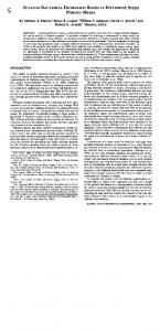
Figure 1: Transparent separation surfaces originating at stagnation points related to vortex breakdown on the delta wing (red and yellow). The blue stream surface originates at the tip of the wing and wraps the vortex core up to the breakdown point.

A BSTRACT In this paper, we present an approach for monitoring the positions of vector field singularities in time-dependent datasets. The concept of singularity index is discussed and extended from the well-understood planar case to the more intricate three-dimensional setting. Assuming a tetrahedral grid with linear interpolation in space and time, vector field singularities obey rules imposed by fundamental invariants (Poincar´e index), which we use as a basis for an efficient tracking algorithm. We apply the presented algorithm to CFD datasets to illustrate its purpose in the examination of structures that exhibit topological variations with time and describe some of the insight gained with this method. We give examples that show a correlation in the evolution of physical quantities that constitute to vortex breakdown. CR Categories: I.4.7 [Image Processing and Computer Vision]: Feature Measurement— [I.6.6]: Simulation And Modeling— Simulation Output Analysis J.2 [Physical Sciences and Engineering]: Engineering—. Keywords: flow visualization, topology tracking, time-dependent datasets, vortex breakdown

1

I NTRODUCTION

In the design of modern aircraft, computer simulations are an important tool in the development of new prototypes. While the basic

principles of aerodynamics have not changed much over the years, they are applicable to large scale problems only and do not describe the increasingly important details. The quality of numerical models has risen to a point where simulations can fill this gap. As the demand for faster aircraft and improved security is high, they have proven an extremely valuable tool in comparison to physical experiments. Aside from the validation of prototypes, simulations can help to increase our understanding of the dynamics of some of the more complex flow patterns that keep appearing in aviationrelated problems. They facilitate complicated flow experiments and provide accurate measurements not only at points of interest (that might not even be known a priori) but over the whole domain considered, and it is possible to evaluate quantities that cannot be measured physically. However, the advantage of complete data for a given problem is also a hindrance in its analysis. Since detailed models require fine resolutions, the amount of generated data is enormous. This is especially true for time-dependent problems. Resulting datasets are usually multi-gigabyte sized. Thus the problem of interpretation of a dataset often encompasses finding points of interest first. Concerning the design of delta-wing type aircraft, for both civil and military use, the vortex breakdown phenomenon has stood in the way of a wide application of these designs. The greater part of the lift a delta wing experiences is created by a system of vortices above the wing. This results in generally very good maneuverability and the possibility of high airspeeds. However, it can be observed that in certain situations (low speed and high angle of attack) these vortices tend to break down in the sense that the flow pattern becomes unstable and the vortical structure almost disappears, resulting in a loss of lift that can have fatal consequences regarding controllability of the aircraft. Furthermore, the pressure differences inherent in the breakdown can severely damage the structure of the aircraft. Therefore, there is a need to understand the origins of this phenomenon such that it can be avoided in future designs. While understanding is still incomplete, it is known that vortex breakdown is character-

ized by the appearance of stagnation points on the axis of the primary vortices[8]. Here, numerical simulations can show their full power by providing insight that will help the development of theories as to why and when vortex breakdown will occur. Although the phenomenon can be reproduced in stationary simulations, the full dynamics are only available from time-dependent calculations. Figure 1 depicts a sequence of vortex breakdowns from such a simulation. To obtain insight from resulting datasets we have developed an algorithm to detect and track the stagnation points (which are essentially zeros of the velocity field) over time and discover the relations between them (i.e. the structural evolution of the vector field) and characteristics of related quantities such as acceleration and helicity. The algorithm was developed to work on three-dimensional unstructured tetrahedral grids, since this is the form the datasets usually take. A visualization of the results (four dimensional in nature and thus hard to present) is then given by reducing the problem to two dimensions. To keep the algorithm simple and efficient, we have drawn on the theory of dynamical systems, namely the theory of the Poincar´e index. The main statement here is that vector field singularities in piecewise linear fields obey a set of rules that simplify their tracking through time. The work shown here is related to the usual notion of flow topology; however, we are not concerned with extracting all topological elements but rather a suitable small subset of its temporal evolution. The paper is structured as follows: Section 2 gives an overview over previous and related work. In Section 3, we detail some theoretical results related to the Poincar´e index, with a special emphasis on three-dimensional problems. Subsequently, the tracking algorithm is developed in Section 4, before we write about some issues related to preprocessing of the datasets and post-processing of the results in Section 5. The results we obtained from applying our algorithm to actual datasets are given in Section 6 before we conclude on the work shown here in Section 7.

2

R ELATED W ORK

The appearance of vortex breakdown (some authors call it vortex burst) has concerned many authors in the fluid mechanics community due to its relevance for a number of applications (see e.g. [8]). In the field of visualization, Kenwright and Haimes[6] were among few to write about the detection and visualization of vortex breakdown. They already emphasize its importance in aeronautics. Their interpretation of vortex breakdown is a significant change in the direction of the vortex core. From today’s point of view, this explanation is slightly misleading, since the role of flow singularities and their effect on vortex core detection methods was not understood. Concerning the temporal variation of features, there are approaches that detect features in several timesteps and perform a matching procedure to extract their evolution (e.g. Silver and Wang[10] and Samtaney et al.[9]). Making explicit use of the temporal interpolation, Weigle and Banks[13] extract features in the form of fourdimensional isosurfaces. A similar course is followed by Bauer and Peikert[1]. They incorporate a scale-space approach into their method for the tracking of vortex cores. As to the interrelations among multiple features over time, Silver et. al[2] have developed the feature tree that is related to the structural graph we establish in Section 5. The importance of singularities and separatrices in flow fields was recognized quite early by Helman and Hesselink[4] and resulted in two-dimensional topology visualization. Complete threedimensional topology has not been attempted yet, however there are

authors that examine suitable subsets, such as Theisel et. al[11]. In their paper, they compute saddle connectors as a basis for a topological skeleton. Relaxing the meaning of separation surfaces, Mahrous et al.[7] recently published a method for topological segmentation of steady vector fields surfaces that separate flow regions with different properties. Tricoche et al.[12] describe how the time-tracking of singularities and the corresponding topological variations can be investigated for 2D vector fields. This paper essentially extends their method to three spatial dimensions, however, we concentrate on the critical points and do not treat topology. 3

T HE P OINCAR E´ I NDEX IN 3D

Remark: In the following, when we speak of singularity, we will mean isolated zeros of a vector field. In two dimensions, the index concept is well understood and has been explained by several authors (see e.g. [12]). We immediately start in a three-dimensional setting: let v(x) a three-dimensional smooth vector field. We employ the notion of closed surfaces, i.e. surfaces that are topologically equivalent to a sphere. The basic idea of the index is the answer to the question of how many times a vector field “rotates” in the neighborhood of a point. Rotations in 3D are not easily measured and compared (we would need to employ quaternions), therefore, we take a slightly different and more geometric approach. We introduce the winding number #x (S) of a closed surface S with respect to a point x: 1 4π

#x (S) :=

y−x dS(y). |y − x|3

Z

S

The winding number can be proven to be integer and can be interpreted as the number of times S wraps around x. For example, the x-centered unit sphere has the canonical winding number 1. Now, to define the index of a closed surface S, we apply a simple notion: first, we introduce the Gauss map

γ : R3 \{0} → S2 , x 7→

x , ||x||

that maps any non-zero vector to its direction. The index k of a closed surface S is then defined as the number of times the vector field directions on S cover the origin as we move around all of S. In other words, it is the winding number of the Gauss map of v restricted to S with respect to the origin. Mathematically speaking, we have 4π k = #0 (γ (v|S )) =

Z

S

γ (v(x))dS(γ (v(x))).

(1)

Note that the winding number can be read as an oriented (“directed”) area integral of γ (v|S ) (cf. [5]). Hence, the sign of k depends on the orientation of S relative to R3 . We are able to define indz (v) of a singularity z via indz (v) := lim #0 (γ (v|Bε (z) )). ε →0

(2)

Furthermore, we find a very useful result: let S a closed surface that encloses the vector field singularities zi . Then

∑ indz (v) i

= #0 (γ (v|S )).

i

As a consequence of the last equation, we are able to calculate the index of a singularity by enclosing it with a surface small enough

While it seems that (3) is easily applied to piecewise linear vector fields, evaluation of the determinant is numerically unstable. If |detJ| is very small, rounding errors can easily cause a change of sign and therefore lead to a wrong result. We next present a more geometric approach that does not suffer these instabilities.

−−γ−→

3.2

Linear interpolation over tetrahedra

Datasets from applications are usually based on unstructured grids with cell-based linear or trilinear interpolation. We briefly show how index computation can be achieved on a piecewise linear tetrahedral grid. Let v(x) a linear vector field. Let T a tetrahedron with vertices pi , i = 0 . . . 3. T is positively oriented in the sense that the points are numbered in such a way that all face normals point outside. Let vi the vector values of v at the points pi . Since v is linear, it coincides with the barycentric linear interpolant of the vi on T :

−−γ−→

3

v(x) = Figure 2: Vector field directions on a closed surface S. Upper row: the directions do not cover S2 , hence the winding number of γ (v|S ) is zero. Lower row: S2 is covered once, |#0 (γ (v|S ))| = 1.

not to contain any other singularities. Furthermore, the shape of the surface does not matter as long as orientation is fixed relative to R3 for all such surfaces. As in the two-dimensional case (where one usually considers positively oriented paths), we will assume positive orientation for all closed surfaces henceforth. As a special case of this last equation, we find that if the index of S vanishes, S does not enclose any singularity in its interior. Although this definition is appealing in the mathematical sense, its application for computing indices in e.g. piecewise linear vector fields as often presented by applications is tedious. We therefore proceed by looking for an easier means to determine a singularity’s index in these cases. 3.1

Linear vector fields

βi (x) vi ,

3

∑ βi (x)

= 1.

i=0

i=0

Hence, v restricted to T is again a tetrahedron, T˜ . By application of the Gauss map to T˜ , we find that the vi are mapped to points vˆi on S2 and that the image of faces of T˜ are spherical triangles Sl . The area covered by Sl is less than 2π in modulus (this is a consequence of the minimal variation property of linear interpolation). It remains to compute the winding number w.r.t. the origin of the resulting closed surface S consisting of the spherical triangles Sl . We can write in analogy to (1) (recall that the vˆi have modulus 1) #0 (S) =

1 4π

Z

3

xdS(x) =

S

∑ areasigned (Si )

i=0

For Si , we find the length of its sides to be a = 6 (vˆi , vˆ j ) b = 6 (vˆi , vˆk ) c = 6 (vˆ j , vˆk )

= = =

arccos(vˆi · vˆ j ) arccos(vˆi · vˆk ) arccos(vˆ j · vˆk )

With s = 21 (a + b + c), we obtain the formula

Consider a linear vector field of the form v(x) = Jx + c.

(3)

It is quite easy to see how this simple formula works: since J is one-to-one, we easily find that | indz (v)| = 1 (all directions on the unit ball are reached exactly once). Hence, the sign of the index only depends on the relative orientations of S and γ (v|S ) for any S that wraps z. If J is orientation-preserving (i.e. det(J) > 0), the index is +1, otherwise it is −1. Hence (3) holds. There is a simple connection between the usual classification of linear singularity types (e.g. saddle, node, etc.) and the index. The index is essentially the sign of the product of the eigenvalues of the Jacobian matrix at the singularity. Since in three-space, the Jacobian has three eigenvalues, this allows for a wider range of possibilities than in two dimensions. For example, in 2D a saddle point has always index −1, whereas in 3D in can have both +1 or −1. This shows that the geometry of the defining space has a strong influence on the geometry of vector fields and the nature of apparent vector field singularities.

r

s s−a s−b s−c tan tan tan . 2 2 2 2 (4) In conclusion, the index of T is computed by evaluation of the angles between the vi . This computation may seem complicated because a lot of trigonometric functions are involved. However, the result can be expected to be close to an integer, therefore we can employ rounding to guarantee an accurate result. areasigned (Sl ) = 4 ∗ arctan

If J has full rank, v has exactly one isolated singularity at z = −J −1 c. Then, the index of v at z is given by the sign of J, i.e. indz (v) = sign(det J).

∑

tan

−−γ−→

Figure 3: The Gauss map γ maps a tetrahedron face to a spherical triangle.

3.3

Time-dependent vector fields

Let v(x,t) a smooth time-dependent vector field, and let S(t) a closed surface that changes position and shape smoothly with time. Then, if v(x,t) 6= 0 ∀t, x ∈ S(t), (5) the index of S(t) is constant in t. Condition (5) essentially ensures that no singularity is passing through S(t) as time increases. Hence, the zi enclosed by S(t) will remain enclosed, and no other singularity can join them. The argument then proceeds along the same lines as earlier. The right hand side of (2) varies continuously with time, and at the same time, it is integer; hence it must remain constant. The significance of this statement is large: it basically states that the index of a closed surface S(t) is conserved over time, which allows us to impose certain restrictions on the temporal evolution of singularities enclosed in S(t). The most important one for our purposes is that singularities must appear or disappear in groups such that the sum of their indices vanish. For example, if a pair of singularities is created, they must have indices of +k and −k respectively. Such a change of the structure of a vector field with a parameter (in our case the parameter is time) is called a structural bifurcation. A more extensive treatment of the theory of bifurcations of vector fields can be found in the book by Guckenheimer and Holmes [3].

4

T RACKING OF SINGULARITIES

and one must be located in T1 and the other in T2 . Moreover, due to conservation of the index, the overall index must remain zero, hence the indices of the singularities must be +1 and −1. Hence, bifurcations on faces are of a relatively simple nature. It would now be in order to discuss bifurcations on edges or vertices. However, these cases are quite intricate. Since more than two tetrahedra are involved, the list of possible bifurcation types is long, and non-linear singularities can occur (cf. [3]). We are mainly concerned with application datasets that usually show some amount of numerical noise, making the occurrence of a bifurcation on an edge or on a vertex of the grid extremely unlikely at best. Therefore, we limit ourselves to the case of face bifurcations since it is of greatest relevance. 4.2

Paths in a Tetrahedron

We first consider a single tetrahedron T and determine what possibilities exist for the path of a singularity z. To simplify the notation, we assume that the vector field in T is given in the form 3

v(x) =

∑ βl (x) ((1 − t)ui + tvi )) ,

x ∈ T,t ∈ [0, 1]

i=0

and that v is non-degenerate, i.e. it contains exactly one isolated zero at all times. For fixed t we can solve for the position of the singularity of this field in barycentric coordinates. For example, with wi (t) = (1 − t)ui + tvi we write (omitting the parameters) v = w0 + β1 (w1 − w0 ) + β2 (w2 − w0 ) + β3 (w3 − w0 )

In the following we will be concerned with developing an algorithm to the purpose of determining the paths of isolated singularities of a time-dependent piecewise-linear vector field, given on a tetrahedral grid. j

Let pi ∈ R3 a set of points and vi the vector values associated with the pi at discrete times t j ∈ R. Let Tk a set of tetrahedra defined on the points pi . Then every tetrahedron Tk gives rise to a vector field v(x,t) that is linear in both space and time: if x ∈ Tk and t ∈ [t j ,t j j + 1], then set 3

v(x,t) =

∑ βl (x)

l=0

µ

t − t j j+1 t j+1 − t j v + v t j+1 − t j l t j+1 − t j l

¶

,

where βl are the barycentric coordinates w.r.t. Tk and l refers to the vertices of Tk . We will next examine the paths of singularities in a single tetrahedron Tk . 4.1

Bifurcations

Considering structural changes, we have determined that a tetrahedron can include at most one isolated singularity, because the field is linear. This has one major implication: structural bifurcations cannot occur in linear vector fields. For the case of piecewise linear fields this implies that bifurcations must be located in places where two linear pieces are adjacent. For tetrahedral grids with per-tetrahedron linear interpolation, we find that bifurcations must happen in places where the field is not linear, i.e. on the boundaries between different tetrahedra. There are three possibilities: vertices, edges and faces of the grid. We will consider faces first. Assume we have two tetrahedra T1 and T2 that share a common face on which we find a bifurcation at some time t. Since the field is linear in both tetrahedra, only two singularities can be involved

and apply Cramer’s rule to find

β1 (t) =

det(−w0 , w2 − w0 , w3 − w0 ) b (t) =: 1 . det(w1 − w0, w2 − w0, w3 − w0) q(t)

The same can be done for all βi . Brief computation shows that the resulting bi (t) and q(t) are polynomials of degree 3 in t. We required that v be non-degenerate, this reflects in q(t) 6= 0 for all t ∈ [0, 1]. Naturally, if βi (t) < 0 for some i, the singularity of v is outside the tetrahedron for this specific t. In other words, we have found an explicit representation for the location of z. Taking a closer look at bi , we find that the zeros of these polynomials allow us to determine when z crosses one of T ’s faces. If for tˆ ∈ [0, 1] we find βi (tˆ) = 0 and β j (tˆ) >= 0 for j 6= i, then the singularity is located on the face of T opposite the vertex pi (its barycentric coordinate is zero). Furthermore, by evaluating the sign of the derivative µ ¶0 b0 (tˆ) bi βi0 (tˆ) = (tˆ) = i q q(tˆ) we can tell if the singularity enters or leaves the tetrahedron at tˆ and through which face. We will say that T has an entrance/exit on face F at tˆ. This information is important to determine in which neighboring tetrahedron (if one exists for F) the singularity path continues. For fixed t ∈ [0, 1] there can be at most one singularity inside T (since the field in T is linear), hence we can conclude that if there is a singularity in T at some t ∈ (0, 1), it must either have entered T at an earlier time 0 < tˆ < t or remained in T since t = 0 (in this case we will say that z enters at t = 0). In complete analogy, it must either exit T at t < t˜ < 1 or remain in T until t = 1 (read z exits at t = 1). In other words, a singularity path always connects an entrance to an exit, and exits and entrances always come in pairs. Since there cannot be more than one singularity in T at a given time, an entrance is always connected to the closest exit (w.r.t. t).

T1

4. for all bifurcations in B: check if B has two paths connecting to it; if it does not, there must be another singularity involved. Follow its path forward or backward in time depending on whether the bifurcation is a creation of singularities or an annihilation.

position

entrance exit entrance/exit

(a) the path must end at a bifurcation; add it to B; goto 4.

bifurcation

t j+1

t j+2

t j+3

time

Figure 4: Structural evolution of singularities. Three spatial dimensions are represented on the vertical axis.

When z passes from T to a neighbor T 0 through the face F at tˆ, in both T and T 0 there is a singularity on F at tˆ. There are two possibilities: either we find an exit/entry combination in T and T 0 , in which case the path continues in T 0 , or we find an exit/exit or entrance/entrance combination. In the last case, the vector field has a structural bifurcation on F at tˆ (i.e. creation or annihilation of a pair of singularities), and the paths of both singularities involved start or end on F.

4.3

Tracking algorithm

Having simplified matters so far, we now give a simple scheme for tracking a singularity path between two timesteps t = 0 and t = 1 that works by simply connecting entrance/exit path segments over tetrahedron boundaries. Assume that a singularity z is present in T at t ∈ (0, 1). Then, to compute the path forward in time 1. compute the bi and q for T , and determine entrances and exits 2. if there is no exit later than t, z exits T at t = 1; the path is complete 3. if there are exits in T , then z leaves T at the earliest exit later than t; determine the neighbor tetrahedron T 0 corresponding to the exit face F and compute b0i , q0 for T 0 4. if T 0 has an exit on F corresponding to the exit on T (→ bifurcation), the path of z ends on F 5. otherwise, T 0 has an entrance on F corresponding to the exit on T ; z is now in T 0 . Set T = T 0 and restart at 1. Following the path of z backwards in time can be achieved in a completely analogous manner. Both directions are completely equivalent. We use this procedure as a building block for computing the paths of all singularities present in two given timesteps between t = 0 and t = 1: 1. find the sets of tetrahedra S0 and S1 that contain a singularity at t = 0 and t = 1 respectively. Let B = {} the set of bifurcations encountered in between t = 0 and t = 1. 2. for every T ∈ S0 : follow the path of z forward in time (a) if it ends in T 0 at t = 1, eliminate T 0 from S1 . (b) if it ends at a bifurcation, add it to B. 3. for every T ∈ S1 (singularities not reached by paths from t = 0): follow the path of z backward in time (a) it must end at a bifurcation; add it to B

The algorithm essentially avoids multiple tracing of the same path by making use of the equivalence between forward and backward tracing (i.e. if a path extends from t = 0 to t = 1, we only need to trace it forward). The extra effort in step 4 is required because non-intuitive situations can occur (see Figure 5). The end result is a set of paths that completely describe the continuous structural variation of the vector field between the two timesteps. Going to several timesteps from here is easy as it only involves connecting the paths from different timesteps according to which singularity they start/end at. Remark: some cases are not covered by the given algorithm. For example: if the two bifurcations that create and annihilate a pair of singularities lie between two timesteps, neither of the singularities will show up in one of the timesteps, and hence their paths will not be discovered by the algorithm (see Figure 5). However, since they do not interact with other singularities, they do not play an important role in understanding the structural changes in between the timesteps. Moreover, it is often desirable to ignore small-scale local behavior (see also Section 5). 5 5.1

A PPLICATION TO DATASETS Pre- and post-processing

To obtain a complete picture of the structural evolution of a given dataset, the interaction of the various singularities form a structural graph with bifurcations as vertices and paths as edges (see Fig. 6 for an example). We will shortly describe how this graph can be used in post-processing of results. The method shown in Section 4 is limited to tetrahedra and the given dataset must be tetrahedrized before application. Although the tracking algorithm could be enhanced to deal with nontetrahedral grid cells, a generalization would result in a number of special cases that complicate the relatively simple structure of the algorithm. In the form presented above, implementation is straightforward and fast. However, a small price has to be paid: tetrahedrization of arbitrary grids can result in the creation of singularities that are not in the original dataset. It is possible that a cell of T2

entrance position

T0 tj

exit T1

entrance/exit bifurcation

T0 tj

t j+1 t j

t j+1

time

Figure 5: Left: Tracking only paths originating on timesteps does not completely explain the structural evolution (the blue path would not be discovered). Making sure that every bifurcation has two paths connecting to it solves this problem. Right: Paths that are not discovered since they have no entrance or exit on a timestep.

index 0 is split up in such a way that the resulting tetrahedra have non-vanishing index. These “artificial” singularities do not pose a problem, since they are always created in pairs and usually only last for a very brief amount of time. Numerical datasets are often subject to noise, especially if the computations involve some kind of differentiation. It is common practice to apply smoothing operators to datasets in order to undo some of the damage done by previous computations. Commonly, numerical noise reflects in short-lived pairs of artificial singularities that exist in isolation and are not part of the dataset’s structural evolution over time. It can also occur that a path is “interrupted” by a pair of artificial bifurcations that enclose a path segment of very short duration (Fig. 5 (left) gives an example). What seems a drawback at first can be turned into an advantage: instead of smoothing the dataset we filter the resulting set of singularity paths by removing paths that last less than e.g. one timestep. Filtering can be applied on the structural graph directly and can be implemented in an efficient way by first removing edges that represent paths with short duration and successively removing all isolated vertices. In our experiments, we found this method to be very effective in treating noisy datasets. It turns out that conventional smoothing does not significantly reduce the number of artificial singularities. It however affects the structure of the dataset in such a way that the structural evolution is obscured or changed (this is especially true for minimum/maximum tracking as described in the next paragraph).

5.2

Tracking of minima and maxima

which to describe the location of singularities. For more complicated datasets, higher order terms of the PCA and interpolation can be drawn upon to generate a curved coordinate. The resulting twodimensional diagrams quickly enable the viewer to discover key points in the structural evolution that can then be analyzed in detail with other methods.

6

R ESULTS

We have applied our algorithm to two different time-dependent datasets of CFD simulations performed by the German Aerospace Center (DLR)/G¨ottingen using their TAU code. All datasets take the form of a velocity field provided on the vertices of an unstructured grid consisting of tetrahedra, pyramids and prisms. Although the simulations are based on problems that show some degree of symmetry, the computation was performed on the full domain. While the can dataset retains the symmetry of the original problem, the delta wing dataset shows increasingly different behavior on both sides of the wing as time passes. It is already known that vortex breakdown is associated with the occurrence of (pairwise) stagnation points, therefore we have applied the tracking algorithm to the velocity fields first. Furthermore, there are speculations that both acceleration and helicity play an important role in this context. We have computed these fields for those datasets and applied tracking to them as well, in the case of helicity (which is a scalar quantity) minimum tracking was performed (as described in Section 5). Since these computations involved taking derivatives of the original velocity fields, we observed strong numerical noise in both helicity and acceleration yielding many artificial singularities. Using the structural graph filtering method described in Section 5 we were still able to obtain meaningful results.

The presented algorithm is concerned with tracking singularities in vector fields. By applying the above approach to gradient fields of scalar quantities, we are able to track the evolution of minima and maxima throughout time through following the paths of the associated singularities in the gradient fields. The algorithm can be directly applied to this modified problem. The resulting structural graph can then be filtered to only include paths of suitable singularities, i.e. attracting and repelling nodes. Note that while minima and maxima do not necessarily appear in pairs, they are still created and destroyed at bifurcations in the structural evolution. Although e.g. saddle points in the gradient field might have some physical meaning as well, we did not consider them in our examples (see Section 6).

The tracking algorithm itself is of linear complexity in both the number of singularities and the number of timesteps. The most time-intensive part is the pre-computation of all singularities in a timestep, for which each cell has to be considered individually. If this information is already given, the running times for our examples are on the order of seconds. Since the algorithm only needs two successive timesteps to do its work, it is possible to integrate it directly into the CFD simulation. The structural graph for all timesteps can then be completed in post-processing. This would also allow for online supervision of simulations that are still in progress. We will now detail the results for both datasets.

5.3

6.1

Visualization

The structural evolution of a vector field is basically a graph whose vertices have a total of four coordinates (3D space + 1D time). Representing the paths of singularities in three-space directly turns out to be non-intuitive, and adding temporal information to the presented locations via color-coding or animation does not help. Therefore, we approach the problem by first reducing the dimension from four to two by a change of coordinates. In one of our examples (cf. 6), the dataset is highly rotation symmetric and singularities appear and move on the symmetry axis only. Their complete evolution is then easily represented in a 2d diagram. However, the other example is much more intricate, and there is no canonical axis to represent the movement of the singularities. If the positions of all singularities at all times are taken into account, then we are able to determine the principal spatial direction and the common center of their movement by evaluating the zeroth and first order terms of the corresponding principal component analysis. This provides a suitable spatial coordinate along

Can dataset

The simulation describes a can filled with a highly viscous fluid that is accelerated by rotation of the lower lid. The rotational speed varies over time, leading to breakdown of the central vortex that covers the symmetry axis of the can. Due to the high viscosity of the fluid and the high degree of symmetry the velocity field is of very good numerical quality. This dataset is very close to being a standard model of vortex breakdown. It consists of about 5000 timesteps on a grid with approx. 4.4 million tetrahedra after decomposition. The results are of almost analytical quality (see Figure 6). The simulation actually shows two occurrences of vortex breakdown (and two corresponding pairs of stagnation points) and it is interesting to observe how primary and secondary vortex breakdown successively merge and re-split. Acceleration zeros and helicity minima show a strong correlation with the onset of the breakdown process and the bifurcation that creates the two stagnation points. Before our analysis of the dataset, this correlation was not known. It is also obvi-

ous that the structural graph serves as a kind of “directory” for the different timesteps by indicating interesting phenomena. Through this, relevant timesteps can be identified quickly and reliably.

6.2

Delta Wing dataset

In order to study vortex breakdown in aviation, an unsteady simulation of a delta wing configuration was performed. The angle of attack is increased over time, and the primary vortices eventually exhibit breakdown. The simulation totals 1000 time steps that describe the formation and breakdown of the primary vortices over time. The grid consists of about 18 million tetrahedra after decomposition. The dataset is somewhat noisy in a numerical sense since the resolution is still too low in some of the more interesting parts of the dataset (this is especially true for the vortex breakdown regions). Figure 7 provides an overview showing stream surfaces that wrap around the primary vortices above the wing (red and blue). Asymmetric breakdown is clearly visible. We have used our method on two regions in the dataset that correspond to breakdown on both sides of the wing. After the coordinate transformation (see also Section 5), the structural graph of the right region (cf. Figure 8) clearly shows the evolution of the stagnation points as they move towards the wing. Again, acceleration zeros and a helicity minimum seem to play a role in formation of breakdown, although the correlation is not as obvious as in the can dataset. This is, in part, to be blamed upon the lack in resolution and the resulting numerical instability of differentiation. Filtering of the structural graph for the helicity gradient field (whose computation involves a second spatial derivative) reduced the number of meaningful paths from roughly 1.000 to 4, effectively eliminating all artificial singularities. The left region is even more chaotic, and it is clearly visible how the stagnation points begin to oscillate and disappear around timestep 730, to be followed by what appears to be a sequence of short-lasting vortex breakdowns in different places. In this case, the structure graph helps in grouping the velocity field singularities that would otherwise just be isolated singularities in the field without any context. Figure 7 gives a direct comparison between the evolution of stagnation points on the left and right sides and the corresponding flow structures (displayed by stream surfaces). While the behavior is almost similar in the beginning, the left side quickly deteriorates. Again, the structure graph can provide for a direct qualitative comparison that is very hard to achieve by other means (e.g. streamlines or surfaces).

7

C ONCLUSION

The objective of the work presented in this paper was to determine the structural evolution of certain types of complex time-dependent CFD datasets. First, we have presented a number of theoretical results about the Poincar´e index in three spatial dimensions. It is an extremely powerful yet intuitively geometric concept of describing singularities of 3D vector fields and the laws they must obey under time-varying circumstances. Considering the restrictions imposed by tetrahedral grids with piecewise linear interpolation in space and time, we were able to give a robust and straightforward algorithm to the intended purpose. By providing a temporal overview of the dataset using the structural graph that is built from singularity paths, it is possible to quickly determine points of interest in large datasets with many timesteps. Furthermore, the method has already proven useful in the analysis of two datasets where the flow exhibits vortex breakdown. Since understanding of this phenomenon is still incomplete from a fluid mechanical point of view, we believe that

the uncovered interrelations of various quantities can be an important step towards a complete explanation. Here, visualization can show its strength by giving new impulses in fluid mechanics. There is however some space for improvement on the presented material. The tracking algorithm could be extended to deal with trilinear interpolation to make possible the treatment of CFD grids directly without the need for prior tetrahedrization. So far, singularities have not played a significant role in the analysis of CFD datasets; this has changed with the advent of simulations that are able to resolve very complex flow patterns. If a more complete picture of a given flow can be obtained via the structural graph, the detection of certain types of flow behavior could be automated based on the graph. With efforts underway to automatically optimize the geometries of e.g. aircraft to exclude undesired effects, the structural graph could provide a robust criterion to indicate their presence. Vortex breakdown serves as a prime example.

ACKNOWLEDGEMENTS Foremost, the authors would like to thank Markus Ru¨ tten from DLR G¨ottingen for close collaboration and insightful remarks. He kindly provided the datasets considered here. Our gratitude also extends to all members of the FAnToM project at the University of Kaiserslautern for their implementation efforts. This work was partly supported by DFG grants HA 1491/15-4 and HA 1491/15-5.

R EFERENCES [1] D. Bauer and R. Peikert. Vortex tracking in scale-space. In Data Visualization 2002. Proc. VisSym ’02, 2002. [2] J. Chen, D. Silver, and L. Jiang. The feature tree: Visualizing feature tracking in distributed amr datasets. In IEEE Symposium on Parallel and Large-Data Visualization and Graphics, 2003. [3] J. Guckenheimer and P. Holmes. Nonlinear Oscillations, Dynamical Systems, and Bifurcations of Vector Fields. Springer-Verlag, 1983. [4] J. L. Helman and L. Hesselink. Visualizing Vector Field Topology in Fluid Flows. IEEE Computer Graphics and Applications, 11(3):36– 46, May 1991. [5] D. Hestenes and G. Sobzyk. Clifford Algebra to Geometric Calculus. D. Reidel Publishing Company, 1984. [6] D. N. Kenwright and R. Haimes. Vortex Identification - Applications in Aerodynamics: A Case Study. In R. Yagel and H. Hagen, editors, IEEE Visualization ’97, pages 413–416, Los Alamitos, CA, 1997. [7] K. Mahrous, J. Bennet, G. Scheuermann, B. Hamann, and K. I. Joy. Topological segmentation in three-dimensional vector fields. IEEE Transactions on Visualization and Computer Graphics, 10(2):198– 205, 2004. [8] T. Mullin, J. J. Kobine, S. J. Tavener, and K. A. Cliffe. On the creation of stagnation points near straight and sloped walls. Physics of Fluids, 12(2), 2000. [9] R. Samtaney, D. Silver, N. Zabusky, and J. Cao. Visualizing features and tracking their evolution. IEEE Computer, 27(2):20 – 27, 1994. [10] D. Silver and X. Wang. Tracking and visualizing turbulent 3d features. IEEE Transactions on Visualization and Computer Graphics, 3(2), 1997. [11] H. Theisel, T. Weinkauf, H.-C. Hege, and H.-P. Seidel. Saddle connectors - an approach to visualizing the topological skeleton of complex 3d vector fields. In IEEE Visualization ’03, 2003. [12] X. Tricoche, T. Wischgoll, G. Scheuermann, and H. Hagen. Topology tracking for the visualization of time-dependent two-dimensional flows. Computers & Graphics, 26(2):249 – 257, 2002. [13] C. Weigle and D. C. Banks. Extracting iso-valued features in 4dimensional scalar fields. 1998.

4925

stagnation point helicity min. acceleration zero

timestep

2968

2458

1888 1602 secondary vortex breakdown

758

primary vortex breakdown

0

0.2

0.4 0.6 singularity position on principal axis

0.8

1

structural evolution

timestep 1700

timestep 4400

Figure 6: Left: Structural graph of the can dataset. The green paths represent the stagnation points in the velocity field. Primary and secondary breakdown each create a pair of stagnation points. Around timestep 1888, the two phenomena join, only to re-split at timestep 2458 and successively decay. The blue and orange paths belong to helicity minima and acceleration zeros. Note the strong interrelation between the three quantities. Right: Two snapshots from the can dataset. Separation stream surfaces are started at the singularity positions. Timestep 1700 shows both breakdowns, whereas the second breakdown has already vanished in timestep 4000 and the first breakdown shows the typical “mushroom” structure.

timestep

timestep

723

597

595 stagnation points helicity min. acceleration zeros 1

stagnation points helicity min. acceleration zeros 1.5

singularity position

right breakdown

1

1.5 singularity position

left breakdown

Figure 7: Left: Overview of the delta wing dataset with its two primary vortices above the wings. Stream surfaces wrap around the vortices and are eventually distorted by vortex breakdown. Note the asymmetrical breakdown structure. Right: Structural graphs for right and left breakdown. Again a connection between various quantities involved in vortex breakdown can be observed for the right breakdown. In the left breakdown, several oscillating breakdown structures are visible in the later timesteps.

860

timestep

780

700

620

stagnation points left stagnation points right 540

1

1.5 singularity position

structural evolution left vs. right

timestep 730 (right vortex breakdown)

timestep 730 (left vortex breakdown)

Figure 8: Comparison of right and left breakdown structures. Left: The combined structural graphs make an intuitive comparison possible. Right: transparent stream surfaces show the distortion of the flow and the intricate flow patterns that make analysis difficult. The left breakdown does not show the usual breakdown structure and consists of several smaller and independent breakdowns.