Trading classical and quantum computational resources

Trading classical and quantum computational resources Sergey Bravyi, Graeme Smith, and John A. Smolin

arXiv:1506.01396v1 [quant-ph] 3 Jun 2015

IBM T.J. Watson Research Center, 1101 Kitchawan Road, Yorktown Heights, NY 10598 We propose examples of a hybrid quantum-classical simulation where a classical computer assisted by a small quantum processor can efficiently simulate a larger quantum system. First we consider sparse quantum circuits such that each qubit participates in O(1) two-qubit gates. It is shown that any sparse circuit on n + k qubits can be simulated by sparse circuits on n qubits and a classical processing that takes time 2O(k) poly(n). Secondly, we study Pauli-based computation (PBC) where allowed operations are non-destructive eigenvalue measurements of n-qubit Pauli operators. The computation begins by initializing each qubit in the so-called magic state. This model is known to be equivalent to the universal quantum computer. We show that any PBC on n + k qubits can be simulated by PBCs on n qubits and a classical processing that takes time 2O(k) poly(n). Finally, we propose a purely classical algorithm that can simulate a PBC on n qubits in a time 2αn poly(n) where α ≈ 0.94. This improves upon the brute-force simulation method which takes time 2n poly(n). Our algorithm exploits the fact that n-fold tensor products of magic states admit a low-rank decomposition into n-qubit stabilizer states.

I.

INTRODUCTION

Quantum computers promise a substantial speedup over classical ones for certain number-theoretic problems and the simulation of quantum systems [1–3]. Experimental efforts to build a quantum computer remain in their infancy though, limited to proof-ofprinciple experiments on a handful of qubits. In contrast, the design of classical computers is a mature field offering billions of operations per second in offthe-shelf machines and petaflops in leading supercomputers. To prove their worth, quantum computers will have to offer computational solutions that rival the performance of classical supercomputers, a daunting task to be sure. Here we study hybrid quantum-classical computation, wherein a small quantum processor is combined with a large-scale classical computer to jointly solve a computational task. To motivate this problem, imagine that a client can access a quantum computer with 100 qubits and essentially perfect quantum gates. Such a computer lies in the regime where it is likely to outperform any classical machine (since it would be nearly impossible to emulate classically). Imagine further that the client wants to implement a quantum algorithm on 101 qubits, but it is impossible to expand the hardware to accommodate one extra qubit. Does the client have any advantage at all from the access to a quantum computer in this scenario? Can one divide a quantum algorithm into subroutines that require less qubits than the entire algorithm? Can one implement each subroutine separately and combine their outputs on a classical computer? These are the main questions addressed in the present paper. Put differently, we ask how to add one virtual qubit to an existing quantum machine at the cost of an increased classical and quantum running times, but without modifying the machine hardware. More generally, one may ask what is the cost of adding k virtual

qubits to an existing quantum computer of n qubits and how to characterize the tradeoff between quantum and classical resources in these settings. As one may expect, the cost of adding virtual qubits varies for different computational models. Although the circuit-based model of a quantum computer is the most natural and well-studied, several alternative models have been proposed, such as the measurementbased [4] and the adiabatic [5] quantum computing, as well as the model DQC1 where most of the qubits are initialized in the maximally mixed state [6]. Our goal is to identify quantum computing models which enable efficient addition of virtual qubits. Below we describe two examples of such models. We begin with the model based on sparse quantum circuits. Recall that a quantum circuit on n qubits is a collection of gates, drawn from some fixed (usually universal) gate set, with n input qubits and n output qubits. Below we assume that the gate set includes only one-qubit and two-qubit gates. Let us say that a circuit is d-sparse if each qubit participates in at most d two-qubit gates. We shall be interested in the regime when d is a constant independent of n or when d grows very slowly, say d ∼ log (n). This regime covers interesting quantum algorithms that can be described by low-depth circuits [7] since any depth-d quantum circuit must be d-sparse (although the converse is generally not true). It is believed that a constant-depth quantum computation cannot be efficiently simulated by classical means only [8, 9]. It is also likely that early applications of quantum computers will be based on relatively low-depth circuits because they impose less stringent requirements on the qubit coherence times. Define a d-sparse quantum computation, or d-SQC, as a sequence of the following steps: (i) initialization of n qubits in the |0i state, (ii) action of a d-sparse quantum circuit, (iii) measurement of each qubit in the 0, 1 basis, and (iv) classical processing of the measurement outcomes that returns a single output bit

2 bout . We require that the final classical processing takes time at most poly(n). A classical or quantum algorithm is said to simulate a d-SQC if it computes probability of the output bout = 1 with a small additive error. Our first result is the following theorem, which quantifies the cost of adding k virtual qubits to a d-SQC on n qubits. Theorem 1. Suppose n ≥ kd + 1. Then any d-sparse quantum computation on n+k qubits can be simulated by a (d + 3)-sparse quantum computation on n qubits repeated 2O(kd) times and a classical processing which takes time 2O(kd) poly(n). The above result is most useful when both k and d are small, for example, k = O(1) and d = O(log n). In this case both quantum and classical running time of the simulation scale as poly(n). On the other hand, we expect that a direct simulation of a d-SQC on a classical computer takes a super-polynomial time (see the discussion above). Hence the theorem provides an example when a hybrid quantum-classical simulation is more efficient than a classical simulation alone. The proof of the theorem exploits the fact that any d-sparse quantum circuit U acting on a bipartite system AB with |A| ≈ k and |B| ≈ n can be decomposed into a linear combination of 2O(kd) tensor product terms Vα ⊗ Wα , where Vα and Wα are d-sparse circuits acting on A and B respectively. We show that the task of simulating U can be reduced to simulating the smaller circuits Wα , as well as computing certain interference terms that involve pairs of circuits Wα , Wβ . We show that the interference terms can be estimated by a simple SWAP test which can be realized by a (d + 3)-sparse computation on n qubits. Our second model is called Pauli-based computation (PBC). We begin with a formal definition of the model. Let P n be the set of all hermitian Pauli operators on n qubits, that is, n-fold tensor products of single-qubit Pauli operators I, X, Y, Z with the overall phase factor ±1. A PBC on n qubits is defined as a sequence of elementary steps labeled by integers t = 1, . . . , n where at each step t one performs a nondestructive eigenvalue measurement of some Pauli operator Pt ∈ P n . Let σt be the measured eigenvalue of Pt . Note that σt = ±1 since any element of P n squares to one. We allow the choice of Pt to be adaptive, that is, Pt may depend on all previously measured eigenvalues σ1 , . . . , σt−1 . The latter have to be stored in a classical memory. The computation begins by initializing each qubit in the so-called magic state |Hi = cos (π/8)|0i + sin (π/8)|1i. Once all Pauli operators P1 , . . . , Pn have been measured, the final quantum state is discarded and one is left with a list of measured eigenvalues σ1 , . . . , σn . The outcome of a PBC is a single classical bit bout obtained by performing a classical processing of the measured eigenvalues. All classical processing must take

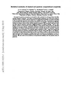
time at most poly(n). We shall prove that the computational power of a PBC does not change if one additionally requires that all Pauli operators P1 , . . . , Pn pairwise commute (for all measurement outcomes). A classical or quantum algorithm is said to simulate a PBC if it computes probability of the output bout = 1 with a small additive error. An example of a PBC is shown at Fig. 1. The PBC model naturally appears in fault-tolerant quantum computing schemes based on error correcting codes of stabilizer type [10]. Such codes enable a simple fault-tolerant implementation of non-destructive Pauli measurements on encoded qubits, for example using the Steane method [11]. Furthermore, topological quantum codes such as the surface code enable a direct measurement of certain logical Pauli operators by measuring a properly chosen subset of physical qubits [12]. Several fault-tolerant protocols for preparing encoded magic states such as |Hi have been developed [13–17]. PBCs implicitly appeared in the previous work on quantum fault-tolerance. Our analysis closely follows the work by Campbell and Brown [18] who showed that a certain class of magic state distillation protocols can be implemented by PBCs. Let us now state our results. First, we claim that a PBC has the same computational power as the standard circuit-based quantum computing model. Theorem 2. Any quantum computation in the circuit-based model with n qubits and poly(n) gates drawn from the Clifford+T set can be simulated by a PBC on m qubits, where m is the number of T gates, and poly(n) classical processing. Recall that the Clifford+T gate set consists of single-qubit gates       1 1 0 1 1 1 0 H=√ , S= , T = , 0 i 0 eiπ/4 2 1 −1 and the two-qubit CNOT gate. This gate set is known to be universal for quantum computing. Secondly, we show that PBCs enable efficient addition of virtual qubits. Theorem 3. A PBC on n + k qubits can be simulated by a PBC on n qubits repeated 2O(k) times and a classical processing which takes time 2O(k) poly(n). Both theorems follow from the fact that a generalized PBC that incorporates unitary Clifford gates, ancillary stabilizer states (such as |0i or |+i), and has poly(n) measurements can be efficiently simulated by the standard PBC defined above. To prove Theorem 2 we convert a given quantum circuit on n qubits with m T -gates into a generalized PBC on n + m qubits initialized in the |0⊗n i ⊗ |H ⊗m i state. Each T -gate of the circuit is converted into a simple gadget that includes adaptive Pauli measurements and consumes

3 one copy of the |Hi state. Simulating such generalized PBC by the standard PBC on m qubits proves Theorem 2. To prove Theorem 3 we represent k copies of the magic state |Hi as a linear combinationP of k-qubit stabilizer states φα such that |HihH|⊗k = α cα |φα ihφα | for some real coefficients cα . The number of terms in this sum is 2O(k) . We carry out the simulation independently for each α using a generalized PBC on k +n qubits initialized in the state |φα i ⊗ |H ⊗n i and combine the outcomes on a classical computer. Finally, we simulate the generalized PBCs by the standard PBCs on n qubits. Perhaps more surprisingly, we prove that PBCs can be simulated on a classical computer alone more efficiently than one could expect naively. Let us first describe a brute-force simulation method based on the matrix-vector multiplication. Let φt be the nqubit state obtained after measuring the Pauli operators P1 , . . . , Pt . One can store φt in a classical memory as a complex vector of size 2n . Each step of a PBC involves a transformation φt → φt+1 where φt+1 = (1/2)(I +σt Pt )φt . Since Pt is a Pauli operator, the matrix of Pt in the standard basis is a permutation matrix modulo phase factors. Thus, for a fixed vector φt , one can compute φt+1 for both choices of σt in time O(2n ). Furthermore, one can compute the norm of φt+1 in time O(2n ) and thus determine the probability of each measurement outcome σt . By flipping a classical coin one can generate a random variable σt = ±1 with the desired probability distribution. Since any PBC has at most n steps, the overall cost of the classical simulation is O(n2n ). Below we show that this brute force simulation method is not optimal. Theorem 4. Any PBC on n qubits can be simulated classically in time 2αn poly(n), where α ≈ 0.94. Our simulation algorithm exploits the fact that tensor products of magic states admit a low-rank decomposition into stabilizer states. Recall that an n-qubit state φ is called a stabilizer state if |φi = U |0⊗n i for some n-qubit Clifford operator U — a product of the elementary gates H, S, and the CNOT. Suppose ψ is an arbitrary n-qubit state. Define a stabilizer rank of ψ as the smallest Pχ integer χ such that ψ can be written as |ψi = α=1 cα |φα i, where cα are complex coefficients and φα are n-qubit stabilizer states. The stabilizer rank of ψ will be denoted χ(ψ). By definition, 1 ≤ χ(ψ) ≤ 2n for any n-qubit state ψ and χ(ψ) = 1 iff ψ is a stabilizer state. For example, the magic state |Hi has stabilizer rank χ(H) = 2, since |Hi is not a stabilizer state itself, but it can be written as a linear combination of two stabilizer states |0i and |1i. Furthermore, using the identity |H ⊗2 i =

1 1 (|00i + |11i) + √ (|00i + |01i + |10i − |11i) 2 2 2

one can easily check that χ(H ⊗2 ) = 2. More generally, let χn be the stabilizer rank of |H ⊗n i. Note that χn+m ≤ χn χm since a tensor product of two stabilizer states is a stabilizer state. In particular, χn ≤ (χ2 )n/2 = 2n/2 . The probability to observe measurement outcomes σ1 , . . . , σt in a PBC implemented up to a step t can be written as χn X hH ⊗n |Π|H ⊗n i = cα cβ hφα |Π|φβ i α,β=1

where φα are n-qubit stabilizer states, cα are complex Qt coefficients, and Π = a=1 (I + σa Pa )/2 is the projector describing the partially implemented PBC. We will use a version of the Gottesman-Knill theorem [19] to show that each term hφα |Π|φβ i can be computed on a classical computer in time n3 . Since the number of terms is χ2n and the number of steps is at most n, we would be able to simulate a PBC on n qubits classically in time (χn )2 n4 . Improving upon the bruteforce simulation method thus requires an upper bound χn ≤ 2βn for some β < 1/2. We establish such an upper bound with β = log2 (7)/6 ≈ 0.468 by showing that χ6 ≤ 7 which implies χn ≤ (χ6 )n/6 ≤ 7n/6 . We expect that the scaling in Theorem 4 can be improved by computing χn for larger values of n. In Appendix B we describe a heuristic algorithm for computing lowrank decompositions of |H ⊗n i into stabilizer states which yields the following upper bounds: n 2 3 4 5 6 χn ≤ 2 3 4 6 7 We believe that these upper bounds are tight. A lower bound χn ≥ Ω(n1/2 ) is proved in Appendix C. II.

DISCUSSION AND PREVIOUS WORK

Classical algorithms for simulation of quantum circuits based on the stabilizer formalism have a long history. Notably, Aaronson and Gottesman [19] studied adaptive quantum circuits that contain only a few non-Clifford gates. Assuming that a circuit contains at most m non-Clifford gates and that all n qubits are initially prepared in some stabilizer state, Ref. [19] showed how to simulate such a circuit classically in time 24m poly(n). To enable a comparison with our results, assume that all unitary gates belong to the Clifford+T set. By Theorem 2, a quantum circuit as above can be transformed into a PBC on m qubits, where m is the number of T -gates. Thus Theorems 2,4 provide a classical simulation algorithm with a running time 20.94m poly(n) which improves upon [19]. In addition, Ref. [19] studied adaptive quantum circuits composed only of Clifford gates and Pauli measurements with more general initial states. Assuming that the initial n-qubit state can be written as

4

_ _

+

_

_

+

+

_

+

_

+ +

_

+

FIG. 1. Example of a PBC on n = 3 qubits. Each step t involves an eigenvalue measurement of a Pauli operator Pt on n qubits with an outcome σt = ±1. A choice of Pt may depend on the outcomes of all previous measurements. A PBC on n qubits can be described by a binary tree T of height n such that internal nodes of T are labeled by n-qubit Pauli operators and leaves of T are labeled by 0 and 1. The latter represent the final output bit bout . We require that label of any node of T can be computed classically in time poly(n).

a tensor product of some b-qubit states, a quantum circuit as above can be simulated classically in time 22b+2d poly(n), where d is the total number of measurements [19]. Methods for decomposing arbitrary states into a linear combination of stabilizer states aimed at simulation of quantum circuits were pioneered by Garcia, Markov, and Cross [20, 21] who studied decompositions into pairwise orthogonal stabilizer states (named stabilizer frames). The latter are more restrictive than the general decompositions analyzed in the present paper. Furthermore, Refs. [20, 21] have not studied stabilizer decompositions of magic states. The simulation algorithm of Theorem 4 is conceptually close to the matrix multiplication algorithms based on tensor decompositions [22, 23]. In this case the analogue of a stabilizer state is a product state and the analogue of a magic state is a tripartite entangled state that contains EPR-type states shared between each pair of parties, see [24] for details. Efficient classical algorithms for simulation of quantum circuits in which the initial state can be described by a discrete Wigner function taking non-negative values were investigated by Veitch et al [25] and by Howard [26] et al. As was pointed out by Pashayan, Wallman, and Bartlett [27], such methods can be combined with Monte Carlo sampling techniques to enable classical simulation of general quantum circuits with the running time scaling exponentially with the quantity related to the negativity of the Wigner function. To enable a comparison between Theorem 4 and the

results of [27] one can employ a discrete Wigner function representation of stabilizer states and Clifford operations on qubits developed by Delfosse et al [28]. The latter is applicable only to states with real amplitudes and to Clifford operations that do not mix X-type and Z-type Pauli operators (CSS-preserving operations). A preliminary analysis shows that combining the results of Refs. [27, 28] yields a classical algorithm for simulating a restricted class of PBC on n qubits in time M 2n poly(n) ≈ 20.543n poly(n), where M = 2−1 + 2−1/2 ≈ 1.207 is the so-called mana of the magic state |HihH|, see [27, 28] for details. The restriction is that all Pauli operators to be measured are either X-type or Z-type, and the measurements cannot be adaptive. Such restricted PBCs are not known to be universal for quantum computation. Our method of simulating sparse quantum circuits has connections to ideas of tensor network representations of quantum circuits developed by Markov and Shi [29]. Indeed, our proof of Theorem 1 can be interpreted as a particular method of expressing the acceptance probability of a quantum computation in terms of a contraction of tensors associated with the quantum circuit. The individual entries of the tensors are then estimated separately with a smaller quantum computer and then added together. Let us now discuss some open problems and possible generalizations of our work. A natural question is whether the scaling in Theorem 4 can be improved if |Hi is replaced by some other magic state. By definition, any magic state is Clifford-equivalent to one of the states |Hi and |Ri, where |Ri√is the +1 eigenvector of an operator (X + Y + Z)/ 3, see Ref. [13] for details. The numerics suggests that |H ⊗n i and |R⊗n i have the same stabilizer rank for n ≤ 6. We conjecture that this remains true for all n. Moreover, we pose the following conjecture which, if true, highlights a new optimality property of magic states in terms of their stabilizer rank. Conjecture 1. Let χn be the stabilizer rank of |H ⊗n i and φ be an arbitrary single-qubit state. Then χ(φ⊗n ) = 1

if φ is a stabilizer state,

χ(φ

⊗n

) = χn

if φ is a magic state,

χ(φ

⊗n

) > χn

otherwise.

Less formally, the conjecture says that magic states have the smallest possible stabilizer rank among all non-stabilizer single-qubit states. It is also of great interest to understand the asymptotic scaling of the stabilizer rank χn . Assuming that a universal quantum computation cannot be simulated classically in polynomial time, one infers that χn must grow super-polynomially in the limit n → ∞. However, we were unable to derive such a lower bound directly without using any assumptions. The fact that

5 amplitudes of any stabilizer state in the standard basis take only O(1) different values implies a weaker lower bound χn ≥ Ω(n1/2 ), see Appendix C. We conjecture that in fact χn ≥ 2Ω(n) . Note that if this conjecture is false, that is, χn ≤ 2o(n) , then constantdepth circuits in the Clifford+T basis can be simulated classically in a sub-exponential time, which appears unlikely. Indeed, since such a circuit contains at most m = O(n) T -gates, where n is the number of qubits, Theorems 2,4 would provide a simulation algorithm with a running time χ2m ·poly(n) = 2o(n) poly(n). (Here we ignore the complexity of finding the optimal stabilizer decomposition since it has to be done only once for each n.) Finally, one may explore generalizations of the stabilizer rank to approximate decompositions into stabilizer states. It should be pointed out that the simulation algorithm of Theorem 4 would require approximate stabilizer decompositions with a precision at least 2−Ω(n) since the probability of a particular measurement outcome σ1 , . . . , σt can be exponentially small in n. It is not clear whether such approximate decompositions would have a rank substantially smaller than the exact ones. In the rest of the paper we prove the theorems stated in the introduction. From the technical perspective, Theorems 1,2,3 follow easily from the definitions and from the previously known results. On the other hand, Theorem 4 and the notion of a stabilizer rank appear to be new. We analyze sparse quantum circuits in Section III. A classical algorithm for simulation of PBCs and the stabilizer rank of magic states are discussed in Section IV. Theorems 2,3 are proved in Section V. Appendix A proves a technical lemma needed to compute inner products between stabilizer states. Appendix B describes a numerical method of computing low-rank stabilizer decompositions. Appendix C proves a lower bound on the stabilizer rank of magic states.

III.

|A| = k and |B| = n. Then U=

χ X

χ ≡ 24kd ,

cα Vα ⊗ Wα ,

(1)

α=1

where Vα and Wα are d-sparse quantum circuit acting on A and B respectively, Pχ and cα are some complex coefficients such that α=1 |cα |2 = 1. Proof. Since U is a d-sparse circuit, it contains at most kd two-qubit gates that couple some qubit of A and some qubit of B. Let G1 , . . . , Gm be the list of all such gates, where m ≤ kd. Any two-qubit gate G[i, j] acting on qubits i ∈ A and jP∈ B can be expanded in the 16 Pauli basis as G[i, j] = α=1 cα Pα [i] ⊗ Pα [j], where Pα ∈ {I, X, Y, Z} are Pauli operators and cα are some P complex coefficients such that α |cα |2 = 1. Applying the above decomposition to each gate G1 , . . . , Gm and, if necessary, appending dummy identity gates to make m = kd, one arrives at Eq. (1). Note that replacing a two-qubit gate in U by a tensor product of two single-qubit Pauli gates cannot increase the sparsity of the circuit. Thus each term Vα ⊗Wα is a tensor product of two d-sparse circuits. The classical post-processing step can be described by a poly(n) classical circuit f : Σn+k → {0, 1}. By definition of the SQC model, the final output of a computation is a single random bit bout = f (x), where x ∈ Σn+k is the bit string obtained by measuring each qubit of a state U |0n+k i in the 0, 1 basis. Let π(U ) be the probability of the output bout = 1, that is, π(U ) = h0n+k |U † ΠU |0n+k i, X

Π=

|xihx|.

(2)

x : f (x)=1

Let us first show how to estimate the quantity π(U ) with a small additive error using dk-sparse circuits on n + 1 qubits. Substituting Eq. (1) into the definition of π(U ) one gets

SPARSE QUANTUM CIRCUITS

π(U ) =

χ X X

cα (y)cβ (y)hφα |Π(y)|φβ i,

(3)

y∈Σk α,β=1

In this section we prove Theorem 1. All quantum circuits considered below are defined with respect to some fixed basis of gates G. We assume that any gate in G acts on at most two qubits. Furthermore, we assume that G contains all single-qubit Pauli gates X, Y, Z, their controlled versions, the Hadamard gate, and the π/2 phase shift S = |0ih0|+i|1ih1|. For example, G could be the Clifford+T basis. Let Σn ≡ {0, 1}n be the set of n-bit binary strings. Lemma 1. Let U be a d-sparse quantum circuit on k + n qubits. Partition the set of qubits as AB, where

where cα (y) = cα hy|Vα |0k i,

|φα i = Wα |0n i,

and Π(y) =

X

|zihz|.

z∈Σn f (yz)=1

We claim that each coefficient cα (y) can be computed exactly in time O(kd · 2k ). Indeed, we can merge consecutive single-qubit gates of Vα such that each qubit

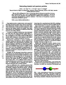
6 is acted upon by at most d two-qubit gates and at most d + 1 single-qubit gates. Thus we can assume that the total number of gates in Vα is O(kd). One can compute the quantity hy|Vα |0k i classically in time O(kd · 2k ) by performing matrix-vector multiplication for each gate of Vα . Furthermore, it is clear from the proof of Lemma 1 that each coefficient cα can be computed in time O(kd). Consider some fixed triple (y, α, β) that appears in the sum Eq. (3). Define a controlled-W operator Λ(W ) = |0ih0| ⊗ Wα + |1ih1| ⊗ Wβ . Define a quantum circuit R acting on n+1 qubits that consists of the following steps: (i) initialize n+1 qubits in the |0i state, (ii) apply H gate to the first qubit, (iii) apply Λ(W ) with the first qubit acting as the control one, (iv) apply H gate to the first qubit, (v) measure each qubit in the 0, 1-basis. The construction of R, illustrated at Fig. 2, is very similar to the standard SWAP test, except that we finally measure each qubit. Let b, z be the measurement outcomes, where b = 0, 1 and z ∈ Σn , see Fig. 2. Define a random variable 0 0 σy,α,β taking values ±1 such that σy,α,β = 1 iff b = 0 0 and f (yz) = 1. Otherwise σy,α,β = −1. A simple algebra shows that 0 Re(hφα |Π(y)|φβ i) = E(σy,α,β ),

(4)

0 is an unbiased estimator of the real part that is σy,α,β of hφα |Π(y)|φβ i. We claim that one can get a sample 0 of σy,α,β by executing a single instance of a dk-sparse quantum computation on n + 1 qubits (with certain special properties). Indeed, by construction, the circuits Wα and Wβ can be obtained from each other by changing some subset of at most kd single-qubit Pauli gates. Thus the controlled circuit Λ(W ) only needs control for at most kd single-qubit Pauli gates. This shows that the control qubit participates in at most kd two-qubit gates. Furthermore, since all locations where Wα and Wβ differ from each other originate from two-qubit gates in the initial d-sparse circuit U , we conclude that the circuit R has a special property that all qubits except for the control one participate in at most d two-qubit gates. One can similarly define 00 a random variable σy,α,β such that

that P is, π(U ) = E(ξ). Using the bounds |cα (y)| ≤ |cα | χ and α=1 |cα |2 = 1 one gets

|ξ| ≤ 2

χ X X

|cα (y)cβ (y)| ≤ 2k+1 χ

y∈Σk α,β=1

with probability one. By Hoeffding’s inequality, one can estimate E(ξ) with a small additive error by generating c22k χ2 samples of ξ for some constant c = O(1). Generating each sample of ξ requires 2k χ2 samples of the σ-variables. Thus one can estimate π(U ) by repeated applications of dk-sparse circuits on n + 1 qubits with the number of repetitions scaling as c23k χ4 = c216kd+3k = 2O(kd) . Recall that the dk-sparse circuits R constructed above have a very special pattern of sparsity. Namely, all qubits except for one participate in at most d twoqubit gates, whereas one remaining qubit participates in at most kd two-qubit gates. We can distribute the sparsity more evenly among all n + 1 qubits by performing a swap gate that changes position of the control qubit after each application of a control gate (this is possible only if n is sufficiently large, specifically, if n ≥ kd + 1). After this modification one obtains an equivalent circuit which is (d + 3)-sparse. Finally, we can apply exactly the same arguments as above if the subsets A and B in Lemma 1 have size |A| = k + 1 and |B| = n − 1. This frees up one extra qubit that can play the role of the control one in the above construction. Now we can estimate π(U ) by repeated applications of (d+3)-sparse circuits on n qubits with the number of repetitions scaling as c216(k+1)d+3(k+1) = 2O(kd) . This completes the proof of Theorem 1.

H

H

00 Im(hφα |Π(y)|φβ i) = E(σy,α,β ).

The only difference is that the H gate in the circuit R must be replaced by HS gate. We conclude that 0 00 hφα |Π(y)|φβ i = E(σy,α,β ) + iE(σy,α,β ).

Thus the quantity π(U ) has an unbiased estimator ξ≡

χ X X y∈Σk α,β=1


0 00 cα (y)cβ (y) σy,α,β + iσy,α,β ,

FIG. 2. Quantum circuit R used to estimate the real part of hφα |Π(y)|φβ i in Eq. (3). The final output of the circuit 0 0 is a random variable σy,α,β = ±1 such that σy,α,β = 1 n+k iff b = 0 and f (yz) = 1, where f : {0, 1} → {0, 1} is the Boolean function describing post-processing step in the original circuit U on n + k qubits. We construct a circuit R as above for each triple (y, α, β) with y ∈ {0, 1}k 0 and α, β = 1, . . . , χ. A simple algebra shows that σy,α,β is an unbiased estimator of Re(hφα |Π(y)|φβ i).

7 IV.

STABILIZER RANK AND CLASSICAL SIMULATION OF PBC

In this section we prove Theorem 4. We begin with an algorithm for computing a quantity hψ|Π|φi, where ψ, φ are n-qubit stabilizer states and Π is a projector onto the codespace of some stabilizer code. We note that several previous works addressed the problem of computing the inner product hψ|φi between stabilizer states ψ, φ. In particular, Aaronson and Gottesman [19] showed that the magnitude |hψ|φi|can be computed in time O(n3 ). Furthermore, Garcia, Markov, and Cross [21] used canonical form of Clifford circuits to compute both the magnitude and the phase of hψ|φi in time O(n3 ). Below we describe a technically different (and somewhat simpler) algorithm which is more suited for computing the quantity hψ|Π|φi as above. Let Zm ≡ {0, 1, . . . , m − 1} be the cyclic group of order m. A function f : Fn2 → Z8 is called a degreetwo polynomial if f (x1 , . . . , xn ) = f∅ + 2

n X

Lemma 3. The action of Π in the computational basis can be represented as X T Π|xi = 2−t ω g(y) (−1)yBx |x + yAi y∈Ft2

for some degree-two polynomial g : Ft2 → Z8 and some binary matrices A, B of size t × n. Proof. Given a binary vector f ∈ Fn2 , let X(f ) ∈ P n be the Pauli operator that applies X to each qubit in the support of f . Define Z(f ) in a similar fashion. Let ek ∈ Ft2 be the basis vector which has a single ‘1’ at the position k. The k-th generator of G can be written as Pk = ick X(ek A)Z(ek B) for some ck ∈ Z4 and some binary matrices A, B of size t × n. In other words, the k-th row of A (of B) specifies the X-part (the Z-part) of Pk . Choose any vector y ∈ Ft2 . Then Y P (y) ≡ Pk = ω g(y) X(yA)Z(yB), k : yk =1

where fa xa + 4

a=1

X

fa,b xa xb

1≤a