Traffic noise and particulate matter exposure; how can we distinguish between them in effect studies? Luc Dekoninck1, Dick Botteldooren 2, Luc Int Panis3, and Evi Dons4 1
University of Ghent, Information Technology, Acoustics, Sint-Pietersnieuwstraat 41, 9000 Ghent, Belgium 2
3
Flemish Institute for Technological Research (VITO), Boeretang 200, 2400 Mol, Belgium
Transportation Research Institute (IMOB), Hasselt University, Wetenschapspark 5 bus 6, 3590 Diepenbeek, Belgium
ABSTRACT Evaluating the health effects of traffic related air pollution at the one hand and noise at the other suffers from the uncertainties resulting from the co-exposure to noise and air pollution. In air pollution research, it has recently been observed that a large fraction of the diurnal exposure of traffic related components of air pollution such as black carbon (BC) is inhaled while in-traffic. Exposure at home or at work contributes only between 40% and 80% of the diurnal exposure, depending on the time-activity pattern, the travelled routes and the modal choice. The in-traffic exposure to BC is strongly affected by local traffic conditions (road type, traffic intensity, congestion, speed) and factors affecting dispersion (street canyons, microenvironment, meteorological conditions). To investigate combined exposure, a personal BC exposure measurement database with GPS registration is used. A strong relationship between noise levels extracted from noise maps and the measured BC level was observed for both indoor and in-car activities. A model for BC exposure based on LDEN noise levels and meteorological conditions could be established for different microenvironments allowing predicting the exposure to BC based on noise maps. Epidemiological evaluations based on stratification of the in-traffic contribution of personal BC exposure can be used to distinguish between the health effects of noise and air pollution. The in-traffic contribution of aggregated personal BC exposure can be estimated by evaluating the time-activity pattern on noise maps. Keywords: noise exposure, air pollution, combined exposure
1. INTRODUCTION People are simultaneously exposed to noise and air pollution from traffic. The high correlation between the different stressors have strong implications on the epidemiological evaluations. This issue has been in the minds of both air pollution and noise pollution professionals and environmental 1 2 3 4
[email protected] [email protected] [email protected] [email protected]
1
epidemiologists for a long time but no definite answers are available yet [1-6]. Combining emerging insights in air pollution and the application of new technology has the potential to resolve the discussion on co-exposure for traffic related noise and air pollution and will make it possible to disentangle the health effects. One of the main issues in air pollution exposure assessment is the complete ignorance of population movement: the fact that people visit multiple microenvironments over a day is not accounted for. Many authors and several review articles have focused on the potential misclassification of the air pollution exposure due to the standard technique to attribute subjects with the exposure at their dwelling [7-9]. These insights trigger extended air pollution exposure participatory sensing campaigns to investigate the impact of the individuals’ activities on their personal exposure. The second theme in air pollution is the validity of PM10 and PM2.5 as exposure parameters in the health assessments. Black Carbon (BC) is the fraction of the particulate matter directly related to combustion processes. The first epidemiological results using BC exposure - evaluated at the dwelling - show health effects up to 10 times as strong as for PM10 [10]. The results of a participatory sensing campaign indicate what was expected: strong personal differences of the in-traffic exposure are established, strongly linked with the modal choice [11-12]. Data from this extensive BC monitoring campaign is made available to the authors to attempt to predict the spatial and temporal distributions of BC by noise related properties. How do these features relate to the issue on co-exposure? First of all, epidemiologists evaluate air pollution at the dwelling, which needs a correction based on the exposure related to the personal time-activity pattern. For traffic related noise, the health effects are generally limited to the effects of noise annoyance at or near the dwelling and sleep disturbance, both to be evaluated at the dwelling, knowledge on out-of-home activities is not required. This difference can be used to stratify the population into high and low proportion of in-traffic exposure. The difference in the health effects of these groups will indicate the relative importance of the health effect related to the exposure at the dwelling compared to the overall diurnal exposure which is mainly modified by the variation in the in-traffic exposure due to the modal choice, time spent in traffic and the traffic conditions along the route. Several authors have already endorsed this approach [8, 13, 14]. This procedure tends to adjust only the air pollution part of the exposure, and not the noise. This does not mean that the noise exposure evaluation at the dwelling is perfect. Actually noise exposure suffers from similar spatial resolution errors related to lack of local traffic data on low density roads. In the discussion one option to improve both noise and air pollution exposure will be examined.
2. Methodology and data sources 2.1 Diurnal black carbon measurement Personal exposure was measured on 62 individuals including a record of the time-activity pattern and whereabouts with GPS equipment. This is extensively reported by Evi Dons [11-12]. Each individual carried the equipment for one week. The main results show an important contribution of the transport microenvironment to the overall diurnal exposure: 6% of the time was spent in transport, but it accounted for 21% of the personal exposure to black carbon. When adjusting for inhaled dose, the traffic contribution accounted for 30% of the diurnal dose [11-12]. Seven microenvironments can be identified: indoor, walk, bike, car, bus, rail and light rail. The indoor will be split up in Home and Other, since this paper will focus on the correlation between at home exposure of both air and noise pollution and the correlation of the ‘virtual noise exposure’ and the air pollution in traffic. From this dataset GPS coordinates for all home addresses were available, but not all trips were monitored by GPS. In the remainder of this paper only the spatially attributed trips are included. 2.2 Spatio-temporal exposure mapping The exposure modeling generates a space-time object (SPO) for the whereabouts of the individuals with a temporal resolution of five minutes for stationary activities and a 10 second temporal resolution for the in-traffic activities. The SPOs are evaluated for a number of external data sources. In this way any spatial and/or temporal attribute can be added to the space-time object. Within the scope of this paper only the noise exposure is used in the spatial evaluation. Noise exposure is available as a raster with a spatial resolution of 20 m. The noise calculations are performed for the Flemish government and are used for the noise annoyance evaluations for traffic in the region of Flanders (www.milieurapport.be). No screening due to buildings is included in this noise
2
map; noise screens near highways and road surface correction are included. For each spatiotemporal point XYT, the L DEN is calculated. Meteorological data of the closest station (5 stations across Flanders) is attributed to the spatiotemporal object. For in-traffic exposure this is no actual noise exposure for the subject, but the virtual exposure of the travel mode which will predict the in-traffic air pollution. Comparing the ‘virtual noise exposure’ for each activity is used to investigate co-exposures for the different types of activities. 2.3 Microenvironments and locations The activities in the in-traffic microenvironments WALK, BUS, BIKE, RAIL and LIGHTRAIL are limited in the dataset, both in number and in total duration. A lot of these activities have also missing GPS data due to the typically short activity episodes. These micro-environments have lower BC exposure concentrations compared to in-car activities. The presence of these modes in the dataset and their contribution to integrated exposure in this evaluation is therefore limited. The detailed evaluation will focus on the INDOOR and CAR microenvironments to investigate the influence of wind speed, temperature and activity pattern. For the other in-traffic microenvironments the actual measured exposure is used instead of the predicted exposure. Nevertheless, all in-traffic micro-environmental exposures are grouped in the IN-TRAFFIC activities. INDOOR activities can be at the dwelling or on another location. The location attribute of the activity can differentiate between at-home and the other activities based on the purpose (work, shop, …). In this evaluation only the indoor activities at home are used, skipping all other indoor activities.
3. Modeling and results 3.1 Exposure models by microenvironment Personal exposure measurements are highly influenced by spatial and temporal factors. Different persons carry the equipment during different weeks with different meteorology. Seasonal effects are expressed in changing background concentrations but also in different activities. Indoor has to be interpreted as “at home”, most of the persons did not carry the equipment while being at home, spending time in the garden etcetera. The ventilation settings of the dwellings are obviously completely different in winter versus summer. The combined effects of this variability make it difficult to evaluate the data. Therefore the measurements are fitted to a model to reduce the variability in the data due to the seasonal and instantaneous meteorological effects. In this way, trends fitting the external data sources become more visible in the evaluations. For each type of activity a different model is fit to account for the different influence of the model parameters. A very basic model is used, including temperature, wind speed, hour of the activity (median of the hours in the activity define the hour of the activity) and the LDEN noise level. Different noise attributes were tested but did not prove to be relevant for the outcome of the model.
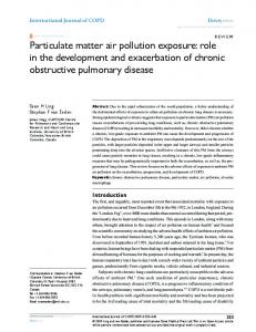
Figure 1: GAM model for ‘At Home’ exposure by temperature, wind speed, hour of the activity and LDEN at the dwelling. The Y-axis shows the exposure correction for BC in ng/m3. Generalized additive models (GAMs) are regression models where smoothing splines are used
3
instead of linear coefficients for the covariates. This approach has been found to be particularly effective for handling the complex non-linearity associated with air pollution research [15-16]. Smooth functions are developed using penalized regression splines, which optimize the fit and try to minimize the number of dimensions in the model. The analysis was constructed using the GAM modeling function in the R environment for statistical computing (R development Core Team, 2009) with the package ‘mgcv’ [17]. 3.2 At Home model For the at-home model the evaluation is made based on the average LDEN for the activity and the average BC exposure during the activity (Figure 1), the summary table is not included for the at-home model. The average exposure is higher for both the high and low temperatures, and shows a minimum for average temperatures. Concentrations decrease with increasing wind speed. The diurnal patterns show an increase for evening activities and a decrease for night activities. Exposure increases with LDEN, but drops for the highest exposures. Since the diurnal patterns used in this evaluation are only sampling 30 dwellings, the statistics of the exposure at home are very sensitive to misclassifications. This is clearly the case for the dwellings where a high exposure was expected. After a manual check, two of the three dwellings could be identified in the vicinity of a major road but screened by buildings from the road. The noise map does not include this screening and results in an overestimation of the local noise exposure. Table 1 – GAM model summary of the in-car model. Parametric coefficients:
(Intercept)
Estimate
Std. Error
t
p-value
5404.0
122.7
44.04