Petre Stoica and Girish Ganesan. Department of Systems and Control,. Information Technology, Uppsala University,. P. O. Box 27, SE-751 03, Uppsala, Sweden ...
TRAINED SPACE-TIME BLOCK DECODING FOR FADING CHANNELS WITH FREQUENCY OFFSETS Petre Stoica and Girish Ganesan Department of Systems and Control, Information Technology, Uppsala University, P. O. Box 27, SE-751 03, Uppsala, Sweden. ABSTRACT Space-time block coding (STBC) is a recent appealing solution to the problem of exploiting transmit diversity in multi-antenna systems for communications over flat fading channels. In a standard STBC scheme the receiver requires Channel State Information (CSI), which can be acquired via training at the expense of a reduced information rate. Alternatively, the requirement of CSI can be avoided altogether by using differential encoding. The existing trained or differential schemes for STBC assume that the channel is timeinvariant during the transmission of at least two data blocks. However, wireless channels may be often time varying owing to frequency offsets induced by either Doppler shifts or carrier frequency mismatches. In this paper we present a simple trained STBC scheme for fading channels with frequency offsets. 1. INTRODUCTION, PRELIMINARIES AND PROBLEM STATEMENT 1.1. Channel Model We consider a wireless communication system with m receive and n transmit antennas. Let t = 1, 2, . . . be the discretetime index expressed in units of the sampling interval. Also, let Akp denote the fading coefficient from the p-th transmit antenna to the k-th receive antenna, and let ωk be the (angular) frequency offset between the k-th receive antenna and the transmit antennas. We assume that ωk is the same (or nearly so) for all transmit antennas. This should be true for the part of ωk induced by a possible carrier frequency mismatch between the transmit and receive oscillators. The previous assumption should also be valid for the Doppler shift part of ωk provided that the multipath components arriving at the receive antennas have similar angles of arrival [7]. Making use of the notation and assumptions introduced above, we can model the output of the receive array as (see [7] for a detailed derivation of the equation below): iω1 t e 0 .. y(t) = (1) A z(t) + e(t) . iωm t 0 e where z(t) is the transmitted (baseband) signal, A = {Akp }, and e(t) denotes a noise term. We assume that {ek (t); for k = 1, . . . m; t = 1, 2, . . .} is a sequence of i.i.d. Gaussian random variables with mean zero and common variance σ 2 . This work was partly supported by the Senior Individual Grant Program of the Swedish Foundation for Strategic Research (SSF).
1.2. Brief Review of STBC Let {sk }P k=1 denote the symbols that we want to transmit in the block b (we omit the dependence of sk on b to simplify notation). In a STBC scheme this is done by transmitting a space-time block (for b = 0, 1, 2, . . .): Zb = [z(N b + 1) . . . z(N b + N )] (n × N )
(2)
that depends on {sk }P k=1 . Following [3, 10] we let Zb depend linearly on {sk }: Zb =
P X [Bk Re(sk ) + i Ck Im(sk )]
(3)
k=1
The matrices {Bk , Ck } in (3) are chosen such that ([2, 3, 4, 5, 10]) ! P X ∗ 2 Z b Zb = |sk | I (4) k=1
where the superscript ∗ denotes the conjugate transpose. The property in (4) of STBC plays a key role in the simplification of the maximum likelihood detector (MLD) for the transmitted symbols (see [3, 10] for details). However the MLD relies on the assumption that the receiver knows A and {ωk } or at least can estimate them accurately. This aspect is discussed next. 1.3. Problem Statement and Discussion of Existing Blind and Differential Schemes Under the assumption that ωk = 0 (k = 1, . . . , m), the channel fading matrix A can be estimated using one or more pilot blocks. A can also be estimated blindly (using only one pilot symbol) or semi-blindly (combining the trained and blind schemes), see the recent paper [8]. The main goal of the present paper is to introduce a simple training-based scheme for the estimation of both A and ωk , which should be the right thing to do in those applications where the frequency offsets cannot be ignored. Owing to the fact that usually transmit diversity is employed when the receiver has rather limited computational capabilities, we aim to keep the complexity of our trained STBC scheme as low as possible. We end this section with a brief discussion of differential encoding as an alternative to acquiring CSI at the receiver via training (in this case the acquired CSI is used in the MLD of a standard STBC scheme. Let us first consider the case in which the frequency offsets are negligible. In a differential scheme (for ωk = 0), the information-bearing block Zb is not transmitted directly; instead, it is differentially encoded in such a way that the MLD based on two consecutive blocks
does not require CSI. Differential STBC schemes achieving this desideratum were recently suggested in [6, 9]. Compared with a trained scheme, a differential scheme does not transmit pilot symbols and hence does not sacrifice information rate. On the other hand, if trading-off information rate for BER performance is what we would like, a trained scheme will do whereas a differential one will not. Additionally, a differential scheme requires unitary symbols (see [6, 9]), while a training-based one has no such restriction. Hence we believe that a differential STBC scheme (such as the ones in [6, 9]) may be useful in fast fading scenarios; otherwise a trained scheme may be preferred . In the perhaps more practically relevant case in which the frequency offsets cannot be ignored, we can think of using double differential encoding in an attempt to avoid the need for CSI at the receiver site. A double differential scheme was recently suggested in [7] for a class of group codes that does not include the STBC considered in this paper. The cited paper trades-off BER performance for computational simplicity. More precisely, the code matrices considered in [7] are diagonal, which limits the achievable BER performance. This resulting performance loss adds to the loss induced by the fact that the detector used is not the MLD (the MLD for double differential encoding is computationally involved even in the single antenna case [11]). Furthermore, our attempts to extend the double differential scheme of [7] to STBC (with non-diagonal code matrices {Zb }) failed to provide a detector with a low complexity. Consequently a trained scheme (such as the one proposed in what follows) may be the way to go whenever the frequency offsets are deemed to be nonnegligible. 2. TRAINED STBC SCHEME Let a∗k denote the k-th row of A, and let yk∗ (b) e∗k (b)
= =
[yk (N b + 1) . . . yk (N b + N )] [ek (N b + 1) . . . ek (N b + N )]
(5)
Using this notation we can write the data equation (1) (for t = N b + 1, . . . , N b + N ) as follows: yk∗ (b) = eiωk N b a∗k Zb Ωk + e∗k (b) (k = 1, . . . , m) where:
eiωk
0 ..
Ωk = 0
.
(6)
(7)
eiN ωk
∗ kyk (b + l) − Ω∗k Zb+l e−iωk N (b+l) ak k2
Z is a square unitary matrix
(10)
To simplify the computations involved, and for lack of a better choice of the pilot blocks, we choose {Zb+l }L l=1 to satisfy (9). Note that if the pilot blocks were chosen as STBC matrices, then satisfying (10) would be possible only for very few values of n. To satisfy (10) for any value of n we do not choose the pilot blocks as STBC matrices but let the pilot block Z to be any unitary n × n matrix. That is: Z ∗ Z = ZZ ∗ = In×n
(11)
(Z can possibly be scaled to satisfy a transmit power constraint). Following the previous discussion, we assume that {Zb+l }L l=1 in (8) satisfy (9) and (10). Consequently, we can write the criterion in (8) as: L X
kZΩk yk (b + l) − e−iωk N l (e−iωk N b ak )k2
(12)
l=1
The minimization of (12) with respect to ak yields: ˆk = a
L X eiωk N b ZΩk eiωk N l yk (b + l) L
(13)
l=1
Inserting (13) in (12) gives the following function which is to be minimized with respect to ωk :
−iN ωk
e I
1 . iN ωk
iN Lωk . I ... e I]
I− . [e
L
e−iN Lωk I 2 ZΩk yk (b + 1)
× ...
ZΩk yk (b + L)
L
2
1 X iN lωk
= const. − e ZΩ y (b + l) (14)
k k
L l=1
2
L
1 X iN lωk
= const. − e yk (b + l) (15)
L l=1
Assume that Zb+1 , . . . , Zb+L are pilot blocks, which hence are known to the receiver (the receiver also knows the time when the transmitter launches the pilot blocks into the channel). We would like to use the pilot blocks and the corresponding received signals, {yk (b + 1), . . . , yk (b + L)}m k=1 , to estimate A and {ωk }. Note that in general we need L ≥ 2 to guarantee the identifiability of both {ak } and {ωk } in (6). Owing to the assumption made on the noise term in (6), the ML estimates of ak and ωk , for given Zb+1 , . . . , Zb+L are obtained by minimizing the following criterion: L X
and
(8)
l=1
As we will see shortly the minimization of (8) becomes simpler if Zb+1 = . . . = Zb+L , Z (9)
Note that if either (9) or (10) were not true then we would have to work with a criterion which would be a more complicated function of ωk than (15) 1 . It follows from (15) that the estimate of ωk is to be obtained by solving the maximization problem:
2 L
X
iωk N l max e yk (b + l) ωk
(16)
l=1
In general estimation of ωk by maximizing (16) is still a bit complicated as it requires a (one-dimensional) nonlinear search. However for L = 2, a closed form expression for ωk can be obtained (see below). For L > 2, to avoid the nonlinear search needed to maximize (16) we can choose L to be even (L = 2K) and approximate the maximizer of (16) as described below. 1 To arrive at (15) from (14) it is not necessary that Z is a STBC. All that is necessary is that Z is unitary.
2.1. The case of L = 2 The criterion (16) with L = 2 has the following simple form: kyk (b + 1) + eiN ωk yk (b + 2)k2 = const. + 2 Re [e−iN ωk yk∗ (b + 2)yk (b + 1)] (17) The value of ωk that maximizes (17) is readily seen to be ω ˆk =
arg [yk∗ (b + 2)yk (b + 1)] N
(18)
The corresponding channel estimate is obtained from (13): iω ˆk N b
ˆk = a
e
2
ˆ k [eiN ωˆ k yk (b + 1) + ei2N ωˆ k yk (b + 2)] (19) ZΩ
Note that in most cases ωk is sufficiently small such that ωk N ≤ 2π. However, if this condition deemed to be invalid in a particular situation, then the simple estimator in (18) should not be used since it will be affected by aliasing. In the latter case, we may let Zb+l depend on l and use the frequency estimate obtained by minimizing the (1D) function of (14) in lieu of that in (15). 2.2. The case of L = 2K (K > 1) In this case we can split the training data set in non-overlapping pairs, {yk (b+1), yk (b+2)}, . . . , {yk (b+2K −1), yk (b+2K)}, estimate ωk and ak from each pair separately using (18) and (19) and average the K so-obtained estimates. While in general the estimates of {ωk and ak } derived in this way are not exact ML estimates, they have lower mean squared error (by a factor of K) than the estimates obtained from just one data pair (this follows easily from the assumptions made on the noise in (6)) and they are easy to compute. To summarize: • In a fast fading scenario we choose L = 2 and estimate {ωk , ak } using (18) and (19). Note that the two training blocks used for acquiring CSI at the receiver do not have to be adjacent to one another. For instance, they can be separated by a STBC data block as shown in Figure 1.
Training
STBC Data
Block n
Block
Training Block
STBC Data Block
N >= n
Figure 1: Transmission scheme for fast fading. The estimation formulas in (18) and (19) can be easily modified to take into account the fact that the transmission rate of the scheme in Figure 1 is P/(N + n), which for N = n = P becomes 1/2. Also note that the scheme relies on the assumption that the channel (i.e, A and {ωk } ) is nearly constant over these blocks (which is basically what a double differential scheme would also require). • For slow fading scenarios we can choose L = 2K with K > 1 and estimate {ωk , ak } by the averaging technique outlined in Section 2.2.
Alternatively, to avoid reducing the transmission rate too much, we can choose L = 2 but unlike the scheme in Figure 1 we insert more than one data block in between the two training blocks. Several other alternative schemes are possible when the fading is not too fast. While we will not dwell into their details, the point we want to make is that a training-based scheme can use the information that the fading is slow to improve the BER performance (possibly at the cost of transmission rate), whereas a (double) differential scheme does not have this flexibility. ˆ k } are used in the MLD, The so-obtained estimates {ˆ ωk , a in lieu of the true unknown values {ωk , ak } to detect the information-bearing symbols transmitted until a new set of pilot blocks is launched into the channel.
3. NUMERICAL EXAMPLES AND CONCLUDING REMARKS In this section we consider the use of the trained STBC scheme discussed in the previous section in a fast fading channel. We consider a system with two transmit antennas and one receive antenna. We assume that the frequency offsets {ωk } are random variables with uniform distribution that lie between 0 and 0.5 radians. The complex channel coefficients {Akp } are assumed to be i.i.d. Gaussian random variables with mean zero and variance 1. This channel model is the same as the one used in [7]. The transmission scheme is as in Figure 1, that is we transmit one training block Z = I2×2 followed by a data block. This is followed by another training block and so on. Thus the effective rate is 1/2. We use the two training blocks adjacent to a particular data block to estimate the channel for that particular data block. In this way we can allow for fast fading channels. The STBC block is an Alamouti code [1] with QPSK constellation. We normalize the STBC such that the corresponding (total) transmitted power is equal to 2, as for the pilot blocks. Since our transmission scheme has rate 1/2 the effective spectral efficiency is 1 b/s/Hz. Simulations were done for 10000 independent channel realizations. In each realization 10 data blocks were transmitted. In Figure 2 we have plotted the Bit Error Rate (BER) for different values of the bit SNR. Plotted also for comparison is the BEP of the double differential scheme in [7] with the same spectral efficiency and total transmit power. From the figure it can be seen that the new scheme outperforms the one in [7] by about 3 dB. Moreover the spacetime block codes we have used are simpler to decode. Finally we remark on the fact that the codes we have considered so far are orthogonal space-time block codes. However the algorithm developed in this paper for channel estimation can be applied to any type of space-time code. In particular the code matrices need not be unitary nor square. The available differential/double differential schemes require the code matrix to be square and unitary.
Acknowledgment We thank the authors of [7] for providing us the MATLAB code for reproducing their simulations.
4. REFERENCES [1] S. M. Alamouti, “A Simple Transmit Diversity Technique for Wireless Communication,” IEEE Jl. on Select Areas in Comm., vol. 16, pp. 1451–1458, October 1998. [2] G. Ganesan and P. Stoica, “Space-time diversity,” in Signal Processing Advances in Wireless & Mobile Communications-Volume 2 (G. Giannakis, Y. Hua, P. Stoica, and L. Tong, eds.), pp. 59–87, New Jersey: Prentice Hall, 2000. [3] G. Ganesan and P. Stoica, “Space-Time Diversity Using Orthogonal and Amicable Orthogonal Designs,” in Proc. of International Conference on Acoustics, Speech and Signal Processing (ICASSP), (Istanbul, Turkey), 2000. [4] G. Ganesan and P. Stoica, “Space-Time Block Codes: A Maximum SNR Approach,” IEEE Trans. on Info. Theory, vol. 47, pp. 1650–1656, May 2001. [5] G. Ganesan and P. Stoica, “Utilizing Space-Time Diversity for Wireless Communications,” Wireless Personal Communications, vol. 18, pp. 149–163, August 2001.
0
10
Detection scheme using OSTBC Double differential scheme using diagonal STBC
[6] G. Ganesan and P. Stoica, “Differential Detection Based on Space-Time Block Codes,” 2002. To appear in Wireless Personal Communications.
[8] P. Stoica and G. Ganesan, “Space-Time Block Codes: Trained, Blind and Semi-Blind Detection,” 2002. To appear in Digital Signal Processing - A review Journal. [9] V. Tarokh and H. Jafarkhani, “A Differential Detection Scheme for Transmit Diversity,” IEEE Journal on Selected Areas in Communication, vol. 18, pp. 1169–1174, July 2000. [10] V. Tarokh, H. Jafarkhani, and A. R. Calderbank, “Space-Time Block Codes from Orthogonal Designs,” IEEE Trans. on Info. Theory, vol. 45, pp. 1456–1467, July 1999. [11] D. K. van Alphen and W. C. Lindsey, “Higher-Order Differential Phase Shift Keyed Modulation,” IEEE Transactions on Communications, vol. 42, pp. 440–448, February/March/April 1994.
−1
10 Bit Error Rate
[7] Z. Liu, G. B. Giannakis, and B. L. Hughes, “Double Differential Space-Time Block Coding For Time-Selective Fading Channels,” IEEE Transactions on Communications, vol. 49, pp. 1529–1539, September 2001.
−2
10
−3
10
−4
10
3 4 5 6 7 8 9 10 11 12 13 14 15 16 17 18 19 20 21 22 23
SNR
Figure 2: Bit Error Rates for the proposed detection scheme and the scheme in [7]