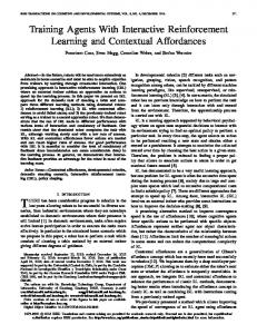
Training and Delayed Reinforcements in Q-Learning Agents - CiteSeerX

Training and Delayed Reinforcements in Q-Learning Agents

TR/IRIDIA/1994-14 Université Libre de Bruxelles Belgium

Pierguido V. C. Caironi Progetto di Intelligenza Artificiale e Robotica, Dipartimento di Elettronica e Informazione, Politecnico di Milano, Piazza Leonardo da Vinci 32, 20133 Milano, Italy [email protected] Marco Dorigo IRIDIA, Université Libre de Bruxelles, Avenue Franklin Roosevelt 50, CP 194/6, 1050 Bruxelles, Belgium [email protected], http://iridia.ulb.ac.be/dorigo/dorigo.html

Abstract Q-learning can greatly improve its convergence speed if helped by immediate reinforcements provided by a trainer able to judge the usefulness of actions as stage setting with respect to the goal of the agent. This paper experimentally investigates this hypothesis studying the integration of immediate reinforcements (also called training reinforcements) with standard delayed reinforcements (namely, reinforcements assigned only when the agent-environment relationship reaches a peculiar state, such as when the agent reaches a target). The paper proposes two new algorithms (TL and MTL) able to exploit even locally wrong and misleading training reinforcements. The proposed algorithms are tested against Q-learning and other algorithms (AB-LEC and BB-LEC) described in the literature1 which also make use of training reinforcements. Experiments are run in a grid world where a Q-agent, a simple simulated robot, must learn to reach a target.

Accepted for publication in International Journal of Intelligent Systems, 1997. In press.

Caironi and Dorigo - Training and Delayed Reinforcements in Q-Learning Agents

1/33

I. INTRODUCTION Reinforcement learning, which is learning driven by scalar values given to the learner to reinforce its behavior, is a promising area of machine learning. So far, many algorithms have been proposed in this domain, namely, Temporal Differences2 and derived algorithms: Adaptive Heuristic Critic3,4, Learning Classifier Systems5 and Q-learning6. Unfortunately, if rewards are given to the learner only when it reaches its intended goal, even the best reinforcement learning algorithms converge too slowly to the optimal solution to be applicable in most real world problems1,7. This is because the agent, starting from null-knowledge, wastes a huge amount of time exploring uninteresting areas of the environment. Some form of pre-coded knowledge such as a good exploration strategy or an initialization of action-values may be used to ease this problem. Regarding the exploration strategy, this has been already discussed in other works 8 and the results of these works may be easily applied to what is presented in this paper. For what concerns action-values initialization, we believe that this approach is extremely useful in practical applications, but it is too close to an explicit programming of the agent to be of real interest for machine learning researchers. Besides, a correct initialization of action-values may be not so easy to achieve. Thus, we focused on a different approach: the use of immediate reinforcements provided by a trainer. The goal of the trainer is to exploit his knowledge to focus the exploration of the learning agent. In this paper we call delayed reinforcements the reinforcements given to the agent when a manifest and peculiar state in the agent-environment system is reached (e.g., when the agent reaches the goal) and training reinforcements the immediate reinforcements given by the trainer. The distinction between training and delayed reinforcement does not reside in any quantitative difference (such as in the frequency they are given to the agent or in their absolute value) but in their origin. For example, getting into the goal state or smashing into an obstacle are typical situations that can trigger a delayed reinforcement since they usually represent a macroscopic event in the environment. On the contrary, an action that lowers the distance of the agent from the goal but that does not take directly the agent into the goal can only be rewarded by a trainer since its interpretation requires a non-trivial knowledge (i.e., the trainer can reward this action only if he knows that a reduction of the distance between the agent and the goal is a stage-setting event to get into the goal state). Actually, training reinforcement may be seen as a way to transfer knowledge from the trainer to the agent 9. Training reinforcements are obviously more useful when the environment does not lend itself to produce many delayed reinforcements. Indeed, this is a frequent case according to our experience. The purpose of this article is to study how to integrate training reinforcements with delayed reinforcements in the context of Q-learning. Our experience has shown this is not a trivial Caironi and Dorigo - Training and Delayed Reinforcements in Q-Learning Agents

2/33

problem. A first difficulty was identified by Whitehead1 and refers to the so-called extinction effect, which appears after the training reinforcement is, for any reason, suspended. This suspension can confuse the agent about the value of its actions. A second important issue is the correctness of training reinforcements. The design or availability of a perfect trainer, that is, of a trainer who always provides correct reinforcements, may be both difficult and expensive. For the reason of practical feasibility, it is therefore necessary to accept trainers liable to be inaccurate10,11,12 or even, at times, wrong in wide areas of the search space, and study learning algorithms which are robust to trainer's inaccuracies. In this article, together with a perfect training reinforcement, we explore two kinds of incorrect training reinforcements: locally wrong and misleading. Locally wrong training reinforcements model an inaccurate trainer whose reinforcements are systematically mistaken for some state-action pairs. A misleading training reinforcement is a reinforcement that does not lead the agent to the goal and cause the agent to get trapped in some other area of the search space (e.g., inside the concavity of an obstacle). To cope with these incorrect reinforcements, we present two new algorithms. The first algorithm is called Trusting Learner (TL) and it is devised to exploit locally wrong training reinforcements without getting trapped in the possible small local minima that such reinforcements can introduce. The second algorithm is called Modified Trusting Learner (MTL) and it is an extension of TL designed to intentionally ignore training reinforcements in areas of the search space where they are misleading. Besides, MTL shows adaptive capabilities which allow the efficient solution of the blocking problem13. Preliminary to the exposition of our algorithms, we discuss the action choice methods used in our experiments and point out a peculiarity of the method based on the Boltzmann distribution. All the algorithms we propose are tested in the context of a simple simulated robotic environment against Q-learning and two other algorithms, AB-LEC and BB-LEC 1, which are tightly related to the ideas we discuss in the article. The testing environment is a typical grid world where a robot, called Q-agent, tries to reach a definite position known as goal. To learn which actions to perform in order to reach the goal, the agent receives a delayed reinforcement whenever it reaches the goal, a positive training reinforcement when it performs an action that lowers its distance from the goal and a negative training reinforcement when it performs an action that increments it.


3/33

II.

Q-LEARNING AND ACTION CHOICE

Q-learning 6 is a reinforcement learning algorithm inspired by stochastic dynamic programming. Let S be the set of states as seen by the Q-agent through its sensory system, and A(s) be the set of actions executable in a state s ∈S. Given the following definition for the discounted reinforcement V γ (s,a) of a state-action pair (s,a): ∞ t  V (s,a) = E ∑ γ ⋅ rt (st ,at ) s0 = s, a0 = a  ,  t =0  γ

(1)

where γ is the discount factor and rt(st,at) is the reinforcement given at time t after executing action at in state st, Q-learning assigns to each state-action pair (s,a) a value (called Q-value) which is an approximation of the discounted reinforcement obtained executing action a in sensory state s and then choosing in each following state s' the action b that maximizes Q(s',b). The formulae used by Q-learning to update the Q-values are: V(st +1 ) ← max Q(st +1 ,a)

(2)

Q(st ,at ) ← (1 − α) ⋅ Q(st ,at ) + α ⋅ (rt + γ ⋅ V(st +1 )) .

(3)

a∈A(st +1 )

where α is a constant coefficient belonging to the interval (0,1]. Formulae (2) and (3) can be used either after executing each action, which is what we call the standard Q-learning, or, after reaching the goal and having received a delayed reinforcement, starting from the most recently experienced state-action pair and going backward to the stateaction pair experienced immediately after the second last delayed reinforcement. This latter kind of update order, as far as we know, was first proposed by Lin 14, and it is usually referred to as backward Q-learning. A.

Action Choice

Obviously, if a Q-agent desires to obtain the highest expected discounted reinforcement, it has to choose, in each state, the action with the highest Q-value. However, especially at the beginning of learning when the agent has experienced just a few state-action pairs, the Q-values may be widely inaccurate in representing the correct discounted reinforcements. Always choosing the highest Q-value action would lead the Q-agent to follow always the same path not exploring possibly better solutions. From time to time it is therefore advisable to choose exploration actions, that is, actions not optimal according to the current Q-values. Many methods have been suggested to choose these actions such as counter, recency and error based exploration 8 or exploration bonus in Dyna-Q13.


4/33

Because of their simplicity and their practical suitability to the kind of application proposed in this article, we consider only the two methods most often used in literature, the Boltzmann distribution and the pseudo-stochastic choice (the latter is sometimes called the semi-uniform distribution), and we compare them against our method called the pseudo-exhaustive choice. •

Boltzmann distribution. An action a belonging to the set of possible actions A(s) has the following probability of being chosen in state s :

p(a ) =

Q(s,a ) e T

∑

Q(s,a) e T

(4)

a∈A(s)

where T is a constant called temperature that controls the degree of randomness of the choice. •

Pseudo-stochastic method. In a given state s the action with the highest Q-value has an initial probability Ps of being chosen. If the action with the highest Q-value is not chosen, then the Q-agent chooses an action randomly (with uniform probability distribution) among all the possible actions of the current state (including the action with the highest Q-value).

•

Pseudo-exhaustive method. In a given state s the action with the highest Q-value has a probability Pe of being chosen. If the action with the highest Q-value is not chosen, then the Q-agent executes the action least recently chosen in the current state.

The experiments reported in Section V (Subsection A) show that the pseudo-exhaustive method is able to lead the agent to better performance. Because of this good performance and its low computational overhead, we used the pseudo-exhaustive method for all the experiments presented in the paper. We noticed that Boltzmann distribution method is clearly the worst of the three. Using this method the Q-agent chooses too many exploration actions in states far from the goal and does not explore enough states close to the goal. This result is due to the non-linearity of exponentials present in equation (4). Taking two states with the same ratio between Q-values but with different averages, the action with the highest Q-value will have a greater probability of being chosen in the state with higher average (see Appendix A). Considering that average Qvalues tend to be higher in states near to the goal and lower in states far from the goal, using the Boltzmann distribution method the Q-agent usually chooses too few exploration actions in states close to the goal and too many exploration actions in states far from the goal.


5/33

III. THE ALGORITHMS Before analyzing the details of each algorithm let us consider Figure 1 which represents the structure of the typical learning system used by our learning agents, and its relationship with the simulated environment and the trainer. The reinforcement learning algorithm receives the delayed and training reinforcements as well as the sensory data describing the current physical state of the environment and decides which action the agent has to perform. The delayed reinforcement computing system is generally a simple sensory system able to recognize a particular goal state in the environment and to produce a signal, the delayed reinforcement, after this state has been reached. The trainer, if active, examines the environment and assigns to the agent a training reinforcement computed on the basis of the state (or change of state) produced in the environment by the last action of the agent. In this paper, for simplicity, we have always considered an artificial trainer (e.g., a device installed in the robot's body) but it should be possible to use a human trainer.

Agent Delayed reinforcement computing system

Sensory data

Sensors of the agent

Sensory stimuli

Environment

Delayed reinforcement

Sensory data

Reinforcement learning algorithm

Training reinforcement

Proposed actions

Effectors

Trainer

Actions

Sensory stimuli

Figure 1. Agent's structure and its relationship with the environment and the trainer

A.

The AB-LEC Algorithm

This algorithm, proposed by Whitehead1, represents the most obvious approach to the problem of integrating training and delayed reinforcements. The training reinforcement is, when present, simply added to the delayed reinforcement to make a single reinforcement which is then used in formula (3) to update the Q-value of the last experienced state-action pair.


6/33

Although easy to implement, this algorithm performs quite poorly if, for any reason, after a certain number of cycles the training reinforcement ceases to be given. On this occasion, the Qagent seems to forget everything it has learnt up to that point and starts to behave in a chaotic way showing what Whitehead has called extinction effect. The relevance of the extinction effect is proportional to the increment the training reinforcement produces in the Q-values as compared to the value they would have if computed using only delayed reinforcement. During the training phase the sum of the training and delayed reinforcements causes the Qvalues to reach a high value. As soon as training reinforcements are no longer assigned, new updatings, even if based on positive delayed reinforcements, reduce the Q-values of the stateaction pairs to which they are applied. This phenomenon lowers all the Q-values of the stateaction pairs belonging to the optimal policy to a level inferior or equal to the Q-values of suboptimal state-action pairs that have not yet been updated. This leveling destroys the effect of the training reinforcement received up to that point making the trainer useless. Considering the possibility of an interruption in the training reinforcement is by no means trivial: if the trainer is not an electronic device, but a human expert, his monitoring of the learning agent will eventually end or have pauses. Besides, even if the trainer is an electronic device, there could be situations in which the trainer, especially if expensive and equipped with sophisticated hardware or sensors, could be better exploited if used to train another robot instead of just one (for a general discussion of the role of the trainer in reinforcement learning see the works of Dorigo and Colombetti9,11,12). Experiments (reported in Section V, Subsection B) show that lowering the ratio between the values of the training and the delayed reinforcements, can effectively reduce the relevance of the extinction effect since in this way the importance of the training reinforcement in the Q-values is reduced. Nonetheless, this problem, together with the extreme sensibility of this algorithm to locally wrong training reinforcement (see again Section V, Subsection B) makes AB-LEC not advisable for a practical robotic application. B.

The BB-LEC Algorithm

This algorithm has been proposed by Whitehead1 to overcome the extinction effect. In BBLEC the training and delayed reinforcements are not added together. The delayed reinforcement is used as in standard Q-learning (equations (2) and (3)) to update the Q-values table, whereas the training reinforcements are used to produce the biasing values B(s,a). These biasing values are scalar values memorized in a separate table of the same dimensions of the Qlearning one. They are updated according to the following formula: B(st ,at ) ← (1 − ψ) ⋅ B(st ,at ) + ψ ⋅ rt′′


(5)

7/33

where rt′′ is the training reinforcement received after executing action at in state st at time t, and ψ is a constant coefficient belonging to the interval (0,1]. In BB-LEC, action choice is not based on Q-values alone, as in Q-learning and AB-LEC, but on the sum of Q-values and biasing values. In the experiments (see Section V, Subsections B and C) we test also a backward version of BB-LEC, not considered by Whitehead. While the standard version of BB-LEC shows some problems with locally wrong training reinforcements, the backward version is able to withstand training reinforcements of poor quality achieving better results than standard Q-learning. Unfortunately, these good capabilities are, like in AB-LEC, sensitive to the ratio between the average values of training and delayed reinforcements. This is because the action choice is a function of the sum of the Q-values and the biasing values. If the average value of the training reinforcements is too high and the training reinforcements are wrong, incorrect biasing values may dominate the Q-values (especially in states far from the goal where Q-values are lower) forcing the Q-agent to choose wrong actions. C.

The TL Algorithm

We designed the TL algorithm (see Figure 2) to avoid the need to tune the ratio between training and delayed reinforcements, which in real robots is a time consuming task, and to cope with locally wrong training reinforcement, that is reinforcement affected by a systematic error with a null expected value (see Section IV, Subsection A). To obtain these results, first of all, we partitioned the entire learning session in trials. With trial we mean the period of time spanning from the assignment of a delayed reinforcement to the next assignment (this partition of the learning session is consistent with what happens in backward Q-learning where, at the end of each trial, the update of the Q-values takes place). Exploiting this temporal partition, the TL algorithm introduces a distinction between known states, which are states experienced during trials preceding the current one, and new states, which are states encountered for the first time in the current trial (i.e., states encountered for the first time after the last assignment of the delayed reinforcement). While the Q-values of known states are updated only at the end of the trial using backward Q-learning based on delayed reinforcement alone, the Q-values of new states are continuously updated using training reinforcements as new Q-values. Since a certain state can be either known or new but not both, Q-values computed with different kinds of reinforcements never mix in the same state, and, therefore, action choice does not depend (as in AB-LEC or BB-LEC) on the ratio of training and delayed reinforcements. When the agent reaches the goal, it examines each state-action pair experienced during the last trial going backward from the last state encountered to the first one.


8/33

If the last state of the trial (the state from which the agent entered the goal state) is a known state, its Q-values are updated using Q-learning equation. If it is a new state, its Q-values are reset before doing normal Q-learning update. That is, delayed reinforcement completely overrides training reinforcement in this state where the delayed reinforcement has been directly received. The procedure applied to the other state-action pairs of the trial is a slightly different. Each state s is examined separately. If it is a known state, its Q-values are updated according to standard Q-learning rules. If it is a new state, the action actually executed is discarded and its Q-values are scanned to find the action amax with the highest Q-value. All Q-values are reset to zero and then the Q-value of action amax is updated according to Q-learning equation as if it were the action actually executed. Then state s is inserted in the set of known state and the procedure continues with another state. Reset Q-values: Q(s,a) ← 0, ∀s ∈ S , ∀a ∈ A( s). Initialize the set I of known states: I ← ∅. Empty the LIFO queue L of states experienced in the current trial. REPEAT Get current state st and choose and execute action at. Get the new current state st+1, the delayed reinforcement rt′ ( rt′ =0 if not assigned) and the training reinforcement rt′′ ( rt′′ =0 if not assigned). IF ( rt′ =0) THEN /* the delayed reinforcement has not been assigned */ Push (st,at) in L. IF ( st ∉ I ) THEN /* the state st is new */ Q(st,at) ← rt′′ ENDIF ELSE /* rt′ ≠0: the delayed reinforcement has been assigned */ IF ( st ∉ I ) THEN /* the last state of the trial was a new state */ Q(st,a) ← 0, ∀a ∈ A(st) I ← I ∪ {st} ENDIF Q( st ,at ) ← ( 1 − α) ⋅ Q( st ,at ) + α ⋅ rt′ /* Execute backward Q-learning for each state-action pair in L */ sk + 1 ← st WHILE (L is not empty) Extract a state-action pair (sk,ak) from queue L. V( sk + 1 ) ← max Q( sk + 1 ,a) a ∈A( sk + 1 )

IF ( sk ∉ I ) THEN /* the state sk was new */ ak ← b, with b such that Q(sk,b) ≥ Q(sk,a), ∀a ∈ A(sk) Q(sk,a) ← 0, ∀a ∈ A(sk) I ← I ∪ {sk} ENDIF Q( sk ,ak ) ← ( 1 − α) ⋅ Q( sk ,ak ) + α ⋅ γ ⋅ V( sk + 1 ) sk + 1 ← sk ENDWHILE ENDIF UNTIL (the required number of cycles has been made) Figure 2. The TL algorithm (the symbol

← means “assignment to a variable”)


9/33

Using this update policy the action amax that the trainer considers the best (since it has the highest training Q-value) gets an initial advantage over all the others (since it is the only one to be updated with a non-null Q-value). The updates executed in the following trials, being based on delayed reinforcement (as from now on the former new states belong to the set of known states), may reconfirm or eliminate this advantage. As we have said, training reinforcements affect only new states. This fact reduces the effect of possibly wrong training reinforcements and confines the relevance of the trainer to the first phase of exploration. As the Q-agent gets confident with the environment and increments, trial after trial, the number of known states, the role of training reinforcements becomes gradually less important. This permits a good trade-off between trust in the trainer and trust in agent’s experience represented by Q-values of known states. D.

The MTL Algorithm

We propose the MTL algorithm (see Figure 3) to overcome the problems caused by misleading reinforcements, that is reinforcements so systematically mistaken in wide areas of the state space as to divert the Q-agent from the goal (see the grid with obstacle experiment in Section IV for an example of this kind of reinforcement). MTL treats Q-values almost in the same way as the TL algorithm does (and inherits the same robustness to locally wrong training reinforcements and indifference to the ratio between training and delayed reinforcements), but can “distrust” Q-values on the ground of the number of times that the Q-agent has entered the state which they belong to. Let us define the trust function f(.) (a decreasing sigmoid function):

f (n(s)) =

1+ e 1+ e

 1−no   ⋅pf  no 

 n(s)−no   ⋅pf  no 

,

(6)

with pf and no two empirically determined constant coefficients and n(s) equal to the number of times the Q-agent has entered state s during the current trial. Figure 4 shows a plot of equation (6) for no=50 and pf =10.


10/33

Reset Q-values: Q(s,a) ← 0, ∀s ∈ S , ∀a ∈ A( s). Initialize the set I of known states: I ← ∅. Empty the LIFO queue L of states experienced in the current trial. Reset the counters n(s) ← 0, ∀s ∈ S . REPEAT Get current state st and let n(st) ← n(st) + 1. Choose action at considering the trust function f( n( st )). Execute action a t and get the new current state s t+1 , the delayed reinforcement

rt′

( rt′ =0

if

not

assigned)

and

the

training

reinforcement rt′′ ( rt′′ =0 if not assigned). IF ( rt′ =0)

THEN /* the delayed reinforcement has not been assigned */

Push (st,at) in L. IF ( st ∉ I ) THEN /* the state st is new */ Q(st,at) ← rt′′ ENDIF ELSE /* rt′ ≠0: the delayed reinforcement has been assigned */ IF ( st ∉ I ) THEN /* the last state of the trial was a new state */ Q(st,a) ← 0, ∀a ∈ A( st ) I ← I ∪ {st} ENDIF Q( st ,at ) ← ( 1 − α) ⋅ f( n( st )) ⋅ Q( st ,at ) + α ⋅ rt′ /* Execute backward Q-learning for each state-action pair in L */ sk + 1 ← st WHILE (L is not empty) Extract a state-action pair (sk,ak) from queue L. V( sk + 1 ) ← max Q( sk + 1 ,a) a ∈A( sk + 1 )

IF ( sk ∉ I ) THEN /* the state sk was new */ IF ( n( sk ) < no ) THEN /* sk is a trustable state */ ak ← b, with b such that Q(sk,b)≥Q(sk,a), ∀a∈A(sk) ENDIF Q(sk,a) ← 0, ∀a ∈ A(sk) I ← I ∪ {sk} ENDIF Q( sk ,ak ) ← ( 1 − α) ⋅ f( n( sk )) ⋅ Q( sk ,ak ) + α ⋅ γ ⋅ V( sk + 1 ) sk + 1 ← sk ENDWHILE n(s) ← 0, ∀s ∈ S ENDIF UNTIL (the required number of cycles has been made) Figure 3. The MTL algorithm (the symbol

← means “assignment to a variable”)

1 0.9 0.8

n0=50 Pf=10

f(n(s))

0.7 0.6 0.5 0.4 0.3 0.2 0.1 0 0

10

20

30

40

50

60

70

80

90

100

n(s)

Figure 4. Plot of equation (6) for no=50 and pf=10


11/33

Since Q-values of states frequently entered during the same trial probably belong to a suboptimal cyclic policy, MTL tries to reduce their impact on the policy of the Q-agent. This is achieved by choosing actions with a higher degree of randomness in states more frequently entered. In the pseudo-exhaustive and pseudo-stochastic methods this higher randomness is obtained by multiplying the probability of choosing the action with maximum Q-value by the trust function of the current state; in the Boltzmann method by multiplying the temperature T by 1 f (n(s)). Moreover, Q-values of known states are multiplied by the trust function before being updated at the end of the trial and Q-values of new states affect Q-values computation at the end of the trial only if they are trustable. We mean by this that in new states Q-values are treated as described in the previous section only if the agent has entered that state during the last trial less than n 0 times. If this condition does not hold, training Q-values are totally discarded and traditional Q-learning update based on delayed reinforcement is applied. We have designed this algorithm to distrust Q-values computed with misleading training reinforcements in new states, but it is able to deal even with incorrect Q-values in known states. For example, let us consider the blocking problem 13, in which, after the Q-agent has developed a certain policy to reach the goal, the appearance of a new obstacle on the usual trajectory makes the policy developed up to that point inadequate to the new situation. In this case, after uselessly bumping against the obstacle a certain number of times, the trust function of states belonging to the old trajectory starts to decrease. Since a decreasing trust function means an increase in the number of exploration actions, the robot increases its exploration near the obstacle till it finds a way around it.

IV. THE EXPERIMENTAL SETUP The experimental setup comprises a set of simulated environments chosen to test each relevant aspect of the algorithms discussed in the article. All the environments are based on the typical grid world often used in Q-learning literature 1,13,15. The map of these environments (see Figure 5) is based on a rectangular grid of cells. Each cell represents a possible position. The Q-agent starts the simulation in a given position S and then moves, each time tick, into one of the four cells next to the one it is currently in. There are cells occupied by obstacles (gray cells in Figures 5 and 6) that cannot be entered by the Q-agent. If the Q-agent tries to move into one of these cells, the action will result in no actual movement. The relation between each state-action pair and the next state is deterministic (that is, a particular action in a particular state causes the system to reach always the same next state). The purpose of the Q-agent is to reach the goal cell G. Each time the Q-agent reaches the goal it is assigned the delayed reinforcement r′ =1 and it is transported back to the starting point


12/33

S to experience a new trial. The training reinforcement is computed after each action according to the change in the Manhattan distance between the Q-agent and the goal (see next subsection). The sensory input of the Q-agent is represented by the two coordinates of its position. Since all the other components of the environment have a fixed position, the Q-agent enjoys complete state information. We considered two kinds of maps: the first is a free grid, i.e., a grid of empty cells surrounded by walls (Figure 5); the second (Figure 6) is the grid with obstacle map, a grid with a concave obstacle between the starting point S and the goal G.

S

G

Figure 5. The free grid map

S

G

Figure 6. The grid with obstacle map

Three experiments have been executed in the maps described. • Free grid experiment. In this experiment the Q-agent moves in the map of Figure 5. The experiment is divided in two consecutive phases each one lasting fifty trials. During the first phase, which is called training phase, the Q-agent receives both training and delayed reinforcements; in the second phase, called delayed phase, it receives just delayed reinforcements. The purpose of the first phase is to test the capabilities of the various algorithms to exploit the training reinforcements (whether locally wrong or not). The second phase is intended to show possible extinction effects. In this environment we have tested Qlearning, AB-LEC, BB-LEC and TL.


13/33

• Grid with obstacle experiment. This experiment is identical to the previous one except for the map used which is the one represented in Figure 6. The goal of this experiment is to test the MTL algorithm in a situation where the training reinforcement is misleading, that is, when the reinforcement directs the agent towards the concavity of the obstacle. • Blocking problem experiment. This experiment is an extension of the free grid experiment. It is composed of three phases of 50 trials each: the first two are identical to the ones described in the free grid experiment and are executed in the map of Figure 5; the third one (second delayed phase) is executed in the map of Figure 6 using only delayed reinforcements and making the agent start its trial from the same starting cell S it has in the free grid map (i.e., third column on the left, center row - see Figure 5). The purpose of this last phase is to show the capability of the MTL algorithm to solve the blocking problem, that is to adapt the policy learned in the free grid map to the new grid with the obstacle. After each learning phase (training, delayed or second delayed), during which the Q-agent chooses actions according to one of the algorithms described in Section III, there is a test trial. During this trial the learning algorithm is switched off and the Q-agent is forced to choose, in each state, the action with the highest Q-value. The purpose of this test trial is to measure the length of the optimal trajectory found by the Q-agent up to that moment. To give a statistically significant measure of the performance of each learning algorithm, we have run 100 experiments for each combination of algorithm, environment and parameter values (we call one of these sets of 100 experiments a population) and based our comparison on average performance computed on these populations. In Section V the convergence process during the learning, delayed and second delayed phases is represented by graphs that show the average length of each trial for the various populations. The results of the test trials are represented by tables showing averages and standard deviations of trial lengths of Q-agents which succeeded in reaching the goal. If relevant, the percentage of Q-agents able to reach the goal during the testing trials is shown. To prove the statistical significance of the conclusions we drew from the results of the test trials we used Kruskal-Wallis ANOVA and Mann-Whitney U-Test16. A.

Computation of Training Reinforcements

In all the experiments, the training reinforcement rt′′ is computed according to the formula rt′′ = −R ⋅ sign(dt − dt −1 ) , (7) where R is a definite constant, sign is the sign function  1 if z > 0,  sign(z) =  0 if z = 0, −1 if z < 0,  Caironi and Dorigo - Training and Delayed Reinforcements in Q-Learning Agents

(8)

14/33

and dt is the Manhattan distance of the agent from the goal at time t computed according to the following formula dt = xt − x + yt − y ,

(9)

where (xt,yt) and ( x , y ) are the co-ordinates of the agent at time t and of the goal respectively. Thus, if the last action has reduced the Manhattan distance dt , the Q-agent gets a r ′′ = + R reinforcement, otherwise it gets a −R punishment. If there are no obstacles in the map, as in Figure 5, equation (9) generates perfect training reinforcement. If there are obstacles in the map, as in Figure 6, equation (9) generates misleading reinforcements, since it does not consider the presence of obstacles between the agent and the goal. In fact, in the area on the left of the obstacle, the agent receives positive reinforcement even when it approaches the obstacle and gets trapped inside it. In our experiments we also considered a locally wrong training reinforcement. This reinforcement is affected by a systematic error, that is, it is always wrong in the same way for the same state-action pair. In fact, this is the worst kind of local error in training reinforcement, since its influence on Q-values cannot be eliminated by averaging on different reinforcement samples. Locally wrong reinforcement has been obtained using, instead of equation (9), the formula

(

)

dt = xt − ( x + nx ) + yt − y + ny ,

(10)

where nx and ny are the error components. The values nx and ny are a function of the position (x,y) from where the training system computes the distance dt (i.e., the position of the agent). Functions n x(x,y) and n y(x,y) are represented by two constant matrixes, generated at the beginning of the simulation, that assign to each possible (x,y) position of the agent two error components (nx,ny). The two matrixes are created using a random number generator producing integer numbers in the set [−2,+2] with the probability distribution reported in Table 1. Table 1. Probability distribution of error components (nx,ny) in locally wrong training reinforcement. Probability nx or ny value

0.125 −2

0.25 −1

0.25 0


0.25 +1

0.125 +2

15/33

V.

EXPERIMENTAL RESULTS A.

Action Choice

The purpose of the experiments reported in this section is to compare the three action choice methods (Boltzmann, pseudo-stochastic and pseudo-exhaustive) described in Section II. The experiments are executed in the free grid map (Figure 5). To avoid any complication due to training, we tested the action choice methods using standard backward Q-learning without any kind of training reinforcement. Since there is no training, we have considered a single learning phase of 100 trials. In order to have a meaningful way of comparing Q-agents using different action choice methods, during the learning phase we forced the average length of trials to be approximately of a same length. This way it was possible to compare the ability of each action choice method to obtain good performance using the same average number of exploration actions. Since there is no way to force the Q-agent to execute trials of exactly a desired lengths, we empirically found values for the parameters T, Ps and Pe which produced trials of average length close to the desired one. Table 2 reports the results of the experiments. We divided these experiments in 3 sets, each one with a different “desired average learning trial length” (45, 75 and 110 cycles). In the column labeled “actual average learning trial length” is reported the actual average length of the trials during the learning phase. These actual average lengths do not consider the first trial since, all Q-values being zero, in the first trial all actions are chosen completely randomly and independently of the action choice method. The “average test trial length” shows the average lengths of trials during the testing phase. As previously said, during this phase there are no exploration actions, that is, chosen actions are the ones with highest Q-values. The average test trial lengths show that Boltzmann exploration generates longer (thus, worse) average lengths during testing trials than the other two action choice methods; also, the pseudo-exhaustive method consistently outperforms both the Boltzmann and the pseudostochastic methods. Kruskal-Wallis ANOVA applied among the populations of each group of equal average learning trial length always gave a p-level less than 10− 3 . Mann-Whitney U-tests showed that all the performance differences between pseudo-exhaustive action choice method and Boltzmann or pseudo-stochastic action choice methods are significant (p-level < 0.03), except for the difference between pseudo-exhaustive and pseudo-stochastic methods in the 45 average length group. This is probably because in this length group the exploration actions during


16/33

learning are too few, and the performance differences among exploration algorithms tend to vanish. Given the results of this section we decided to use pseudo-exhaustive action choice method for all the experiments reported in the following sections. Table 2. Comparison among action choice methods (the minimal optimal trial length is 21) Action choice method

Parameters values

Boltzmann

T = 8.3·10−5

Pseudo-stochastic

Ps= 0.88

Pseudo-exhaustive

Pe= 0.9

45 −4

Boltzmann

T = 7,1·10

Pseudo-stochastic

Ps= 0.5

Pseudo-exhaustive

Pe= 0.6

Boltzmann

T = 2.5·10−3

Pseudo-stochastic

Ps= 0.33

Pseudo-exhaustive

Pe= 0.45

B.

Desired average Actual average learning trial learning trial length length

75

110

Average test trial length

Standard deviation of test trial length

48.04

35.56

5.16

43.30

31.58

5.51

43.02

30.88

4.29

75.28

32.68

4.14

75.30

24.46

2.76

71.93

23.70

2.73

116.34

30.64

3.50

114.57

21.80

1.14

105.94

21.28

0.75

AB-LEC and BB-LEC in the Free Grid Experiment

In this section we show the results of experiments run using the AB-LEC and BB-LEC algorithms proposed by Whitehead1. This allows us to discuss their problems and to put our research in context. The average lengths of the learning trials for three AB-LEC populations in the free grid experiment with locally wrong training reinforcement are reported in Figure 7. In order to change the ratio between training and delayed reinforcements we have kept the delayed reinforcement value to 1 and set the training reinforcement absolute value R to 1, 10− 2 and 10− 4 . The population with R = 1 shows an evident extinction effect (the peak in the dotted line) after the beginning of the delayed phase at trial 51. In the other two populations the extinction effect is less evident, however the convergence during the training phase results nonetheless quite “bumpy” due to the high sensitivity of AB-LEC to locally wrong training reinforcements. In Table 3 we report the results of testing phase trials executed after training and delayed phases respectively. In these tables there is also the percentage of the Q-agents which were able to reach the goal during the test trial.


17/33

700 R=1

Average trial length

600

R=0.01

500

R=0.0001

400 300 200 100 0 0

10

20

30

40

50

60

70

80

90

100

Number of trials

Figure 7. AB-LEC in the free grid experiment with locally wrong training reinforcement

These results, and especially the low percentage of Q-agents which reach the goal, show clearly the difficulty that AB-LEC has in dealing with locally wrong training reinforcements and extinction effect. Using perfect training reinforcements and choosing the correct value for the parameter R, the performance of this algorithm can drastically improve, however, in the situation tested in the experiments discussed in this section, the average length of the learning trials of AB-LEC was greater (and therefore worse) than that of backward Q-learning during all the training phase. Table 3. AB-LEC in the free grid experiment with locally wrong training reinforcement: results of the test trials (the minimal optimal trial length is 21) Test trial after the training phase

Test trial after the delayed phase

Value of R Q-agents which Average length Std deviation Q-agents which Average length Std deviation reach the goal of trial of trial reach the goal of trial of trial R=1

28%

27.00

3.17

0%

-

-

R=10−2

83%

24.69

2.20

96%

22.13

1.32

R=10−4

98%

24.86

2.67

100%

23.26

1.92

We have repeated the experiments just described for AB-LEC with standard and backward BB-LEC. The extinction effect, even if reduced, is still present (see Figures 8 and 9, the peaks in the dotted lines after the 51st trial). As you may notice comparing Figures 8 and 9, backward BB-LEC has a convergence speed clearly superior to standard BB-LEC, but Tables 4 and 5 show that with both standard and backward BB-LEC many Q-agents are unable to reach the goal in the test trial after the training phase. This problem is due to locally wrong training reinforcement and its relevance is clearly a function of the parameter R.


18/33

Table 4. Standard BB-LEC in the free grid experiment with locally wrong training reinforcement: results of the test trials (the minimal optimal trial length is 21) Test trial after the training phase



30%

24.93

4.8276

100%

21.98

1.2869

R=10−2

68%

25.41

7.4398

100%

22.12

1.1830

R=10−4

96%

24.77

3.9986

100%

22.56

1.5720

250


R=1 R=0.01

200

R=0.0001 150

100

50

0 0

10

20

30

40

50

60

70

80

90

100

Number of trials

Figure 8. Standard BB-LEC in the free grid experiment with locally wrong training reinforcement

250


R=1 R=0.01

200

R=0.0001 150

100

50

0 0

10

20

30

40

50

60

70

80

90

100

Number of trials

Figure 9. Backward BB-LEC in the free grid experiment with locally wrong training reinforcement


19/33

Table 5. Backward BB-LEC in the free grid experiment with locally wrong training reinforcement: results of the test trials (the minimal optimal trial length is 21) Test trial after the training phase



27%

24.19

2.3045

100%

21.54

0.8924

R=10−2

78%

23.59

1.7978

100%

22.32

1.5366

R=10−4

100%

25.38

2.9225

100%

24.10

2.6112

As will be clear from the experiments discussed in the following section, AB-LEC, and especially BB-LEC, in an ideal situation (i.e., no locally wrong reinforcements and perfect tuning of parameter R) can perform fairly well. Unfortunately, this ideal situation is practically impossible (or expensive) to obtain in robotic applications since it requires expensive hardware and testing on the real robot. C.

Comparison of Training Algorithms in the Free Grid Experiment

Figures 10 and 11 show the average performance of all the algorithms tested in the free grid environment. Figure 10 reports the results obtained with perfect (not locally wrong) training reinforcements, while Figure 11 shows the results with locally wrong training reinforcements. The parameter R has been set to 1 when using the TL algorithm (TL algorithm is totally insensitive to the value of this parameter) and to the values which gave the best results in ABLEC, standard BB-LEC and backward BB-LEC (in Appendix B there is a complete list of all the values of the parameters used in these experiments). With perfect training reinforcements and the parameter R perfectly tuned, AB-LEC, standard BB-LEC and backward BB-LEC may work slightly better than TL, but, in case of locally wrong reinforcements the TL algorithm performs as well as or slightly better than BB-LEC and AB-LEC (according to Mann-Whitney U-Test all the performance differences shown in Table 7 between TL and AB-LEC or TL and BB-LEC are not significant) and does not require any tuning of parameter R. Besides, it is important to note that TL never showed any kind of extinction effect and all the Q-agents using it were able to reach the goal during the test trials. In Figure 12 there is a comparison between TL algorithm using locally wrong training reinforcements (which is the worst case scenario) and standard and backward Q-learning. Graphs show that TL algorithm has a definitely shorter first trials (314 versus 1438 and 1632 of standard and backward Q-learning), and, after the first trial, it converges as well as or better than Q-learning in spite of the highly locally wrong training reinforcement used in these experiments. During the test trials (see Tables 6 and 7) TL significantly outperform standard and backward Q-learning (p-level in the Mann-Whitney U-test all less than 10-7). This is an empirical proof of the clear advantage that training may represent for learning agents.


20/33

160 AB-LEC


140

Standard BBLEC

120 Backward BBLEC

100

TL 80 60 40 20 0 0

10

20

30

40

50

60

70

80

90

100

Number of trials

Figure 10. Free grid experiment with perfect training reinforcement Table 6. Free grid experiment with perfect training reinforcement: results of the test trials (the minimal optimal trial length is 21) Test trial after the training phase


Algorithm Q-agents which Average length Std deviation Q-agents which Average length Std deviation reach the goal of trial of trial reach the goal of trial of trial Standard 100% 282.05 241.44 100% 28.62 15.02 Q-learning Backward 100% 28.78 3.90 100% 26.82 3.33 Q-learning AB-LEC Standard BB-LEC Backward BB-LEC

100%

21.10

0.44

100%

21.04

0.28

100%

21.00

0.00

100%

21.00

0.00

100%

21.00

0.00

100%

21.00

0.00

TL

100%

21.70

1.08

100%

21.40

0.80


400 350

AB-LEC

300

Standard BBLEC

250

Backward BBLEC

200

TL

150 100 50 0 0

10

20

30

40

50

60

70

80

90

100

Number of trials

Figure 11. Free grid experiment with locally wrong training reinforcement


21/33

Table 7. Free grid experiment with locally wrong training reinforcement: results of the test trials (the minimal optimal trial length is 21) Test trial after the training phase


Algorithm Q-agents which Average length Std deviation Q-agents which Average length Std deviation reach the goal of trial of trial reach the goal of trial of trial Standard 100% 282.05 241.44 100% 28.62 15.02 Q-learning* Backward 100% 28.78 3.90 100% 26.82 3.33 Q-learning* AB-LEC Standard BB-LEC Backward BB-LEC

100%

24.44

2.33

100%

23.12

1.92

96%

24.77

4.00

100%

22.56

1.57

100%

25.38

2.92

100%

24.10

2.61

TL

100%

24.48

2.30

100%

23.44

1.98

* As

Q-learning does not use neither perfect nor locally wrong training reinforcements, the results shown in Tables 6 and 7 for normal and backward Q-learning agents are the same.

1800 Standard Qlearning


1600 1400

Backward Qlearning

1200

TL

1000 800 600 400 200 0 0

10

20

30

40

50

60

70

80

90

100

Number of trials

Figure 12. Q-learning and TL algorithms in free grid experiment with locally wrong training reinforcement

D.

Grid with Obstacle Experiment

In the grid with obstacle map (Figure 6) the presence of a concave obstacle between the Qagent's starting point and the goal causes the training reinforcement based on the reduction of distance between the agent and the goal to be misleading. Such a training reinforcement would simply lead the agent to get trapped in the middle of the concavity of the obstacle. This is the reason why Q-agents using training reinforcement with the AB-LEC, BB-LEC and TL algorithms all failed to reach the goal during this experiment. MTL, however, has been devised for situations like this. In Figure 13, MTL, with perfect and locally wrong training reinforcements, is compared to standard and backward Q-learning in the grid with obstacle experiment. The results obtained


22/33

with MTL are better than those obtained with standard and backward Q-learning. This is because even if the suggestions of the trainer are almost completely wrong along a large portion of the optimal trajectory between the starting point and the goal, the MTL algorithm is anyway able to exploit this suggestion wherever it is possible (in this case, on the right of the obstacle). Even if backward Q-learning seems to have a performance level close to MTL, the performance differences in the test trial at the end of the training phase between backward Qlearning and MTL with locally wrong or perfect training reinforcement were found to be significant by both the Mann-Whitney U-Test and Kruskal-Wallis ANOVA (p-levels lower than 10− 3 ).

4500

Standard Standard Q-learning Q-learning


4000 3500

Backward Backward Q-learning Q-learning

3000 2500

MTL MTL without perfect noise training

2000 1500

MTL MTL with noise wrong locally

1000

training

500 0 0

10

20

30

40

50

60

70

80

90

100

Number of trials

(a) Backward Backward Q-learning Q-learning


60

MTL MTL without perfect noise training

55

50

MTL MTL with noisewrong locally

training

45

40

35 0

10

20

30

40

50

60

70

80

90

100

Number of trials

(b) Figure 13. The grid with obstacle experiment: Figure 13b shows a magnification of the lower part of the graph represented in Figure 13a


23/33

Table 8. The grid with obstacle experiment: results of the test trials (the minimal optimal trial length is 23) Test trial after the training phase Algorithm Locally Q-agents which wrong reach the goal reinf. Standard 100% Q-learning Backward 100% Q-learning

Average length of trial


Std deviation Q-agents which of trial reach the goal

Average length of trial

Std deviation of trial

297.63

511.45

100%

24.16

1.56

25.34

2.84

100%

24.38

2.10

MTL

No

100%

23.24

0.65

100%

23.06

0.34

MTL

Yes

100%

24.02

1.29

100%

23.32

0.79

E.

The Blocking Problem Experiment

This section deals with the adaptive capabilities of MTL. We consider an obstacle that suddenly appears on the trajectory usually followed by the agent to go from the starting point to the goal (see Section IV). This problem has already been dealt with in the literature 13. In this section, we consider it as another possible application of the MTL algorithm. In Figure 14 there is a comparison between MTL and standard Q-learning populations. No backward Q-learning results have been reported since backward Q-learning is unable to solve the blocking problem. In backward Q-learning, Q-values are updated only when the agent gets to the goal. Unfortunately, with an obstacle like the one used in this experiment the agent cannot reach the goal following the policy it has before the appearance of the obstacle (which is to go straight toward the goal). When the concave obstacle of Figure 6 appears the agent simply gets trapped inside the concavity of the obstacle and goes on bumping in it forever, never updating the Q-values. It is interesting to note that MTL, even if it applies a backward update of Q-values as backward Q-learning does, is nonetheless able to manage the blocking problem thanks to the trust function. Figure 14 shows that MTL not only learns more quickly than Q-learning during the training phase, as already said in the previous sections, but it is also able to adapt much more quickly to the change in the environment. As reported in Table 9, while standard Q-learning after 150 learning trials produces a Q-values table that is highly imperfect (just 6 out of the 100 agents were able to get to the goal in the test trial), all the agents of the MTL population are able to reach the goal with an average performance very close to the best possible of 33. In this case we did not applied statistical significance tests since the relevance of the results is evident in the numbers of Q-agents which reach the goal.


24/33

Standard Q-learning

9000 8000


MTL 7000 6000 5000 4000 3000 2000 1000 0 0

10

20

30

40

50

60

70

80

90 100 110 120 130 140

Number of trials

Figure 14. The blocking problem experiment

Table 9. The blocking problem: results of the test trials (the minimal optimal trial length is 21 during training and first delayed phase and 33 during second delayed phase) Standard Qlearning

MTL

Q-agents which reach the goal

100%

100%

Avg. length of the trial

282.05

21.72

Std. deviation of the trial

241.44

1.05


100%

100%

after the first


28.62

21.30

delayed phase


15.02

0.77

6%

100%


33.33

33.58


0.82

1.15

Test trial after the training phase Test trial

Test trial after the second delayed phase


VI. RELATED WORK Q-learning can greatly profit from the interaction with a trainer. This idea is not a new one. In the realm of Q-learning it was first proposed by Whitehead 1,7 (where the trainer was called external critic), while, more generally, in the reinforcement learning and robotics literature it has been studied and used with success by Dorigo10 and Dorigo and Colombetti9,11,12. In this paper we have restricted the role of the trainer to the first phase of the Q-agent’s life. According to this fact, the training reinforcement can be seen as a way to transfer the trainer’s


25/33

knowledge to the Q-agent in order to focus its initial exploration. Even if we have not investigated this subject, a different approach could be to use the trainer throughout the learning life of the agent, reactivating it whenever a change in the environment causes the Q-agent performance to decrease. A different approach to training is Learning from Easy Missions (LEM) reported by Asada 17. In practice, we believe that TL and MTL are easier to implement than the whole LEM training approach, but a real comparison would require thorough testing with real robots. A different way to provide teaching information to a Q-agent is Lin’s teaching method 15. With this method the teacher should know how to generate a solution (a lesson, in Lin’s terminology). Since the design of such a lesson can be equivalent to being able to find the solution of the learning problem (or at least a good approximation of the solution), we think that Lin’s teaching approach can be considered more as a way to program the agent than as a true reinforcement technique. Our trainer is easier to design in that it has not to produce a solution. It has just to judge moves basing its judgments on a simple evaluation function (in the experiments reported in this article, the change in the distance from the goal). The fact that it does not see obstacles makes its design much simpler, but requires the learner to be robust to errors in the trainer’s reinforcements. Our approach has been therefore to build robust learners able to exploit simple and imprecise trainers.

VII. CONCLUSIONS In this paper we have shown that a trainer can be usefully exploited to speed up the agent's learning process. We have built on Whitehead's work, re-implementing his algorithms to compare his results with ours, and studying the issues which arise when (i) the training reinforcement is not reliable, (ii) the environment suddenly changes by the appearance of an obstacle. For each of these issues we have proposed and experimentally tested algorithms which can integrate training with delayed reinforcements without showing any kind of extinction effect 1. In case of locally wrong training reinforcements, the experimental results show TL to be better or comparable to the algorithms of Whitehead and Q-learning without requiring all the complex parameter tuning that AB-LEC and BB-LEC need to reach their best performance. In case of misleading training reinforcement and blocking problem 13, MTL has been experimentally proven to converge to a solution even in the critical situation tested in the experiments of Section V, Subsections D and E.


26/33

As a side issue, we studied three different kinds of action choice rules, and showed the pseudo-exhaustive rule to perform better than the more often used pseudo-stochastic and Boltzmann rules. This is in accordance with the results of a study by Thrun 8 . Pseudostochastic and Boltzmann rules belong to the class of undirected exploration techniques, while pseudo-exhaustive rule belongs to the class of directed exploration techniques which Thrun showed to be more efficient. Moreover, we have shown that the low efficiency of Boltzmann exploration technique can be partially explained by the fact that in this technique the relative importance of exploitation versus exploration is a function of the average value of the Q-values in each state. Since the average value of Q-values is unevenly distributed in the search space (lower in states far from the goal and higher in states close to the goal) the Boltzmann distribution choice method produces a generally unwanted uneven relationship between exploration and exploitation (too much exploration far from the goal, too much exploitation close to the goal). The issues described in this paper are intended as a step toward a practical application of Qlearning to robotics. Before “diving” into the architectural problems typical of real robots 18, we have preferred to analyze the Q-learning algorithm in itself trying those extensions that in our opinion might be determinant in reaching a performance adequate to the need of a true reactive robotic agent. Another important issue in making Q-learning related algorithms a feasible approach to real robot control is the introduction of generalization mechanisms and the move to continuos domains. An example of current work in this direction can be found in references 19,20,21. We are currently investigating the use of models and gradient descent methods to further address this issue. A last important point regarding trainers is that, although in this work the trainer was implemented by a computer program, in the future it could be possible to substitute the computer program with a human being9,22,23.

Acknowledgments Marco Dorigo is a Research Associate with the FNRS (Belgian Fund for Scientific Research). This work has been partially supported by an Individual CEC Human Capital and Mobility Program Fellowship to Marco Dorigo for the years 1994/1996. We thank Marco Colombetti for the many interesting discussions around some of the ideas presented in this paper. Helpful comments were made by Simon Perkins and Hugues Bersini, who read a draft version of the article.


27/33

References 1.

S.D. Whitehead, “A Study of Cooperative Mechanisms for Faster Reinforcement Learning,” TR-365, Computer Science Dept., University of Rochester, NY, 1991. 2. R.S. Sutton, “Learning to Predict by the Methods of Temporal Differences,” Machine Learning, 3, 9–44, (1988). 3. R.S. Sutton, “Temporal Credit Assignment in Reinforcement Learning,” Ph.D. Thesis, Department of Computer and Information Science, University of Massachussets, Amherst, MA, 1984. 4. A.G. Barto, R.S. Sutton and C.J.C.H. Watkins, “Learning and Sequential Decision Making,” in M. Gabriel e J.W. Moore (Eds.), Learning and Computational Neuroscience: Foundations of Adaptive Network, MIT Press, Bradford Books, Cambridge, MA, 1990. 5. L. Booker, D.E. Goldberg and J.H. Holland, “Classifier Systems and Genetic Algorithms,” Artificial Intelligence, 40, 235-282, (1989). 6. C.J.C.H. Watkins, “Learning with Delayed Rewards,” Ph.D. Dissertation, Psychology Department, University of Cambridge, England, 1989. 7. S.D. Whitehead, “A Complexity Analysis of Cooperative Mechanisms in Reinforcement Learning,” Proceeding of the Ninth National Conference on Artificial Intelligence (AAAI91), 607–613, 1991. 8. S.B. Thrun, “Efficient Exploration in Reinforcement Learning,” Technical Report CMUCS-92-102, Carnegie Mellon University, Pittsburgh, PA, 1992. 9. M. Dorigo and M. Colombetti, Robot Shaping: An Experiment in Behavior Engineering, MIT Press, Bradford Books, Cambridge, MA, 1997. 10. M. Dorigo, “ALECSYS and the AutonoMouse: Learning to Control a Real Robot by Distributed Classifier Systems,” Machine Learning, 19, 209-240, (1995). 11. M. Dorigo and M. Colombetti, “Robot Shaping: Developing Autonomous Agents through Learning,” Artificial Intelligence, 71, 321-370, (1994). 12. M. Dorigo and M. Colombetti, “The Role of the Trainer in Reinforcement Learning,” Proceedings of the MLC-COLT ‘94 Workshop on Robot Learning, New Brunswick, NJ, 37-45, 1994. 13. R.S. Sutton, “Integrated Architectures for Learning, Planning, and Reacting Based on Approximating Dynamic Programming,” Proceedings of the Seventh International Conference on Machine Learning, Morgan Kaufmann, San Mateo, CA, 216-224, 1990. 14. L-J. Lin, “Reinforcement Learning for Robots Using Neural Networks,” Ph.D. Thesis, Carnegie Mellon University, Pittsburgh, PA, 1993. 15. L-J. Lin, “Self-Improving Reactive Agents Based on Reinforcement Learning, Planning and Teaching,” Machine Learning, 8, 293–322, (1992). 16. S. Siegel and N.J. Castellan, Nonparametric Statistics for the Behavioral Sciences, McGraw-Hill, 1956.


28/33

17. M. Asada, S. Noda, S. Tawaratsumida and K. Hosoda, “Purposive Behavior Acquisition for a Real Robot by Vision-Based Reinforcement Learning,” Machine Learning, 23, 279–303, (1996). 18. S. Mahadevan and J. Connell, “Automatic Programming of Behavior-Based Robots Using Reinforcement Learning,” Artificial Intelligence, 55, 311–365, (1992). 19. J.C. Santamaria, R.S. Sutton and A. Ram, “Experiments with Reinforcement Learning in Problems with Continuous State and Action Spaces,” Technical Report UM-CS-1966088, Department of Computer Science, University of Massachusetts, Amherst, MA, 1996. 20. P.-Y. Glorennec, “Fuzzy Q-Learning and Dynamical Fuzzy Q-Learning,” Proceedings of the Third IEEE International Conference on Fuzzy Systems, IEEE Press, Piscataway, NJ, 474-479, 1994. 21. H.R. Berenji, P.S. Khedkar and A. Malkani, “Refining Linear Fuzzy Rules by Reinforcement Learning,” Proceedings of the Fifth IEEE International Conference on Fuzzy Systems, IEEE Press, Piscataway, NJ, 1750-1756, 1996. 22. J.F. Shepanski and S.A. Macy, “Manual Training Techniques of Autonomous Systems Based on Artificial Neural Networks,” Proceedings of the IEEE First Annual International Conference on Neural Networks, IEEE Press, Piscataway, NJ, 697–704, 1987. 23. U. Nehmzow and B. McGonigle, “Achieving Rapid Adaptations in Robots by Means of External Tuition,” Proceedings of From Animal to Animats, Third International Conference on Simulation of Adaptive Behaviour (SAB94), MIT Press, Cambridge, MA, 301–308, 1994.

Appendix A: Probability to Choose the Highest Q-value Action in the Boltzmann Distribution In this appendix we will prove that if the Q-values Q(s1,a) of a state s1 have, among them, the same ratios as the Q-values Q(s2,a) of another state s2, and the absolute value of the highest Qvalue of state s1 is higher than the absolute value of the highest Q-value of state s2, then the probability of choosing the action with the highest Q-value given by the Boltzmann action choice method is higher in s1 than in s2. Without loss of generality we consider the simplest case in which there are just two possible actions a1 and a2 in each single state. As already said, we suppose that the Q-values of the two states s1 and s2 have the same ratio: Q(s1 ,a1 ) = α ⋅ Q(s1 ,a2 ) , (A.1) Q(s2 ,a1 ) = α ⋅ Q(s2 ,a2 ) . (A.2) Let a1 be the action with the highest Q-value in both states, then: α < 0 or α > 1, if Q(s1,a1) and Q(s2,a1) are both positive, 0 < α < 1, if Q(s1,a1) and Q(s2,a1) are both negative.


(A.3) (A.4)

29/33

It should be noted that Q(s1,a1) and Q(s2,a1) cannot have a different sign, because otherwise, having both the same ratio α with the Q-values of the other action a2, one of them could not be the highest Q-value in its state. Let s 1 be the state with the highest absolute Q-value. Therefore, if we express the relationship between Q(s1,a1) and Q(s2,a1) with the following equation Q(s1 ,a1 ) = β ⋅ Q(s2 ,a1 ), (A.5) β must be greater than 1. The probabilities ps1 (a1 ) and ps2 (a1 ) to choose the action a1 in the two states s1 and s2 are e

ps1 (a1 ) = e

Q( s1 ,a1 ) T

Q( s1 ,a1 ) T

+e

Q( s1 ,a2 ) T

e

ps2 (a1 ) =

,

e

Q( s2 ,a1 ) T

Q( s2 ,a1 ) T

+e

Q( s2 ,a2 ) T

.

If we define Q(s1,a1) as Q, from (A.1), (A.2) and (A.5) we obtain Q Q Q Q(s1 ,a2 ) = , Q(s2 ,a1 ) = , Q(s2 ,a2 ) = . α β αβ

(A.6)

(A.7)

Substituting equations (A.7) in (A.6) and making some simple computations we obtain Q

ps1 (a1 ) =

eT Q T

e +e e

ps2 (a1 ) = e

Q βT

Q αT

Q βT

+e

1

=

Q αβT

1+ e

 Q − Q  αT T 

1

= 1+ e

1

=

 Q Q −    αβT βT 

1+ e

 Q  1−α       T α 

,

1

= 1+ e

 Q  1−α      βT  α  

(A.8)

.

(A.9)

And given that β>1, we have proved that ps1 (a1 ) > ps2 (a1 ).

Appendix B: Meaning and Values of the Parameters Used in the Experiments In this appendix we report a brief summary of the parameters used in the various algorithms and of the values assigned to them during the experiments reported in Section V. Parameter meaning: α γ

= update coefficient of Q-values (used by all algorithms) = discount coefficient of Q-values (used by all algorithms)

T = temperature in Boltzmann distribution action-choice method Ps = probability to choose the action with the highest Q-value in the pseudo-stochastic action-choice method Pe = probability to choose the action with the highest Q-value in the pseudo-exhaustive action-choice method


30/33

R

= absolute value of training reinforcement (present in all algorithms except standard and backward Q-learning) ψ = update coefficient of B-values (only in BB-LEC) no = abscissa of the point of inflection in the trust function (only in MTL) pf = slope of the trust function in the point of inflection (only in MTL) Parameter values: • Section V, Subsection A: α: 0.9 γ: 0.8 T, Ps, Pe: see the text of the subsection • Section V, Subsection B: α: 0.9 γ: 0.8 Pe: 0.75 R: see the text of the subsection ψ: 0.95 (BB-LEC only) Section V, Subsection C (for AB-LEC and BB-LEC, the values of R are experimental optima): α: 0.9 γ: 0.8 Pe: 0.75 R: 10-45 (AB-LEC with perfect and locally wrong training reinforcements), 1 (BB-LEC normal and backward with perfect training reinforcements), 10-4 (BB-LEC normal and backward with locally wrong training reinforcements), 1 (TL with perfect and locally wrong training reinforcements) ψ: 0.95 (BB-LEC only) • Section V, Subsection D: α: 0.9 γ: 0.8 Pe: 0.75 R: 1 no: 8 (MTL only) pf: 100 (MTL only) • Section V, Subsection E: same as Subsection D.


31/33

Training and Delayed Reinforcements in Q-Learning Agents - CiteSeerX

Training and Delayed Reinforcements in Q-Learning Agents - CiteSeerX

Suggest Documents

Noisy reinforcements in Reinforcement Learning: some ... - CiteSeerX

Implicit Training of Virtual Agents - CiteSeerX

Training Teams with Collaborative Agents - CiteSeerX

Training Teams with Collaborative Agents - CiteSeerX

Training Agents by Crowds

Part B: Reinforcements and matrices

Part B: Reinforcements and matrices

Training of Community Health Agents in health

Training Agents With Interactive Reinforcement Learning and

Fibre reinforcements for splinting - StickTech

Geometrical modelling of textile reinforcements

Individualism and Collectivism in Trade Agents - CiteSeerX

training of community healthcare agents on children's ... - CiteSeerX

Working memory training triggers delayed chromatin ...

Delayed discharges - CiteSeerX

Planning Agents in James - CiteSeerX

Agents in Traffic Modelling - CiteSeerX

Planning Agents in James - CiteSeerX

Reinforcements in multi-scale polymer composites_

agents in timetabling problems - CiteSeerX

Agents in Traffic Modelling - CiteSeerX

Monitoring in Embedded Agents - CiteSeerX

Unidirectional compression of fibre reinforcements

Organizations and Normative Agents - CiteSeerX