Training Neural Networks with GA Hybrid Algorithms Enrique Alba and J. Francisco Chicano Departamento de Lenguajes y Ciencias de la Computaci´ on University of M´ alaga, SPAIN
[email protected] [email protected]
Abstract. Training neural networks is a complex task of great importance in the supervised learning field of research. In this work we tackle this problem with five algorithms, and try to offer a set of results that could hopefully foster future comparisons by following a kind of standard evaluation of the results (the Prechelt approach). To achieve our goal of studying in the same paper population based, local search, and hybrid algorithms, we have selected two gradient descent algorithms: Backpropagation and Levenberg-Marquardt, one population based heuristic such as a Genetic Algorithm, and two hybrid algorithms combining this last with the former local search ones. Our benchmark is composed of problems arising in Medicine, and our conclusions clearly establish the advantages of the proposed hybrids over the pure algorithms.
1
Introduction
The interest of the research in Artificial Neural Networks (ANNs) resides in the appealing properties they exhibit: adaptability, learning capability, and ability to generalize. Nowadays, ANNs are receiving a lot of attention from the international research community with a large number of studies concerning training, structure design, and real world applications, ranging from classification to robot control or vision [1]. The neural network training task is a capital process in supervised learning, in which a pattern set made up of pairs of inputs plus expected outputs is known beforehand, and used to compute the set of weights that makes the ANN to learn it. One of the most popular training algorithms in the domain of neural networks is the Backpropagation (or generalized delta rule) technique [2], a gradient-descent method. Other techniques such as evolutionary algorithms (EAs) have been also applied to the training problem in the past [3, 4], trying to avoid the local minima that so often appear in complex problems. Although training is a main issue in ANN’s design, many other works are devoted to evolve the layered structure of the ANN or even the elementary behavior of the neurons composing the ANN. For example, in [5] a definition of neurons, layers, and the associated training problem is analyzed by using parallel genetic algorithms; also, in [6] the architecture of the network and the weights are evolved by using the EPNet evolutionary system. It is really difficult to perform a revision of this
topic; however, the work of Yao [7] represents an excellent starting point to get acquired of the research in training ANNs. The motivation of the present work is manyfold. First, we want to perform a standard presentation of results that promotes and facilitates future comparisons. This sounds common sense, but it is not frequent that authors follow standard rules for comparisons such as the structured Prechelt’s set of recommendations [8], a “de facto” standard for many ANN researchers. A second contribution is to include in our study, not only the well known Genetic Algorithm (GA) and Backpropagation algorithm, but also the Levenberg-Marquardt (LM) approach [9], and two additional hybrids. The potential advantages coming from an LM utilization merit a detailed study. We have selected a benchmark from the field of Medicine, composed of three classification problems: diagnosis of breast cancer, diagnosis of diabetes in Pima Indians, and diagnosis of heart disease. The remainder of the article is organized as follows. Section 2 introduces the Artificial Neural Network computation model. Next, we give a brief description of the algorithms under analysis (Section 3). The details of the experiments and their results are shown in Section 4. Finally, we summarize our conclusions and future work in Section 5.
2
Artificial Neural Networks
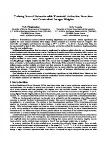
Artificial Neural Networks are computational models naturally performing a parallel processing of information [10]. Essentially, an ANN can be defined as a pool of simple processing units (neurons) which communicate among themselves by means of sending analog signals. These signals travel through weighted connections between neurons. Each of these neurons accumulates the inputs it receives, producing an output according to an internal activation function. This output can serve as an input for other neurons, or can be a part of the network output. In Fig. 1 left we can see a neuron in detail.
Output
Inputs A1 A2 A3
AN q Bias
Weights W1
Output Layer
W2
Neuron
W3 Sum-of-Product
WN 1
G
x Sumation Function
Output
f(x) Activation Function
y
Hidden Layer Connection weights Input Layer
Input Pattern
Fig. 1. An artificial neuron (left) and a multilayer perceptron (right)
There is a set of important issues involved in the ANN design process. As a first step, the architecture of the network has to be decided. Initially, two major options are usually considered: feedforward networks and recurrent networks (additional considerations regarding the order of the ANN exist, but are out of our scope). The feedforward model comprises networks in which the connections are strictly feedforward, i.e., no neuron receives input from a neuron to which the former sends its output, even indirectly. The recurrent model defines networks in which feedback connections are allowed, thus making the dynamical properties of a capital importance. In this work we will concentrate on the first and simpler model: the feedforward networks. To be precise, we will consider the so-called multilayer perceptron (MLP) [11], in which units are structured into ordered layers, and connections are allowed only between adjacent layers in an input-to-output sense (see Fig. 1 right). For any MLP, several parameters such as the number of layers and the number of units per layer must be defined. After having done this, the last step in the design is to adjust the weights of the network, so that it produces the desired output when the corresponding input is presented. This process is known as training the ANN or learning the network weights. Network weights comprise both the previously mentioned connection weights, as well as a bias term for each unit. The latter can be viewed as the weight of a constant saturated input that the corresponding unit always receives. As initially stated, we will focus on the learning situation known as supervised training, in which a set of input/desired-output patterns is available. Thus, the ANN has to be trained to produce the desired output according to these examples. The input and output of the network are both real vectors in our case. In order to perform a supervised training we need a way of evaluating the ANN output error between the actual and the expected output. A popular measure is the Squared Error Percentage (SEP). We can compute this error term just for one single pattern or for a set of patterns. In this last case, the SEP is the average value of the patterns individual SEP. The expression for this global SEP is:
SEP = 100 ·
P S omax − omin X X p (ti − opi )2 . P ·S p=1 i=1
(1)
where tpi and opi are, respectively, the i-th components of the expected vector and the actual current output vector for the pattern p; omin and omax are the minimum and maximum values of the output neurons, S is the number of output neurons, and P is the number of patterns. In classification problems, we could use still an additional measure: the Classification Error Percentage (CEP). CEP is the percentage of incorrectly classified patterns, and it is a usual complement to any of the other two (SEP or the wellknown MSE) raw error values, since CEP reports in a high-level manner the quality of the trained ANN.
3
The Algorithms
We use for our study several algorithms to train ANNs: the Backpropagation algorithm, the Levenberg-Marquardt algorithm, a Genetic Algorithm, a hybrid between Genetic Algorithm and Backpropagation, and a hybrid between Genetic Algorithm and Levenberg-Marquardt. We briefly describe them in the following paragraphs. 3.1
Backpropagation
The Backpropagation algorithm (BP) [2] is a classical domain-dependent technique for supervised training. It works by measuring the output error, calculating the gradient of this error, and adjusting the ANN weights (and biases) in the descending gradient direction. Hence, BP is a gradient-descent local search procedure (expected to stagnate in local optima in complex landscapes). First, we define the squared error of the ANN for a set of patterns: E=
S P X X
(tpi − opi )2 .
(2)
p=1 i=1
The actual value of the previous expression depends on the weights of the network. The basic BP algorithm (without momentum in our case) calculates the gradient of E (for all the patterns in our case) and updates the weights by moving them along the gradient-descendent direction. This can be summarized with the expression ∆w = −η∇E, where the parameter η > 0 is the learning rate that controls the learning speed. The pseudo-code of the BP algorithm is shown in Fig. 2.
InitializeWeights; while not StopCriterion do for all i,j do ∂E wij := wij − η ∂w ; ij endfor; endwhile; Fig. 2. Pseudo-code of the BP algorithm
3.2
Levenberg-Marquardt
The Levenberg-Marquardt algorithm (LM) [9] is an approximation to the Newton method used also for training ANNs. The Newton method approximates the error of the network with a second order expression, which contrasts to the Backpropagation algorithm that does it with a first order expression. LM is popular in the ANN domain (even it is considered the first approach for an unseen
MLP training task), although it is not that popular in the metaheuristics field. LM updates the ANN weights as follows: "
∆w = − µI +
P X p=1
p
T
p
J (w) J (w)
#−1
∇E(w) .
(3)
where J p (w) is the Jacobian matrix of the error vector ep (w) evaluated in w, and I is the identity matrix. The vector error ep (w) is the error of the network for pattern p, that is, ep (w) = tp −op (w). The parameter µ is increased or decreased at each step. If the error is reduced, then µ is divided by a factor β, and it is multiplied by β in other case. Levenberg-Marquardt performs the steps detailed in Fig. 3. It calculates the network output, the error vectors, and the Jacobian matrix for each pattern. Then, it computes ∆w using (3) and recalculates the error with w + ∆w as network weights. If the error has decreased, µ is divided by β, the new weights are maintained, and the process starts again; otherwise, µ is multiplied by β, ∆w is calculated with a new value, and it iterates again.
InitializeWeights; while not StopCriterion do Calculates ep (w) for each pattern; PP e1 := ep (w)T ep (w); p=1 Calculates J p (w) for each pattern; repeat Calculates ∆w; PP e2 := ep (w + ∆w)T ep (w + ∆w); p=1 if (e1