Nov 17, 2017 - gradients and update all model parameters in each learning step. It is not uncommon for a ... only speed up the training of the neural networks. One of the ...... means applying model compression on top of meProp. h = 500 means ..... focusing on reducing the communication cost in distributed systems ([10] ...
1
Training Simplification and Model Simplification for Deep Learning: A Minimal Effort Back Propagation Method arXiv:1711.06528v1 [cs.LG] 17 Nov 2017
Xu Sun, Xuancheng Ren, Shuming Ma, Bingzhen Wei, Wei Li, and Houfeng Wang Abstract—We propose a simple yet effective technique to simplify the training and the resulting model of neural networks. In back propagation, only a small subset of the full gradient is computed to update the model parameters. The gradient vectors are sparsified in such a way that only the top-k elements (in terms of magnitude) are kept. As a result, only k rows or columns (depending on the layout) of the weight matrix are modified, leading to a linear reduction in the computational cost. Based on the sparsified gradients, we further simplify the model by eliminating the rows or columns that are seldom updated, which will reduce the computational cost both in the training and decoding, and potentially accelerate decoding in real-world applications. Surprisingly, experimental results demonstrate that most of time we only need to update fewer than 5% of the weights at each back propagation pass. More interestingly, the accuracy of the resulting models is actually improved rather than degraded, and a detailed analysis is given. The model simplification results show that we could adaptively simplify the model which could often be reduced by around 9x, without any loss on accuracy or even with improved accuracy. Index Terms—neural network, back propagation, sparse learning, model pruning.
✦
1
I NTRODUCTION
N
EURAL network learning is typically slow, where back propagation usually dominates the computational cost during the learning process. Back propagation entails a high computational cost because it needs to compute full gradients and update all model parameters in each learning step. It is not uncommon for a neural network to have a massive number of model parameters. In this study, we propose a minimal effort back propagation method, which we call meProp, for neural network learning. The idea is that we compute only a very small but critical portion of the gradient information, and update only the corresponding minimal portion of the parameters in each learning step. This leads to sparsified gradients, such that only highly relevant parameters are updated, while other parameters stay untouched. The sparsified back propagation leads to a linear reduction in the computational cost. On top of meProp, we further propose to simplify the trained model by eliminating the less relevant parameters discovered during meProp, so that the computational cost of decoding can also be reduced. We name the method meSimp (minimal effort simplification). The idea is that we record which portion of the parameters is updated at each learning step in meProp, and gradually remove the parameters that are less updated. This leads to a simplified model that costs
•
X. Sun, X. Ren, S. Ma, B. Wei, W. Li, and H. Wang are with School of Electronics Engineering and Computer Science, Peking University, China, and MOE Key Laboratory of Computational Linguistics, Peking University, China. E-mail: {xusun, renxc, shumingma, weibz, liweitj47, wanghf}@pku.edu.cn
The first two authors contributed equally to this work. This work is a substantial extension of the work presented at ICML 2017 [1]. The codes are available at https://github.com/jklj077/meProp.
less in computation during decoding, while meProp can only speed up the training of the neural networks. One of the motivations for such method is that if we suppose back propagation can determine the importance of input features, with meProp, the essential features are welltrained, and the non-essential features are less-trained, so that the robustness of the models can be improved, and overfitting can be reduced. As the essential features play a more important role in the final model, there are chances that the parameters related to non-essential features could be eliminated, which leads to the idea of meSimp. For a classification task, there are essential features that are decisive in the classification, non-essential features that are helpful but can also be distractions, and irrelevant features that are not useful at all. For example, when classifying a picture as a taxi, the taxi sign is one of the essential features, and the color yellow, which is often the color of a taxi, is one of the non-essential features. Overfitting often occurs when the non-essential features are given too much importance in the model, while meProp intentionally focuses on training the probable essential features to lessen the risk of overfitting. To realize our approaches, we need to answer four questions. The first question is how to find the highly relevant subset of the parameters from the current sample in stochastic learning. We propose a top-k search method to find the most important parameters. Interestingly, experimental results demonstrate that most of the time we only need to update fewer than 5% of the weights at each back propagation pass. This does not result in a larger number of training iterations. The proposed method is general-purpose and it is independent of specific models and specific optimizers (e.g., Adam and AdaGrad). The second question is whether or not this minimal effort
2
Fig. 1. An illustration of meProp.
back propagation strategy would hurt the accuracy of the trained models. We show that our strategy does not degrade the accuracy of the trained model, even when a very small portion of the parameters is updated. More interestingly, our experimental results reveal that our strategy actually improves the model accuracy in most cases. Based on our experiments, we find that it is probably because the minimal effort update does not modify weakly relevant parameters in each update, according with our assumption, which makes overfitting less likely, similar to the dropout effect. The third question is whether or not the decoding cost of the model can be reduced, as meProp can only shorten the training time. Based on meProp, we further apply the technique of meSimp. From our observations, the simplifying strategy can indeed shrink the final model by usually around 9x without any loss on accuracy. It also supports our assumption that, in fact, many learned features are not essential to the final correct prediction. The final question is whether or not the size of the simplified models needs to be set explicitly in advance. In most previous work, the final model size is pre-configured as desired or using heuristic rules, making it hard to simplify models with multiple layers, because naturally, each layer should have a different dimension, since it captures a different level of abstraction. In practice, we find that meSimp could adaptively reduce the size of the hidden layers, and automatically decide which features are essential for the task at different abstraction levels, resulting in a model of different hidden layer sizes. The contributions of this work are as follows: •
•
We propose a minimal effort back propagation technique for neural network learning, which could automatically find the most important features. Only a small subset of the full gradient is computed to update the model parameters, and is used to determine whether the related parameters should be kept in the final model. Applying the technique to training simplification (meProp), we find that the strategy actually improve the accuracy of the resulting models, rather than degraded, even if fewer than 5% of the weights are updated at each back propagation pass most of the time. The technique does not entail a larger number
•
•
2
of training iterations, and could reduce the time of the training substantially. Most importantly, applying the technique to model simplification (meSimp) could potentially reduce the time of decoding. With the ability to adaptively simplify each layer of the model to only keep essential features, the resulting model could be reduced to around one ninth of its original size, which equals to an around 9x reduction in decoding cost, on a base of no accuracy loss or even improved accuracy. It’s worth mentioning, when applied to models with multiple layers, given a single hyper-parameter, meSimp could simplify each hidden layer to a different extent, alleviating the need to set different hyperparameters for different layers. The minimal effort back propagation technique can be applied to different types of deep learning models (MLP and LSTM), can be applied with various optimization methods (Adam and AdaGrad), and works on diverse tasks (natural language processing and image recognition).
P ROPOSED M ETHOD
We propose a simple yet effective technique for neural network learning. The forward propagation is computed as usual. During back propagation, only a small subset of the full gradient is computed to update the model parameters. The gradient vectors are “quantized” so that only the topk components in terms of magnitude are kept. Based on the technique, we further propose to simplify the resulting models by removing the rows that are seldom updated, according to the top-k indices. The model is simplified in such a way that only actively updated rows are kept. We first present the proposed methods, and then describe the implementation details. 2.1 Simplified Back Propagation (meProp) Forward propagation of neural network models, including feedforward neural networks, RNN, LSTM, consists of linear transformations and non-linear transformations. For simplicity, we take a computation unit with one linear transformation and one non-linear transformation as an example:
y = Wx
(1)
3
Fig. 2. An illustration of the computational flow of meProp.
z = σ(y)
(2)
where W ∈ Rn×m , x ∈ Rm , y ∈ Rn , z ∈ Rn , m is the dimension of the input vector, n is the dimension of the output vector, and σ is a non-linear function (e.g., relu, tanh, and sigmoid). During back propagation, we need to compute the gradient of the parameter matrix W and the input vector x: ′ ∂z = σi xTj (1 ≤ i ≤ n, 1 ≤ j ≤ m) (3) ∂Wij
X ′ ∂z WijT σj (1 ≤ j ≤ n, 1 ≤ i ≤ m) = ∂xi j
(4)
′
∂zi . We can see that the computawhere σi ∈ Rn means ∂y i tional cost of back propagation is directly proportional to the dimension of output vector n. The proposed meProp uses approximate gradients by keeping only top-k elements based on the magnitude values. That is, only the top-k elements with the largest absolute values are kept. For example, suppose a vector v = h1, 2, 3, −4i, then top2 (v) = h0, 0, 3, −4i. We de′ note the indices of vector σ (y)’s top-k values as S = {t1 , t2 , ..., tk }(1 ≤ k ≤ n), and the approximate gradient of the parameter matrix W and input vector x is: ′ ∂z ← σi xTj if i ∈ {t1 , t2 , ..., tk } else 0 ∂Wij
(5)
X ′ ∂z WijT σj if j ∈ {t1 , t2 , ..., tk } else 0 ← ∂xi j
(6)
As a result, only k rows or columns (depending on the layout) of the weight matrix are modified, leading to a linear reduction (k divided by the vector dimension) in the computational cost. The algorithm is described in Algorithm 1. Figure 1 is an illustration of meProp for a single computation unit of neural models. The original back propagation uses the full gradient of the output vectors to compute the gradient of the parameters. The proposed method selects the top-k values of the gradient of the output vector, and back propagates the loss through the corresponding subset of the total model parameters. Algorithm 1 Backward Propagation Simplification for A Computation Unit
z ← σ(W x) ⊲ Forward propagation ′ ∂z ⊲ Gradient of W x w.r.t. z σ ← ∂σ S ← {t1 , t2 , ..., tk } ⊲ Indices of k largest derivatives of ′ σ in magnitude ′ ∂z ← σi xTj if i ∈ S else 0 4: ∂W ij P ∂z T ′ 5: ∂x ← j Wij σj if j ∈ S else 0 i
1: 2: 3:
As for a complete neural network framework with a loss L, the original back propagation computes the gradient of the parameter matrix W as:
∂L ∂y ∂L = · ∂W ∂y ∂W
(7)
4
Fig. 3. An illustration of the computational flow of meProp on a mini-batch learning setting.
while the gradient of the input vector x is:
∂y ∂L ∂L = · ∂x ∂x ∂y
(8)
The proposed meProp selects top-k elements of the gradient ∂L ∂y to approximate the original gradient, and passes them through the gradient computation graph according to the chain rule. Hence, the gradient of W goes to:
∂L ∂L ∂y ← topk ( )· ∂W ∂y ∂W
(9)
while the gradient of the vector x is:
∂y ∂L ∂L ← · topk ( ) ∂x ∂x ∂y
(10)
Figure 2 shows an illustration of the computational flow of meProp. The forward propagation is the same as traditional forward propagation, which computes the output vector via a matrix multiplication operation between two input tensors. The original back propagation computes the full gradient for the input vector and the weight matrix. For meProp, back propagation computes an approximate gradient by keeping top-k values of the backward flowed gradient and masking the remaining values to 0. Figure 3 further shows the computational flow of meProp for the mini-batch case. 2.2 Simplified Model (meSimp) The method from section 2.1 simplifies the training process, thus reduces the training time. However, for most deep
learning applications in real life, it is even more important to reduce the computational cost of decoding, for the fact that although training is time consuming, it only needs to be done once, while decoding needs to be done as long as there is a new request. In this section, we propose to simplify the model by eliminating the inactive paths, which we define as the neurons whose gradients are not in top-k . This way, the decoding cost would also be reduced. There are two major concerns about this proposal. The main problem here is that we don’t know the active path of unseen examples in advance, as we don’t know the gradient information of those examples. Our solution for this problem is that we could obtain the overall inactive paths from the inactive paths of the training samples, which could be removed gradually in the training. The second is that the reduction in dimension could lead to performance degradation. Surprisingly, from our experimental results, our top-k gradient based method does not deteriorate the model. Instead, with an appropriate configuration, the resulting smaller model often performs better than the baseline large model, or even the baseline model of the similar size. As a matter of fact, after pruning the performance does drop. However, with the following training, the performance is regained. In what follows, we will briefly introduce the inspiration of the proposed method, and how the model simplification is done. In the experiments of meProp, we discover an interesting phenomenon that during training, apart from the active paths with top-k gradients, there are some inactive paths that are not activated at all for any of the examples. We call
5
these paths universal inactive paths. These neurons are not updated at all during training, and their parameter values remain the same as their initialized values, and we have every reason to believe that they would not be effective for new samples as well. However, the number of those paths may not be enough to bring a substantial contraction to the model. Algorithm 2 Model Simplification for A Computation Unit 1: Initialize W , t ← 0, c ← 0 2: while training do 3: Draw (x, y) from training data 4: z ← σ(W x) ⊲ Forward propagation ′ ∂z T ⊲ Gradient of W w.r.t. z 5: ∂W ← topk (σ )x 6: S ← {t1 , t2 , ..., tk } ⊲ indices of k largest derivatives ′ of σ in magnitude 7: ci ← increase if i in S ⊲ Record the top-k indices ∂z 8: Update W with ∂W 9: if t mod m = 0 then ⊲ Prune inactive paths 10: θ ← m × prune rate 11: for all i where ci < θ do 12: Remove row i from W 13: end for 14: c←0 ⊲ Reset c 15: end if 16: t←t+1 17: end while Based on the previous findings, we generalize the idea of universal inactive paths, and prune the paths that are less updated, that is, the paths we eliminate are the paths that are not active for a number of samples. To realize the idea, we keep a record c of how many times the index is in the top-k indices S , during the back propagation at the same time as meProp. After several training steps m, we take out the less active paths that are not updated for a number of samples, e.g. 90% prune rate, which results in a simplified model. The record is cleared at each pruning action. By doing that iteratively, the model size will approach near stable in the end. Algorithm 2 describes the method for a computation unit, and an illustration is shown in Figure 4. An important hyper-parameter for the method is the pruning threshold. When determining the threshold, the model size and the number of examples between pruning actions should be taken into account. As shown in Algorithm 2, the threshold could be parameterized by prune interval, that is, how many samples between pruning, and prune rate, that is, how active the path should be if it is not to be eliminated. Note that the layer sizes are determined adaptively in a multi-layer setting, and only one threshold is needed for a model with multiple layers to have different layer sizes. Because the top-k indices of different layers at different iterations intersect differently in back propagation. For some layers, the top-k indices are similar, hence results in a larger layer size, compared to k . For other layers, the top-k indices are quite different at each iteration, so that the intersection happens more often, which means ci is lower, hence the resulting layer size is smaller. How the layer is simplified depends on how the learning is done, which is in accordance with our intuition.
forward propaga!on (original)
back propaga!on (meProp)
model simplifica!on
ac!veness collected from mul!ple examples
forward propaga!on (simplified)
inac!ve neurons are eliminated
back propaga!on (simplified & meProp)
Fig. 4. An illustration of model simplification (k = 2). The figure shows the three main stages of the simplified model training. First, as the upper shows, the model is trained using meProp, for several iterations, and a record of the “activeness” of the paths is kept, indicated by the shades of the neurons. Second, as the middle shows, the model is simplified based on the collected record, and the inactive paths are eliminated. Third, as the lower shows, we train the simplified model also using meProp. We repeat the procedure until the goal of the training is met.
In a deep neural network, it’s worth noticing that when simplifying a hidden layer, the respective columns in the “next” layer could also be removed, as the values in the columns represent the connection between the eliminated inputs and the outputs, which is no longer effective. That could reduce the model even further. However, we have not include that in our implementation yet. There are some extra considerations for LSTM models. In an LSTM, there is a lasting linear memory, and four gates controlling the modifying of the memory cells. It makes sense only if the pruning is for the memory cells instead of the gates, which are the computation units defined previously, because there is coherence between the memory and
6
the gates. Otherwise, the pruning would cause chaos and mismatch of dimensions, as each gate is of its own size, and the memory is of another dimension if it is set to the union of the gates. For LSTM models, we treat an LSTM module as a whole unit for model simplification, instead of treating each gate in an LSTM module as a unit for simplification. However, the top-k gradient selection takes place as the level of gates rather than memory cells. In practice, we still obtain the top-k indices from the gates, but we merge the top-k indices records of the gates into one record, and the pruning is for memory cells, so that the related gates are pruned as well. For model simplification, we also propose a kind of cycle mechanism. During our experiments, we find that at the time of the simplification, there is a drop in performance, but it recovers quickly within the following training, and may even supersede the performance before the simplification. It makes us wonder whether the training after simplification is critical to the performance improvement. We propose to divide the training procedure into several stages, and in each stage, we first conduct the training of model simplification, and then conduct the normal training. At the start of each stage, we also reinitialize the optimizer, if there is historical information of the gradients stored. The reason for such operation is that after model simplification, the dynamics of how the neurons interacted with each other changed, and the previous gradient information may interfere with the new dynamics of the simplified network. We find this cycle mechanism could improve the resulting model’s performance even further on some tasks. 2.3 Implementation We have coded two neural network models, including an LSTM model for part-of-speech (POS) tagging, and a feedforward NN model (MLP) for transition-based dependency parsing and MNIST image recognition. We use the optimizers with automatically adaptive learning rates, including Adam [2] and AdaGrad [3]. In our implementation, we make no modification to the optimizers, although there are many zero elements in the gradients. Most of the experiments on CPU are conducted on the framework coded in C# on our own. This framework builds a dynamic computation graph of the model for each sample, making it suitable for data in variable lengths. A typical training procedure contains three parts: forward propagation, back propagation, and parameter update. We also have an implementation based on the PyTorch framework for GPU based experiments. To focus on the method itself, the results of GPU based experiments will be presented in appendices. 2.3.1 Where to apply top-k selection The proposed method aims to reduce the complexity of the back propagation by reducing the elements in the computationally intensive operations. In our preliminary observations, matrix-matrix or matrix-vector multiplication consumed more than 90% of the time of back propagation. In our implementation, we apply meProp only to the back propagation from the output of the multiplication to its inputs. For other element-wise operations (e.g., activation
functions), the original back propagation procedure is kept, because those operations are already fast enough compared with matrix-matrix or matrix-vector multiplication operations. If there are multiple hidden layers, the top-k sparsification needs to be applied to every hidden layer, because the sparsified gradient will again be dense from one layer to another. That is, in meProp the gradients are sparsified with a top-k operation at the output of every hidden layer. While we apply meProp to all hidden layers using the same k of top-k , usually the k for the output layer could be different from the k for the hidden layers, because the output layer typically has a very different dimension compared with the hidden layers. For example, there are 10 tags in the MNIST task, so the dimension of the output layer is 10, and we use an MLP with the hidden dimension of 500. Thus, the best k for the output layer could be different from that of the hidden layers. 2.3.2 Choice of top-k algorithms In our C# implementation, instead of sorting the entire vector, we use the well-known min-heap based top-k selection method, which is slightly changed to focus on memory reuse. The algorithm has a time complexity of O(n log k) and a space complexity of O(k). PyTorch comes with a GPU implementation of a certain paralleled top-k algorithm, which we are not sure how the operation is done exactly.
3
E XPERIMENTS
To demonstrate that the proposed method is generalpurpose, we perform experiments on different models (LSTM/MLP), various training methods (Adam/AdaGrad), and diverse tasks. Transition-based Dependency Parsing (Parsing): Following prior work, we use English Penn TreeBank (PTB) [4] for evaluation. We follow the standard split of the corpus and use sections 2-21 as the training set (39,832 sentences, 1,900,056 transition examples),1 section 22 as the development set (1,700 sentences, 80,234 transition examples) and section 23 as the final test set (2,416 sentences, 113,368 transition examples). The evaluation metric is unlabeled attachment score (UAS). We implement a parser using MLP following [5], which is used as our baseline. Part-of-Speech Tagging (POS-Tag): We use the standard benchmark dataset in prior work [6], which is derived from the Penn Treebank corpus, and use sections 0-18 of the Wall Street Journal (WSJ) for training (38,219 examples), and sections 22-24 for testing (5,462 examples). The evaluation metric is per-word accuracy. A popular model for this task is the LSTM model [7],2 which is used as our baseline. MNIST Image Recognition (MNIST): We use the MNIST handwritten digit dataset [8] for evaluation. MNIST consists of 60,000 28×28 pixel training images and additional 10,000 test examples. Each image contains a single numerical digit (0-9). We select the first 5,000 images of the training images as the development set and the rest as the 1. A transition example consists of a parsing context and its optimal transition action. 2. In this work, we use the bi-directional LSTM (Bi-LSTM) as the implementation of LSTM.
7
TABLE 1 meProp results based on LSTM/MLP models and Adam optimizers. Time means averaged time per iteration. Iter means the number of iterations to reach the optimal score on development data. The model of this iteration is then used to obtain the test score. As we can see, applying meProp can substantially speedup the back propagation with improved accuracy. Parsing (Adam) MLP (h=500) meProp (k=20) POS-Tag (Adam) LSTM (h=500) meProp (k=10) MNIST (Adam) MLP (h=500) meProp (k=80)
Iter 10 6 Iter 3 4 Iter 13 14
Backprop time (s) 9,077.7 488.7 (18.6x) Backprop time (s) 16,167.3 435.6 (37.1x) Backprop time (s) 169.5 28.7 ( 5.9x)
training set. The evaluation metric is per-image accuracy. We use the MLP model as the baseline. Following common practice, we use ReLU [9] as the activation function of the hidden layers. 3.1 Experimental Settings We set the dimension of the hidden layers to 500 for all the tasks. For Parsing, the input dimension is 48 (features) × 50 (dim per feature) = 2400, and the output dimension is 25. For POS-Tag, the input dimension is 1 (word) × 50 (dim per word) + 7 (features) × 20 (dim per feature) = 190, and the output dimension is 45. For MNIST, the input dimension is 28 (pixels per row) × 28 (pixels per column) × 1 (dim per pixel) = 784, and the output dimension is 10. Based on the development set and prior work, we set the mini-batch size to 10,000 (transition examples), 1 (sentence), and 10 (images) for Parsing, POS-Tag, and MNIST, respectively. Using 10,000 transition examples for Parsing follows [5]. As discussed in Section 2, the optimal k of topk for the output layer could be different from the hidden layers, because their dimensions could be very different. For Parsing and MNIST, we find using the same k for the output and the hidden layers works well, and we simply do so. For another task, POS-Tag, we find the the output layer should use a different k from the hidden layers. For simplicity, we do not apply meProp to the output layer for POS-Tag, because in this task we find the computational cost of the output layer is almost negligible compared with other layers. In the experiments of model simplification, we use the Adam optimizer for all the tasks, for the sake of simplicity. In addition, we also apply the cycle mechanism in the reported results. Note that, to simulate the real scenario, we run each configuration 5 times with different random seeds, and choose the best model on development set to report. The hyperparameters are tuned based on the development data. For the Adam optimization method, we find the default hyperparameters work well on development sets, which are as follows: the learning rate α = 0.001, and β1 = 0.9, β2 = 0.999, ǫ = 1 × 10⁻⁸ . The experiments on CPU are conducted on a computer with the INTEL(R) Xeon(R) 3.0GHz CPU. The experiments on GPU are conducted on NVIDIA GeForce GTX 1080. 3.2 Experimental Results of meProp In this experiment, the LSTM is based on one hidden layer and the MLP is based on two hidden layers (experiments
Dev UAS (%) 90.48 89.91 Dev Acc (%) 97.20 97.14 Dev Acc (%) 98.72 98.36
Test UAS (%) 89.80 89.84 (+0.04) Test Acc (%) 97.22 97.25 (+0.03) Test Acc (%) 98.20 98.27 (+0.07)
on more hidden layers will be presented later). We conduct experiments on different optimization methods, including AdaGrad and Adam. Since meProp is applied to the linear transformations (which entail the major computational cost), we report the linear transformation related backprop time as Backprop Time. It does not include non-linear activations, which usually have only less than 2% computational cost. The total time of back propagation, including nonlinear activations, is reported as Overall Backprop Time. Table 1 shows the results based on different models and different optimization methods. In the table, meProp means applying meProp to the corresponding baseline model, h = 500 means that the hidden layer dimension is 500, and k = 20 means that meProp uses top-20 elements (among 500 in total) for back propagation. Note that, for fair comparisons, all experiments are first conducted on the development data and the test data is not observable. Then, the optimal number of iterations is decided based on the optimal score on development data, and the model of this iteration is used upon the test data to obtain the test scores. As we can see, applying meProp can substantially speed up the back propagation. It provides a linear reduction in the computational cost. Surprisingly, results demonstrate that we can update only fewer than 5% of the weights at each back propagation pass for the natural language processing tasks. This does not result in a larger number of training iterations. More surprisingly, the accuracy of the resulting models is actually improved rather than decreased. The main reason could be that the minimal effort update does not modify weakly relevant parameters, which makes overfitting less likely, similar to the dropout effect. 3.2.1 Result Analysis of meProp Changing Optimizer TABLE 2 meProp: Results using AdaGrad optimizers. We can see that meProp also works with AdaGrad optimizers, indicating that meProp is independent of optimizers. Parsing (AdaGrad) MLP (h=500) meProp (k=20) POS-Tag (AdaGrad) LSTM (h=500) meProp (k=5) MNIST (AdaGrad) MLP (h=500) meProp (k=10)
Iter 11 8 Iter 4 4 Iter 8 16
Test UAS (%) 88.92 88.95 (+0.03) Test Acc (%) 96.93 97.25 (+0.32) Test Acc (%) 97.52 98.00 (+0.48)
8
100
98 97.9 97.8
97.6 0
meProp MLP 20
40 60 80 Backprop Ratio (%)
100
98
98
97
96
96
Accuracy (%)
Accuracy (%)
Accuracy (%)
98.1
97.7
MNIST: Change h/k
MNIST: Topk vs Random
MNIST: Reduce Overfitting 98.2
94 92 90 Topk meProp Random meProp
88 86 0
5 10 Backprop Ratio (%)
95 94 93 92 0
15
meProp MLP
91
2 4 6 8 Backprop/Hidden Ratio (%)
10
Fig. 5. Accuracy vs. meProp’s backprop ratio (left). Results of top-k meProp vs. random meProp (middle). Results of top-k meProp vs. baseline with the hidden dimension h (right). TABLE 3 meProp: Results based on the same k and h. It can be concluded that meProp does not rely on redundant neurons, as the model of the small hidden dimension works much worse. Parsing (Adam) MLP (h=20) meProp (k=20) POS-Tag (Adam) LSTM (h=5) meProp (k=5) MNIST (Adam) MLP (h=20) meProp (k=20)
Iter 18 6 Iter 7 5 Iter 15 17
Test UAS (%) 88.37 90.01 (+1.64) Test Acc (%) 96.40 97.12 (+0.72) Test Acc (%) 95.77 98.01 (+2.24)
It is important to see whether meProp can be applied with different optimizers, because the minimal effort technique sparifies the gradient, which affects the update of the parameters. For the AdaGrad learner, the learning rate is set to α = 0.01, 0.01, 0.1 for Parsing, POS-Tag, and MNIST, respectively, and ǫ = 1 × 10⁻⁶ . As shown in Table 2, the results are consistent among AdaGrad and Adam. The results demonstrate that meProp is independent of specific optimization methods. For simplicity, the following experiments use Adam. Varying Backprop Ratio In Figure 5 (left), we vary the k of top-k meProp to compare the test accuracy on different ratios of meProp backprop. For example, when k=5, it means that the backprop ratio is 5/500=1%. The optimizer is Adam. As we can see, meProp achieves consistently better accuracy than the baseline. Top-k vs. Random It will be interesting to check the role of top-k elements. Figure 5 (middle) shows the results of top-k meProp vs. random meProp. The random meProp means that random elements (instead of top-k ones) are selected for back propagation. As we can see, the top-k version works better than the random version. It suggests that top-k elements contain the most important information of the gradients. Varying Hidden Dimension We still have a question: does the top-k meProp work well simply because the original model does not require that big dimension of the hidden layers? For example, the meProp (topk=5) works simply because the LSTM works well with the hidden dimension of 5, and there is no need
TABLE 4 meProp: Varying the number of hidden layers on the MNIST task. The experiments demonstrate that meProp can also be applied to traditional deep models. Layers 2 3 4 5
Method MLP (h=500) meProp (k=25) MLP (h=500) meProp (k=25) MLP (h=500) meProp (k=25) MLP (h=500) meProp (k=25)
Test Acc (%) 98.10 98.20 (+0.10) 98.21 98.37 (+0.16) 98.10 98.15 (+0.05) 98.05 98.21 (+0.16)
to use the hidden dimension of 500. To examine this, we perform experiments on using the same hidden dimension as k , and the results are shown in Table 3. As we can see, however, the results of the small hidden dimensions are much worse than those of meProp. In addition, Figure 5 (right) shows more detailed curves by varying the value of k . In the figure, different k gives different backprop ratio for meProp and different hidden dimension ratio for LSTM/MLP. As we can see, the answer to that question is negative: meProp does not rely on redundant hidden layer elements. Adding More Hidden Layers Another question is whether or not meProp relies on shallow models with only a few hidden layers. To answer this question, we also perform experiments on more hidden layers, from 2 hidden layers to 5 hidden layers. We find setting the dropout rate to 0.1 works well for most cases of different numbers of layers. For simplicity of comparison, we set the same dropout rate to 0.1 in this experiment. Table 4 shows that adding the number of hidden layers does not hurt the performance of meProp. Adding Dropout Since we have observed that meProp can reduce overfitting of deep learning, a natural question is that if meProp is reducing the same type of overfitting risk as dropout. Thus, we use development data to find a proper value of the dropout rate on those tasks, and then further add meProp to check if further improvement is possible. Table 5 shows the results. As we can see, meProp can achieve further improvement over dropout. In particular, meProp has an improvement of 0.46 UAS on Parsing. The results suggest that the type of overfitting that meProp
9
TABLE 5 meProp: Adding the dropout technique. As the results show, meProp could further improve the performance on top of dropout, suggesting that meProp is reducing a different type of overfitting, comparing to dropout. Parsing (Adam) MLP (h=500) meProp (k=40) POS-Tag (Adam) LSTM (h=500) meProp (k=20) MNIST (Adam) MLP (h=500) meProp (k=25)
Dropout 0.5 0.5 Dropout 0.5 0.5 Dropout 0.2 0.2
Test UAS (%) 91.53 91.99 (+0.46) Test Acc (%) 97.20 97.31 (+0.11) Test Acc (%) 98.09 98.32 (+0.23)
TABLE 6 Results of simple unified top-k meProp based on a whole mini-batch (i.e., unified sparse patterns). The optimizer is Adam. Mini-batch Size is 50. Layers 2 5
Method MLP (h=500) meProp (k=30) MLP (h=500) meProp (k=50)
Test Acc (%) 97.97 98.08 (+0.11) 98.09 98.36 (+0.27)
reduces is probably different from that of dropout. Thus, a model should be able to take advantage of both meProp and dropout to reduce overfitting. Speedup on GPU For implementing meProp on GPU, the simplest solution is to treat the entire mini-batch as a “big training example”, where the top-k operation is based on the averaged values of all examples in the mini-batch. In this way, the big sparse matrix of the mini-batch will have consistent sparse patterns among examples, and this consistent sparse matrix can be transformed into a small dense matrix by removing the zero values. We call this implementation as simple unified top-k . This experiment is based on PyTorch. Despite its simplicity, Table 6 shows the good performance of this implementation, which is based on the minibatch size of 50. We also find the speedup on GPU is less significant when the hidden dimension is low. The reason is that our GPU’s computational power is not fully consumed by the baseline (with small hidden layers), so that the normal back propagation is already fast enough, making it hard for meProp to achieve substantial speedup. For example, supposing a GPU can finish 1000 operations in one cycle, there could be no speed difference between a method with 100 and a method with 10 operations. Indeed, we find MLP (h=64) and MLP (h=512) have almost the same GPU speed even on forward propagation (i.e., without meProp), while theoretically there should be an 8x difference. With GPU, the forward propagation time of MLP (h=64) and MLP (h=512) is 572ms and 644ms, respectively. This provides evidence for our hypothesis that our GPU is not fully consumed with the small hidden dimensions. Thus, the speedup test on GPU is more meaningful for the heavy models, such that the baseline can at least fully consume the GPU’s computational power. To check this, we test the GPU speedup on synthetic data of matrix multiplication with a larger hidden dimension. Indeed, Table 7 shows that meProp achieves much higher speed than
TABLE 7 Acceleration results on the matrix multiplication synthetic data using GPU. The batch size is 1024. Method Baseline (h=8192) meProp (k=8) meProp (k=16) meProp (k=32) meProp (k=64) meProp (k=128) meProp (k=256) meProp (k=512)
Backprop time (ms) 308.00 8.37 (36.8x) 9.16 (33.6x) 11.20 (27.5x) 14.38 (21.4x) 21.28 (14.5x) 38.57 ( 8.0x) 69.95 ( 4.4x)
TABLE 8 Acceleration results on MNIST using GPU. Method MLP (h=8192) meProp (k=8) meProp (k=16) meProp (k=32) meProp (k=64) meProp (k=128) meProp (k=256) meProp (k=512)
Overall backprop time (ms) 17,696.2 1,501.5 (11.8x) 1,542.8 (11.5x) 1,656.9 (10.7x) 1,828.3 ( 9.7x) 2,200.0 ( 8.0x) 3,149.6 ( 5.6x) 4,874.1 ( 3.6x)
the traditional backprop with the large hidden dimension. Furthermore, we test the GPU speedup on MLP with the large hidden dimension [10]. Table 8 shows that meProp also has substantial GPU speedup on MNIST with the large hidden dimension. In this experiment, the speedup is based on Overall Backprop Time (see the prior definition). Those results demonstrate that meProp can achieve good speedup on GPU when it is applied to heavy models. Finally, there are potentially other implementation choices of meProp on GPU. For example, another natural solution is to use a big sparse matrix to represent the sparsified gradient of the output of a mini-batch. Then, the sparse matrix multiplication library can be used to accelerate the computation. This could be an interesting direction of future work. 3.3 Experimental Results of meSimp In this experiment, we only simplify the hidden layers of the model, and we use Adam optimizer for all the tasks. We set the cycle to 10 for all the tasks, that is, we first train the model using meSimp for 5 epochs, then train the model normally for 5 epochs, and repeat the procedure till the end. Table 9 shows the model simplificatoin results based on different models. In the table, meProp means applying meProp to the corresponding baseline model, and meSimp means applying model compression on top of meProp. h = 500 means that the dimension of the model’s hidden layers is 500, k = 20 means that in back propagation we propagate top-20 elements, and prune = 0.08 means that the dimension which is updated less than 8% times during an statistical interval is dropped. As we can see, our method is capable of reducing the models to a relatively small size, while maintaining the performance if not improving. The hidden layers of the models are reduced by around 10x, 8x, and 3x for Parsing, POS-Tag, and MNIST respectively. That means when the simplified model is deployed, it could achieve more than
10
TABLE 9 meSimp results based on LSTM/MLP models. Iter means the number of iterations to reach the optimal score on development data. The model of this iteration is then used to obtain the test score. Dim means the dimension of the model of this iteration. For LSTM, it is the average of each direction; for MLP, it is the average of hidden layers. It can be drawn from the results that meSimp could reduce the model to a smaller size, often around 10%, while maintaining the performance if not improving. Parsing MLP (h=500) meSimp (k=20, prune=0.08) POS-Tag LSTM (h=500) meSimp (k=20, prune=0.08) MNIST MLP (h=500) meSimp (k=160, prune=0.10)
Iter 10 10 Iter 3 3 Iter 13 14
Dim 500 51 (10.2%) Dim 500 60 (12.0%) Dim 500 154 (30.8%)
TABLE 10 meSimp: The dimensions of the resulting models. The results confirm that meSimp is suitable for deep models, and could adaptively determine the proper sizes of different layers. Parsing #Average #Hidden meSimp(k=20, prune=0.08) 51 51 POS-Tag #Average #Forward #Backward meSimp (k=20, prune=0.08) 60 57 63 MNIST #Average #First #Second meSimp (k=160, prune=0.10) 154 149 159
10x, 8x, and 3x computational cost reduction respectively in decoding, with a similar or better performance. The reason could be that the minimal effort update captures important features, so that the simplified model is enough to fit the data, while without minimal effort update, the model of a similar size treats each feature equally at start, limiting its ability to learn from the data. We will show the experimental results in section 3.3.1. The results show that the simplifying method is effective in reducing the model size, thus bringing a substantial reduction of the computational cost of decoding in real-world task. More importantly, the accuracy of the original model is kept, or even more often improved. This means model simplifying could make it more probable to deploy a deep learning system to a computation constrained environment. 3.3.1 Result Analysis of meSimp Adaptively setting the size of the hidden layers It’s worth noticing that meSimp is also able to automatically determine the appropriate size of the resulting model of deep neural networks (Table 10). At the beginning, we conduct the experiments on a neural network with a single hidden layer, that is, Parsing, and we get promising result, as the model size is reduced to 10.2% of its original size. The result of Paring makes us wondering whether meProp could also simplify deeper networks, so we continue to run experiments on different models. In the experiments of POS-Tag, the LSTM is based on Bi-LSTM, that is, there is a forward LSTM and a backward LSTM regarding to the input sequences, which means it is often very deep in time series (horizontal). As shown in Table 10, the forward and backward LSTMs indeed gets different dimensions, 60 and 57 respectively. We further conduct experiments on an MLP with 2 hidden layers (vertical), and the result shows that the first hidden layer and the second hidden layer are
Dev UAS (%) 90.48 90.23 Dev Acc (%) 97.20 97.19 Dev Acc (%) 98.72 98.46
Test UAS (%) 89.80 90.11 (+0.31) Test Acc (%) 97.22 97.25 (+0.03) Test Acc (%) 98.20 98.31 (+0.11)
TABLE 11 meSimp: Results based on the same k and h for Parsing. We report the results of 5 different runs of the baseline model. It’s clear that the simplified model constantly surpasses the traditionally-trained model of the same size, indicating that meSimp may enable a more efficient and effective learning. Method meSimp (h=51) MLP (h=51) MLP (h=51) MLP (h=51) MLP (h=51) MLP (h=51)
Dev UAS (%) 90.23 89.92 89.90 89.80 89.63 89.62
Test UAS (%) 90.11 89.64 89.56 89.56 89.45 89.44
again of different dimensions, which confirms that meSimp could adaptively adjust the hidden layer size in a multilayer setting. We also need to remind the readers that meSimp does not need to specify different hyper-parameters for different layers, while most of the previous work ([11], [12], [13]), if different layer sizes are pursued, a different hyperparameter need to be set separately for each hidden layer, limiting their ability to simplifying the models adaptively. Comparing with the models of similar sizes One natural and important question is how does the simplified model perform compared to the model of a similar size. If the simplified models perform not as well as the normally trained models of similar sizes, the simplifying method may be redundant and unnecessary. Results in Table 11 shed light on that question. We train baseline models of sizes similar to the sizes of simplified models, and report the results in Table 11. It can be shown that, our simplified models perform better than the models trained of similar sizes, especially on the Parsing task. The results shows that the model simplifying training is not unnecessary, as a simplified model achieves better accuracy than a model trained using a small dimension. An attempt at revealing why the minimal effort technique works From the back propagation simplification and model simplification results, we could see that approaches based on active paths, which are measured by the back propagation, are effective in reducing overfitting. One of our hypothesis is that for a neural network, for each example, only a small part of the neurons is needed to produce the correct results, and gradients are good identifiers to detect
11
TABLE 12 MNIST: minimal effort activation. Dim means the averaged active dimension of hidden layers across examples. 10-15 means during epoch 10 to epoch 15, we apply the minimal effort activation technique. The results show that for an example, a smaller number of neurons is enough to generate the correct prediction, and that by only training the highly-related neurons, the performance could be improved. MNIST Iter Dim Test Acc (%) MLP (h=500) 18 500 98.18 meAct (threshold=0.004, 10-20) 20 99 98.42 (+0.24) meAct (threshold=0.004, 15-20) 18 99 98.32 (+0.14)
MNIST: Accuracy on Dev.
98.6 98.4
Accuracy (%)
98.2 98.0 97.8 97.6 97.4 97.2 97.0
meAct (prune=0.04, 10~20) baseline 1 2 3 4 5 6 7 8 9 10 11 12 13 14 15 16 17 18 19 20 Epoch
MNIST: Wei ht Update
Average Absolute Update per Parameter
1.1 1e−4 1.0 0.9 0.8 0.7 0.6 0.5 0.4 0.3 0.2 0.1 0.0
meAct (prune=0.04, 10~20) baseline
1 2 3 4 5 6 7 8 9 10 11 12 13 14 15 16 17 18 19 20 Epoch
Fig. 6. Change of accuracy (upper), and Average update of parameters (lower) in active path finding. To isolate the impact of meAct, we fix the random seed, which means the initialization of parameters and the shuffle are the same between meAct and baseline, so the lines coincide with each other during Epoch 1-10, in which the training is exactly the same. As we can see, after meAct is applied, the accuracy rises, which indicates training focused on the most relevant neurons could reduce overfitting, and the update drops, which suggests in the later of normal training, most of the update is caused by fitting of the noises, making the already trained neurons constantly changing.
the decisive neurons. Too many neurons are harmful to the model, because the extra neurons may be trained to fit the noise in the training examples. To examine the hypothesis, we design an new algorithm, which we call meAct (minimal effort activation), which only activates the active path, with respect to each example, in the forward propagation, and the experimental results are consistent with our hypothesis. To realize the idea, for each example, we only activate the paths with the largest accumulated absolute gradients, and the number of the chosen paths is controlled by threshold. Specifically, we accumulate the absolute gradients of each layer’s output for each example, denoted by gi (xj ), where i is the neuron’s index in a layer, and j is the example’s
identifier. For a layer, if a neuron’s accumulated absolute gradients accounts for less than a specified percentage of the sum of the gradients ofPall the neurons of the layer, that is, n gi (xj ) < threshold × i=1 gi (xj ), where n is the number of the neurons in the layer, and 0 < threshold < 1, the neuron is considered inactive. The paths out of active paths are deactivated and we use the previous activation values at the last encounter in the training as their outputs, thus the effort in activation is minimized. As the sparse activation is done in forward propagation, the back propagation is sparsified as well, because obviously, the deactivate neurons contribute none to the results, meaning their gradients are zeros, which requires no computation. Note that the method does not reduce the size of the model, and for each example, we obtain its own active paths. During test, the forward propagation is done normally, as we wouldn’t know the active paths of these unseen examples. From results shown in Table 12, we can see that, for the MNIST task, on average, fewer than 100 neurons are adequate to achieve good results or even better results. From the results shown in Figure 6, we can see that, during minimal effort activation, the accuracy rises from the baseline, which shows that the accuracy could benefit from the training focused more on the related neurons. To see how the accuracy improvement is acquired, we further investigate the change of the parameters during training. Normally, the gradient is used to represent the change. However, because we use Adam as the optimizer, where the update is not done by directly using the gradient, we consider the change before and after the Adam update rule as the change. As there are many iterations in an epoch and many parameters for a model, we average the change of allPthe parameters at each iteration, that is P t
n
|δ j |
j j=1 i=1 i , where |δi | means the absolute update = n×t change of parameter i at iteration j , n means the number of the parameters, and t means the number of training iterations, and report the average absolute change per parameter per iteration as update. We use the absolute of the update of a parameter, because we would like to see how much the parameters have been modified during the training process, not just the change between the start and the end.
As shown in Figure 6, we can see that the update dropped sharply when meAct is applied, meaning the accuracy improvement is achieved by very little change of the parameters, while the update of normal training is still high, more than 5x of the update of meAct, suggesting that many update is redundant and unnecessary, which could be the result of the model trying to adapt to the noise in the data. As there should be no regular pattern in the noise, it requires more subtle update of all the parameters to fit the noise, which is much harder and often affects the training of the essential features, thus leading to a lower accuracy than our method which tries to focus only on the essential features for each example. The results confirm our initial hypothesis that for an example, only a few neurons are required, and minimal effort technique provides a simple yet effective way to train and extract the helpful neurons.
12
3.4 Related Systems on the Tasks The POS tagging task is a well-known benchmark task, with the accuracy reports from 97.2% to 97.4% ([14], [15], [16], [17], [18], [19], [20], [21], [22], [23], [24]). Our method achieves 97.31% (Table 5). For the transition-based dependency parsing task, existing approaches typically can achieve the UAS score from 91.4 to 91.5 ([25], [26], [27], [28], [29], [30], [31], [32], [33], [34], [35]). As one of the most popular transition-based parsers, MaltParser [29] has 91.5 UAS. [5] achieves 92.0 UAS using neural networks. Our method achieves 91.99 UAS (Table 5). For MNIST, the MLP based approaches can achieve 98–99% accuracy, often around 98.3% ([8], [36], [37]). Our method achieves 98.37% (Table 4). With the help from convolutional layers and other techniques, the accuracy can be improved to over 99% ([38], [39]). Our method can also be improved with those additional techniques, which, however, are not the focus of this paper. As shown in [40], meProp could improve the accuracy of a convolutional neural network baseline by 0.2%, reaching 99.27%.
4
R ELATED WORK
4.1 Training Simplification [41] proposed a direct adaptive method for fast learning, which performs a local adaptation of the weight update according to the behavior of the error function. [42] also proposed an adaptive acceleration strategy for back propagation. Dropout [43] is proposed to improve training speed and reduce the risk of overfitting. Sparse coding is a class of unsupervised methods for learning sets of over-complete bases to represent data efficiently [44]. [45] proposed a sparse autoencoder model for learning sparse over-complete features. Our proposed method is quite different compared with those prior studies on back propagation, dropout, and sparse coding. The sampled-output-loss methods [46] are limited to the softmax layer (output layer) and are only based on random sampling, while our method does not have those limitations. The sparsely-gated mixture-of-experts [47] only sparsifies the mixture-of-experts gated layer and it is limited to the specific setting of mixture-of-experts, while our method does not have those limitations. There are also prior studies focusing on reducing the communication cost in distributed systems ([10], [48]), by quantizing each value of the gradient from 32-bit float to only 1-bit. Those settings are also different from ours. 4.2 Model Simplification [11] proposed to reduce the parameters in RNN family models by masking out the parameters below a heuristically calculated threshold. Their method is mainly designed to make large scale RNN family models smaller while maintaining a similar performance, so that the models can be feasibly deployed. Their model is limited to the RNN family models, and they can not reduce the training time of the model. [13] propose to distill an expressive but cumbersome model into a smaller model by mimicking the target of the cumbersome model, while adjusting the temperature. They claim that their method can transfer the knowledge
learned by the cumbersome model to the simpler one. And their method doesn’t presume a specific model. However, the final model size should be preconfigured, while our method could adaptively learn the size of the model. [49] proposed to automatically choose the size of the model parameters by iteratively adding and removing zero units. However, their method is rather complicated and limited to CNN with batch normalization. [12] propose a densesparse-dense model to first eliminate units with small absolute values, then reactivate the units, and re-train them, so that the model can achieve better performance. Their model does not really reduce the size of the model, as their purpose is to improve the performance. Note that our work could adaptively choose the size of a layer in deep neural networks with a single simplifying configuration, as shown in Table 10. But most of the previous work, either the related hyper parameter controlling the final model size needs to be set for each layer ([11], [12]), or the model size needs to be set directly ([13]). Those methods will lead to trivial hyper-parameter tuning if different hidden layer sizes are pursued, as different layers, representing different levels of abstraction naturally should be of different sizes, which we do not know in advance. Our work eliminates the needs for that, as with the same hyper parameter, meSimp will automatically determine the size needed to represent the useful information for each hidden layer, thus leading to varied dimensions of the hidden layers.
5
C ONCLUSIONS
We propose a minimal effort back propagation technique to simplify the training (meProp), and to simplify the resulting model (meSimp). The minimal effort technique adopts the top-k selection based back propagation to determine the most relevant features, which leads to very sparsified gradients to compute for the given training sample. Experiments show that meProp can reduce the computational cost of back propagation by one to two orders of magnitude via updating only fewer than 5% parameters, and yet improve the model accuracy in most cases. We further propose to remove the seldom updated parameters to simplify the resulting model for the purpose of reducing the computational cost of the decoding. Experiments reveal that the model size could be reduced to around one ninth of the original models, leading to around 9x computational cost reduction in decoding for two natural language processing tasks with improved accuracy. More importantly, meSimp could automatically decide the appropriate sizes for different hidden layers, alleviating the need for hyper-parameter tuning.
ACKNOWLEDGMENTS This work was supported in part by National Natural Science Foundation of China (No. 61673028), and an Okawa Research Grant (2016). This work is a substantial extension of the work presented at ICML 2017 [1].
13
R EFERENCES [1] [2] [3] [4] [5] [6] [7] [8] [9]
[10]
[11] [12] [13] [14] [15] [16] [17] [18] [19] [20] [21] [22] [23] [24] [25] [26] [27]
X. Sun, X. Ren, S. Ma, and H. Wang, “meProp: Sparsified back propagation for accelerated deep learning with reduced overfitting,” in Proceedings of ICML’17, 2017, pp. 3299–3308. D. P. Kingma and J. Ba, “Adam: A method for stochastic optimization,” CoRR, vol. abs/1412.6980, 2014. J. C. Duchi, E. Hazan, and Y. Singer, “Adaptive subgradient methods for online learning and stochastic optimization,” Journal of Machine Learning Research, vol. 12, pp. 2121–2159, 2011. M. P. Marcus, M. A. Marcinkiewicz, and B. Santorini, “Building a large annotated corpus of english: The penn treebank,” Computational linguistics, vol. 19, no. 2, pp. 313–330, 1993. D. Chen and C. D. Manning, “A fast and accurate dependency parser using neural networks,” in Proceedings of EMNLP’14, 2014, pp. 740–750. M. Collins, “Discriminative training methods for hidden markov models: Theory and experiments with perceptron algorithms,” in Proceedings of EMNLP’02, 2002, pp. 1–8. S. Hochreiter and J. Schmidhuber, “Long short-term memory,” Neural computation, vol. 9, no. 8, pp. 1735–1780, 1997. Y. LeCun, L. Bottou, Y. Bengio, and P. Haffner, “Gradient-based learning applied to document recognition,” Proceedings of the IEEE, vol. 86, no. 11, pp. 2278–2324, 1998. R. H. R. Hahnloser, R. Sarpeshkar, M. Mahowald, R. J. Douglas, and H. S. Seung, “Digital selection and analogue amplification coexist in a cortex-inspired silicon circuit.” Nature, vol. 405, no. 6789, pp. 947–951, 2000. N. Dryden, T. Moon, S. A. Jacobs, and B. V. Essen, “Communication quantization for data-parallel training of deep neural networks,” in Proceedings of the 2nd Workshop on Machine Learning in HPC Environments, 2016, pp. 1–8. S. Narang, G. Diamos, S. Sengupta, and E. Elsen, “Exploring sparsity in recurrent neural networks,” in ICLR’17, 2017. S. Han, J. Pool, S. Narang, H. Mao, S. Tang, E. Elsen, B. Catanzaro, J. Tran, and W. J. Dally, “Dsd: Regularizing deep neural networks with dense-sparse-dense training flow.” in ICLR’17, 2017. G. E. Hinton, O. Vinyals, and J. Dean, “Distilling the knowledge in a neural network.” CoRR, vol. abs/1503.02531, 2015. K. Toutanova and C. D. Manning, “Enriching the knowledge sources used in a maximum entropy part-of-speech tagger,” in Proceedings of EMNLP-ACL 2000, 2000, pp. 63–70. K. Toutanova, W. Ammar, and H. Poon, “Model selection for type-supervised learning with application to pos tagging.” in Proceedings of CoNLL’15, 2015, pp. 332–337. X. Sun, “Towards shockingly easy structured classification: A search-based probabilistic online learning framework,” CoRR, vol. abs/1503.08381, 2015. L. Shen, G. Satta, and A. K. Joshi, “Guided learning for bidirectional sequence classification,” in Proceedings of ACL’07, 2007, pp. 760–767. X. Sun, “Structure regularization for structured prediction,” in NIPS’14, 2014, pp. 2402–2410. R. Collobert, J. Weston, L. Bottou, M. Karlen, K. Kavukcuoglu, and P. P. Kuksa, “Natural language processing (almost) from scratch,” Journal of Machine Learning Research, vol. 12, pp. 2493–2537, 2011. X. Sun, “Structure regularization for structured prediction: Theories and experiments,” CoRR, vol. abs/1411.6243, 2014. Z. Huang, W. Xu, and K. Yu, “Bidirectional lstm-crf models for sequence tagging,” CoRR, vol. abs/1508.01991, 2015. X. Sun, “Asynchronous parallel learning for neural networks and structured models with dense features,” in Proceedings of COLING’16, 2016, pp. 192–202. Y. Tsuruoka, J. Tsujii, and S. Ananiadou, “Stochastic gradient descent training for l1-regularized log-linear models with cumulative penalty,” in Proceedings of ACL-AFNLP’09, 2009, pp. 477–485. Y. Tsuruoka, Y. Miyao, and J. Kazama, “Learning with lookahead: Can history-based models rival globally optimized models?” in Proceedings of CoNLL’11, 2011, pp. 238–246. H. Noji, Y. Miyao, and M. Johnson, “Using left-corner parsing to encode universal structural constraints in grammar induction,” in Proceedings of the EMNLP’16, 2016, pp. 33–43. Y. Miyao, R. Sætre, K. Sagae, T. Matsuzaki, and J. Tsujii, “Taskoriented evaluation of syntactic parsers and their representations,” in Proceedings of ACL’08, 2008, pp. 46–54. T. Matsuzaki, Y. Miyao, and J. Tsujii, “Probabilistic CFG with latent annotations,” in Proceedings of ACL’05, 2005, pp. 75–82.
[28] T. Matsuzaki and J. Tsujii, “Comparative parser performance analysis across grammar frameworks through automatic tree conversion using synchronous grammars,” in Proceedings of COLING’08, 2008, pp. 545–552. [29] J. Nivre, J. Hall, J. Nilsson, A. Chanev, G. Eryigit, S. Kubler, ¨ S. Marinov, and E. Marsi, “Maltparser: A language-independent system for data-driven dependency parsing,” Natural Language Engineering, vol. 13, no. 2, pp. 95–135, 2007. [30] J. Nivre, “Algorithms for deterministic incremental dependency parsing,” Computational Linguistics, vol. 34, no. 4, pp. 513–553, 2008. [31] J. Cross and L. Huang, “Incremental parsing with minimal features using bi-directional LSTM,” in Proceedings of ACL’16, 2016. [32] L. Huang and K. Sagae, “Dynamic programming for linear-time incremental parsing,” in Proceedings of ACL’10, 2010, pp. 1077– 1086. [33] Y. Zhang and J. Nivre, “Analyzing the effect of global learning and beam-search on transition-based dependency parsing,” in Proceedings of COLING’12, 2012, pp. 1391–1400. [34] Y. Zhang and S. Clark, “Syntactic processing using the generalized perceptron and beam search,” Computational Linguistics, vol. 37, no. 1, pp. 105–151, 2011. [35] O. Vinyals, L. Kaiser, T. Koo, S. Petrov, I. Sutskever, and G. E. Hinton, “Grammar as a foreign language,” in NIPS’15, 2015, pp. 2773–2781. [36] P. Y. Simard, D. Steinkraus, and J. C. Platt, “Best practices for convolutional neural networks applied to visual document analysis,” in Proceedings of ICDR’03, 2003, pp. 958–962. [37] D. C. Ciresan, U. Meier, L. M. Gambardella, and J. Schmidhuber, “Deep, big, simple neural nets for handwritten digit recognition,” Neural Computation, vol. 22, no. 12, pp. 3207–3220, 2010. [38] D. C. Ciresan, U. Meier, and J. Schmidhuber, “Multi-column deep neural networks for image classification,” in Proceedings of CVPR’12, 2012, pp. 3642–3649. [39] K. Jarrett, K. Kavukcuoglu, M. Ranzato, and Y. LeCun, “What is the best multi-stage architecture for object recognition?” in Proceeding of ICCV’09, 2009, pp. 2146–2153. [40] B. Wei, X. Sun, X. Ren, and J. Xu, “Minimal effort back propagation for convolutional neural networks,” CoRR, vol. abs/1709.05804, 2017. [41] M. Riedmiller and H. Braun, “A direct adaptive method for faster backpropagation learning: The rprop algorithm,” in Proceedings of IEEE International Conference on Neural Networks 1993, 1993, pp. 586–591. [42] T. Tollenaere, “Supersab: fast adaptive back propagation with good scaling properties,” Neural networks, vol. 3, no. 5, pp. 561– 573, 1990. [43] N. Srivastava, G. E. Hinton, A. Krizhevsky, I. Sutskever, and R. Salakhutdinov, “Dropout: a simple way to prevent neural networks from overfitting,” Journal of Machine Learning Research, vol. 15, no. 1, pp. 1929–1958, 2014. [44] B. A. Olshausen and D. J. Field, “Natural image statistics and efficient coding,” Network: Computation in Neural Systems, vol. 7, no. 2, pp. 333–339, 1996. [45] M. Ranzato, C. S. Poultney, S. Chopra, and Y. LeCun, “Efficient learning of sparse representations with an energy-based model,” in NIPS’06, 2006, pp. 1137–1144. [46] S. Jean, K. Cho, R. Memisevic, and Y. Bengio, “On using very large target vocabulary for neural machine translation,” in Proceedings of ACL/IJCNLP’15, 2015, pp. 1–10. [47] N. Shazeer, A. Mirhoseini, K. Maziarz, A. Davis, Q. V. Le, G. E. Hinton, and J. Dean, “Outrageously large neural networks: The sparsely-gated mixture-of-experts layer,” CoRR, vol. abs/1701.06538, 2017. [48] F. Seide, H. Fu, J. Droppo, G. Li, and D. Yu, “1-bit stochastic gradient descent and its application to data-parallel distributed training of speech dnns,” in Proceedings of INTERSPEECH’14, 2014, pp. 1058–1062. [49] G. Philipp and J. G. Carbonell, “Nonparametric neural networks,” in ICLR’17, 2017.