1164
IEEE TRANSACTIONS ON MULTIMEDIA, VOL. 8, NO. 6, DECEMBER 2006
Trajectory-Based Ball Detection and Tracking in Broadcast Soccer Video Xinguo Yu, Member, IEEE, Hon Wai Leong, Member, IEEE, Changsheng Xu, Senior Member, IEEE, and Qi Tian, Senior Member, IEEE
Abstract—This paper presents a novel trajectory-based detection and tracking algorithm for locating the ball in broadcast soccer video (BSV). The problem of ball detection and tracking in BSV is well known to be very challenging because of the wide variation in the appearance of the ball over frames. Direct detection algorithms do not work well because the image of the ball may be distorted due to the high speed of the ball, occlusion, or merging with other objects in the frame. To overcome these challenges, we propose a two-phase trajectory-based algorithm in which we first generate a set of ball-candidates for each frame, and then use them to compute the set of ball trajectories. Informally, the two key ideas behind our strategy are 1) while it is very challenging to achieve high accuracy in locating the precise location of the ball, it is relatively easy to achieve very high accuracy in locating the ball among a set of ball-like candidates and 2) it is much better to study the trajectory information of the ball since the ball is the “most active” object in the BSV. Once the ball trajectories are computed, the ball locations can be reliably recovered from them. One important advantage of our algorithm is that it is able to reliably detect partially occluded or merged balls in the sequence. Two videos from the 2002 FIFA World Cup were used to evaluate our algorithm. It achieves a high accuracy of about 81% for ball location. Index Terms—Algorithms, anti-model, ball detection and tracking, sports video, trajectory-based.
I. INTRODUCTION
T
HE problem of automatic indexing and summarization of broadcast sports video is becoming increasingly important because of the confluence of several recent trends. Firstly, consumer demand and technological advances in video production technology have resulted in large quantities of sports video being produced. Secondly, most consumers (viewers) do not have the time for (or may not be interested in) watching the entire sports video; instead, they may be only interested in sequences of the videos that contain “interesting events”. To cater to this, the recent advent of interactive broadcasting and interactive video viewing allow sports fans to access a game in any way they like rather than just watching a game in a sequential manner.
Manuscript received September 12, 2004; revised February 1, 2006. The associate editor coordinating the review of this manuscript and approving it for publication was Dr. Timothy K. Shih. X. Yu, C. Xu, and Q. Tian are with the Institute for Infocomm Research, Singapore, Singapore 117453 (e-mail:
[email protected];
[email protected];
[email protected]). H. W. Leong is with Department of Computer Science, National University of Singapore (e-mail:
[email protected]). Color versions of Figs. 1, 3, 5–9 are available online at http://ieeexplore.ieee. org. Digital Object Identifier 10.1109/TMM.2006.884621
Clearly, what is needed is a system that allows users to retrieve only the sequences that they are interested in viewing, namely, a sports video indexing and summarization system. In this paper, we focus on broadcast soccer video (BSV) since BSV is one of the most challenging instances. Despite a lot of recent research effort [1], automatic soccer video indexing and summarization remains a challenging task, largely due to “the lack of structure” in a soccer game that could help in video analysis [5]. An important component of a BSV indexing and summarization system is an event-detection algorithm for locating “interesting events” that are used for indexing. Researchers have observed that the information derived from the location of the ball in each frame plays a crucial role and greatly facilitates automatic event detection in BSV. More keenly than ever, researchers desire to obtain the ball location for each frame for BSV [7]–[9], [13], [17], [18], [21], [23], [25], [26], [28]–[31] because the information on ball locations over frames can greatly improve BSV analysis. For example, the location of the ball plays a crucial role in the analysis of team ball possession, in the segmentation of the soccer video into play and break sequences, and in the detection of semantic events (goal, corner kick, passing, and so on). Therefore, we can expect to improve the accuracy of event detection in BSV by first achieving a high accuracy in ball detection and tracking. In this paper, we study the problem of ball detection and tracking in BSV. We define ball detection-and-tracking as the problem of determining the location of the ball in each frame in the BSV. The ball detection-and-tracking problem is easy to state, but is a deceptively challenging problem to solve accurately. Despite much research work done on ball recognition from video images, it is still very challenging to do ball detection in BSV with high accuracy (say, in the range of 10% for false positives and 5% for false negatives). Existing methods that do direct ball detection from BSV are limited (in accuracy) by several inherent difficulties associated with BSV. Some of these difficulties include [7]–[9], [21], [26], [28]–[31]: • the small size of the ball in relation to the frame size, especially in “far view” frames; • the “appearance” of the ball (shape, color, size) varies greatly over frames and depends on many factors, including the view, the speed of the ball, and the movement of the camera; • the presence of many ball-like objects in a frame; • occlusion of the ball (say, by a player) in frames; • the ball image may merge with lines or players in frame. These challenges are illustrated in Fig. 1, where the balls are circled in blue while nonball objects are boxed in red. It is
1520-9210/$20.00 © 2006 IEEE
YU et al.: TRAJECTORY-BASED BALL DETECTION AND TRACKING IN BSV
1165
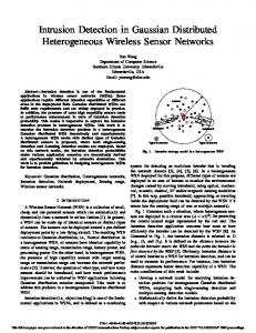
Fig. 1. Typical ball and ball-like objects in the frame. (Ball objects are marked by blue circles and nonball objects by red rectangles.) In (a) to (f), the upper halves are the original frames and lower halves are the corresponding processed frames, showing the ball and ball-like objects computed. Some typical appearance of the ball: (a) big ball; (b) medium and merged ball; (c) small ball; (d) flying ball; (e) flying ball; (f) merged ball. Typical appearance of ball-like objects: (a) glove; (b) soccer foots and other portions of players; (c) legs and other portions of players; (d) legs; (e) leg; (f) penalty mark and portions of players.
not hard to see that the features (e.g., shape, size, and color) of the ball are not very different from the features of the nonball objects in the same frame. In some cases, some nonball objects may look “more” like the ball than the ball itself. For example, when the ball is moving very fast or when it is partially occluded, the image of the ball is very far from the ideal perfect circle [as shown in Fig. 1(d) and (e)]. In the processed frames (obtained after removing other objects in the frame), it is clear that identifying the ball from the candidate ball objects is an extremely challenging task. This leads to one very fundamental difference between ball detection-and-tracking in BSV and other detection-and-tracking problems in the literature—there is no universal ball representation available that can be used to distinguish the ball from other ball-like objects within frame. In fact, in some frames, the image of the ball looks less like a ball than some other nonball objects! To overcome these challenges in ball detection and tracking, we propose a new trajectory-based strategy to develop an offline ball detection and tracking algorithm for BSV. In this strategy, there are
two phases, namely, the ball-candidate generation phase and the ball-trajectory selection and processing phase. In the first phase, we extend the search scope to identify a (small) number of ball candidates in each frame. In the second phase, we use trajectory information of these ball-candidate objects over a short sequence of frames to identify the ball trajectory (and prune off the nonball objects). Informally, the first key idea behind our strategy is that while it is very challenging to achieve high accuracy when locating the precise location of the ball, it is relatively easy to achieve very high accuracy in locating the ball among a set of ball-like candidates. We significantly reduce the rate of false negatives, but at the price of a temporarily higher rate of false positives. To eliminate the false positives, our second key idea is that it is much better to study the trajectory information of the ball since the ball is the “most active” object in the soccer video (as well as in most other sports video). For example, a ball-like object (say image of a ball on a T-shirt) is not likely to move significantly during the game. We believe that the strength of our new strategy
1166
IEEE TRANSACTIONS ON MULTIMEDIA, VOL. 8, NO. 6, DECEMBER 2006
comes mainly from careful control of false positives in the first phase and the trajectory-based processing in the second. Indeed, our experimental results show that the trajectory-based strategy can greatly enhance the accuracy of ball detection and tracking in BSV. The rest of this paper is organized as follows. In Section II, we describe the previous related work. Section III gives an overview of our trajectory-based ball detection-and-tracking algorithm. Section IV describes the methods for estimating the ball size while Section V presents the method for generating the set of ball-candidates for each frame. Section VI presents the method for generating the candidate trajectories. Section VII explains the methods to process the candidate trajectories to produce the ball trajectories and trajectory tracking. Experimental results are discussed in Section VIII. We conclude the paper in Section IX. II. RELATED WORK A. Related Work on Object Tracking There have been many object detection and tracking algorithms proposed over the last two decades. We can classify them into four broad categories: 1) feature-based; 2) model-based; 3) motion-based; and 4) data association algorithms. In feature-based algorithms, some features of object are used to discriminate targets from other objects within a frame. Some algorithms make use of a reference image of the background called the background frame. All objects in the “difference frame”—obtained by subtracting the background frame from the current frame—are targets [11]. In order to discriminate the target from other objects, features are used to characterize targets in the feature state space. Features such as parameterized shapes [7], [8], color distributions [21], shape and color together [19] are employed in the target representations. In [8], the features, together with manually-labeled targets are used to train a neural classifier, and then the trained neural classifier is used to differentiate the targets from other objects. Model-based algorithms, including anti-model algorithms, use not only features but also high-level semantic representation and domain knowledge to discriminate targets from other objects [12], [14]–[16], [34]. In both feature-based and model-based algorithms, the targets are detected one frame at a time and detection is performed using measures provided by features of the target. In these algorithms there are three main elements: target representation, feature extraction, and object discrimination. The principle of building a target representation is to make it feasible to discriminate the target from other objects and to make it easy to extract the features used in the representation. Thus, target representation can include appearance features, motion features, and models to solve the different problems. The representation has to be built up in the initialization, and then to be updated over frames. These algorithms make the implicit assumption that targets are “somehow different” from other objects within a frame. The intention of these methods is to decide whether a detected object is one of the targets in each frame. Motion-based algorithms rely on the methods for extracting and interpreting the motion consistency over frames (or time) to segment the moving object [2], [15]. Although the motion
consistency involves in some frames, motion-based algorithms still discriminate the target from other objects at the level of object and not at the level of trajectories. They do not have the ability to find the locations of the occluded targets. Data association algorithms are designed to solve the data association problem, which is a problem of finding the correct correspondence between the measurements for the objects and the known tracks [2], [6], [20], [22], [35]. There are four basic methods for data association problem: 1) nearest neighbor is a computationally efficient algorithm but is unreliable for tracking targets in a highly cluttered environment [6]; 2) track operation is a technique used in [6], [20], [22]. Current track operations include trajectory splitting originally proposed by Smith and Buechler [22], trajectory merging, and trajectory deleting [6], [20]. We describe the idea behind trajectory splitting (called track-splitting in [22]) since we also use it in our algorithm (Section VI). Suppose that a single target is tracked and two candidates (measurements) are found inside the validation area. Trajectory splitting forks the current trajectory into two, rather than arbitrarily assigning the closest candidate to the track. No assignment decision is made at this stage. Instead, decisions are postponed until additional candidates have been gathered to support or refute earlier assignments; 3) joint probabilistic data association, that enforces an “exclusion principle” to prevent two or more trackers from latching into the same target by making use of the target-measurement association probabilities jointly [19], [20]; and 4) multiple hypotheses tracking [6], [20], [22], which is based on a multiple scan method. These algorithms have high memory and computation requirements, which increase exponentially with problem size [6]. B. Related Work on Soccer Ball Detection and Tracking In contrast to general object detection and tracking, there have been many algorithms specially for locating the soccer ball. Success has been reported in [17] and [18] for the detection and tracking of the ball in the soccer video that are recorded by fixed camera, but these methods do not work well when they are applied to BSV. Gong et al. [9] designed the first algorithm to detect the ball in BSV as part of a bigger system. The algorithm uses only shape and color properties of the ball image to differentiate the ball from other objects and no details were given on experimental performance. Seo et al. [21] proposed an algorithm that does ball tracking in BSV. They use a Kalman filter-based template matching procedure to track the ball and use backprojection to predict possible occlusion. However, the algorithm requires manual input of the starting locations of the ball and the tracking result was not reported. D’Orazio et al. [7], [8] used a modified circle Hough transform (CHT) together with a neural network classifier to detect the ball for selected frames from real video (which is recorded by their own camera) rather than broadcast video. This method can obtain good results when the physical ball is a large ball in single color and the ball-deformation is not serious. However, the commonly used ball is small and is black and white, and there are many seriously deformed balls in BSV, as Fig. 1 shows. Moreover, the modified CHT and the neural network will fail to identify the ball when some nonball objects look like the ball
YU et al.: TRAJECTORY-BASED BALL DETECTION AND TRACKING IN BSV
1167
3 and 4. In this section, we first describe the preprocessing step performed on the broadcast sports video. We then give a highlevel overview of these main steps of the algorithm. The details of these steps are then given in the succeeding sections. A. Preprocessing of the Broadcast Soccer Video
Fig. 2. Block diagram of the trajectory-based ball detecting-and-tracking algorithm in broadcast soccer video.
more than the ball itself. Samples of typical nonball objects that are ball-like are shown in Fig. 1. C. Discussion on Past Algorithms for Soccer Ball Detection and Tracking Many of the previous algorithms work well with identifying balls that are reasonably well-defined or in specially prepared video settings [7]–[9], [17], [18]. However, for broadcast soccer video, the problem remains a challenging one—and these challenges were mentioned in the previous section. In particular, existing algorithms do not work well on occluded or merged balls. Some existing algorithms also use the idea of trajectory [25]—however, these are usually restricted to short trajectories over a small number of neighboring frames used for confirmation. We believe that our paper is the first that make use of the trajectory information over the entire video sequence in order to get more reliable ball trajectories and, from there, ball detection. In the process, we also make use of ideas in general object tracking, such as the trajectory splitting operation [22]. We also introduce some new operations such as trajectory trim and trajectory join to refine our trajectory-based method. We believe that the use of ball candidates and trajectory information is the key to our success with detecting even occluded or merged balls. III. OVERVIEW OF OUR TRAJECTORY-BASED ALGORITHM In this section, we elaborate on the key ideas behind our trajectory-based approach to ball detection-and-tracking in BSV. Fig. 2 shows the block diagram for our trajectory-based ball detection-and-tracking algorithm. There are four main steps: 1) Ball Size Estimation; 2) Ball-Candidate Detection; 3) Candidate Trajectory Generation; and 4) Trajectory Processing. The BallCandidate Generation Phase consists of Steps 1 and 2, while the Trajectory Selection and Processing Phase consists of Steps
Given any BSV, we first perform an offline statistical analysis to obtain the following information about the video that will be used as input to our algorithm: 1) the field color range; 2) the line color range—the color range of the various lines (center lines, center circle, out-of-bound lines, goal lines) on the field; 3) the team color ranges of both teams; and 4) color ranges for the goalkeepers and referees. We say that a frame contains the soccer field if and only if the dominant color of the frame falls in the field color range. Clearly, for ball detection and tracking, we are only interested in analyzing frames that contain the soccer field. Thus, we first partition the entire video into the , where each is a sesequences quence of contiguous frames that contain the field, and each is a sequence of contiguous frames that do not contain the field. We then perform ball detection-and-tracking on each of the sequences. Sequences that do not contain the field may be advertisement or frames that zoom into the spectators and these sequences are not analyzed. The physical size of the ball, the center circle, and the goalmouth are also given as inputs to our algorithm. B. The Ball-Candidate Generation Phase Recall that the key challenges for ball selection are: 1) there are many ball-like objects in a frame and 2) there is no universal ball representation that can be used to distinguish the ball from other ball-like objects in the frame. To partially resolve this challenge, our first key idea is to focus on generating a set of ball-candidates for each frame instead of attempting to identify the ball in each frame. We use the anti-model approach based on a set of sieves (anti-models).1 For each frame , we first identify the set of objects in the frame, denoted by . Then, we develop a set of sieves based on properties (such as ball size, color, shape) of the image of the ball in and use the sieves to sieve out nonball objects in . The remaining objects are the ball-candidates and they satisfy all the properties defined by the , the set of ball-candidates sieves. We denote this set by for frame . This process is illustrated in Fig. 1, where some of the ball-candidates are shown. A close inspection of these examples in Fig. 1 will find that it is very hard to identify the ball since they have all the from among the ball-candidates in properties of the ball. However, the probability that the ball is , is very high. among the ball-candidates, namely, The effectiveness of our anti-model approach is dependent on the accuracy of the sieves we define. The most important sieve is the one based on the ball size—it accounted for sieving out the majority of the objects. However, the ball size varies greatly in the different frames, and so we developed effective methods for estimating the size of the ball in each frame. We do this by first identifying a set of salient objects (such as the center circle in the field and the goalmouth) that are much more 1The notion of anti-models (sieves) is also used in other image processing applications, such as face identification [12].
1168
IEEE TRANSACTIONS ON MULTIMEDIA, VOL. 8, NO. 6, DECEMBER 2006
0
Fig. 3. Overview of the trajectory selection and processing process showing first, a CFP d plot for the BG sequence (frames 48957 to 49167), then the ball trajectory computed, and the final ball trajectory after post-processing. (For legibility, only even-numbered frames are drawn.) (a) Plot of the ball-candidates. Black dots, green rectangles, and red crosses stand for candidates of category 1, 2, 3. (b) Ball trajectories computed from the plot in (a). (c) Final ball trajectories after trajectory tracking and interpolation. (d) Illustration of the candidate trajectories. (Only some are plotted, otherwise the image becomes chaotic.)
reliable to identify and have known physical sizes. We then use this to compute the estimated ball size. For the sieves, we have used property thresholds that are a little loose in order to avoid false negatives. Therefore, while all the ball-candidates in satisfies the properties of the ball (defined by the sieves), they may still vary quite a bit. To distinguish among them, we classify according to their “likeness” to be the ball-candidates in the ideal ball. By storing only a small set of ball-candidates per frame, we can process all the ball-candidates in a long sequence of frames at the same time. When the ball-candidates are processed together, rich spatial and temporal information can be used in the next phase of the algorithm. C. The Ball-Trajectory Selection and Processing Phase At the end of the first phase, we have a set of ball-candidates, , for each frame . Recall that, within a frame , it is very
difficulty to identify the ball from among the ball-candidates in , as illustrated by the examples in Fig. 1. To resolve this difficulty, our second key idea is that it is much better to study the trajectory information of the ball since the ball is the “most active” object in the soccer video. Informally, our trajectory-based approach correlates information on the ball-candidates over a sequence of frames to help to separate the moving ball from the other ball-candidates. The first step (Step 3: Candidate Trajectory Generation) is the generation of a set of candidate trajectories for the video sequence. We first “visualize” the apparent motion2 of the all the ball-candidates by plotting the “locations” (or other features) of all the ball-candidates over time (as represented by the frame number). Fig. 3(a) shows an example of such a plot 2The apparent ball motion means the ball motion relative to the center of the frames, not the ball motion in the real world. However, the apparent ball motion is close to the ball motion in the real world when the camera is still.
YU et al.: TRAJECTORY-BASED BALL DETECTION AND TRACKING IN BSV
1169
which depicts the “location” of all the ball-candidates over time (the definition of plots is given in Section IV). In these plots, a moving object in the sequence (like the ball) will be depicted by a smooth trajectory over a (relatively) long period of time. However, nonball objects may exhibit short trajectories or no trajectory at all. We then compute a set of candidate trajectories based on these properties. The second step (Step 4: Trajectory Processing) is the selection of the ball trajectory and trajectory tracking. To identify good ball trajectories, we rank each candidate trajectory by a “confidence index” which is a heuristic measure that indicates the likelihood that it is a ball trajectory. The ranking information is then used in an iterative algorithm for selecting the set of ball trajectories. Fig. 3(b) shows the ball trajectory for the sequence in Fig. 3(a). Once the ball trajectories are computed, we do trajectory tracking where we “superimpose” the ball trajectory on the original frames and try to identify balls along the trajectory in the original frames that may have been missed in the earlier steps of the algorithm. We also try to extend the ball trajectory in both directions. Finally, we track the ball by interpolating the ball locations in short gaps between two adjacent trajectories. This interpolation allows us to track the ball when it is temporarily occluded or when the ball is momentarily out of the soccer field range. These trajectory post-processing steps make it possible for the trajectory to span over some frames in which the ball is actually occluded (say, by players) or out of the field portion if these are intermediate frames in the ball trajectory. IV. BALL SIZE ESTIMATION Accurate estimation of the ball size for each frame is important because the ball size varies greatly in the different frames. We do this with the help of a set of salient objects—fixed salient objects (the central circle and the goalmouth) with known physical sizes and moving salient objects (players) with estimated average physical sizes. These salient objects can be detected more easily and reliably, comparatively speaking. We first try to detect the center circle or the goalmouth. If these are not present in the frame, we detect the players in the field and compute their average size. For each frame , we first identify the size and location of these salient objects and use them to compute the ball size in . A. The Principle of Ball Size Estimation For a BSV, the camera can be approximately modeled by a pinhole camera and the imaging principle is illustrated in Fig. 4. Let and be the heights of the object and its image, respectively. Similarly, let and be the distances from the pinhole to the object and image, respectively. Then, we have (1) By computing the size of the image of a salient object with for the known physical size, we can calibrate the ratio for frame is given frame using (1). Then the ball size by , where is the known physical size of
Fig. 4. Pinhole camera model.
the ball. For each object, we define its normalized size to be the size of its image if it were located at the center of the frame. In general, we also need to account for the variation in image size between objects in various locations of the frame . Let be the height of the ball at the location in the frame ( and are the row and column locations of the ball in the frame, be the center of the frame and respectively). Let be the size of the ball image, if the ball were at . Then, by applying (1) twice, we have
(2) and are the distances between the pinhole where , reto the physical ball and the image of the ball at location and are the values of spectively. Also, and , respectively if the ball were at . Thus, we obtain the following size variation matrix, , for :
(3) is of dimensions , The size variation matrix and are the width and height of . We note that where (2) and (3) are approximate since we use the simplified camera model. Nevertheless, the approximation is accurate enough for estimation of the ball size for our purpose. has its own variation maStrictly speaking, each frame trix. But in BSV, there are largely three types of frames, namely, close-up view, far-view, and mid-view and we performed an offor each of fline calibration of the size variation matrix the three frame types. Within each of these three types, the variation in image sizes is small enough that the frame type can be determined by the approximate sizes of the salient objects detected. for an obWhile we can compute the value of ject of known physical size at location in the frame using . In our im(1), there is no way to determine plementation, an offline, manual procedure is used to select a number of high quality frames of the same frame type in which the ball is found in various positions of the frame. We can then use the relative sizes of the ball at various positions and linear . Using interpolation to obtain the size variation matrix this method, we obtain the size variation matrix for each frame type.
1170
Fig. 5. Ellipse detection process. (a) Input image. (b) Center line detected. (c) After frame transform and superimposition with the mirror image. (d) Ellipse detected, together with its bounding elliptic ring.
IEEE TRANSACTIONS ON MULTIMEDIA, VOL. 8, NO. 6, DECEMBER 2006
Fig. 6. Goalmouth detection process. (a) Input image. (b) Iimage segmented by line color. (c) Goalposts detected (as two short, parallel vertical lines). (d) Detected goalmouth.
B. Detection of Salient Objects Detection of the Center Circle: The most salient object in the BSV is the center circle which is intersected by the center line of the field. The center circle appears as a slightly oblique ellipse in the frame. There are many ellipse detection algorithms [10], [24], [27], [33] in the literature that can be used for detection of this ellipse. For our purpose, we need a fast algorithm that does not have to be extremely accurate. After experimenting with a few algorithms (including a fast robust ellipse Hough transform algorithm by the authors [27]), we settled on a much simpler and fast algorithm that exploits the special characteristics of the center circle in soccer videos. We give a brief description of the main steps of the algorithm, which are illustrated in Fig. 5. First, the algorithm detects the center line of the field illustrated in Fig. 5(b). We then transform the frame F so that the center line is vertical and located at the middle of the frame. The by-production is that the major axis of the ellipse is now horizontal. We superimpose the segmented image F with its mirror image with respect to the vertical center line. This helps to “fill in” pixels of the ellipse that are missing on one side of the ellipse and we get a more complete ellipse as illustrate in Fig. 5(c). Then, the vertical center line is removed, leaving only the ellipse. Finally, we project the points on the ellipse vertically to obtain the length of the major axis and horizontally to obtain the length of the minor axis. This gives the size of the ellipse in the image. The details of each step of this algorithm are presented in [27]. Goalmouth Detection: For the goalmouth, we have observed that: 1) the two goalposts are almost vertical; 2) the goalposts and goal bar are bold line segments; and 3) the goalposts are short line segments (compared to the center line and the sidelines). Again, we use these observations to design a simple and fast algorithm for goalmouth detection as illustrated in Fig. 6. The algorithm first find the two parallel vertical short line segand ) representing the goalposts. ments (denoted by lines
Fig. 7. Player detection process. (a) Input image. (b) Players detected, together with their bounding boxes.
This is similar to the procedure for finding the central line, except that these lines are shorter. Once these are identified, the algorithm for the existence of the goalbar (denoted by line ) connecting the upper endpoints of the two goalposts. The algorithm then detects the goal line (denoted by line ). The algorithm then refines these detected lines based on the composite information obtained. To further evaluate and confirm the existence of the goalmouth represented by the lines (namely, ), we use the following measure function defined by , where is the measure function for the line , whose value is the ratio of the number of line points to the number of all the points in the line area. Player Detection: We use a seed-growing procedure to find the set of objects (the connected components) that are in the field portion of the frame as shown in Fig. 7. Then, to remove the objects that are not players, we evaluate each object based on properties of the players. The properties we use are player color range (this range include the color range of players from both of teams, the goalkeepers, and the referees) and shape. Given be the number of pixels in , and an object , let be the number of pixels in that are in the player color range. denote the aspect ratio (ratio of height to width) Let
YU et al.: TRAJECTORY-BASED BALL DETECTION AND TRACKING IN BSV
1171
of the bounding box of the object . We define the following properties. . 1) Player color range property: 2) Player shape property: . and are constants. Objects that Here, the thresholds satisfy both properties are the detected players. Using the average size of the detected players, we can get the frame type. We compute their normalized sizes using the appropriate size vari. Lastly, the average player size of the frame ation matrix is the average of all its normalized sizes. C. Computation of the Ball Size We now describe the process of ball size estimation: Given the size and location of a salient object in a frame , we first determine the frame type of using the size of the object. Thus, we know the size variation matrix of F. Then, we use (2) to compute its normalized size of the salient object. Then we can . The ball size estimate the normalized ball size, for the detected ball at any location of the frame can be computed using (2). In addition, to account for errors during the segmentation and estimation processes, we use the size range defined by
(4) where and are small constants that are empirically determined. The choice of salient object depends on its availability and reliability. The center circle and goalmouth are very reliable. We use one of them whenever they can be detected. If they are both absent, or are not detected, then the average player size is used for size estimation. This is less reliable, but it suffices for building the ball-size sieve in Section V-B. V. BALL-CANDIDATE GENERATION In the ball-candidate generation phase, we process each frame in the sequence to obtain a set of ball-candidates . Given a frame , we first identify and “paint” the field portion of the frame using a simple seed growing procedure in which we continue to “absorb” neighboring pixels that are in or “very close” to the field color range. We eliminate the nonfield portion by classifying it as a nonball object3 and painting it with the standard field color. A. Computing the Set of Objects We now describe the procedure to compute the set of objects, , in the field portion of the frame . There are denoted by three steps in this procedure. O1: Identify, record and “remove” the set of salient objects (center circle, goalmouth and players). O2: Identify the set of objects in the remaining image. O3: Process the goalmouth area for possible ball objects. In step O1, we “remove” the detected salient objects by setting the corresponding pixel with the “standard” field color. 3Our algorithm detects only balls whose images are in the field portion of the frame and will miss those whose image lies outside of the field.
However, when removing circles and lines, special care must be exercised to ensure we do not “accidentally remove” the ball if it is merged with these objects. To this end, we remove only the pixels that belong to the center circle or the lines, as defined by their function representation we computed. Thus, if the ball is merged with the center circle, only the pixels that lie on the ellipse in the image are removed. The part of the ball that is “outside” the ellipse is retained. After step O1, the connected components that remain in the field portion are considered to be objects in frame . In step O2, we first extract this set of objects (connected components). In some frames, the ball may lie entirely inside another object (for example, the ball passing in front of a player). In these cases, the “embedded ball” may be pruned off together with the enclosing object. To handle these situations, we first segment that image obtained at the end of step O1 by the ball color range (coloring everything else the standard field color) and extract the objects that are formed. Special treatment must be accorded to the goalmouth area because when the ball is in the goalmouth area: 1) interesting events (such as goals) are likely to occur and 2) the area is very congested with players and so occlusion occurs more frequently. Step O3 handles this case and it proceeds as follows: Let be the current frame and be the previous frame. Assume that we have detected the goalmouth in and . We transinto to make the goalmouth in match the goalform mouth in exactly. Next, we obtain the frame difference, , obtained by “subtracting” the frame from frame , namely, , in which . The is in the pixel subtraction is defined as follows: if pixel is the field color, then the pixel ball color range and is kept, namely, ; otherwise, is painted with the standard field color. The salient clusters of are considered the objects. the points in nonfield color in Fig. 8 illustrates the procedure to produce objects in the goalmouth area. B. Defining the Sieves and Pruning the Nonball Objects To remove more nonball objects, we define a set of sieves based on various properties of the ball image. The most important of these is the ball-size sieve. The ball-size estimation is given by (4), as described in Section IV. be the number of pixels in , and Given an object , let be the number of pixels in that are in the ball color denote the aspect ratio (ratio of height to range. Let width) of the bounding box of the object . Let be the pixel location of the center of object c. In addition, let be the location of the penalty marker in the frame. These can be computed from the world location and known size of the penalty marker if the frame contains the goalmouth. The sieves are given as a set of sieving procedures. : Remove object whose size is not in Ball-Size Sieve the range defined by (4). : Remove all long lines and curves (since Line Sieve the ball cannot “deform” into a long line). : Remove an object if Ball-Color Sieve , where is a constant.
1172
IEEE TRANSACTIONS ON MULTIMEDIA, VOL. 8, NO. 6, DECEMBER 2006
Fig. 9. Candidate generation process. (a) Original frame. (b) Frame after removing nonfield and lines. (c) Frame after removing the objects by size. (d) Frame after removing objects by other sieves.
Fig. 8. Locating ball-like objects in the goalmouth area. (a) Previous frame. (b) Current frame. (c) Previous frame after goalmouth detection, segmentation, and transformation, denoted by F . (d) Current frame after goalmouth detection and segmentation, denoted by F . (e) Difference (F F ). (f) Salient cluster found.
0
Shape Sieve
: Remove an object if it does not satisfy , where is a constant . Ball-Center Sieve : Remove an object if the center pixel of does not fall in the ball color range. : Remove object if it is at locaPenalty Mark Sieve . tion After applying all the sieves to the objects in , the ones that remain (satisfy all the sieve properties) are the set of ball, of the frame . The sieved results candidates, denoted by of a frame are shown in Fig. 9. C. Classification of the Ball-Candidates We measure each ball-candidate against a number of properties of the “ideal” ball image and use these to classify the ball-candidates obtained. The properties used in our algorithm are size, circularity, and ball color range and separation. Given , let be its radius, be the a ball-candidate in be the number of pixels in number of pixels in , and that are in the ball color range. In addition, let is the estimated radius of the ball in the frame . We also define the notion of min-separation of a ball-candidate from other objects (including nonball objects) in the frame . Define the distance two objects and , denoted by , to be the distance between and at the points where they are nearest to each other. Then we define where
is the set of all objects in the frame . The min-separation property is defined to cater to nonball objects, such as socks and shoes of the players that may be segmented into separate ball-like objects. Some examples are illustrated in Fig. 1. These objects, which really are part of the players, are always close to the players. However, the ball will be away from the other objects in most of the frames. We define the following properties. . 1) Size property: 2) Min-separation property: . . 3) Color range property: . 4) Circularity property: A ball-candidate is said to be in Category 1 if it has all the properties defined above. Those that violate one of these properties are said to be in Category 2. Ball-candidates in the goalmouth are considered special and they are also classified as Category 2. All the other ball-candidates are classified in Category 3. Ball-candidates of category 3 are also kept since some of them may be partially occluded balls or merged ball. VI. CANDIDATE TRAJECTORY GENERATION At the end of the first phase, we have a set of ball-candidates, , for each frame . Recall that, within a frame , it is very difficult to identify the ball from among the ball-candidates in , as illustrated by the examples in Fig. 9. To resolve this difficulty, our second key idea is that it is much better to study the trajectory information of the ball since the ball is the “most active” object in the soccer video. Informally, our trajectory-based approach correlates information on the ball-candidates over a sequence of frames to help separate the moving ball from the other ball-candidates in the frame. , of candiThe first step is the generation of a set, date-trajectories for each video sequence . We start with some denote the frames in a video sedefinitions. Let quence and let be the set of ball-candidates for the
YU et al.: TRAJECTORY-BASED BALL DETECTION AND TRACKING IN BSV
frame . For each ball-candidate in located at pixel in the frame , we define its diagonal-distance location to be the distance between and the origin (0, 0). Diagonal-Time Plots: To “visualize” the apparent motion of the ball-candidates in the video sequence , we first plot some “feature” of the ball-candidates over time (as represented by the frame number). We call these plots candidate feature plots (CFPs). For example, if the “feature” selected is the diagonal-distance, then we call the resulting plot the CFP based for . In , each on diagonal-distance is represented by the point ). ball candidate in Fig. 3(a) shows an example of a over 211 frames, in which the ball-candidates are coded by shape and color—big black dots for Category 1, green rectangles for Category 2, and red crosses for Category 3. For legibility only, we displayed only the even-numbered frames. , the ball, the most active object, will be depicted In a by a smooth trajectory over a (relatively) long period of time. However, nonball objects may exhibit short trajectories or no trajectory at all. Therefore, to identify the ball trajectories, we first compute a set of candidate trajectories, and then choose the ball trajectories from among them. Location-Time Plots: For trajectory generation, we use the in which we plot the loCFP based on location , each cation of the ball-candidates over time. In the with location in the frame ball-candidate in is represented by the point . The is three-dimensional and has more discriminating power when locating is easier to visualize on paper. A trajectories, but the is also a trajectory in the , trajectory in the but the converse is not necessarily true. We use the to illustrate our ideas, but our algorithms use the for trajectory extraction. Informally, a trajectory is a sequence of points in the in which every two consecutive points are located near to each other. Visually, a trajectory traces a smooth curve in the . A trajectory T in the over the time interval is defined by a sequence of points, namely , where, for each (between and ), the point corresponds to a balland every two candidate in the frame with location , in the trajectory are located consecutive points, and close to each other, namely the distance and , where and are constant thresholds. Fig. 3(d) shows a sample of the candidate trajectories com. Note that these trajectories are plotted puted from the using the two-dimensional . Again, for legibility only, we did not show all the computed candidate trajectories as the resulting figure will be too chaotic. The Candidate Trajectory Generation Algorithm: To gen, severate the list of candidate trajectories from the eral algorithms can be used. We use a trajectory extension algorithm that extends a trajectory based on the apparent motion of . The algorithm uses a motion-based the objects in the Kalman filter is used for predicting the future location of the trajectory. The algorithm is simple, and is reused in other trajectory processing steps. Fig. 10 shows the flowchart of the trajectory
1173
N
Fig. 10. Flowchart of candidate trajectory generation. ( is a threshold.) of consecutive unsupported points and Z
is the number
extension algorithm. We first find a trajectory seed, which is a pair of ball-candidates from “consecutive” frames that are located close to each other. The algorithm starts with a trajectory and . It then iteratively extends the curseed, say at frames rent trajectory forward and backward in time, along the current direction of the trajectory. We describe only the forward extension—the backward extension is similar. A motion-based Kalman filter is used to model the apparent motion of this trajectory and to predict the location of the trajec. The algorithm then tries to tory in the next frame, at time verify the prediction, namely, locate a ball-candidate in frame that is at or near to the predicted location. If a unique ball-candidate verifies the prediction, the trajectory is extended and the algorithm continues the extension process. to time If the verification fails, then the Kalman filter continues to pre) dict the locations of the next few frames (up to frame until its prediction can be verified by a ball-candidate (say, for . Then, the trajectory is extended to frame . For the intermediate frames that are not verified, frame we use the predicted locations as points in the trajectory that are called unsupported points. (A trajectory point that has a corresponding ball-candidate is called a supported point.) The trajectory extension process terminates when the verificonsecutive frames (we use ). cation fails for The end point of the trajectory is the last supported point. The algorithm will then do a similar backward extension, after which , of candithe computed trajectory is added to the list, date-trajectories for . The algorithm then repeats the trajectory extension process with a new trajectory seed, as illustrated in Fig. 10. It is possible (although it is rare in practice) that during the verification step, there is a set of (nearby) ball-candidates, that verify the prediction—and so there is a fork in the current trajectory . This case is not handled in Fig. 10.
1174
IEEE TRANSACTIONS ON MULTIMEDIA, VOL. 8, NO. 6, DECEMBER 2006
However, we can extend it as follows: in this case, the algoto continue rithm chooses a ball-candidate from with the trajectory extension. For each ball-candidate bc, in , we store the partial trajectory , together with the current state of the Kalman filter in the seed pool for further processing later. We also change the initialization step so that if it selects a partially trajectory from the seed pool, then the Kalman filter will be restored to the saved state so that it can continue extension of the partial trajectory normally. Pruning Isolated Ball-Candidates: A close inspection of the in Fig. 3(a) shows that there are many isolated Category 3 ball-candidates (shown by the red crosses) that will never point (t, x, y) is called an be part of any trajectory. A isolated point if it corresponds to a Category 3 ball-candidate, and its nearest neighbor of Category 1 or 2 is greater than a . As a preprocessing step, we first remove all isothreshold lated points before calling trajectory generation algorithm. This speeds up the algorithm significantly. Patching Up Fragmented Trajectories: When a moving ball goes behind some players (and is temporarily occluded), the trajectory of the ball may be fragmented into several shorter, adjacent pieces. To patch up these types of fragmented trajectories, we use the following join operation. Consider two adjacent traover the time interval and over the time jectories, and . Let be the last ball-candidate in interval and let be the first ball-candidate in trajectory trajectory . We will join the trajectories and to get a new, combined trajectory if 1) the trajectories are close to each other, , and 2) the candidates and are close in will reterms of location and size. The combined trajectory and in . place both VII. TRAJECTORY PROCESSING , the Given the computed set of candidate trajectories next step is to select the set of ball in trajectories which we de. We start with some definitions. We say that note by two trajectories overlaps if their time intervals overlap, otherwise they are said to be disjoint. For any video sequence , the , consists of a set of disjoint ball trajectories of the ball, must be disjoint trajectories. Clearly, the trajectories in since there is at most one ball per frame. Therefore, the com, the “best” subset putational problem is to select from of ball trajectories. Confidence Index and Overlap Index: For each candidate tra, we define its confidence index, denoted by jectory in , that measures the confidence associated with being a ball-trajectory. The confidence index is a function of the type of be the number of canball-candidates in the trajectory. Let didates in and , , and be the number of candidates and in of category 1, 2, and 3, respectively. Let denote the fractions of the candidates in of category 1 and 2, respectively. Then, the confidence index of is defined by
(5)
(where ), and where the parameters , , , , are used to adjust the relative importance of the components. Clearly, we want ball trajectories to have a high confidence index. However, we cannot just choose the with the highest consubset of candidate trajectories in fidence index since they may not be mutually disjoint. In fact, in is selected to be a ball once a candidate trajectory trajectory, then all the other trajectories in that overlaps with must be removed from further consideration. However, there may be a trajectory with high confidence index but has a “very small” overlap with a ball trajectory . We define a trim operation that will remove (or “trim off”) the “small” overlapping portion in trajectory . We define the overlapping index, , between and , given by denoted by
(6) is the number of the frames in which and where overlaps. Given a ball trajectory , we apply the trim operais small tion to trajectories if its overlapping index (namely, ). A. Trajectory Selection We are now ready to present the Ball Trajectory Selection Algorithm. The algorithm takes as input a set of candidate trajectories, and produces as output, the set of ball-trajectories. The algorithm iteratively selects the candidate trajectory with the highest confidence index as a ball candidate . Then, the trajectories that overlap with are processed. Those with low overlap index are trimmed, while the others are discarded. The details of the algorithm are shown in Procedure 1. Procedure 1 Input: , the set of all candidate trajectories in the sequence; Initialize the set BT to be the empty set; while ( is not empty) do Let be trajectory in index;
with the highest confidence
; for (all trajectories
; in ) do
if
then
else
;
Output: BT, the set of ball trajectories for the sequence. Ball Detection Solution: After the set of ball trajectory for the sequence is determined, the ball detection solution is obtained as follows: Consider a frame at time . If the trajectory is a supported point in some trajectory , then we point in frame . If the trajectory say that the ball location is at is an unsupported point in some trajectory or if point there is no trajectory point for time , then we say that the ball
YU et al.: TRAJECTORY-BASED BALL DETECTION AND TRACKING IN BSV
cannot be detected in frame . This is the ball detection solution obtained after the trajectory selection step and we call this the trajectory selection solution (or TS solution) and we assess its effectiveness in our experimental evaluation. B. Ball Trajectory Tracking So far, the ball trajectory for a sequence is computed based on the information from only the ball-candidate sets in the sequence. While this is very effective and efficient, the process is not perfect. There are still unsupported points in the ball trajectories computed. We now describe a post-processing steps that attempts to partially remedy this. After the ball trajectory is computed, it is possible to reduce the number of unsupported points by searching for the “missing balls” in the original frames, in addition to the list of ball-candidates for the frames. Similarly, we also try to extend the trajectories using both the ball-candidates and the original frames. We call this process trajectory tracking. To do trajectory tracking, we use a modified version of the trajectory extension procedure (described earlier in Section VII). The modifications are: 1) instead of starting with trajectory seeds, we use only the ball for sequence and 2) when searching trajectory in for the ball for verification of the predicted locations, instead of using only ball-candidates, we use both the ball-candidates and the entire frame. In the modified verification step, we first search among the ball-candidates in the frame. If this is unsuccessful, we search for the ball in the original frame. To make this step more efficient, we make the following algorithmic refinements: we do not search the entire frame, instead we search only in a small region that encloses the predicted location of the ; and are the ball. This region should be current ball speed in the x and y directions, respectively. We do a local ball detection in this area using the ball size filter, the ball color range filter and the ball likeliness quality measure. With ball trajectory tracking, we are able to extend the trajectories and also decrease the number of unsupported points. This is the final ball detection solution obtained by our algorithm. C. Gap Interpolation Let and be two obtained ball trajectories. Let be and be the frame the frame number of the last frame in number of the first frame in . We compute the ball locations between and by using Kalman estimator from two directions if (we use , that means half a second). This interpolation procedure will give the ball locations when the ball is occluded temporarily or it is out of the camera view temporarily. VIII. EXPERIMENTAL RESULTS We have a C++ implementation of the trajectory-based ball detection and tracking algorithm. To test the performance of our algorithm, we used two videos recorded using a WinTV card connected to a TV antenna and stored in APL mpeg-1 format. Both videos were games from the FIFA 2002 World Cup—the , is the final match (Brazil versus Germany) and the first, , is the quarter-final game (Senegal versus Turkey). second, Preprocessing of the Video: For these videos, we first remove the nonfield sequences. We also remove all closed-up sequences
1175
since ball detection in closed-up frames is well-solved using existing methods (such as model-based algorithms [7]–[9]). The remaining video sequences are used for performance evaluation. In each sequence, a frame that contains the ball is called a ball frame, otherwise, it is called a no-ball frame. Ground Truth and Correctness: For the video sequence used, the ground truth is obtained by manual inspection. For each ball frame, we also record the location of the ball. An algorithm is said to correctly identify a frame if: 1) it detects the ball in the correct location when is a ball frame or 2) it detects that there is no ball when is a no-ball frame. An algorithm is said to give a false alarm if it detects a ball but in an incorrect location when is a ball frame or it detects a ball when is a no-ball frame. An algorithm is said to wrongly identify a frame if: 1) it does not detect a ball when is a ball frame or 2) it gives a false alarm. We use the following notations and conventions in presenting the results. Let #frm, #ball-frm (or #bf), #nb-frm be the numbers of frames in the sequence, ball frames, and nonball frames, respectively. For the performance of the algorithm, we let #correct denote the number of frames that the algorithm correctly identifies the ball and #false the number of false alarms. For performance of our trajectory-based ball detection and tracking algorithm, we give both the final results obtained, and the inter-solution, the result obtained after trajectory selecmediate tion. A. Baseline Evaluation Using the Video BG We use the BG video to perform baseline performance studies. For this purpose, we pre-selected nine sequences that represent a good mixture of characteristics: 1) far-view and middle-view; 2) ball and no-ball frames; and 3) short and mid-length sequences. There are a total of 2085 frames. The performance of our trajectory-based algorithm on these BG sequences is shown in Table I. (The start frame of the game in the video is frame 00001.) From Table I, we see that the trajectory-based algorithm performs extremely well on these pre-selected BG sequences, achieving an average accuracy of 98.4%, and 100% on six of them. We now consider the intermediate trajectory selection solution. For no-ball sequences (BG8, BG9), the accuracy is also 100%. For the other sequences, the results are very good, but there are more variations. For example, for sequence BG6 with a mixture of ball and no-ball frames, the accuracy is 70% for the trajectory selection solution. However, trajectory tracking was able to correct most of the error to push the final accuracy to 96.1%. Remarkably, the number of false alarms is negligible. We believe that part of the reason for this overall good performance may be that these pre-selected BG sequences are, relatively speaking, easier to solve. B. More Stringent Evaluation Using the Video ST Now we turn to more stringent tests of our algorithm using an entire video of the first half of the game ST, between Senegal and Turkey (FIFA2002). The field portion of the ST video is divided into 139 sequences, as shown in Table II. We discard the 15 replay sequences that are done with very different camera angles and are not suited for our algorithm.
1176
IEEE TRANSACTIONS ON MULTIMEDIA, VOL. 8, NO. 6, DECEMBER 2006
TABLE I PERFORMANCE OF OUR ALGORITHM ON THE NINE SELECTED BG SEQUENCES
TABLE II CLASSIFICATION OF THE SEQUENCES IN THE ST VIDEO
A sequence is called a no-ball sequence if the whole sequence does not contain the ball. On the 56 no-ball sequences (over 6385 frames), our algorithm achieves an accuracy of 100%. The remaining 68 sequences are classified into 14 short sequences, S01-S14 of lengths up to 300 frames, 40 medium sequences, M01-M40 of lengths from 301 to 1000 frames, and 14 long sequences, L01-L14 with more than 1000 frames. For a more stringent test, Table III shows the results for these 68 sequences, leaving out the 56 nonball sequences for which the algorithm achieves 100% accuracy. Table III shows that our algorithm achieves a final accuracy of about 81% on average for the ST video. It is slightly higher (87%) for the short sequences. The intermediate trajectory selection solution shows an accuracy of 72% on average. This result again shows the effectiveness of trajectory tracking in improving the accuracy—by an average of about 8.5% for the ST video. The rate of false alarm is very low—an average of only 1.1%, meaning that our detection results are very reliable. Furthermore, a more detailed analysis (not shown in the paper) reveals that, for each ball trajectory, the false alarms form a very small portion of the points in the trajectory. Thus, the ball trajectory results are also very reliable, which also help to explain the effectiveness of the trajectory tracking step. C. Comparison With the CHT Algorithm It is difficult to perform a head-to-head comparison with other algorithms since our algorithm performs both ball detection and tracking on broadcast soccer video while most algorithms in the literature do only ball detection or focus on other types of video input. As a reasonable comparison, we use our intermediate TS-solutions (without trajectory tracking) to compare against existing ball detection algorithms. We chose the algorithm by D’Orazio et al. [7], [8] that uses a CHT algorithm together with a neural network classifier for ball detection in soccer video. However, there are some differences in the actual setup. 1) Since we could not get the code of the algorithm, we implemented the CHT algorithm (but without the neural network clas-
sifier). 2) Their algorithm was designed to work well for videos recorded by their own camera, but we are using it on BSV, the ST sequences. To compensate for this, we assist the CHT algorithm by feeding in the list of ball-candidates we have computed in our algorithm. 3) We compare their results with our intermediate TS-solutions. Given these adjustments, Table IV shows the comparison of the CHT algorithm with our algorithm after trajectory selection for the 68 ST sequences. We note that the accuracy of CHT is about 46% compared to about 72% for our trajectory selection solution, and 81% for our final solution (from Table III). We observed that the CHT algorithm does not work on BSV well because many of the balls in BSV are not circular because: 1) they are partially occluded or 2) partially merged with other objects. To help account for this, we have separated the ball frames into: 1) N1 frames, in which the balls are neither occluded nor merged and 2) N2 frames, in which the ball is either occluded or merged. Overall, in the 68 ST sequences, and so if we remove the N2 frame from consideration (and assume that CHT fails in these frames), then the , accuracy of CHT goes up to about 90% which is quite close to the accuracy reported by [7] and [8]. D. Observations and Discussion The experimental results clearly demonstrate the effective of our trajectory-based ball-detection and tracking algorithm in BSV. The two prong approaches of using ball-candidates and then computing the ball trajectory to help identify the ball from the ball-candidates is very effective. For example, it achieves about 81% accuracy for the ST video. The algorithm is tolerant of minor errors made in some of the intermediate steps. As illustrated in Fig. 3(a), our ball-candidate generation procedure produces a sizable number of nonball candidates that look like the ball. Fortunately, the ball trajectory selection procedure is very effective in identifying the correct ball trajectories, as illustrated in Fig. 3(b). The ball trajectory also allows the trajectory tracking step to “recover” from errors made earlier in the algorithm as illustrated in Tables I and III. The comparison with the CHT algorithm supports our initial assertion that direct ball detection is extremely challenging in BSV since it is very hard to detect the balls in the frames where the ball is occluded or merged. In the ST sequences, about one third (31%) of the ball frames are frames with occluded or merged balls. Our experimental results show that CHT per-
YU et al.: TRAJECTORY-BASED BALL DETECTION AND TRACKING IN BSV
1177
TABLE III PERFORMANCE OF OUR ALGORITHM ON THE 68 SEQUENCES OF THE ST VIDEO
TABLE IV COMPARISON OF THE CHT ALGORITHM AND OUR TS-SOLUTION ON THE 68 SEQUENCES OF THE ST VIDEO
formed poorly on occluded and merged balls, while our algorithm was very successful in detecting occluded and merged ball with the use of trajectory selection and trajectory tracking.
IX. CONCLUSION AND FUTURE WORK Ball location in BSV is a challenging problem for a number of reasons and our own experimental results also support this claim. To solve this problem, we have presented a trajectorybased approach for offline ball detection-and-tracking in BSV. The experimental results show that our algorithm is very effective in ball detection—it does not only detect the ball, but also occluded balls and balls that are merged with other objects in the frame. There are two key ideas in this approach. The first is the use of a set of ball-candidates per frame (instead of direct ball selection). This greatly reduces the rate of misses and allows the inclusion of occluded balls and merged balls as ball-candidates. The second key idea is to the use of ball trajectories to assist in ball detection. In other words, to decide “whether a candidate trajectory is a ball trajectory” is more reliable than to decide “whether a ball-candidate is the ball”. Several other technical ideas were also presented in this paper that may be useful elsewhere: the use of anti-model approach is a fault-tolerant approach for ball-candidate generation. There are several avenues for future research work. One direction is to apply the trajectory-based approach to detect and track the balls in other sports video. We have successfully applied it to the tennis ball in broadcast tennis video [32]. We plan to apply this approach to other detection-and-tracking problems such as wildlife tracking and various surveillance tracking problems. Another direction is to use the approach and the trajectory results for other higher level tasks such as event detection in the soccer video. We have applied it for detection of events such as kicking, passing, shooting, and team ball possession—events which may be difficult to analyze based only on the low-level feature [30]. The algorithms in this paper can also be used to improve high-level semantic event detection such as goal.
REFERENCES [1] J. Assfalg, M. Bertini, C. Colombo, D. del Bimbo, and W. Nunziati, “Semantic annotation of soccer videos: automatic highlights detection,” Comput. Vis. Image Understand., vol. 92, pp. 285–305, 2003. [2] P. Bouthemy and E. Francois, “Motion segmentation and qualitative scene analysis from an image sequence,” Int. J. Comput. Vis., vol. 10, pp. 157–182, 1993. [3] J. E. Boyd and J. Meloche, “Evaluation of statistical and multiple-hypothesis tracking for video traffic surveillance,” Mach. Vis. Applicat., vol. 13, pp. 344–351, 2003. [4] R. G. Brown, Introduction to Random Signals and Applied Kalman Filtering: With MATLAB Exercises and Solutions, 3rd ed. New York: Wiley, 1997. [5] S. F. Chang, “The Holy Grail of content-based media analysis,” IEEE Multimedia, vol. 9, no. 2, pp. 6–10, Jun. 2002. [6] I. J. Cox, “A review of statistical data association techniques for motion correspondence,” Int. J. Comput. Vis., vol. 10, no. 1, pp. 53–66, 1993. [7] T. D’Orazio, N. Ancona, G. Cicirelli, and M. Nitti, “A ball detection algorithm for real soccer image sequences,” in Proc. ICPR, 2002, vol. 1, pp. 210–213. [8] T. D’Orazio, C. Guarangnella, M. Leo, and A. Distante, “A new algorithm for ball recognition using circle Hough transform and neural classifier,” Pattern Recognit., vol. 37, pp. 393–408, 2004. [9] Y. Gong, T. S. Lim, H. C. Chua, H. J. Zhang, and M. Sakauchi, “Automatic parsing of TV soccer programs,” in Proc. 2nd Int. Conf. Multimedia Computers and Systems, 1995, pp. 167–174. [10] J. Illingworth and J. Kittler, “A survey of the Hough transform,” Comput. Vis., Graph., Image Process., vol. 44, pp. 87–116, 1988. [11] K. P. Karmann, A. V. Brandt, and R. Gerl, “Moving object segmentation based on adaptive reference images,” in Proc. Conf. Eusipco, Barcelona, Spain, Sep. 1990, pp. 951–954. [12] D. K. Keren, M. Osadchy, and C. Gotsman, “Antifaces: A novel, fast method for image detection,” PRAMI, vol. 23, no. 7, pp. 747–761, 2001. [13] T. Kim, Y. Seo, and K. S. Hong, “Physics-based position analysis of a soccer ball from monocular image sequences,” in Proc. ICCV, 1998. [14] D. Koller, K. Danilidis, and H. Nagel, “Model-based object tracking in monocular image sequences of road traffic scenes,” Int. J. Comput. Vis., vol. 10, pp. 257–281, 1993. [15] G. Kuhne, S. Richter, and M. Berer, “Motion-based segmentation and contour-based classification of video objects,” in Proc. ACM Int. Conf. Multimedia, 2001, pp. 41–50. [16] D. Lowe, “Robust model based motion tracking through the integration of search and estimation,” J. Comput. Vis., vol. 8, pp. 113–122, 1992. [17] Y. Ohno, J. Miura, and Y. Shirai, “Tracking players and a ball in soccer games,” in Proc. Int. Conf. Multisensor Fusion and Integration for Intelligent Sys., Taipei, Taiwan, Aug. 1999. [18] ——, “Tracking players and estimation of the 3D position of a ball in soccer games,” in Proc. ICPR, 2000, vol. 1, pp. 145–148. [19] C. Rasmussen and G. Hager, “Joint probabilistic techniques for tracking multipart objects,” in Proc. CVPR, 1998, pp. 16–21. [20] ——, “Probabilistic data association methods for tracking complex visual objects,” IEEE Trans. Pattern Anal. Mach. Intell, vol. 23, no. 6, pp. 560–576, Jun. 2001.
1178
[21] Y. Seo, S. Choi, H. Kim, and K. Hong, “Where are the ball and players? Soccer game analysis with color based tracking and image mosaic,” in Proc. ICIAP, Sep. 17–19, 1997, pp. 196–203. [22] P. Simth and G. Buechler, “A branching algorithm for discriminating and tracking multiple objects,” IEEE Trans. Automat. Contr., vol. AC-20, pp. 101–104, 1975. [23] V. Tovinkere and R. J. Qian, “Detecting semantic events in soccer games: Towards a complete solution,” in Proc. ICME, 2001, pp. 1040–1043. [24] L. Xu and E. Oja, “Randomized Hough transform (RHT): Basic mechanisms, algorithms, and computational complexities,” CVGIP: Image Understanding, vol. 57, no. 2, pp. 131–154, 1993. [25] A. Yamada, Y. Shirai, and J. Miura, “Tracking players and a ball in video image sequence and estimating camera parameters for 3D interpretation of soccer games,” in Proc. ICPR, 2002, vol. 1, pp. 303–306. [26] X. Yu, “An Effective Trajectory-Based Algorithm for Ball Detection and Tracking With Application to the Analysis of Broadcast Sports Video,” Ph.D. dissertation, Dept. Comput. Sci., Nat. Univ. Singapore, Singapore, Aug. 2004. [27] X. Yu, H. W. Leong, C. Xu, and Q. Tian, “A robust and accumulatorfree ellipse Hough transform,” in Proc. ACM Conf. Multimedia, 2004, pp. 256–259. [28] X. Yu, Q. Tian, and K. W. Wan, “A novel ball detection framework for real soccer video,” in Proc. ICME, 2003, vol. II, pp. 265–268. [29] X. Yu, C. Xu, Q. Tian, and H. W. Leong, “A ball tracking framework for broadcast soccer video,” in Proc. ICME, 2003, vol. II, pp. 273–276. [30] X. Yu, C. Xu, H. W. Leong, Q. Tian, Q. Tang, and K. W. Wan, “Trajectory-based ball detection and tracking with applications to semantic analysis of broadcast soccer video,” in Proc. ACM Conf. Multimedia, 2003, pp. 11–20. [31] X. Yu, C. Xu, Q. Tian, X. Yan, K. W. Wan, and Z. Jiang, “Estimation of the ball size in broadcast soccer video,” in Proc. PCM 2003, 2003, pp. 929–934. [32] X. Yu, C. H. Sim, J. R. Wang, and L. F. Cheong, “A trajectory-based ball detection and tracking algorithm in broadcast tennis video,” in Proc. ICIP, 2004, pp. 1049–1052. [33] H. K. Yuen, J. Illingworth, and J. Kittler, “Detecting partially occluded ellipses using the Hough transform,” Image Vis. Comput., vol. 7, pp. 31–37, 1989. [34] T. Zhao and R. Nevatia, “Car detection in low resolution aerial image,” in Proc. ICCV, 2001, vol. 1, pp. 710–717. [35] Z. Zhang and O. D. Faugeras, “Three-dimensional motion computation and object segmentation in a long sequence of stereo frames,” Int. J. Comput. Vis., vol. 7, no. 3, pp. 211–241, 1992. Xinguo Yu (M’03) received the B.S. degree in mathematics from Wuhan University of Technology, Wuhan, China, the M.E. degree in computer engineering from Huazhong University of Science and Technology, Wuhan, China, the M.E. degree in computer applications from Nanyang Technological University,Singapore, and the Ph.D. degree from the National University of Singapore. He is currently a Research Scientist in the Institute for Infocomm Research in Singapore. His research interests include the video analysis, indexing and retrieval, video enhancement, computer vision, AGV routing, and approximation algorithms for NP-hard problems.
IEEE TRANSACTIONS ON MULTIMEDIA, VOL. 8, NO. 6, DECEMBER 2006
Hon Wai Leong (M’85) received the B.Sc. (Hons.) degree from the University of Malaya, Kuala Lumpur, Malaysia, and the Ph.D. degree from the University of Illinois at Urbana-Champaign. He is an Associate Professor in the Department of Computer Science, National University of Singapore. His research interests encompass the design of practical algorithms for optimization problems from many application areas, including computer-aided design of integrated circuits, transportation logistics, networking and multimedia systems, and computational biology. He is a member of ACM and ISCB and a Senior Member of the Singapore Computer Society.
Changsheng Xu (M’97–SM’99) received the Ph.D. degree in electric engineering from Tsinghua University, Beijing, China, in 1996. From 1996 to 1998, he was a Research Associate Professor with the National Lab of Pattern Recognition, Institute of Automation, Chinese Academy of Sciences. He joined the Institute for Infocomm Research (I2R), Singapore, in March 1998, where he is currently Head of the Media Analysis Lab. His research interests include multimedia content analysis, indexing and retrieval, digital watermarking, computer vision, and pattern recognition. He has published more than 100 papers in those areas.
Qi Tian (S’83–M’86–SM’90) received the B.S. and M.S. degrees from Tsinghua University, Beijing, China, and the Ph.D. degree from the University of South Carolina, Columbia, all in electrical and computer engineering. He was a Postdoctor Researcher at the University of California, San Diego, in 1985. He is currently a Principal Scientist at the Institute for Infocomm Research, Singapore. He is also an Adjunct Professor at Beijing University, Beijing, China. He joined the Institute of System Science, National University of Singapore, in 1992 as a Research Staff Member, and subsequently became the Program Director for the Media Engineering Program at the Kent Ridge Digital Labs, then the Laboratories for Information Technology, Singapore (2001–2002). His main research interests are image/video/audio analysis, multimedia content indexing and retrieval, computer vision, pattern recognition and machine learning. He has published over 110 papers in peer-reviewed international journals and conferences and has two U.S. patents issued, with four pending. Dr. Tian served as an Associate Editor for the IEEE TRANSACTION ON CIRCUITS AND SYSTEMS FOR VIDEO TECHNOLOGY (1997–2003) and as Chair and Member of numerous technical committees of international conferences, including the IEEE Pacific-Rim Conference on Multimedia (PCM), the IEEE International Conference on Multimedia and Expo (ICME), ACM-MM, and Multimedia Modeling (MMM).