Trajectory Optimization and Tracking of Hypersonic ...

中图分类号：论文编号：

硕士学位论文

基于高斯伪谱方法的高超声速飞行器轨迹优化及跟踪作者姓名

陶菲克

学科专业

飞行器设计

指导教师

周浩

培养院系

宇航学院

Trajectory Optimization and Tracking of Hypersonic Vehicle Using Pseudospectral Method

A Dissertation Submitted for the Degree of Master

Candidate: Tawfiqur Rahman Supervisor: Dr. Zhou Hao

School of Astronautics Beihang University, Beijing, China .

.

中图分类号：论文编号：

硕士学位论文

基于高斯伪谱方法的高超声速飞行器轨迹优化及跟踪

作者姓名指导教师姓名

陶菲克

申请学位级别

周浩

职

称

工学硕士

讲

师

学科专业飞行器设计

研究方向弹道优化设计

学习时间自 2009 年 5 月 1 日

起至 2011 年 6 月 11 日止

论文提交日期 20 年

论文答辩日期 20

学位授予单位

.

月

日

北京航空航天大学

学位授予日期

年

年

月

日

月

日

.

关于学位论文的独创性声明本人郑重声明：所呈交的论文是本人在指导教师指导下独立进行研究工作所取得的成果，论文中有关资料和数据是实事求是的。尽我所知，除文中已经加以标注和致谢外，本论文不包含其他人已经发表或撰写的研究成果，也不包含本人或他人为获得北京航空航天大学或其它教育机构的学位或学历证书而使用过的材料。与我一同工作的同志对研究所做的任何贡献均已在论文中作出了明确的说明。若有不实之处，本人愿意承担相关法律责任。

学位论文作者签名：

日期：

年

月

日

学位论文使用授权书本人完全同意北京航空航天大学有权使用本学位论文（包括但不限于其印刷版和电子版），使用方式包括但不限于：保留学位论文，按规定向国家有关部门（机构）送交学位论文，以学术交流为目的赠送和交换学位论文，允许学位论文被查阅、借阅和复印，将学位论文的全部或部分内容编入有关数据库进行检索，采用影印、缩印或其他复制手段保存学位论文。保密学位论文在解密后的使用授权同上。

.

学位论文作者签名：

日期：

年

月

日

指导教师签名：

日期：

年

月

日

.

Dedication To my beloved father who always encouraged me to do my master and PhD and contribute for the country. He passed away last month; could not live to see me making his dream mine and completing my first step.

.

BUAA Academic Dissertation for Masters Degree

摘要近年来，世界各国对高超声速飞行器的研究越来越多。根本原因是高超声速飞行器具有非常快的飞行速度。高超声速的飞行能力让人们期望着能将其作为武器（导弹）加以应用，从而可以在很短的时间内到达目标。不过，伴随高速性能而来的还有一系列复杂问题。在设计过程中，由于极高的速度带来了许多约束不得不考虑，例如，气动热、推进系统、飞行力学与控制等。这些约束的存在，大大减少了飞行器可行轨迹的存在空间。因此，研究满足约束条件的飞行器轨迹生成技术是很有必要的。本文研究了以冲压发动机作为主推进系统的某高超声速飞行器的轨迹生成问题，考虑了气动热、动压和过载等约束。优化算法采用了伪谱法。伪谱法是一种近来被广泛用于求解最优控制问题的方法，在航空航天领域获得了认可。因此，本文选用伪谱法最为基本的轨迹优化技术。文中分别应用了勒让德伪谱法和高斯伪谱法来优化高超声速飞行器的轨迹，并对两种方法的结果进行了对比分析。对飞行器的上升段、巡航段和下压段进行了优化。本文深入研究了应用伪谱法求解高超声速飞行器轨迹优化问题和不同的约束对飞行器轨迹的影响。本文假设地球为旋转球体，以三自由度点质量模型为研究对象。气动数据以及发动机参数等参考公开发表的相关文献。飞行器轨迹分为四段。首先，该飞行器从高度为 16000 米的高空飞行平台上发射，利用固体火箭发动机将飞行器加速，直到满足冲压发动机点火条件。冲压发动机工作以后，飞行器爬升，速度也不断增加。然后是高超声速巡航阶段，最后进行俯冲下压，燃料耗光。主要目标是在满足高超声速飞行约束下，使航程最大化。在采用伪谱方法之前，首先用直接打靶法对该问题进行了计算。为了实现不同的目标函数，利用 Simulink 模块构造了飞行器的动力学模型。分别用高斯伪谱法（GPM）和勒让德伪谱法（LPM）进行了轨迹优化。利用软件 GPOPS 实现了高斯伪谱法。勒让德伪谱方法是通过自己编程实现的。根据勒让德伪谱法基本原理，首先将最优控制问题离散为非线性规划（NLP）问题，然后利用序列二次规划（SQP）进行求解。 i


分别利用 SQP、GPM 和 LPM 进行了轨迹生成，并将得到的结果进行对比。结果证明了用于高超声速飞行器轨迹生成的数学模型和数值优化技术的可行性。同时，文中还提供了轨迹跟踪的一个可行解。本文利用 LPM 给出可行的制导策略。制导策略的研究有很好的发展前景。本文的研究为将来进一步研究更加鲁棒的轨迹跟踪技术和在线轨迹生成技术打下坚实的基础。

关键词：高超声速飞行器，轨迹优化，序列二次规划，高斯伪谱法，勒让德伪谱法，轨迹跟踪问题，线性反馈。

ii


Abstract Hypersonic vehicles are presently a seriously investigated concept. The reason for the ever increasing interest is the capability of hypersonic vehicles in moving at very high velocities. This capability provides ever growing prospect of this technology being used as weapons/missiles in reaching targets at very short time. However, with the innumerous prospects of hypersonic vehicle come complex issues of flight due to high velocity. Due to the range of velocities that a hypersonic vehicle travels at, there are constraints which arise from the complex issues of aero-thermodynamic interactions, propulsion system integration with flight dynamics and controllability. These constraints provide a much reduced space for a practically possible trajectory available for hypersonic vehicles. Therefore, trajectory generation of such vehicles has been investigated using different concept vehicle and methods. The present research deals with generation of feasible flight trajectory and tracking of this trajectory for a hypersonic vehicle considering scramjet propulsion system operation, aerothermodynamic constraint, dynamic pressure constraint and load factor constraint which need special consideration in case of hypersonic velocity flights. In optimizing or generating the trajectory, pseudospectral method was mainly used. Pseudospectral methods have recently been applied in numerous optimal control problems with very good prospect for application in the field of aeronautics. Therefore, this specific approach was chosen as the primary means for trajectory optimization of hypersonic vehicle. In pseudospectral methods, Legendre and Gauss pseudospectral methods were applied and compared. The trajectory was optimized for ascent, cruise and descent flight profiles. The research gives insight into the application of pseudospectral methods in hypersonic vehicle trajectory optimization and also effect of different constraints in trajectory of hypersonic vehicle. For generating the trajectory, the vehicle was modeled in 3 degrees of freedom considering a point mass model with rotating round earth assumption. The aerodynamic characteristics were determined using available data on hypersonic conceptual vehicle. The vehicle propulsion which is a scramjet system was modeled from relations and data available from open literature. The hypersonic vehicle profile that was chosen for optimization was a four phase profile. In the mission scenario, the vehicle is launched from an airborne platform at an altitude of

iii


16000 meters with a solid rocket motor which boosts the missile to appropriate velocity for scramjet ignition. On ignition of the scramjet propulsion, the vehicle ascents to a high altitude with increase in velocity. Then it cruises at the hypersonic velocity and finally goes on a descend profile upon exhaustion of fuel. The main objective is to maximize range throughout the profile under hypersonic constraints. Before application of pseudospectral method, the trajectory optimization problem was solved using Single shooting method. For this, a Simulink model of the missile dynamics was modeled which was then simulated to generate trajectory for different objective functions. Among pseudospectral methods, Gauss and Legendre pseudospectral method was applied for trajectory generation. Gauss pseudospectral method (GPM) was applied thorough General Pseudospectral and Optimal Control Software (GPOPS). And for Legendre pseudospectral method (LPM), code was written to discretize the optimal control problem to a Non Linear Programming (NLP) problem. This NLP problem was then solved using Sequential Quadratic Programming (SQP). With the generation of trajectory using SQP, GPM and LPM, a comparison was made of the trajectories attained. The results show the feasibility of the mathematical model and the applied optimization techniques in generating feasible hypersonic vehicle trajectories and the effects of the constraints in trajectory generation. It also gives a feasible tracking solution for the trajectory. Using this feasible solution a guidance scheme using LPM has been implemented. The guidance scheme has high prospects for further development. The research lays a strong foundation for further research into more robust trajectory tracking solution and onboard trajectory generation methods. Keyword:

Hypersonic vehicle, trajectory optimization, sequential quadratic programming,

gauss pseudospectral method, Legendre pseudospectral method, trajectory tracking problem, feedback linearization.

iv


Contents 摘

要

Abstract Contents ..................................................................................................................................... v List of Figures .......................................................................................................................... xi List of Tables ..........................................................................................................................xiii List of Abbreviations/Acronyms ............................................................................................ xv 1

Introduction ........................................................................................................................ 1 1.1

Background .............................................................................................................. 1

1.2

Hypersonic Vehicle/Missile Flight Profiles ............................................................. 1

1.3

Research Status ........................................................................................................ 4

1.4 2

1.3.1

Hypersonic vehicle trajectory optimization .................................................................... 4

1.3.2

Pseudospectral method in trajectory optimization .......................................................... 5

1.3.3

Pseudospectral guidance method for hypersonic vehicle ............................................... 5

Dissertation Structure .............................................................................................. 7

Vehicle Dynamics and Modeling....................................................................................... 9 2.1

Introduction.............................................................................................................. 9

2.2

Vehicle Model .......................................................................................................... 9

2.3

2.2.1

3 D Governing Equations ............................................................................................... 9

2.2.2

Aerodynamic Model ....................................................................................................... 9

2.2.3

Atmospheric Model ...................................................................................................... 13

2.2.4

Propulsion System Model ............................................................................................. 14

Flight phase wise modeling ................................................................................... 17 2.3.1

Ascent phase ................................................................................................................. 17 v


2.4 3

4

2.3.2

Cruise phase ..................................................................................................................17

2.3.3

Descend phase ...............................................................................................................17

Conclusion............................................................................................................. 18

Trajectory Optimization Methods ................................................................................. 19 3.1

Introduction ........................................................................................................... 19

3.2

Methods of Solving Trajectory Optimization Problems ....................................... 19 3.2.1

Indirect Method .............................................................................................................22

3.2.2

Direct method ................................................................................................................23

3.2.3

Differential Inclusion.....................................................................................................23

3.2.4

Shooting Method ...........................................................................................................23

3.2.5

Collocation Method .......................................................................................................24

3.2.6

Pseudospectral Method..................................................................................................25

3.3

Direct Single Shooting Method............................................................................. 25

3.4

Legendre Pseudospectral Method ......................................................................... 26

3.5

Gauss Pseudospectral Method............................................................................... 29

3.6

Comparative look at shooting and pseudospectral methods ................................. 31

3.7

Conclusion............................................................................................................. 32

Hypersonic Vehicle Trajectory Optimization................................................................ 33 4.1

Introduction ........................................................................................................... 33

4.2

Trajectory control variables .................................................................................. 34

4.3

4.2.1

Angle of attack ..............................................................................................................34

4.2.2

Bank Angle ....................................................................................................................34

4.2.3

Sideslip angle ................................................................................................................34

4.2.4

Equivalence Ratio..........................................................................................................35

System and operational constraints ....................................................................... 35 vi


5

4.3.2

Thermal Loads .............................................................................................................. 36

4.3.3

Load Factor ................................................................................................................... 36

4.3.4

Equilibrium Glide Condition ........................................................................................ 37

4.3.5

Propulsion System ........................................................................................................ 37

Flight Corridor Representation .............................................................................. 38

4.5

Conclusion ............................................................................................................. 39

Trajectory Generation ..................................................................................................... 41 5.1

Introduction............................................................................................................ 41

5.2

Vehicle trajectory ................................................................................................... 41

5.3

Trajectory Optimization using Single Shooting Method ....................................... 43

5.5

5.6

7

Dynamic Pressure ......................................................................................................... 35

4.4

5.4

6

4.3.1

5.3.1

Problem formulation for SSM ...................................................................................... 43

5.3.2

Simulink Model ............................................................................................................ 44

Trajectory Optimization using Gauss Pseudospectral Method .............................. 45 5.4.1

GPOPS .......................................................................................................................... 45

5.4.2

Problem formulation for GPM using GPOPS®............................................................. 46

5.4.3

Optimization process .................................................................................................... 48

Trajectory Optimization using Legendre Pseudospectral Method ........................ 48 5.5.1

LPM Code Setup .......................................................................................................... 49

5.5.2

Problem formulation for LPM ...................................................................................... 50

Conclusion ............................................................................................................. 53

Trajectory Tracking Using Pseudospectral Method ..................................................... 55 6.1

Introduction............................................................................................................ 55

6.2

Guidance Law using indirect Legendre Pseudospectral Method .......................... 55

6.3

Conclusion ............................................................................................................. 59

Legendre Pseudospectral Guidance System .................................................................. 61 vii


8

7.1

Introduction ........................................................................................................... 61

7.2

Pseudospectral Guidance Law Derivation ............................................................ 61

7.3

Conclusion............................................................................................................. 64

Results and Analysis ........................................................................................................ 65 8.1

Introduction ........................................................................................................... 65

8.2

Ascent phase Trajectory ........................................................................................ 65

8.3

8.4

8.2.1

Problem Specifications ..................................................................................................65

8.2.2

Optimized trajectory ......................................................................................................65

8.2.3

State parameters ............................................................................................................66

8.2.4

Control parameters ........................................................................................................68

8.2.5

Constraint parameters ....................................................................................................69

8.2.6

Comparison ...................................................................................................................70

Cruise Phase Trajectory......................................................................................... 70 8.3.1


8.3.2


8.3.3


8.3.4


8.3.5


8.3.6

Comparison ...................................................................................................................74

Descend Phase Trajectory ..................................................................................... 75 8.4.1


8.4.2


8.4.3


8.4.4


8.4.5


viii


8.4.6

8.5

Complete 3D Trajectory ........................................................................................ 79 8.5.1

9

Comparison................................................................................................................... 79

Comparison................................................................................................................... 83

8.6

Legendre Pseudospectral Guidance Result ............................................................ 84

8.7

Conclusion ............................................................................................................. 86

Conclusion and Future Work.......................................................................................... 87 9.1

Conclusion ............................................................................................................. 87

9.2

Future work............................................................................................................ 88

References................................................................................................................................ 89 Research Outcome .................................................................................................................. 95 Acknowledgement................................................................................................................... 97

ix


List of Figures Figure 1.1 Flight profile of X-43 vehicle ................................................................................... 2 Figure 1.2 Flight profile of X-51 vehicle ................................................................................... 3 Figure 2.1 Normal force coefficient ......................................................................................... 10 Figure 2.2 Axial force coefficients ........................................................................................... 11 Figure 2.3 Coefficient of Lift ................................................................................................... 12 Figure 2.4 Coefficient of Drag ................................................................................................. 12 Figure 2.5 Density variation with altitude ................................................................................ 13 Figure 2.6 Mass flow rate at 32.5 km altitude. ......................................................................... 14 Figure 2.7 Plot of specific impulse as function of mach number and altitude. ........................ 16 Figure 3.1 Classification of trajectory optimization methods .................................................. 20 Figure 3.2 Representation of single shooting method .............................................................. 25 Figure 3.3 Nodes for shooting and pseudospectral methods .................................................... 31 Figure 4.1 Hypothetical flight corridor of hypersonic vehicle ................................................. 38 Figure 4.2 Constraints and design space for hypersonic flight................................................. 39 Figure 5.1 Expected trajectory and mass, mach no and flight path angle variation. ................ 42 Figure 5.2 Illustration of problem formulation for SSM. ......................................................... 44 Figure 5.3 Illustration of GPM methodology. .......................................................................... 45 Figure 5.4 Illustration of Optimization Methodology in GPOPS............................................. 48 Figure 5.5 Illustration of LPM Methodology. .......................................................................... 49 Figure 5.6 Illustration of LPMOPT code structure. .................................................................. 50 Figure 7.1 Pseudospectral Guidance Model ............................................................................. 64 Figure 8.1 3D Trajectory in Ascent Phase ................................................................................ 66 Figure 8.2 Plot of State Paramters in Ascent phase. ................................................................. 68 Figure 8.3 Plot of control parameters in ascent phase .............................................................. 69 Figure 8.4 Trajectory and constraint altitude (ascent phase) .................................................... 69 Figure 8.5 Plot of State Parameters in Cruise Phase ................................................................ 73 Figure 8.6 Plot of control parameters in cruise phase .............................................................. 73 Figure 8.7 Plot of Trajectory and Constraint Altitude (cruise phase) ....................................... 74 Figure 8.8 3D Trajectory in Descend Phase ............................................................................. 75 Figure 8.9 Plot of state parameters in descend phase ............................................................... 77 Figure 8.10 Plot of control parameters in descend phase ......................................................... 78 xi


Figure 8.11 Trajectory and constraint altitude (descend phase) ............................................... 79 Figure 8.12 Complete trajectory using SSM ............................................................................ 80 Figure 8.13 Plot of state and control parameters for complete 3D trajectory (SSM) .............. 80 Figure 8.14 Complete trajectory using GPM ........................................................................... 81 Figure 8.15 Plot of state and control parameters for complete 3D trajectory (GPM).............. 81 Figure 8.16 Complete trajectory using LPM ........................................................................... 82 Figure 8.17 Plot of state and control parameters for complete 3D trajectory (LPM) .............. 82 Figure 8.18 Comparative plot of state and control parameters ................................................ 83 Figure 8.19 State parameters of reference trajectory and test cases ........................................ 85 Figure 8.20 Trajectory error in LPM Guidance ....................................................................... 86

xii


List of Tables Table 2.1 Normal and Axial Force Coefficient Data. ............................................................... 10 Table 2.2 Lift and Drag Coefficient Data. ................................................................................ 11 Table 2.3 Air Mass Flow Rate Data. ......................................................................................... 14 Table 2.4 Specific Impulse Data. .............................................................................................. 16 Table 3.1 Comparison of shooting and pseudospectral methods.............................................. 31 Table 5.1 SSM file execution details. ....................................................................................... 43 Table 8.1 Ascent Phase Boundary Condition ........................................................................... 65 Table 8.2 Comparison of optimized trajectory ......................................................................... 70 Table 8.3Cruise Phase Boundary Conditions ........................................................................... 70 Table 8.4 Comparison of optimized trajectory ......................................................................... 74 Table 8.5 Comparison of optimized trajectory ......................................................................... 79 Table 8.6 Comparison of complete trajectories ........................................................................ 83 Table 8.7 Test cases for guidance scheme validation ............................................................... 84

xiii


List of Abbreviations/Acronyms AAS

American Astronomical Society

AIAA

American Institute of Aeronautics and Astronautics

ATACMS

Army Tactical Missile System

BVP

Boundary Value Problem

CGL

Chebyshev Gauss Lobatto

DARPA

Defense Advanced Research Project Agency

DIDO

Direct Indirect Optimization

DRE

Differential Riccati Equation

GPM

Gauss Pseudospectral Method

GPOPS

General Pseudospectral Optimization Software

HLGL

Hermite Legendre Gauss Lobatto

HTV

Hypersonic Technology Vehicle

IEEE

Institute of Electrical and Electronic Engineering

SIAM

Society of Industrial and Applied Mathematics

LG

Legendre Gauss

LGL

Legendre Gauss Lobatto

LPM

Legendre Pseudospectral Method

LPMOPT

Legendre Pseudospectral Optimization Programme

LTV

Linear Time Varying

NASA

National Aeronautics and Space Administration

NLP

Non Linear Programming

PS

Pseudospectral Method

SCRAM

Supersonic Combustion Ramjet Missile

SQP

Sequential Quadratic Programming

SSM

Single Shooting Method

TPBVP

Two Point Boundary Value Problem

TPS

Thermal Protection System

xv


1 Introduction 1.1

Background Hypersonic flying machines powered by air-breathing scramjet engines are finally

coming into focus as the quick-response space launchers and super-swift far-ranging missiles of the future. Development of supersonic combustion propulsion for hypersonic vehicles is showing the positive results and solid promise that have proved elusive in the past. A key activity in the widening realm of hypersonic research is the X-51A program, in which the US Air Force, NASA, and DARPA (Defense Advanced Research Project Agency) have demonstrated a scramjet propelled vehicle that burns hydrocarbon fuel to propel a 14-ft airframe that looks like a missile. The X-51 made its maiden hypersonic flight for 200 seconds in May 2010. This demonstration provides future hopes for a long range, high speed and fast global strike weapon capable of reaching any target on the globe within minutes. This programme is a continuation of the efforts made in the development of X-43 hypersonic vehicle which also made hypersonic flight though for a very short period. There have been other programmes as well, like HyShot, SHMAC, and Brahmos etc. But so far X-51 has been the most encouraging demonstration. The missile flight profile for all the missile programmes so far are identical, in the sense that all have profiles in which they are launched from a carrier aircraft at high velocity in order to facilitate the high initial velocity required for the operation of scramjet engine. These flight profiles are available in many literatures. Flight profiles of different hypersonic missile/vehicle programmes available in these literatures are shown for future reference for the missile flight profile used in this thesis.

1.2

Hypersonic Vehicle/Missile Flight Profiles The earliest documented hypersonic missile project was the SCRAM (supersonic

combustion ramjet missile) programme, which was published in detail in 1995 by Billig. F.S. [1]. The programme ran from 1962 to 1978. The missile was launched by a solid rocket booster from the deck of a ship to a flight mach number of 3.5 to 4. After booster separation, the scramjet engines ignited and accelerated the system to a high flight mach number suitable for cruise. The missile was expected to cruise at sea level with Mach 6.5 and at 30,000 m at 1

Chapter 1 Introduction

Mach 8.5 with a payload of 56.7 to 65.8 kg to ranges in excess of 740 km at cruise altitudes of 30,000 m. It would be capable of intercepting low altitude targets by flying an optimum altitude and then dive to engage the target.

Figure 1.1 Flight profile of X-43 vehicle

The X-43A vehicle which paved the way for X-51, achieved maximum mach no of Mach 9.68 at an altitude of 112,000 feet on November 16, 2004 [2]. It was carried by NASA Dryden's B-52 aircraft to about 20,000 feet and released. The booster then accelerates the X43A research vehicle to the test conditions (Mach 7 or 10) at approximately 100,000 feet, where it separated from the booster and flew under its own power and preprogrammed control. The DARPA Falcon Hypersonic Technology Vehicle (HTV-2) programme is one of three designs underway to serve as the basis for the Conventional Prompt Global Strike weapon in order to hit a target anywhere in the world within an hour with a non-nuclear munition. The delta-wing-shaped carbon fiber aircraft was launched to the edge of space aboard a Minotaur4 rocket. The Lockheed Martin-built HTV-2 craft separated properly from the rocket’s faring and began a screaming glide over the Pacific Ocean intended to cover some 5,700 kilometers in less than half an hour [3]. The mission of X-51 followed a closely similar profile. It was carried by a B-52H and released at an approximate altitude of 45000 ft. after release, the X-51 was allowed to free fall for 4 seconds and then the ATACMS (Army Tactical Missile System) solid rocket ignites and 2


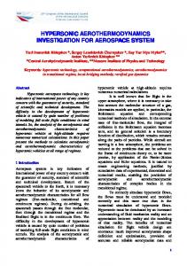
burns for 35 seconds, accelerating it to over Mach 4.5 at an altitude of 60,000 feet. During this boost phase, the scramjet inlet automatically start and aero heating begin to raise the temperature of the flow path walls as high speed air flows through the inlet and flow-through inter-stage. A small amount of JP-7 flow to fill the heat exchanger walls. Immediately prior to booster burnout, the cruiser separate from booster and inter-stage. After a minimal coast period, ethylene is injected and ignited in the flow path to complete the heating of the engine walls and JP-7 within. Once the fuel is heated to a minimum ignition temperature, the scramjet begins injecting hydrocarbon JP-7 fuel into the flow path. This transition phase lasts of several seconds until ethylene is fully expanded and the engine is operating solely on JP-7 fuel. With 265 lbs of JP-7 the period for scramjet operation is expected to be about 240 seconds. The planned optimized trajectory was to accelerate the vehicle to Mach 6. At about 240 seconds into flight, the unpowered phase starts by shutting down the engine. Then it starts gradually to dive to hit target. The flight profile is shown in Fig. 1.2 [4].

Figure 1.2 Flight profile of X-51 vehicle

Hypersonic missile concepts and projects utilize a delivery platform from which after release the hypersonic vehicle starts flight using a rocket motor and when adequate starting velocity is achieved for scramjet operation, the scramjet flight begins with aim to reach maximum speed and range. Finally on reaching target the missile makes dive on to the target.

3


This enables reaching any target on earth in less than an hour and thus gives prompt response capability.

1.3

Research Status Hypersonic vehicles are relatively new and therefore have only in last twenty years been

investigated in details. The research conducted in hypersonic vehicle trajectory generation and tracking guidance has been focused on designing of a flight trajectory that is feasible in terms of controllability and one that fulfills the constraints of hypersonic flight and can be tracked for the purpose of guidance. Such research has constraints in terms of non availability of adequate data on hypersonic vehicle aerodynamics, propulsion system integration and requirement of high level of accuracy due to hypersonic aerodynamics. This entails the need of accurate dynamic modeling of vehicle with integration of propulsion system and highly accurate scheme for computation. Computational scheme is in its own right a vast field and therefore warrants considerable proficiency and knowledge in selecting a suitable scheme for hypersonic vehicle trajectory generation and guidance. The present research trends direct the search for computational scheme towards shooting, collocation, differential inclusion and evolutionary algorithms. However, among all these available options, collocation methods especially pseudospectral methods have been of particular interest for hypersonic vehicle trajectory generation due to their fast convergence and accuracy. The detailed research status is further discussed in the following paragraphs. 1.3.1

Hypersonic vehicle trajectory optimization

Recently there have been many efforts in trajectory optimization of hypersonic vehicles for different phases of flight in different optimization methods. Yu Li and Nai-gang Cui has optimized multi phase, multi constraint trajectory under near real conditions for hypersonic missile in a boost-glide phase using sequential quadratic programming (SQP) [5]. Zhou Hao carried out a multi phase trajectory optimization for hypersonic vehicle for transition, glide and descent phase and did sensitivity analysis [6]. SUN Rui-sheng, XUE Xiao-zhong and SHEN Jian-ping optimized trajectory of hypersonic missile in extended range period by solving two point boundary value problem (from analytical optimal control solution method) by genetic algorithm [7]. A parallelized differential evolutionary algorithm was used to

4


optimize both steady-state and periodic trajectory of Waverider class missile for min-fuel, min-time-to-target and max-range by Ryan P. Starkey [8] [9]. Birendra V addressed the problem of trajectory optimization and guidance law synthesis for constant dynamic pressure ascent phase of typical air breathing launch vehicle in single stage to orbit (SSTO) mission for minimum fuel ascent using SQP [10]. Direct shooting method was used by Bing-nan Kang, Shuo Tang and Ryan P. Starkey in max-glide and fuel-optimal cruise trajectory optimization [11]. Jung-Woo Park, Min-Jea Tahk and Hong-Gye Sung investigated trajectory optimization of a supersonic air breathing missile using Legendre pseudospectral method [12] considering aerodynamic and propulsion system coupling for supersonic missile. These research works provide elaborate guidelines for flight dynamic modeling for hypersonic vehicle showing integration of aero-thermodynamic and aero- elastic characteristic in hypersonic velocity. 1.3.2

Pseudospectral method in trajectory optimization Pseudospectral methods have in recent years seen wide range application in trajectory

optimizations problems. Jeremy Rea applied Legendre pseudospectral method for launch vehicle trajectory optimization, [13] successfully to a three dimensional launch problem. The method was also demonstrated as a potential predictive guidance algorithm by finding both open and closed loop controls. Fariba Fahroo and I Michael Ross also presented a Chebyshev pseudospectral method for direct trajectory optimization [14]. They employ Nth degree Lagrange polynomial for state and control variables collocated at Chebyshev-Gauss-Lobatto (CGL) nodes to yield a non linear programming (NLP) problem. They conclude that pseudospectral methods produce more accurate results than traditional collocation methods. Timothy R. Jorris and Anil V. Rao demonstrated the performance of gauss pseudospectral method

through

multi-phase

implementation

programme

General

Pseudospectral

Optimization Software (GPOPS) against conventional optimization methods [15]. In line with the research trend, Jung-Woo Park and Min-Jea Tahk applied pseudospectral method in supersonic trajectory optimization [12]. A good number of literatures have been published on the scope of application of pseudospectral methods in trajectory optimization by I Michael Ross, Fariba Fahroo and Qi Gong [14] [16] [17] [18] [19] [20]. 1.3.3

Pseudospectral guidance method for hypersonic vehicle Guidance methods of hypersonic vehicle are more challenging than trajectory

generation problem due to the requirement of on-line calculation and the constraints of 5


hypersonic flight. In general guidance methods can be of predictor-corrector type or reference trajectory tracking type. Predictor-corrector guidance algorithms have long been used in mission analyses of various vehicles [21] [22]. Braun and Powell [23] have developed a predictor-corrector guidance algorithm. The algorithm computes bank angle and bank angle reversal logic to achieve the specified exit energy through NewtonRaphson iteration technique. Braun and Powell also provide an improved version of the predictor-corrector algorithm [24]. Similar research is also presented by J. Ashoke, K.Sivan, S.S. Amma [25], C.S. Gao, W.X. Jing, C.Y. Li [26] and Ping Lu [27]. Predictorcorrector algorithm propagates numerically along with the trajectory to predict the final condition and correctional steps to adjust the design parameters to null the error in meeting terminal condition. Predictor-corrector method is capable in guiding trajectory without any pre-stored data and gives greater flexibility in handling larger and unseen dispersion or disturbances. However, this method is not always practically implementable for highly constrained trajectories like hypersonic flight [28]. The first reason is that, computation becomes highly intensive, expensive and slow due to hypersonic flight constraints and therefore are at times incapable of real time calculation. The second problem is that convergence to optimal solution might require trial and error process which is not possible in real time environment. To cater these problems, trajectory tracking guidance comes as a prospective method for constrained trajectory guidance. In this method, feasible trajectory solutions are stored on on-board computer and tracked on-line for guidance. This enables the vehicle to fly on a trajectory that does not violate constraints and also can null errors arising from unforeseen disturbances if provided with an outer loop. Ping Lu presents a trajectory tracking method for regulating nonlinear dynamic system about linear time varying (LTV) system of reference trajectory [29]. G.A. Dukeman presents a similar guidance method using linear quadratic regulator (LQR) theory [30]. Similar profile following guidance schemes are researched by A.J. Roenneke, P.J. Cornwell, A. Marki [31][32] and K.D.Mease, D.T. Chen and P. Teufel [33]. All these methods involve online solution of Differential Riccati Equations (DRE) which is tedious and slow. This intensive solution therefore needs to be replaced by a faster and accurate method which can enable easy on-line application. Pseudospectral methods (PS) as discussed in the preceding section can be utilized here. In recent years, PS methods have shown considerable promise in solving such problems. Hui Yan, Fariba Fahroo and I. Michael Ross has presents state 6


feedback control laws for linear time-varying systems with quadratic cost criteria by an indirect Legendre pseudospectral method (LPM) which fast and accurate and able to compute control on-line [34]. This method obviated the need for solving the time-intensive backward integration of the matrix DRE or inverting ill-conditioned transition matrices. Kevin P. Bollino, I. Michael Ross and David D. Doman investigates the utility of a PS guidance algorithm for solving this problem and showed that it is capable of compensating for large uncertainties and disturbances [35].

1.4

Dissertation Structure This dissertation has been structured with the aim to reflect understanding of hypersonic

vehicle flight and its constraints, application of optimization methods in such trajectory which can then be used for guidance of the vehicle. The thesis can be seen as divided in three parts. First it discusses the issues related to hypersonic flight vehicle trajectory optimization. Then optimal control problem and pseudospectral methods in solving optimal control problems and optimal guidance is discussed. Through these the intension is to lay a basis for the onward elaborations about vehicle dynamics modeling and problem solving setup in the following three chapters. Then the results for the trajectory optimization are discussed. The complete work is presented in the following arrangement. Chapter 2 is where the presentation of the research starts with details on the modeling of vehicle and environment. Chapter 3 focuses on optimal control methods, their application in trajectory optimization problems. In this chapter, details on shooting method, Legendre pseudospectral method and gauss pseudospectral method has been presented. Chapter 4 discusses the issues of hypersonic vehicle trajectory in regard to control limitations and constraints. Chapter 5 then presents the modeling of the problem for the optimization methods and details on code structures. Chapter 6 presents the theoretical methodology of optimal guidance based on indirect pseudospectral method.

7


Chapter 7 presents implementation process for pseudospectral guidance system. Chapter 8 presents the results of hypersonic vehicle trajectory generation and guidance. Finally conclusion is drawn to the dissertation with light on onward research scopes enabled through this research.

8


2 Vehicle Dynamics and Modeling 2.1

Introduction Vehicle dynamics modeling and atmospheric modeling is the first step in aerospace

vehicle optimization. This chapter states the vehicle dynamic, aerodynamic and propulsion system and atmospheric model. As the research is on hypersonic vehicle, the constraints arising from hypersonic flight is also discussed here.

2.2

Vehicle Model The conceptual hypersonic vehicle model [36], has an empty weight of 2000 kg and

carries fuel of 1600 kg. The vehicle dynamics is modeled in 3D for trajectory optimization considering a point mass problem. The dynamic equations are stated in the following sections. 2.2.1

3 D Governing Equations The vehicle governing equations under the assumption of a flat earth is given as; 𝑟𝑟̇ = 𝑣𝑣𝑣𝑣𝑣𝑣𝑣𝑣𝑣𝑣

(2.1)

𝜙𝜙̇ = 𝑣𝑣𝑣𝑣𝑣𝑣𝑣𝑣𝑣𝑣𝑣𝑣𝑣𝑣𝑣𝑣𝑣𝑣 𝑟𝑟

(2.3)

𝑠𝑠𝑠𝑠𝑠𝑠𝑠𝑠 𝜃𝜃̇ = 𝑣𝑣 𝑐𝑐𝑐𝑐𝑐𝑐𝑐𝑐 𝑟𝑟 𝑐𝑐𝑐𝑐𝑐𝑐𝑐𝑐

𝑣𝑣̇ =

𝛾𝛾̇ =

𝑇𝑇𝑇𝑇𝑇𝑇𝑇𝑇𝑇𝑇 −𝐷𝐷 𝑚𝑚

(2.2)

− 𝑟𝑟𝜇𝜇2 𝑠𝑠𝑠𝑠𝑠𝑠𝑠𝑠 + 𝛺𝛺2 𝑟𝑟𝑟𝑟𝑟𝑟𝑟𝑟𝑟𝑟(𝑠𝑠𝑠𝑠𝑠𝑠𝑠𝑠𝑠𝑠𝑠𝑠𝑠𝑠𝑠𝑠 − 𝑐𝑐𝑐𝑐𝑐𝑐𝑐𝑐𝑐𝑐𝑐𝑐𝑐𝑐𝑐𝑐𝑐𝑐𝑐𝑐𝑐𝑐𝑐𝑐)

(𝑇𝑇𝑇𝑇𝑇𝑇𝑇𝑇𝑇𝑇 +𝐿𝐿)𝑐𝑐𝑐𝑐𝑐𝑐𝑐𝑐 𝑚𝑚𝑚𝑚

𝑣𝑣

+ 𝑐𝑐𝑐𝑐𝑐𝑐𝑐𝑐 � −

𝜓𝜓̇ = 𝐿𝐿𝐿𝐿𝐿𝐿𝐿𝐿𝐿𝐿 − 𝑣𝑣𝑣𝑣𝑣𝑣𝑣𝑣𝑣𝑣𝑣𝑣𝑣𝑣𝑣𝑣𝑣𝑣𝑣𝑣𝑣𝑣𝑣𝑣𝑣𝑣 𝑣𝑣𝑣𝑣𝑣𝑣𝑣𝑣𝑣𝑣 𝑟𝑟

𝑟𝑟

1

𝑣𝑣𝑟𝑟 2

� + 2𝛺𝛺𝛺𝛺𝛺𝛺𝛺𝛺𝛺𝛺𝛺𝛺𝛺𝛺𝛺𝛺𝛺𝛺 + Ω2 𝑣𝑣𝑣𝑣𝑣𝑣𝑣𝑣𝑣𝑣

−2Ω(𝑡𝑡𝑡𝑡𝑡𝑡𝑡𝑡𝑡𝑡𝑡𝑡𝑡𝑡𝑡𝑡𝑡𝑡𝑡𝑡𝑡𝑡𝑡𝑡 −𝑠𝑠𝑠𝑠𝑠𝑠𝑠𝑠 )+

𝛺𝛺 2 𝑟𝑟 𝑣𝑣

𝑐𝑐𝑐𝑐𝑐𝑐𝑐𝑐(𝑐𝑐𝑐𝑐𝑐𝑐𝑐𝑐𝑐𝑐𝑐𝑐𝑐𝑐𝑐𝑐 − 𝑠𝑠𝑠𝑠𝑠𝑠𝑠𝑠𝑠𝑠𝑠𝑠𝑠𝑠𝑠𝑠𝑠𝑠𝑠𝑠𝑠𝑠𝑠𝑠)

𝑠𝑠𝑠𝑠𝑠𝑠𝑠𝑠𝑠𝑠𝑠𝑠𝑠𝑠𝑠𝑠𝑠𝑠𝑠𝑠𝑠𝑠𝑠𝑠

(2.4) (2.5)

(2.6)

Here, r is radial distance from centre of earth, 𝜃𝜃 and 𝜙𝜙 are the longitude and latitude respectively, 𝑣𝑣 is velocity magnitude, 𝛾𝛾 is the flight path angle, and 𝜓𝜓 is the azimuth angle, m is vehicle mass, T is thrust.

2.2.2

Aerodynamic Model

The aerodynamic coefficients of the vehicle are given by normal force coefficient (cN) and axial force coefficient (cA) [36], which are functions of mach number (M) and angle of attack ( 𝛼𝛼 ). The lift and drag coefficients are calculated using Eq. 2.7 and 2.8. The 9

Chapter 2 Vehicle Dynamics and Modeling

aerodynamic coefficients are given in table2.1 and 2.2 and the plots of normal and axial force, lift and drag force coefficients are given in Fig. 2.1 to 2.4. 𝑐𝑐𝑙𝑙 = 𝑐𝑐𝑁𝑁 𝑐𝑐𝑐𝑐𝑐𝑐𝑐𝑐 − 𝑐𝑐𝐴𝐴 𝑠𝑠𝑠𝑠𝑠𝑠𝑠𝑠

(2.7)

𝑐𝑐𝑑𝑑 = 𝑐𝑐𝑁𝑁 𝑠𝑠𝑠𝑠𝑠𝑠𝑠𝑠 + 𝑐𝑐𝐴𝐴 𝑐𝑐𝑐𝑐𝑐𝑐𝑐𝑐

(2.8)

Table 2.1 Normal and Axial Force Coefficient Data.

°

𝐌𝐌/𝛂𝛂 3.5 4.0 5.0 6.0 6.5

𝟎𝟎 0.178 0.182 0.186 0.180 0.165

𝐌𝐌/𝛂𝛂 3.5 4.0 5.0 6.0 6.5

𝟎𝟎° 0.427 0.431 0.332 0.269 0.249

Normal Force Coefficients 𝟐𝟐° 𝟒𝟒° 0.681 1.183 0.646 1.112 0.589 1.002 0.540 0.915 0.504 0.865 Axial Force Coefficients 𝟐𝟐° 𝟒𝟒° 0.453 0.490 0.458 0.485 0.356 0.383 0.255 0.279 0.271 0.293

𝟔𝟔° 1.694 1.592 1.427 1.296 1.243

𝟖𝟖° 2.200 2.067 1.862 1.678 1.638

𝟔𝟔° 0.532 0.485 0.383 0.279 0.319

𝟖𝟖° 0.574 0.559 0.450 0.342 0.350

Plot of Coeffieicient of Normal Force

3 2.5

Coefficient of Normal Force

2 1.5 1 0.5 0 -0.5 -1 -1.5 -2 10 7

5 6.5 6

0

5.5

Angle of Attack (alpha)

5

-5

4.5 4 -10

3.5

Figure 2.1 Normal force coefficient

10

Mach No (M)

BUAA Academic Dissertation for Masters Degree Plot of Coeffieicient of Axial Force

0.3

Coefficient of Axial Force

0.25

0.2

0.15

0.1

0.05 10 7

5 6.5 6

0

5.5 5

-5

4.5 4 -10

Angle of Attack (alpha)

3.5 Mach No (M)

Figure 2.2 Axial force coefficients

Table 2.2 Lift and Drag Coefficient Data.

𝐌𝐌/𝛂𝛂 3.5 4.0 5.0 6.0 6.5

𝟎𝟎° 0.178 0.189 0.186 0.180 0.165

Lift Coefficients 𝟐𝟐° 𝟒𝟒° 0.665 1.146 0.629 1.075 0.576 0.973 0.530 0.893 0.494 0.842

𝟔𝟔° 1.628 1.533 1.379 1.259 1.203

𝟖𝟖° 2.009 1.969 1.782 1.614 1.574

𝐌𝐌/𝛂𝛂 3.5 4.0 5.0 6.0 6.5

𝟎𝟎 0.427 0.431 0.332 0.269 0.249

Drag Coefficients 𝟐𝟐° 𝟒𝟒° 0.477 0.571 0.480 0.561 0.376 0.452 0.274 0.342 0.288 0.352

𝟔𝟔° 0.706 0.649 0.530 0.413 0.447

𝟖𝟖° 0.874 0.841 0.705 0.572 0.575

°

11


Plot of Coeffieicient of Lift

3 2.5 2

Coefficient of Lift

1.5 1 0.5 0

-0.5 -1 -1.5 -2 10 7

5 6.5 6

0 Angle of Attack (alpha)

5.5 5

-5

4.5

Mach No (M)

4 -10

3.5

Figure 2.3 Coefficient of Lift Plot of Coeffieicient of Drag

0.8 0.7

Coefficient of Drag

0.6 0.5 0.4 0.3 0.2 0.1 0 10 7

5 6.5 6


5.5 5

-5

4.5 4 -10

3.5

Figure 2.4 Coefficient of Drag 12

Mach No (M)


From the available data on 𝑐𝑐𝑁𝑁 , 𝑐𝑐𝐴𝐴 and 𝑐𝑐𝑙𝑙 , 𝑐𝑐𝑑𝑑 the values of 𝑐𝑐𝑙𝑙 and 𝑐𝑐𝑑𝑑 can be expressed through the following polynomials as functions of 𝑀𝑀 and 𝛼𝛼 as in Eq. 2.9 and 2.10.

cl = (−0.0083M 3 + 0.1331M 2 − 0.7933M + 2.6476) × (0.0006α2 + 0.2002α + 0.1904)

(2.9)

cd = (−0.0292M 3 − 0.4339M 2 + 2.0014M − 2.3826) × (0.0015α3 − 0.0075α2 + 0.0677α + 0.7306) (2.10)

Lift and drag forces can then be calculated through Eq. 2.11 and 2.12. 1

𝐿𝐿 = 2 𝜌𝜌𝑣𝑣 2 𝑆𝑆𝑐𝑐𝑙𝑙

(2.11)

1

2.2.3

𝐷𝐷 = 2 𝜌𝜌𝑣𝑣 2 𝑆𝑆𝑐𝑐𝑑𝑑

Atmospheric Model

(2.12)

An exponential atmospheric density model as of Eq. 2.13 has been used for simulation. 𝜌𝜌 = 𝜌𝜌0 𝑒𝑒𝑒𝑒𝑒𝑒((𝑟𝑟 − 𝑅𝑅𝑒𝑒 )⁄𝐻𝐻 )

(2.13)

Here 𝜌𝜌0 equals to 1.225 kg/m3 and H is the scale height H = 7200m. The density variation

with altitude is shown in Figure. 2.5.

4

x 10

Plot of Air Density Variation with Altitude

4

3.5

3

Altitude (m)

2.5

2 Exponential Density Model

1.5 US Standard Atmosperic Model

1

0.5

0 0

0.2

0.4

0.6 0.8 Air Density (kg/m3)

1

Figure 2.5 Density variation with altitude

13

1.2

1.4


2.2.4

Propulsion System Model

The propulsion system modeled here is a hypersonic scramjet system. The modeling therefore includes expressions from air mass flow rate (𝑚𝑚̇𝑎𝑎𝑎𝑎𝑎𝑎 ), fuel flow rate (𝑚𝑚̇𝑓𝑓 ), specific impulse (𝐼𝐼𝑠𝑠𝑠𝑠 ) and thrust (𝑇𝑇).

The mass flow rate data [36] for the vehicle as function of 𝑀𝑀 and 𝛼𝛼 is given in table 2.3

for density corresponding to reference altitude ℎ∗ = 32500 m.

Table 2.3 Air Mass Flow Rate Data.

𝐌𝐌/𝛂𝛂 3.5 4.0 5.0 6.0 6.5

Air Mass Flow Rate 𝟐𝟐° 𝟒𝟒° 7.2387 8.2962 9.6937 10.6681 14.7104 16.6331 21.1998 24.7330 25.1683 29.6150

𝟎𝟎 6.9513 8.9355 12.7916 17.7370 21.5142 °

𝟔𝟔° 8.9447 11.6734 18.6106 26.8701 33.1770

𝟖𝟖° 9.6047 12.6860 20.3261 29.1919 35.2587

Plot of Mass Flow Rate of Air at 32.5 km

800

Mass Flow Rate of Air at 32.5 km

700 600 500 400 300 200 100 0 -100 -200 10 7

5 6.5 6


5.5 5

-5

4.5 4 -10

3.5

Mach No (M)

Figure 2.6 Mass flow rate at 32.5 km altitude. 14


From the available data, expression of 𝑚𝑚̇𝑎𝑎𝑎𝑎𝑎𝑎 ∗ with respect to 𝑀𝑀 and 𝛼𝛼 can be derived as

follows.

𝑚𝑚̇𝑎𝑎𝑎𝑎𝑎𝑎 ∗ = (−0.0083M 3 + 0.1331M 2 − 0.7933M + 2.6476) × (0.0006α2 + 0.2002α + 0.1904)

(2.14)

The mass flow rate of air at any altitude is expressed as; 𝑚𝑚̇𝑎𝑎𝑎𝑎𝑎𝑎 = 𝜌𝜌𝜌𝜌𝜌𝜌𝜌𝜌

(2.15)

Where, A is nozzle area, 𝑎𝑎 is sound velocity at the nozzle, 𝑀𝑀 is the Mach number at nozzle and 𝜌𝜌 is the density at given altitude. Therefore, the table data available [36] can be expressed through Eq. 2.16.

𝑚𝑚̇𝑎𝑎𝑎𝑎𝑎𝑎 ∗ = 𝜌𝜌∗ 𝑎𝑎∗ 𝑀𝑀∗ 𝐴𝐴

Therefore, 𝑚𝑚̇𝑎𝑎𝑎𝑎𝑎𝑎 for any given altitude can be found as in Eq. 2.17. 𝑚𝑚̇ 𝑎𝑎𝑎𝑎𝑎𝑎 ∗

𝑚𝑚̇𝑎𝑎𝑎𝑎𝑎𝑎 = �𝜌𝜌

∗ 𝑎𝑎 ∗ 𝑀𝑀∗

� × (𝜌𝜌𝜌𝜌𝜌𝜌)

(2.16)

(2.17)

From 𝑚𝑚̇𝑎𝑎𝑎𝑎𝑎𝑎 at given altitudes available, the fuel mass flow rate 𝑚𝑚̇𝑓𝑓 from Eq. 2.18 considering

constant stochiometric ratio as in Eq. 2.19.

𝑚𝑚̇𝑓𝑓 = 𝑚𝑚̇𝑎𝑎𝑎𝑎𝑎𝑎 𝜑𝜑𝑒𝑒𝑒𝑒𝑒𝑒𝑒𝑒 𝒻𝒻st

𝜑𝜑𝑒𝑒𝑒𝑒𝑒𝑒𝑒𝑒 = 𝒻𝒻 ⁄𝒻𝒻st , where 𝒻𝒻 = 𝑚𝑚̇𝑓𝑓 ⁄𝑚𝑚̇𝑎𝑎𝑎𝑎𝑎𝑎 and 𝒻𝒻st = 1/15

(2.18) (2.19)

Here 𝜑𝜑𝑒𝑒𝑒𝑒𝑒𝑒𝑒𝑒 is the equivalence ratio which regulated fuel flow rate in relation to air flow rate and is a control parameter for scramjet propulsion system [37] which in turn regulates thrust through Eq. 2.20. T = −𝐼𝐼𝑠𝑠𝑠𝑠 𝑚𝑚̇𝑓𝑓 𝑔𝑔

(2.20)

Here 𝐼𝐼𝑠𝑠𝑠𝑠 is calculated from available data which is given as functions of 𝑀𝑀 and ℎ in table 2.4.

The plot is given in Fig. 2.7.

15


Table 2.4 Specific Impulse Data.

𝐌𝐌/𝐡𝐡 3.0 4.0 5.0 6.0 7.0 8.0

12.5 km 1060 1060 969.9 855.2 724 596

Specific Impulse 20.0 km 25.0 km 1044.8 1024.8 1044.8 1024.8 952 931.2 837.6 816.8 712.8 697.6 592.8 580.8

15.0 km 1054.4 1054.4 964 848.8 719.2 594.4

30.0 km 1005.6 1005.6 909.6 799.2 687.2 569.6

35.0 km 976.8 976.8 879.2 775.2 668.8 542.4

40.0 km 943.2 943.2 847.2 749.6 644 499.2

Plot of Specific Impulse

1100

1000

Specific Impulse

900

800

700

600

500 8 7 10

6 Mach No

15 20

5

25 30

4 3

35

Altitude (km)

40

Figure 2.7 Plot of specific impulse as function of mach number and altitude.

16


2.3

Flight phase wise modeling The conceptual flight vehicle has an empty mass of 2000 kg. The modeling varies for

phases of flight. The differences among the phase wise modeling are mentioned in the following sections. 2.3.1

Ascent phase

At the time of launching from airborne platform, the vehicle carries a Lockheed Martin MGM-140A as solid rocket booster for initial boost. Therefore the initial mass is sum of empty mass, booster mass and fuel; after boost the booster is ejected and the vehicle starts to use the fuel mass with the initialization of scramjet propulsion. From this point the ascent phase begins. Here the vehicle consumes fuel which is consumed in producing thrust. This is controlled by equivalence ratio 𝜑𝜑𝑒𝑒𝑒𝑒𝑒𝑒𝑒𝑒 . Therefore, the vehicle

dynamic model for 7 state variables is composed of Eq. 2.1 to 2.6 and additional equation for rate of change of fuel mass 𝑚𝑚̇𝑓𝑓 Eq. 2.21.

𝑚𝑚̇𝑓𝑓 = − 𝐼𝐼

T

𝑠𝑠𝑠𝑠 𝑔𝑔

2.3.2

(2.21)

Cruise phase In cruise phase, the vehicle is still on propulsion and therefore the dynamic model

requires the same number of state and control variables. As in cruise there is no change in r, v and 𝛾𝛾, the dynamic equations for these parameters are as follows. 𝑟𝑟̇ = 0

(2.22)

𝛾𝛾̇ = 0

(2.24)

𝑣𝑣̇ = 0

(2.23)

Equations for the rest of the parameters remain as of those for ascent phase. 2.3.3

Descend phase

Descend phase of the vehicle is a zero propulsion phase and therefore modeling requires equations for only r, 𝜃𝜃, 𝜙𝜙, v, 𝛾𝛾, and 𝜓𝜓. And the control variables are only 𝛼𝛼 and 𝜎𝜎. 17


2.4

Conclusion The modeling of the problem vehicle has been described in this chapter. The modeling

includes vehicle dynamics in 3 DOF in a round rotating earth concept. The atmosphere has been modeled in an exponential way. The aerodynamics and propulsion system has been modeled from interpolation of available data on a conceptual hypersonic vehicle capable of an air launched missile type vehicle. With all these modeling scheme defined, the next step is to formulate the trajectory optimization problem for solution using SSM, GPM and LPM. This is detailed in the next chapter.

18


3 Trajectory Optimization Methods 3.1

Introduction Trajectory optimization is the process of designing a trajectory that minimizes or

maximizes some measure of performance within prescribed constraint boundaries. In the preliminary design of flight vehicles, selection of flight profile plays a very important role because the flight profile has to be designed in a way to yield the required performance. The flight profile of aerospace vehicle depends on the variation of the parameters that control the state of the vehicle. All the state, control, propulsion, structural, aerodynamic parameters are interrelated through flight-dynamic, aero-dynamic and other relations in ways that variation in a parameter effect the others. Therefore, the use of unplanned profile or control policies to evaluate competing configurations may inappropriately penalize the performance of one configuration over another. That means trajectory optimization can be defined as, the process to obtain both the state and control parameters which optimize the chosen performance index while satisfying existing constraints in the system. Although not exactly same, the objective of trajectory optimization is essentially the same as that of optimal control problem.

3.2

Methods of Solving Trajectory Optimization Problems Trajectory optimization problem which are essentially optimal control problem are

addressed in the analytical form in the optimal control literature by Bryson [38]. These optimal control problems can be solved in a number of ways numerically or analytically where the methods can be classified based on the differences in the steps of the process. The numerical approach can use either gradient or evolutionary algorithm. Gradient based method can be classified as direct or indirect methods. The scope of this research only covers direct method which can be further classified. A representation of the different available methods that are applied in optimal problem solution is shown in Fig. 3.1. The classification shows reclassifications of shooting and collocation methods both of which methods depend on discretization of parameters for optimization to transform optimal control problem to NLP problem.

19

Chapter 3 Trajectory Optimization Methods

Figure 3.1 Classification of trajectory optimization methods

In the most basic form of optimal control problem, given the equations of motion, boundary conditions, various types of constraints (equality, inequality; box constraints, general path constraints), and performance index or cost function, the solution is obtained through the calculus of variations [39]. First, a cost function is formed, augmented with Lagrange multipliers (or costates) associated with the constraints and state differential equations of the system. Defining a convenient Hamiltonian, the first variation of the cost function due to differential changes in the control inputs can be found. Then costate differential equations and boundary conditions are used to simplify the expression. The process of formulating a problem in terms of the original variables and Lagrange multipliers (or states and costates) is referred to as ‘dualization’ and this necessitates finding both the state and costate variables for optimization [39]. For the purpose of clarity, the process is further elaborated; Determine the control function 𝒖𝒖(𝑡𝑡) and the corresponding state trajectory 𝒙𝒙(𝑡𝑡), that

minimizes the Bolza cost function subject to state dynamics under the boundary constraints

20


and control limitations. An optimal control problem can be stated as finding the control vectors 𝒖𝒖(𝜏𝜏) and the resulting state vectors 𝒙𝒙(𝜏𝜏) which minimize the objective function Eq. 3.1, subject to dynamic constraints Eq. 3.2, boundary conditions Eq.3.3, 3.4 and path

constraints Eq. 3.5. 𝜏𝜏𝜏𝜏

ℑ�𝒙𝒙, 𝒖𝒖, 𝜏𝜏𝑓𝑓 � = ℳ�𝒙𝒙�𝜏𝜏𝑓𝑓 �, 𝜏𝜏𝑓𝑓 � + ∫𝜏𝜏0 ℒ[𝒙𝒙(𝜏𝜏), 𝒖𝒖(𝜏𝜏)]𝑑𝑑𝑑𝑑 ̇ = 𝑓𝑓[𝒙𝒙(𝜏𝜏), 𝒖𝒖(𝜏𝜏)], 𝒙𝒙(𝜏𝜏)

τ ∈ [𝜏𝜏0 , 𝜏𝜏𝑓𝑓 ]

𝜓𝜓0 [𝒙𝒙(𝜏𝜏0 ), 𝜏𝜏0 ] = 0

(3.1) (3.2) (3.3)

𝜓𝜓𝑓𝑓 �𝒙𝒙�𝜏𝜏𝑓𝑓 �, 𝜏𝜏𝑓𝑓 � = 0

(3.4)

𝛷𝛷[𝒖𝒖(𝜏𝜏)] ≤ 0

(3.5)

Here 𝑥𝑥 ∈ ℜ𝑛𝑛 , 𝑢𝑢 ∈ ℜ𝑚𝑚 and 𝑔𝑔 ∈ ℜ𝑟𝑟 . Then the augmented cost function is

𝒥𝒥̅ = ℳ�𝑥𝑥�𝜏𝜏𝑓𝑓 �, 𝜏𝜏𝑓𝑓 � + 𝜈𝜈0𝑇𝑇 𝜓𝜓0 [𝑥𝑥(𝜏𝜏0 ), 𝜏𝜏0 ] + 𝜈𝜈𝑓𝑓𝑇𝑇 𝜓𝜓𝑓𝑓 �𝑥𝑥�𝜏𝜏𝑓𝑓 �, 𝜏𝜏𝑓𝑓 � + 𝜏𝜏

𝑓𝑓 ∫𝜏𝜏 [ℒ(𝑥𝑥, 𝑢𝑢) + 𝜆𝜆𝑇𝑇 (𝜏𝜏){𝑓𝑓[𝑥𝑥(𝜏𝜏), 𝑢𝑢(𝜏𝜏)] − 𝑥𝑥̇ } + 𝜇𝜇 𝑇𝑇 (𝜏𝜏)𝑔𝑔(𝜏𝜏)𝑑𝑑𝑑𝑑 0

(3.6)

This, in term of augmented Hamiltonian form is

ℋ(𝑥𝑥, 𝜆𝜆, 𝑢𝑢) = 𝜆𝜆𝑇𝑇 𝑓𝑓 + ℒ + 𝜇𝜇 𝑇𝑇 𝑔𝑔

(3.7)

Where, the necessary optimality conditions are given by, 𝛿𝛿ℋ 𝛿𝛿𝛿𝛿

= 0,

𝜇𝜇 𝑇𝑇 𝑔𝑔 = 0,

𝜇𝜇 ≥ 0

Here, 𝜆𝜆(𝑡𝑡) is the Lagrange multiplier governed by the costate equation and transversality condition.

𝛿𝛿ℋ 𝜆𝜆̇ = − 𝛿𝛿𝛿𝛿 𝛿𝛿𝜓𝜓

(3.8) 𝑇𝑇

𝜆𝜆(𝜏𝜏0 ) = − �𝛿𝛿𝛿𝛿 (𝜏𝜏0 )� 𝜈𝜈 0

21

0

(3.9)

Chapter 3 Trajectory Optimization Methods 𝛿𝛿𝜓𝜓

𝛿𝛿ℳ

𝑇𝑇

(3.10)

𝛿𝛿𝜓𝜓 𝑓𝑓

(3.11)

𝜆𝜆�𝜏𝜏𝑓𝑓 � = 𝛿𝛿𝛿𝛿 (𝜏𝜏 ) + �𝛿𝛿𝛿𝛿 (𝜏𝜏𝑓𝑓 )� 𝜈𝜈 𝑓𝑓 𝑓𝑓

𝛿𝛿ℳ

ℋ�𝜏𝜏𝑓𝑓 � = − �𝛿𝛿𝜏𝜏 + 𝜈𝜈𝑓𝑓𝑇𝑇 𝑓𝑓

𝑓𝑓

𝛿𝛿𝜏𝜏 𝑓𝑓

�

As shown elaborately by I. Michael Ross and Fariba Fahroo [16] the transformation reformulates the problem in determining the state-costate-control function-triple, and the multipliers that satisfy a new set of differential algebraic equations that are the state, control and costate equations with a new set of boundary and necessary conditions. But these do not solve the problem easily rather this Legendre-Fenchel transformation [16] [40] makes it a two-point boundary value problem (BVP). Except in rare cases no analytical solution can be obtained for the BVP. Even linear BVPs do not have analytic solutions. That means that neither the original optimal control problem nor the dualized version involving costates can be solved analytically. Therefore, even for simple trajectory optimization problems, we need numerical methods. [16]. In order to use numerical method, the problem first has to be discretized. Discretization methods discretize the infinite dimensional problem into a finite dimension one. Discretization does not solve the problem; rather it gives a finite dimension problem which is a structured NLP problem that can be solved using numerical algorithms. Discretization can be applied to either a basic optimal control formulation or a primal dual space formulation (with costates). In the former case it is called a direct method and in the latter case it is an indirect method [16] [39]. 3.2.1

Indirect Method An indirect method discretize the system in its dualized form. That is, the states and

costates are both solved by solving the necessary conditions derived from the Pontryagin et al. minimum principle. While this gives greater accuracy than direct methods, some problems restrict the use. The problems are; firstly, analytical forms of the optimal control necessary conditions must be expressed, including the costate differential equations, the Hamiltonian, the optimality condition, and transversality conditions; it results in the same difficulty that is faced in analytical solution of optimal control problems. This also makes the problem size large due to discretization of the costates. Secondly, we need to guess certain aspects of the optimal control solution, such as the portions of the time domain containing constrained or 22


unconstrained control arcs, when using a gradient-based method. Thirdly, this involves costate variables whose physical meaning offers little help in determining reasonable initial guesses from which gradient search methods can converge. Therefore, the domain of convergence is generally very small [40]. 3.2.2

Direct method In order to avoid these problems, a direct discretization method can be used where the

system is discretized in its original form without the need to express the optimal control necessary conditions and costate equations. This does not require an analytical expression for the necessary conditions and typically does not require initial guesses for the adjoint variables [39]. Though direct methods are less accurate than indirect methods, the fact that they are easier to implement, have better convergence properties [14], and have reduced problem size makes them very attractive. Whether a direct or indirect method is chosen, the states must be integrated from some boundary condition or the equations of motion must be enforced through constraints. Direct methods can again be applied through shooting, collocation or differential inclusion. 3.2.3

Differential Inclusion

Differential inclusions strictly a direct method; enforces the equations of motion at each discrete node by applying inequality constraints on the state derivatives [41]. These inequality constraints are obtained by substituting the upper and lower bounds on the control vector into the equations of motion. When the inequality constraints are met, the states at one node are said to lie in the attainable set at that node given the state values at an adjacent node and the set of admissible controls. The advantage given by differential inclusions is that it effectively eliminates the explicit dependence on control values at each node [41]. However, it has been shown that, methods such as this can become numerically unstable and the formulation can be problem dependent [39]. 3.2.4

Shooting Method

Shooting method is another branch of direct numerical approach. This uses marching integration to calculate the state histories given the control histories of the system. The gradient-based algorithm then evaluates the objective function and constraint violations at

23


each discrete node. Shooting methods can be single or multiple types. Shooting methods are attractive because the equations of motion are enforced automatically by the marching integration. The direct shooting method is one of the most widely used methods and is especially effective for launch vehicle and orbit transfer applications. This method has the ability to describe the problem in terms of a relatively small number of optimization variables [39]. This effectively reduces the size of the problem by reducing the number of constraints. However, a direct shooting method requires very good initial guess to the actual but unknown solution. In case of a not so good initial guess, convergence becomes difficult. 3.2.5

Collocation Method Collocation methods enforce the equations of motion through quadrature rules or

interpolation [42]. An interpolating function is solved such that it passes through the state values and maintains the state derivatives at the nodes spanning one interval (or subinterval) of time. The interpolant is then evaluated at points between the nodes, called collocation points. At each collocation point, an equality constraint is formed, equating the interpolant derivative to the state derivative function, thus ensuring that the equations of motion hold (approximately) true across the entire interval of time [43]. The defining steps in the application of collocation method are; selection of the interpolating function and selection of nodes/collocation points within the time interval. The state and control parameters can then be approximated through the interpolating polynomials at these nodes. And the cost function and state equation can in turn be expressed in terms of these polynomial approximations. One of the simplest methods of collocation is the Hermite-Simpson method [43]. This method is so called because a third-order Hermite interpolating polynomial is used locally within many intervals, each solved at the endpoints of an interval and collocated at the midpoint. When arranged appropriately, the expression for the collocation constraint is the same as the Simpson integration rule. A generalization of the method to use the nth order Hermite interpolating polynomial, and choosing to take the nodes and collocation points from a set of Legendre-Gauss-Lobatto (LGL) points defined within the local time intervals, gives rise to the Hermite-Legendre-Gauss-Lobatto (HLGL) method [44] [45].

24


3.2.6

Pseudospectral Method Pseudospectral methods use global orthogonal Lagrange polynomials as the interpolant

while the nodes are selected as the roots of the derivative of the named polynomial, such as the Legendre-Gauss (LG), LGL or the Chebyshev-Gauss-Lobatto (CGL) points [14][17]. These pseudospectral methods use global orthogonal polynomials for approximation of control and state variables, instead of piece-wise-continuous polynomials. This approach is based on the idea given by Lanczos [46] that, a proper choice of trial functions and the distribution of collocation points is crucial to the accuracy of the approximating solution [47]. A merit of use of orthogonal polynomial is their close relationship to Gauss-type integration rules. This relationship can be used to derive simple rules for transformation of the optimal control problem to a system of algebraic equations [18]. Among the pseudospectral methods, Legendre and Gauss type are of main focus in this research.

3.3

Direct Single Shooting Method Direct single shooting method is based on the discretization of control variables. The time

domain is discretized into nodes where the control variables are discretized.

The state

variables are then regarded as dependent variables on the discretized time domain. Then numerical integration is used to obtain state values as functions of time and finite control parameters at the discretized nodes. This then gives a NLP problem which can be solved using NLP solvers like SNOPT® or fmincon in MATLAB®. The detail steps can be as shown below.

Figure 3.2 Representation of single shooting method

25


The optimal control problem mentioned earlier can be reformulated for single shooting method. The time domain [𝜏𝜏0 , 𝜏𝜏𝑓𝑓 ] is discretized as 𝜏𝜏𝑖𝑖 for 𝑖𝑖 = 0,1, ⋯ , 𝑁𝑁 in Eq. 3.12. 𝜏𝜏0 < 𝜏𝜏1 < 𝜏𝜏2 < ⋯ < 𝜏𝜏𝑛𝑛 = 𝜏𝜏𝑓𝑓

(3.12)

𝒖𝒖(𝜏𝜏) ≈ 𝒖𝒖(𝜏𝜏𝑖𝑖 , 𝑞𝑞), 𝑞𝑞 = (𝑞𝑞0 , 𝑞𝑞1 , 𝑞𝑞2 , ⋯ , 𝑞𝑞𝑁𝑁−1 )

(3.13)

The control parameters are now discretized and estimated at all the segments as Eq. 3.13.

Assuming that the discretization nodes for the state parameters are the same as of the control parameters, numerical integration can now be used to find the state variables as function of time and discretized control. 𝑁𝑁

𝒙𝒙(𝜏𝜏) ≈ 𝒙𝒙(𝜏𝜏𝑖𝑖 , 𝑞𝑞) = ∫𝑖𝑖=0 𝑓𝑓[𝒙𝒙(𝜏𝜏𝑖𝑖 , 𝑞𝑞), 𝒖𝒖(𝜏𝜏𝑖𝑖 , 𝑞𝑞)] , 𝑞𝑞 = (𝑞𝑞0 , 𝑞𝑞1 , 𝑞𝑞2 , ⋯ , 𝑞𝑞𝑁𝑁−1 )

(3.14)

Therefore, the optimal control problem can be written as a NLP problem as under where Eq. 3.15 is the objective function, Eq. 3.16 and 3.17 are the boundary conditions and Eq. 3.18 is the path constraint. 𝑁𝑁

ℑ�𝒙𝒙, 𝒖𝒖, 𝜏𝜏𝑓𝑓 � = ℳ�𝒙𝒙�𝜏𝜏𝑓𝑓 �, 𝜏𝜏𝑓𝑓 � + ∫𝑖𝑖=0 ℒ[𝒙𝒙(𝜏𝜏𝑖𝑖 , 𝑞𝑞), 𝒖𝒖(𝜏𝜏𝑖𝑖 , 𝑞𝑞)]𝑑𝑑𝜏𝜏𝑖𝑖 (3.15)

𝜓𝜓0 [𝒙𝒙(𝜏𝜏0 , 𝑞𝑞0 ), 𝜏𝜏0 ] = 0

(3.16)

𝛷𝛷[𝒖𝒖(𝜏𝜏𝑖𝑖 , 𝑞𝑞)] ≤ 0, 𝑖𝑖 = 0,1, ⋯ , 𝑁𝑁

(3.18)

𝜓𝜓𝑓𝑓 �𝒙𝒙�𝜏𝜏𝑓𝑓 , 𝑞𝑞𝑁𝑁−1 �, 𝜏𝜏𝑓𝑓 � = 0

3.4

(3.17)

Legendre Pseudospectral Method

Legendre Pseudospectral methods have been presented in papers by Elnagar, Kazemi and Razzaghi [47]. Application of this method in trajectory optimization has been demonstrated by I. Michael Ross and Fariba Fahroo [14] [18]. Here polynomial approximations of the state and control variables are considered where Lagrange polynomials are the trial functions and the unknown coefficients are the values of the state and control variables at the LGL points. By using the properties of the Lagrange polynomials, the state equations and the control constraints are transformed in to algebraic equations. The state differential constraints are 26


imposed by evaluating the functions at the LGL points and using a differentiation matrix that is obtained by taking the analytic derivative of the interpolating polynomials and evaluating them at the LGL points. The integral cost function can then be discretized by Gauss-Lobatto quadrature rule [47]. The optimal control problem can be formulated for LPM as follows. In LPM, the optimal control problem Eq. 3.1 to 3.5, is transformed into NLP problem through approximation of state (𝒙𝒙(𝜏𝜏)), control (𝒖𝒖(𝜏𝜏)) functions at LGL collocation points. As the above problem is formulated over the time domain [𝜏𝜏0 , 𝜏𝜏𝑓𝑓 ] whereas the LGL points lie

in the domain 𝑡𝑡𝑙𝑙 [-1, 1],𝑙𝑙 = 0, … , 𝑁𝑁, we require transformation of Eq. 3.1 to 3.5 to a new time

domain 𝑡𝑡𝑘𝑘 ∈ [𝑡𝑡𝑘𝑘 0 , 𝑡𝑡𝑘𝑘 𝑓𝑓 ] which has the similar spacing of LGL nodes and therefore represents 𝒙𝒙(𝜏𝜏) and 𝒖𝒖(𝜏𝜏) in correspondence to 𝑡𝑡𝑙𝑙 .

𝑡𝑡𝑘𝑘 = ��𝜏𝜏𝑓𝑓 − 𝜏𝜏0 �𝑡𝑡𝑙𝑙 + �𝜏𝜏𝑓𝑓 + 𝜏𝜏0 ��/2

(3.19)

Therefore the optimal control problem Eq. 3.1 to 3.5 is now represented as 𝜏𝜏 𝑓𝑓 −𝜏𝜏 0

ℑ�𝒙𝒙, 𝒖𝒖, 𝜏𝜏𝑓𝑓 � = ℳ �𝒙𝒙 �𝑡𝑡𝑙𝑙 𝑓𝑓 � , 𝜏𝜏𝑓𝑓 � + �

2

𝒙𝒙(𝑡𝑡̇ 𝑙𝑙 ) = 𝑓𝑓[𝒙𝒙(𝑡𝑡𝑙𝑙 ), 𝒖𝒖(𝑡𝑡𝑙𝑙 )],

𝑡𝑡

� ∫𝑡𝑡 𝑙𝑙 𝑓𝑓 ℒ[𝒙𝒙(𝑡𝑡𝑙𝑙 ), 𝒖𝒖(𝑡𝑡𝑙𝑙 )]𝑑𝑑𝑡𝑡𝑙𝑙 𝑙𝑙 0

𝜓𝜓0 �𝒙𝒙�𝑡𝑡𝑙𝑙 0 �, 𝑡𝑡𝑙𝑙 0 � = 0

𝜓𝜓𝑓𝑓 �𝒙𝒙 �𝑡𝑡𝑙𝑙 𝑓𝑓 � , 𝑡𝑡𝑙𝑙 𝑓𝑓 � = 0 𝛷𝛷[𝒖𝒖(𝑡𝑡𝑙𝑙 )] ≤ 0

𝑡𝑡𝑙𝑙 ∈ [−1, 1]

(3.20) (3.21) (3.22) (3.23) (3.24)

Now if LN (𝑡𝑡𝑘𝑘 ) are the Legendre polynomials of degree N on the LGL domain [-1, 1] and 𝑡𝑡𝑙𝑙

are the zeros of LṄ (t) then global polynomial expression of 𝒙𝒙(𝑡𝑡𝑘𝑘 ) and 𝒖𝒖(𝑡𝑡𝑘𝑘 ) can be written

as;

𝑁𝑁

𝒙𝒙(𝑡𝑡𝑘𝑘 ) ≈ 𝒙𝒙𝑁𝑁 (𝑡𝑡𝑘𝑘 ) = �𝑙𝑙=0 𝒙𝒙(𝑡𝑡𝑙𝑙 )𝜑𝜑𝑙𝑙 (𝑡𝑡𝑘𝑘 ) 𝑁𝑁

𝒖𝒖(𝑡𝑡𝑘𝑘 ) ≈ 𝒖𝒖𝑁𝑁 (𝑡𝑡𝑘𝑘 ) = �𝑙𝑙=0 𝒖𝒖(𝑡𝑡𝑙𝑙 )𝜑𝜑𝑙𝑙 (𝑡𝑡𝑘𝑘 )

Where 𝜑𝜑𝑙𝑙 (𝑡𝑡𝑘𝑘 ) are the Lagrange polynomials of order N. 1

𝜑𝜑𝑙𝑙 (𝑡𝑡𝑘𝑘 ) = 𝑁𝑁(𝑁𝑁+1)𝐿𝐿

(𝑡𝑡 𝑘𝑘 2 −1)𝐿𝐿̇ 𝑁𝑁 (𝑡𝑡 𝑘𝑘 ) 𝑡𝑡 𝑘𝑘 −𝑡𝑡 𝑙𝑙 𝑁𝑁 (𝑡𝑡 𝑙𝑙 )

27

(3.25) (3.26)

(3.27)


In order to carry out the second step of the collocation method, from the imposed condition that the above polynomial approximation of state and control variables, satisfy the system differential equations exactly at the LGL collocation points, the derivatives of state can be written as Eq. 3.28 [47]. 𝑁𝑁

𝑥𝑥̇ 𝑁𝑁 (𝑡𝑡𝑘𝑘 ) = �𝑙𝑙=0 𝐷𝐷𝐿𝐿𝐿𝐿𝐿𝐿 𝑘𝑘𝑘𝑘 𝑥𝑥(𝑡𝑡𝑙𝑙 )

(3.28)

Where 𝐷𝐷𝐿𝐿𝐿𝐿𝐿𝐿 𝑘𝑘𝑘𝑘 are the entries of the (N + 1) × (N + 1) differentiation matrix 𝑫𝑫𝑳𝑳𝑳𝑳𝑳𝑳 [17] [47]. 𝐃𝐃𝐋𝐋𝐋𝐋𝐋𝐋 ∶= [𝐷𝐷𝐿𝐿𝐿𝐿𝐿𝐿 𝑘𝑘𝑘𝑘 ] ∶=

L N (𝑡𝑡 𝑘𝑘 )

1

⎧ L N (𝑡𝑡 𝑙𝑙 ) .(𝑡𝑡 𝑘𝑘 −𝑡𝑡 𝑙𝑙 ) ⎪−N (N +1) ⎨ ⎪ ⎩

4 N (N +1) 4

0

k≠l

k=l=0

(3.29)

k=l=N otherwise

Next the integral in Eq. 3.20 is discretized substituting Eq. 3.25 and 3.26 and using the GaussLobatto integration rule; 𝑡𝑡 𝑙𝑙 𝑓𝑓 𝜏𝜏𝑓𝑓 − 𝜏𝜏0 � � ℒ[𝒙𝒙(𝑡𝑡𝑙𝑙 ), 𝒖𝒖(𝑡𝑡𝑙𝑙 )]𝑑𝑑𝑡𝑡𝑙𝑙 2 𝑡𝑡 𝑙𝑙

ℑ�𝒙𝒙, 𝒖𝒖, 𝜏𝜏𝑓𝑓 � = ℳ �𝒙𝒙 �𝑡𝑡𝑙𝑙 𝑓𝑓 � , 𝜏𝜏𝑓𝑓 � + �

= ℳ �𝒙𝒙 �𝑡𝑡𝑙𝑙 𝑓𝑓 � , 𝜏𝜏𝑓𝑓 � + �

𝜏𝜏 𝑓𝑓 −𝜏𝜏 0


= ℳ�𝒙𝒙𝑁𝑁 (𝑡𝑡𝑘𝑘 )� + �

2

2

0

𝑁𝑁 � ∑𝑁𝑁 𝑙𝑙=0 ℒ[∑𝑙𝑙=0 𝒙𝒙(𝑡𝑡𝑙𝑙 )𝜑𝜑𝑙𝑙 (𝑡𝑡𝑘𝑘 ), 𝒖𝒖(𝑡𝑡𝑙𝑙 )𝜑𝜑𝑙𝑙 (𝑡𝑡𝑘𝑘 )] 𝜔𝜔𝑘𝑘 𝑁𝑁

� �𝑙𝑙=0 ℒ�𝒙𝒙𝑁𝑁 (𝑡𝑡𝑘𝑘 ), 𝒖𝒖𝑁𝑁 (𝑡𝑡𝑘𝑘 )� 𝜔𝜔𝐿𝐿𝐿𝐿𝐿𝐿 𝑘𝑘

Here 𝜔𝜔𝐿𝐿𝐿𝐿𝐿𝐿 𝑘𝑘 are the weights given by Eq. 3.31. 2

𝜔𝜔𝐿𝐿𝐿𝐿𝐿𝐿 𝑘𝑘 = N(N+1) . [ L

1

2 N (𝑡𝑡 𝑘𝑘 )]

,

k = 0,1, ⋯ , N

(3.30)

(3.31)

The state equations and initial and terminal state conditions are discretized by substituting Eq. 3.25 to 3.29 in Eq. 3.21 and collocating at the LGL nodes 𝑡𝑡𝑘𝑘 . Using the notations for a and b, the state equations are then transformed into the following algebraic equations; �

𝜏𝜏 𝑓𝑓 −𝜏𝜏 0 2

� 𝑓𝑓�𝒙𝒙𝑁𝑁 (𝑡𝑡𝑘𝑘 ), 𝒖𝒖𝑁𝑁 (𝑡𝑡𝑘𝑘 )� − 𝑥𝑥̇ 𝑁𝑁 (𝑡𝑡𝑘𝑘 ) = 0, 𝜓𝜓0 �𝑥𝑥 𝑁𝑁 �𝑡𝑡𝑙𝑙 0 �, 𝜏𝜏0 � = 0

𝜓𝜓𝑓𝑓 �𝑥𝑥 𝑁𝑁 �𝑡𝑡𝑙𝑙 𝑓𝑓 � , 𝜏𝜏𝑓𝑓 � = 0

𝑘𝑘 = 0,1, ⋯ , 𝑁𝑁

𝜙𝜙[𝒖𝒖𝑁𝑁 (𝑡𝑡𝑘𝑘 )] ≤ 0, 𝑘𝑘 = 0,1, ⋯ , 𝑁𝑁 28

(3.32) (3.33) (3.34) (3.35)


Therefore, the optimal control problem is converted into a NLP model [18] [47]. The model can be expressed as finding coefficients Eq. 3.36 – 3.37 and final time in order to minimize Eq. 3.38 subject to Eq. 3.39 to 3.42. 𝒙𝒙𝑁𝑁 (𝑡𝑡𝑘𝑘 ) = (𝑥𝑥0 , 𝑥𝑥1 , … , 𝑥𝑥𝑁𝑁 ) 𝒥𝒥(𝑥𝑥, 𝑢𝑢) = �


𝒖𝒖𝑁𝑁 (𝑡𝑡𝑘𝑘 ) = (𝑢𝑢0 , 𝑢𝑢1 , … , 𝑢𝑢𝑁𝑁 )


(3.36) (3.37)

𝑁𝑁 𝑁𝑁 𝑁𝑁 ∑𝑁𝑁 𝑘𝑘=0 ℒ�𝒙𝒙 (𝑡𝑡𝑘𝑘 ), 𝒖𝒖 (𝑡𝑡𝑘𝑘 )�𝜔𝜔𝑘𝑘 + ℳ �𝒙𝒙 �𝑡𝑡𝑘𝑘 𝑓𝑓 � , 𝜏𝜏𝑓𝑓 � (3.38)

� 𝑓𝑓�𝒙𝒙𝑁𝑁 (𝑡𝑡𝑘𝑘 ), 𝒖𝒖𝑁𝑁 (𝑡𝑡𝑘𝑘 )� − ∑𝑁𝑁 𝑙𝑙=0 𝐷𝐷𝑘𝑘𝑘𝑘 𝑥𝑥(𝑡𝑡𝑙𝑙 ) = 0, 𝑔𝑔�𝒖𝒖𝑁𝑁 (𝑡𝑡𝑘𝑘 )� ≤ 0,

𝜓𝜓0 �𝑥𝑥 𝑁𝑁 �𝑡𝑡𝑙𝑙 0 �, 𝜏𝜏0 � = 0

𝑘𝑘 = 0, … , 𝑁𝑁 (3.39)

𝑘𝑘 = 0, … , 𝑁𝑁


(3.40) (3.41) (3.42)

This simplified problem is then solved as a NLP using NLP solvers.

3.5

Gauss Pseudospectral Method Gauss pseudospectral method (GPM) is a direct transcription method for discretizing a

continuous optimal control problem into a NLP problem. The method is based on the theory of orthogonal collocation where the collocation points are the LG points. The purpose is to approximate the continuous solution to a set of differential equations using polynomial interpolation through discrete LG points or nodes. In GPM, optimal control problem is transformed into NLP problem through approximation of state, control functions at LG collocation points. Both the Legendre nodes, Gauss (LG) and Gauss Lobatto (LGL) lie in the interval [-1, 1]. Therefore, the actual time domain goes through the same transformation as in LPM through Eq. 3.12. Then the state and control variables are approximated by Lagrange interpolating polynomial 𝜑𝜑𝑙𝑙 (𝑡𝑡𝑘𝑘 ) of order N as

in Eq. 3.25 and 3.26. At this point the condition is imposed that the polynomial approximation of state and control variables, satisfy the system differential equations exactly at the LG collocation points. Therefore, the derivatives of state can be written as Eq.3.43. 𝑁𝑁

𝑥𝑥̇ 𝑁𝑁 (𝑡𝑡𝑘𝑘 ) = �𝑙𝑙=0 𝐷𝐷𝑳𝑳𝑳𝑳 𝑘𝑘𝑘𝑘 𝑥𝑥(𝑡𝑡𝑙𝑙 )

where 𝐷𝐷𝐿𝐿𝐿𝐿 𝑘𝑘𝑘𝑘 are the entries of the (N + 1) × (N + 1) differentiation matrix 𝑫𝑫𝑳𝑳𝑳𝑳 . 29

(3.43)


𝑫𝑫𝑳𝑳𝑮𝑮 ∶= [𝐷𝐷𝐿𝐿𝐿𝐿 𝑘𝑘𝑘𝑘 ] ∶=

̇ (𝑡𝑡 𝑘𝑘 ) 𝐿𝐿𝑁𝑁 +1 , ̇ (𝑡𝑡 𝑘𝑘 ) (𝑡𝑡 𝑘𝑘 −𝑡𝑡 𝑙𝑙 )𝐿𝐿𝑁𝑁 +1 � 𝑡𝑡 𝑘𝑘 1−𝑡𝑡 𝑘𝑘

2,

𝑘𝑘 ≠ 𝑙𝑙, 0 ≤ 𝑘𝑘, 𝑙𝑙 ≤ 𝑁𝑁 𝑘𝑘 = 𝑙𝑙

(3.44)

Now by discretizing the integral part in the objective function and by using gauss Lobatto integration rule, the performance index can be written in similar for as of Eq. 3.38 as Eq. 3.45. 𝜏𝜏 𝑓𝑓 −𝜏𝜏 0

ℑ�𝒙𝒙, 𝒖𝒖, 𝜏𝜏𝑓𝑓 � = ℳ�𝒙𝒙𝑁𝑁 (𝑡𝑡𝑘𝑘 )� + �

2

where 𝜔𝜔𝐿𝐿𝐿𝐿 𝑘𝑘 are the weights given by Eq. 3.46. 2

𝜔𝜔𝐿𝐿𝐿𝐿 𝑘𝑘 = N(N+1) . [ L

𝑁𝑁

� �𝑙𝑙=0 ℒ�𝒙𝒙𝑁𝑁 (𝑡𝑡𝑘𝑘 ), 𝒖𝒖𝑁𝑁 (𝑡𝑡𝑘𝑘 )� 𝜔𝜔𝐿𝐿𝐿𝐿 𝑘𝑘

1

N (𝑡𝑡 𝑘𝑘 )]

2

,

k = 0,1, ⋯ , N

(3.45)

(3.46)

So the final NLP problem available through discretization of the optimal control problem is finding coefficients Eq. 3.47 and 3.48 and final time in order to minimize Eq.3.49 subject to Eq. 3.50 to 3.53. 𝒙𝒙𝑁𝑁 (𝑡𝑡𝑘𝑘 ) = (𝑥𝑥0 , 𝑥𝑥1 , … , 𝑥𝑥𝑁𝑁 ) 𝒥𝒥(𝑥𝑥, 𝑢𝑢) =



�

2

𝒖𝒖𝑁𝑁 (𝑡𝑡𝑘𝑘 ) = (𝑢𝑢0 , 𝑢𝑢1 , … , 𝑢𝑢𝑁𝑁 )

(3.47) (3.48)

𝑁𝑁 𝑁𝑁 𝐿𝐿𝐿𝐿 𝑁𝑁 ∑𝑁𝑁 𝑘𝑘=0 ℒ�𝒙𝒙 (𝑡𝑡𝑘𝑘 ), 𝒖𝒖 (𝑡𝑡𝑘𝑘 )�𝜔𝜔 𝑘𝑘 + ℳ �𝒙𝒙 �𝑡𝑡𝑘𝑘 𝑓𝑓 � , 𝜏𝜏𝑓𝑓 �

𝐿𝐿𝐿𝐿 � 𝑓𝑓�𝒙𝒙𝑁𝑁 (𝑡𝑡𝑘𝑘 ), 𝒖𝒖𝑁𝑁 (𝑡𝑡𝑘𝑘 )� − ∑𝑁𝑁 𝑙𝑙=0 𝐷𝐷 𝑘𝑘𝑘𝑘 𝑥𝑥(𝑡𝑡𝑙𝑙 ) = 0,

𝑔𝑔�𝒖𝒖𝑁𝑁 (𝑡𝑡𝑘𝑘 )� ≤ 0,

𝜓𝜓0 �𝑥𝑥 𝑁𝑁 �𝑡𝑡𝑙𝑙 0 �, 𝜏𝜏0 � = 0


(3.49)

𝑘𝑘 = 0, … , 𝑁𝑁(3.50)

𝑘𝑘 = 0, … , 𝑁𝑁 (3.51) (3.52)

(3.53)

Pseudospectral methods have been extensively used in a variety of problems in trajectory optimization. Examples range from low thrust orbit transfer, impulsive orbit transfer [48], pick and place maneuver of robots [49], solar sail trajectory optimization [50], launch vehicle ascent guidance [13], reentry trajectory design [51] and many more. And many of these applications have been implemented by software packages of DIDO® and GPOPS® developed by I. Michael Ross and Anil V Rao respectively. 30


3.6

Comparative look at shooting and pseudospectral methods The methods of optimization employed in this research are shooting method, gauss and

Legendre pseudospectral method. Legendre and gauss pseudospectral methods are both global orthogonal collocation methods and vary slightly while shooting method varies more. Therefore a comparison among these methods needs to be understood. Fig 3.3 shows the nodes for shooting method which are equidistant and the pseudospectral nodes comparatively. Legendre-Gauss-Lobatto Nodes 1 0.5 0 -0.5 -1 -1

-0.8

-0.6

-0.4

0

-0.2

0.2

0.4

0.6

0.8

1

0.4

0.6

0.8

1

0.4

0.6

0.8

1

Legendre-Gauss Nodes 2 1.5 1 0.5 0 -1

-0.8

-0.6

-0.4

0

-0.2

0.2

Equidistant Nodes for Shooting Method 3 2.5 2 1.5 1 -1

-0.8

-0.6

-0.4

0

-0.2

0.2

Figure 3.3 Nodes for shooting and pseudospectral methods

The following Table 3.1 briefly shows the difference among these methods. Table 3.1 Comparison of shooting and pseudospectral methods. Comparative parameter Time discretization Control parameter

Single Shooting Method Time domain is discretized in equidistance segments. Control is discretized at the discretized time nodes.

Legendre Pseudospectral Method Time domain is discretized as LGL nodes which has [-1 1] domain. Global polynomial expression is used to approximate control.

31

Gauss Pseudospectral Method Time domain is discretized as LG nodes which has [-1 1] domain. Global polynomial expression is used to approximate control.


Comparative parameter State parameter

Constraints

Single Shooting Method State estimated using numerical integration as functions of time and finite control at the discretized nodes. The constraints are enforced as discrete constraints in the segments.

Performance index

Performance index has to be estimated through integration at the segments.

Applicability

Reduces problem size but requires good initial guess.

3.7

Legendre Pseudospectral Method Global polynomial expression is used to approximate state variable.

Gauss Pseudospectral Method Global polynomial expression is used to approximate state variable.

State derivative is approximated using LGL differentiation matrix. The constraints are estimated at LGL nodes. Performance index calculated using gauss Lobatto integration rule and LGL weight matrix., no integration. Reduces complexities and gives fast convergence and high accuracy.

State derivative is approximated using LG differentiation matrix. The constraints are estimated at LG nodes. Performance index is calculated using gauss Lobatto integration rule and LG weight matrix. No need to carry out integration. Reduces complexities and gives fast convergence and high accuracy.

Conclusion Detailed discussion has been presented in this chapter about different methods of

trajectory optimization. Among the methods, SSM, LPM and GPM have been elaborately described. All these methods are direct methods where LPM and GPM are pseudospectral collocation methods whereas SSM is a shooting method. The next chapter discusses the difficulties in hypersonic vehicle trajectory optimization.

32


4 Hypersonic Vehicle Trajectory Optimization 4.1

Introduction Hypersonic vehicles require a high degree of accuracy and integration in terms of design

of vehicle control methods and adverse effect of different constraints of hypersonic flight [52]. Aero thermodynamic design, aero thermodynamic phenomena, and the choice of flight trajectories of such vehicles, depend mutually on each other. The very fast flight of hypersonic vehicles, partly with vast changes of the flight altitude, makes precise flight guidance necessary. The basic problem is to find a flight trajectory which permits the vehicle to fulfill its mission with minimum demands on the vehicle system. The physical properties and the functions of such vehicle and its components must be extremely closely tailored to the flight trajectory and vice versa. To design and to optimize a vehicle’s flight trajectory in a sense is to solve a guidance problem. While the fulfillment of the basic mission is the primary objective of the trajectory definition, other, secondary objectives may exist. In the multiobjective design and optimization of a trajectory, these must be identified as guidance objectives. It is further necessary to define and to describe the trajectory control variables, which permit the vehicle to fly the trajectory. Finally, a system reduction is necessary to identify a few characteristic physical loads and vehicle properties/functions, whose limitations and/or fulfillments are introduced as systems and operational constraints in the trajectory design and optimization process. The eventual outcomes are guidance laws, which in general have a rather small number of free parameters to fulfill the mission objectives under the given conditions. This chapter will elaborate on the specificities of hypersonic flight and issues therein requiring considerations in hypersonic trajectory optimization. With different types of hypersonic vehicle concepts elaborated in the preceding chapter, here the available control measures, their effect and limitations and the constraints on hypersonic flight will be elaborated. The effort will be to lay a base for understanding the complexities that lie in optimizing trajectory of such vehicles which will be addressed from an application point of view in trajectory optimization. The concept vehicle under research has a mission profile that carries out ascent, cruise and descend; means the vehicle mission includes mission of a cruise and acceleration vehicle 33

Chapter 4 Hypersonic Vehicle Trajectory Optimization

and also a re-entry vehicle. The constraints and control measures for these two different types of mission vary and therefore these need specific elaboration as is done in the following.

4.2

Trajectory control variables Trajectory control variables are especially important in case of hypersonic vehicle design

and trajectory generation due to the limitations these have because of the constraints of hypersonic flights. These control variables have limitations and issues which depend on the flight phase and constraints. The control variables are angle of attack, bank angle, sideslip angle and propulsion system power setting. 4.2.1

Angle of attack Angle of attack (𝛼𝛼) is the trajectory control variable that governs the thermal load on the

vehicle structure. In general, the thermal load will be less if the 𝛼𝛼 is higher; 𝛼𝛼 also governs the

drag (𝐷𝐷) and hence deceleration of the vehicle. With large 𝛼𝛼 comes large 𝐷𝐷 of the vehicle. On a large (initial) part of the trajectory, changes of the angle of attack are usually not available

to modulate the lift, because α must be large in order to minimize the thermal loads. In cruise and acceleration phase α governs the lift, drag and pitching moment of the vehicle and requires less concern regarding relation to thermal loads [52].

4.2.2

Bank Angle In order to modulate effective aerodynamic lift, bank angle (𝜎𝜎) is employed as a control

parameter. It is the primary means to control cross range of the vehicle. It directs the lift sideward which induces a lateral motion. For cruise and acceleration flight bank angle of the vehicle is necessary for curved flight. 4.2.3

Sideslip angle The sideslip (yaw) angle (𝜓𝜓) of a flight vehicle is a potential trajectory control variable in

descend flight. But because it would induce unwanted increments of thermal loads, at least in the high Mach number segment of the trajectory, sideslip should be zero on a large part of the trajectory; i. e. the vehicle should fly at high speed with 𝜓𝜓 = 0 [52]. 34


4.2.4

Equivalence Ratio Power setting of the propulsion system is an important control variable for cruise and

ascent flight of hypersonic vehicle. The propulsion system in the research vehicle is a scramjet system. The power setting is therefore the equivalence ratio (φeqvr ) which controls thrust through regulating fuel flow rate. In acceleration flight generally φeqvr = 1 and in cruise flight φeqvr < 1.0 is accepted as feasible values [53].

4.3

System and operational constraints

Hypersonic vehicle flights are constrained by several system and operational limitations which influence the whole or parts of the trajectory. The most important ones are dynamic pressure, heat flux and load factor. These are regarded as hard constraints and violation of these, results in non fly ability or crash [54]. There is also another constraint which is termed as soft constraint and it comes from the equilibrium glide condition specifically active during entry and descent profile [54]. It ensures adequate controllability. 4.3.1

Dynamic Pressure The dynamic pressure (𝑞𝑞∞ ) is one of the most important constraints. It is the measure of

the pressure and shear loads on the vehicle structure which also directly affect the aerodynamic forces and moments. Therefore it has a reflective effect on the control effectiveness and stability of vehicle. It is expressed as Eq. 4.1. 1

𝑞𝑞∞ = 2 𝜌𝜌∞ 𝑣𝑣 2 ∞ ≤ 𝑞𝑞∞ 𝑚𝑚𝑚𝑚𝑚𝑚

(4.1)

For hypersonic entry vehicles, the range of dynamic pressure limit can be from 6.2 k Pa for OREX up to 25 k Pa for APOLLO or even larger [52]. Dynamic pressure (𝑞𝑞∞ ) is also a measure of the demands of the air-breathing propulsion

system. In the ascent trajectory if both the ramjet and the scramjet mode are to be employed, dynamic-pressure ranges of 25 kPa ≤ 𝑞𝑞∞ ≤ 95kPa have been considered [52].

35


4.3.2

Thermal Loads Thermal loads are of specifically strict interest due to the high velocity and resulting high

temperature on the vehicle surface. The vehicles thermal protection must be able to cope up with the thermal loads and vice verse due to design concerns. Thermal loads vary relative to different locations on the vehicle surface. Therefore the thermal protection system (TPS) is tailored to meet the expected loads varying location wise; TPS thickness decreases gradually from forward towards rearward location. For trajectory optimization, generally the total heat flux is taken as a constraint. It is defined as the heat transported per unit area and unit time towards a flight vehicle as in Eq. 4.2 [52]. 𝑄𝑄∞ = 𝜌𝜌∞ 𝑣𝑣∞ �ℎ∞ +

𝑣𝑣 2 ∞ 2

�

(4.2)

Where 𝜌𝜌∞ and 𝑣𝑣∞ are the free stream density and velocity and ℎ∞ is the free stream enthalpy.

However, at hypersonic speed the kinetic energy is dominant and therefore transported heat is approximately proportional to the flight velocity squared, as expressed in Eq. 4.3. 𝑄𝑄∞ ~𝜌𝜌∞ 𝑣𝑣∞

𝑣𝑣 2 ∞ 2

(4.3)

For trajectory optimization problems, the total heat flux can therefore be approximated using the relation of Fay and Riddell [52] as in Eq. 4.4.

The values of C , 𝑚𝑚𝑄𝑄

𝑄𝑄∞ = C𝜌𝜌𝑛𝑛 𝑄𝑄 ∞ 𝑣𝑣 𝑚𝑚 𝑄𝑄 ∞ ≤ 𝑄𝑄∞ 𝑚𝑚𝑚𝑚𝑚𝑚

(4.4)

and 𝑛𝑛𝑄𝑄 vary for spherical and flat surfaces. For the conceptual

hypersonic vehicles the values generally are taken as C = 7.968 × 10−5 J. sec 2 ⁄m3 /kg0.5 , 𝑚𝑚𝑄𝑄 = 3 and 𝑛𝑛𝑄𝑄 = 0.5 [55]. The maximum value of the constraints is usually taken as

𝑄𝑄∞ 𝑚𝑚𝑚𝑚𝑚𝑚 = 8 × 105 ~10 × 105 𝑊𝑊/𝑚𝑚2 [55].

4.3.3

Load Factor

The normal load factor is defined as the ratio of normal aerodynamic forces to the vehicle weight. It is expressed as in Eq. 4.5.

36


𝑛𝑛𝑧𝑧 =

𝑞𝑞 ∞ 𝐶𝐶𝑁𝑁 𝑆𝑆𝑟𝑟𝑟𝑟𝑟𝑟 𝑚𝑚𝑚𝑚

≤ 𝑛𝑛𝑧𝑧 𝑚𝑚𝑚𝑚𝑚𝑚

(4.5)

Here 𝐶𝐶𝑁𝑁 is the normal force coefficient, 𝑆𝑆𝑟𝑟𝑟𝑟𝑟𝑟 is the reference surface area, 𝑚𝑚 is vehicle mass

and 𝑔𝑔 is the gravitational acceleration. The maximum values of 𝑛𝑛𝑧𝑧 𝑚𝑚𝑚𝑚𝑚𝑚 is generally considered

as 𝑛𝑛𝑧𝑧 𝑚𝑚𝑚𝑚𝑚𝑚 = 8 − 10. For ascent and cruise flight besides the normal load factor, the axial load factor is also a constraint; expressed as in Eq. 4.6 [52]. 𝑛𝑛𝑥𝑥 =

𝑞𝑞 ∞ 𝐶𝐶𝐴𝐴 𝑆𝑆𝑟𝑟𝑟𝑟𝑟𝑟 𝑚𝑚𝑚𝑚

≤ 𝑛𝑛𝑥𝑥 𝑚𝑚𝑚𝑚𝑚𝑚

(4.6)

Where, maximum values of 𝑛𝑛𝑥𝑥 𝑚𝑚𝑚𝑚𝑚𝑚 is generally considered as 𝑛𝑛𝑧𝑧 𝑚𝑚𝑚𝑚𝑚𝑚 = 3 − 3.5 . Therefore considering the complete profile of the vehicle flight, the total load factor constraint can be set to be 𝑛𝑛𝑚𝑚𝑚𝑚𝑚𝑚 = 8 − 10 in Eq. 4.7 [52].

𝐿𝐿

2

𝐷𝐷

2

𝑛𝑛 = ��𝑚𝑚𝑚𝑚 � + �𝑚𝑚𝑚𝑚 � ≤ 𝑛𝑛𝑚𝑚𝑚𝑚𝑚𝑚

(4.7)

Where 𝐿𝐿 and 𝐷𝐷 are the lift and drag forces. 4.3.4

Equilibrium Glide Condition For entry or descent phase of hypersonic vehicle, equilibrium glide condition provides a

constraint so that sufficient control authority over flight path angle (𝛾𝛾) exists which keeps the vehicle in control and prevents abrupt descend. The relation for equilibrium glide condition can be expressed as in Eq. 4.8 [54]. 𝐿𝐿𝐿𝐿𝐿𝐿𝐿𝐿𝜎𝜎𝐸𝐸 +

𝑣𝑣 2 𝑟𝑟

𝜇𝜇

− 𝑟𝑟 2 ≥ 0

(4.8)

Here σE is a constant used to acquire control margin which can generally be σE = 5°~10°.

4.3.5

Propulsion System

Besides these basic systems and operational constraints others may need to be prescribed, for instance regarding the air-breathing propulsion system. A graphical presentation of the hypothetical flight corridor in the velocity altitude map is given in Fig. 4.1 [52]; the shaded flight corridor in Fig. 4.1 is bounded on the lower side by structural pressure limits and thermal loads of the airframe, the propulsion system and the 37


control surfaces. On the upper side lift and combustion limits play a role and also the limit of the aerodynamic control authority.

Figure 4.1 Hypothetical flight corridor of hypersonic vehicle

4.4

Flight Corridor Representation The previous discussions on the constraints of dynamic pressure, thermal load, total load

factor and equilibrium glide condition restricts flight of hypersonic flight vehicle. This restricted flight corridor is the search space for trajectory optimization of such vehicles. Plot of different constraints and design space for hypersonic vehicle flight is shown in Fig. 4.2. The constraint equations Eq. 4.1, 4.4, 4.7 and 4.8 are used to analytically represent the limits of the flight space in altitude velocity space through Eq. 4.9 to 4.12. ℎ ≥ −𝐻𝐻 𝑙𝑙𝑙𝑙 �

𝑄𝑄∞ 𝑚𝑚𝑚𝑚𝑚𝑚 2

𝐶𝐶 2 𝜌𝜌 0 𝑣𝑣

2𝑞𝑞 ∞ 𝑚𝑚𝑚𝑚𝑚𝑚

ℎ ≥ −𝐻𝐻 𝑙𝑙𝑙𝑙 �

ℎ ≥ −𝐻𝐻 𝑙𝑙𝑙𝑙 � 38

𝜌𝜌 0 𝑣𝑣 2

𝜌𝜌 0

2𝑚𝑚 𝑄𝑄

�

2𝑛𝑛 𝑚𝑚𝑚𝑚𝑚𝑚

𝑣𝑣 2 𝑆𝑆

𝑟𝑟𝑟𝑟𝑟𝑟

�

�𝑐𝑐 𝑙𝑙 2 +𝑐𝑐 𝑑𝑑 2

(4.9) (4.10) �

(4.11)


ℎ ≤ −𝐻𝐻 𝑙𝑙𝑙𝑙 �𝜌𝜌

2�𝜇𝜇 ⁄𝑟𝑟 2 −𝑣𝑣 2 ⁄𝑟𝑟 � 0 𝑣𝑣

2 𝑆𝑆

𝑟𝑟𝑟𝑟𝑟𝑟 𝑐𝑐 𝑙𝑙 𝑐𝑐𝑐𝑐𝑐𝑐 𝜎𝜎𝐸𝐸

�

(4.12)

Figure 4.2 Constraints and design space for hypersonic flight

These relations will be used in setting constraints for hypersonic vehicle trajectory optimization further ahead in this dissertation.

4.5

Conclusion In conclusion it can be stated that flight trajectory design and optimization for future large

air-breathing vehicle poses extremely large challenges, due to the highly non-linear aerodynamics/structure dynamics/propulsion/flight dynamics/flight control couplings which make trajectory design and optimization approaches complicated. This complication further complicates guidance scheme for such vehicle.

39


5 Trajectory Generation 5.1

Introduction The theoretical discussion on trajectory optimization methods and modeling of the

conceptual vehicle described in the preceding chapters facilitate the trajectory generation problem which is the main objective of this dissertation. In this chapter, trajectory for the vehicle is generated for stated objective parameter under the constraints mentioned in chapter 4. Here first a short elaboration has been made of the expected trajectory followed by formulation of the problem for trajectory optimization using single shooting, LPM and GPM. Then detailed calculation steps and initial results are shown for the three methods employed. The results are first shown in a phase wise manner in the sequence ascent, cruise and descend phase. After that complete trajectory results are shown for the hypersonic vehicle.

5.2

Vehicle trajectory The conceptual hypersonic vehicle [36] for trajectory optimization is a scramjet vehicle

that is initially launched from airborne platform at an altitude of 16000 meters through a solid rocket motor booster AGM 400. Upon release the vehicle is boosted to 990 m/sec velocity suitable for scramjet ignition. After boost the booster is separated from the vehicle and it starts its scramjet propulsion system for an ascent to high altitude (30000 ~ 34000 meters). During ascent its velocity has to reach around mach 6+ for initiation of hypersonic cruise. The vehicle then continues cruise until the fuel is exhausted. The main objective is to maximize range of the vehicle in cruise phase; it also necessitates optimal use of fuel in the preceding ascent phase. Optimum fuel consumption in ascent phase will ensure higher availability of fuel for cruise phase. Upon completion of fuel, the vehicle starts descend phase to hit hypothetical on ground target. In descend the vehicle will be on a zero propulsion mode and in this phase the objective is again range maximization. Therefore to maximize overall range of the vehicle, the solution should be such that fuel consumption is minimal in ascent phase and range is maximized in subsequent phases. An illustration of the desired trajectory of the vehicle in 2D including expected trend of vehicle mass, mach no and flight path angle is shown in Fig. 5.1.

41

Chapter 5 Trajectory Generation

Figure 5.1 Expected trajectory and mass, mach no and flight path angle variation. 42


The vehicle trajectory described is optimized using single shooting, legendre pseudospectral and gauss pseudospectral method. In the proceeding section of this chapter the methodology of application of the methods is stated.

5.3

Trajectory Optimization using Single Shooting Method Single shooting method as mentioned earlier; is a direct shooting method which is based

on discretizing control on a set of equidistant discrete segments and calculated state using discrete numerical integration on these segments. This gives a number of discrete finite dimension problems. This method is applied here using MATLAB® to formulate the problem for solving the NLP in ‘fmincon’. 5.3.1

Problem formulation for SSM Trajectory optimization setup for SSM requires discretization of time in accordance with

Eq. 3.12 where 𝑁𝑁 is taken as 𝑁𝑁 = 50. The control parameters for the trajectory optimization problem are then estimated as discretized control parameters. These discretized time and control parameters are then used for discrete numerical integration using SIMULINK® model to find state parameters and the constraints and final objective function. The NLP solver ‘fmincon’ then gives optimal result from inputs of time, control, state, objective and constraints. The complete trajectory is optimized in phases. The execution is carried out using MATLAB® ‘m’ files ‘init.m’, ‘mainSSM.m’, ‘objfunSSM.m’, and ‘confunSSM.m’. The input, output and execution process of these files are shown in Table. 5.1. The illustration of the steps is shown in Fig. 5.2. Table 5.1 SSM file execution details. File name init.m

mainSSM.m

objfunSSM.m

Input

Equations

Output

Remarks

Atmospheric, earth, vehicle parameters, constraints, vehicle initial states SSM node specs, control guess.

Not applicable

All input constants

Passes constants to other files and SIMULINK® model.

Eq. 3.12.

NLP results of control and time parameter.

Control and time parameter.

State calculation in SIMULINK® using Eq. 5.15.20.

State parameters from SIMULINK® model.

Passes control and time values to SIMULINK® model for state calculation. Runs SIMULINK® model for state parameter calculation.

43


File name confunSSM.m

Input State, control and time parameter.

Equations Eq. 2.1, 2.4, 2.7, 2.8, 2.9 to 2.12.

Output Constraint parameters.

Remarks Runs SIMULINK® model for constraint calculation.

Figure 5.2 Illustration of problem formulation for SSM.

5.3.2

Simulink Model

A Simulink model was built for the vehicle dynamics including aerodynamic, atmospheric, propulsion modules for calculation of state and constraint parameters. The

44


model calculates the state parameters using discrete integration from the discrete control parameter values obtained from SSM method.

5.4

Trajectory Optimization using Gauss Pseudospectral Method Trajectory optimization in GPM was carried out using GPOPS® software which is

capable of carrying out multiphase optimization. Illustration of GPM steps for trajectory optimization is shown in Fig. 5.3. Short methodology of GPOPS® and problem formulation is described in the following sections.

Figure 5.3 Illustration of GPM methodology.

5.4.1

GPOPS

GPOPS® (which stands for “General Pseudospectral Optimal Control Software”) is open source MATLAB® based optimal control software that implements the GPM. The method approximates the state using a basis of Lagrange polynomials and collocate the dynamics at the Legendre-Gauss points. The continuous-time optimal control problem is then transcribed 45


to a finite-dimensional NLP and the NLP is solved using well known software tools [55]. In this research, SNOPT® (Gill, et. al., 2007) is used as NLP solver. GPOPS® is organized as follows [55]. In order to specify the optimal control problem that is to be solved, the MATLAB® functions need to be written that define the following functions in each phase of the problem, the cost functional, the right-hand side of the differential equations and the path constraints (i.e., the differential-algebraic equations), the boundary conditions (i.e., event conditions) and the linkage constraints (i.e., how the phases are connected). In addition, the user must also specify the lower and upper limits on every component for the qualities, initial and terminal time of the phase, the state at the following points in time: at the beginning of the phase, during the phase, at the end of the phase, the control, the static parameters, the path constraints, the boundary conditions, the phase duration (i.e., total length of phase in time) and the linkage constraints (i.e., phase-connect conditions).

5.4.2

Problem formulation for GPM using GPOPS®

In order to solve the trajectory optimization problem in GPOPS®, the problem has to be remodeled for GPOPS® accordingly [55]. As mentioned above, GPOPS® requires node, time, state, control, boundary condition, path constraints and linkage constraints as in Eq. 5.1 to 5.7. 𝑡𝑡 = �

𝑥𝑥 𝑚𝑚𝑚𝑚𝑚𝑚

𝑡𝑡0 𝑚𝑚𝑚𝑚𝑚𝑚 𝑡𝑡0 𝑚𝑚𝑚𝑚𝑚𝑚

𝑟𝑟 𝑚𝑚𝑚𝑚𝑚𝑚 ⎡ 0 𝑚𝑚𝑚𝑚𝑚𝑚 ⎢ 𝜃𝜃0 ⎢ 𝜑𝜑 𝑚𝑚𝑚𝑚𝑚𝑚 0 ⎢ 𝑚𝑚𝑚𝑚𝑚𝑚 = ⎢ 𝑣𝑣0 ⎢ 𝛾𝛾0 𝑚𝑚𝑚𝑚𝑚𝑚 ⎢ 𝑚𝑚𝑚𝑚𝑚𝑚 𝜓𝜓 ⎢ 0 𝑚𝑚𝑚𝑚𝑚𝑚 ⎣𝑚𝑚0

46

𝑡𝑡𝑓𝑓 𝑚𝑚𝑚𝑚𝑚𝑚 � 𝑡𝑡𝑓𝑓 𝑚𝑚𝑚𝑚𝑚𝑚

𝑟𝑟 𝑚𝑚𝑚𝑚𝑚𝑚

𝜃𝜃 𝑚𝑚𝑚𝑚𝑚𝑚

𝜑𝜑 𝑚𝑚𝑚𝑚𝑚𝑚 𝑣𝑣 𝑚𝑚𝑚𝑚𝑚𝑚 𝛾𝛾 𝑚𝑚𝑚𝑚𝑚𝑚

𝜓𝜓 𝑚𝑚𝑚𝑚𝑚𝑚

𝑚𝑚𝑚𝑚𝑚𝑚𝑚𝑚

(5.1)

𝑟𝑟𝑓𝑓 𝑚𝑚𝑚𝑚𝑚𝑚

⎤ 𝜃𝜃𝑓𝑓 𝑚𝑚𝑚𝑚𝑚𝑚 ⎥ 𝜑𝜑𝑓𝑓 𝑚𝑚𝑚𝑚𝑚𝑚 ⎥ ⎥ 𝑣𝑣𝑓𝑓 𝑚𝑚𝑚𝑚𝑚𝑚 ⎥ 𝛾𝛾𝑓𝑓 𝑚𝑚𝑚𝑚𝑚𝑚 ⎥ ⎥ 𝜓𝜓𝑓𝑓 𝑚𝑚𝑚𝑚𝑚𝑚 ⎥ 𝑚𝑚𝑓𝑓 𝑚𝑚𝑚𝑚𝑚𝑚 ⎦

(5.2)


𝑥𝑥 𝑚𝑚𝑚𝑚𝑚𝑚

𝑟𝑟 𝑚𝑚𝑚𝑚𝑚𝑚 ⎡ 0 𝑚𝑚𝑚𝑚𝑚𝑚 ⎢ 𝜃𝜃0 ⎢ 𝜑𝜑0 𝑚𝑚𝑚𝑚𝑚𝑚 ⎢ = ⎢ 𝑣𝑣0 𝑚𝑚𝑚𝑚𝑚𝑚 ⎢ 𝛾𝛾0 𝑚𝑚𝑚𝑚𝑚𝑚 ⎢ 𝑚𝑚𝑚𝑚𝑚𝑚 ⎢ 𝜓𝜓0 𝑚𝑚𝑚𝑚𝑚𝑚 ⎣𝑚𝑚0 𝑢𝑢𝑚𝑚𝑚𝑚𝑚𝑚 𝑢𝑢𝑚𝑚𝑚𝑚𝑚𝑚 𝑐𝑐 𝑚𝑚𝑚𝑚𝑚𝑚 𝑐𝑐

𝑚𝑚𝑚𝑚𝑚𝑚

𝑟𝑟 𝑚𝑚𝑚𝑚𝑚𝑚 𝜃𝜃 𝑚𝑚𝑚𝑚𝑚𝑚 𝜑𝜑 𝑚𝑚𝑚𝑚𝑚𝑚 𝑣𝑣 𝑚𝑚𝑚𝑚𝑚𝑚 𝛾𝛾 𝑚𝑚𝑚𝑚𝑚𝑚 𝜓𝜓 𝑚𝑚𝑚𝑚𝑚𝑚 𝑚𝑚𝑚𝑚𝑚𝑚𝑚𝑚

𝛼𝛼 𝑚𝑚𝑚𝑚𝑚𝑚 = � 𝜎𝜎 𝑚𝑚𝑚𝑚𝑚𝑚 � 𝜙𝜙𝑒𝑒𝑒𝑒𝑒𝑒𝑒𝑒 𝑚𝑚𝑚𝑚𝑚𝑚

𝑟𝑟𝑓𝑓 𝑚𝑚𝑚𝑚𝑚𝑚 ⎤ 𝜃𝜃𝑓𝑓 𝑚𝑚𝑚𝑚𝑚𝑚 ⎥ 𝜑𝜑𝑓𝑓 𝑚𝑚𝑚𝑚𝑚𝑚 ⎥ ⎥ 𝑣𝑣𝑓𝑓 𝑚𝑚𝑚𝑚𝑚𝑚 ⎥ 𝛾𝛾𝑓𝑓 𝑚𝑚𝑚𝑚𝑚𝑚 ⎥ ⎥ 𝜓𝜓𝑓𝑓 𝑚𝑚𝑚𝑚𝑚𝑚 ⎥ 𝑚𝑚𝑓𝑓 𝑚𝑚𝑚𝑚𝑚𝑚 ⎦

(5.3)

(5.4)

𝛼𝛼 𝑚𝑚𝑚𝑚𝑚𝑚 = � 𝜎𝜎 𝑚𝑚𝑚𝑚𝑚𝑚 � 𝜙𝜙𝑒𝑒𝑒𝑒𝑒𝑒𝑒𝑒 𝑚𝑚𝑚𝑚𝑚𝑚

(5.5)

𝑄𝑄 𝑚𝑚𝑚𝑚𝑚𝑚 = � 𝑞𝑞 𝑚𝑚𝑚𝑚𝑚𝑚 � 𝑛𝑛𝑚𝑚𝑚𝑚𝑚𝑚

(5.6)

𝑄𝑄 𝑚𝑚𝑚𝑚𝑚𝑚 = � 𝑞𝑞 𝑚𝑚𝑚𝑚𝑚𝑚 � 𝑛𝑛𝑚𝑚𝑚𝑚𝑚𝑚

(5.7)

The GPM implementation programme also has to be supplied with initial guess for all time, state and control variables. It is done as Eq. 5.8 to 5.10.

𝑟𝑟 𝑔𝑔 ⎡ 0 𝑔𝑔 𝑟𝑟 𝑥𝑥 𝑔𝑔 = ⎢ 1 ⎢ ⋮ 𝑔𝑔 ⎣𝑟𝑟𝑓𝑓

𝑡𝑡0 𝑔𝑔 𝑡𝑡 𝑔𝑔 𝑡𝑡 𝑔𝑔 = � 1 � ⋮ 𝑡𝑡𝑓𝑓 𝑔𝑔

𝜃𝜃0 𝑔𝑔 𝜃𝜃1 𝑔𝑔 ⋮ 𝜃𝜃𝑓𝑓 𝑔𝑔

𝜑𝜑0 𝑔𝑔 𝜑𝜑1 𝑔𝑔 ⋮ 𝜑𝜑𝑓𝑓 𝑔𝑔

𝛼𝛼 𝑔𝑔 ⎡ 0 𝑔𝑔 𝛼𝛼 𝑢𝑢 𝑔𝑔 = ⎢ 1 ⎢ ⋮ 𝑔𝑔 ⎣𝛼𝛼𝑓𝑓 47

(5.8)

𝑣𝑣0 𝑔𝑔 𝑣𝑣1 𝑔𝑔 ⋮ 𝑣𝑣𝑓𝑓 𝑔𝑔

𝜎𝜎0 𝑔𝑔 𝜎𝜎1 𝑔𝑔 ⋮ 𝜎𝜎𝑓𝑓 𝑔𝑔

𝛾𝛾0 𝑔𝑔 𝛾𝛾1 𝑔𝑔 ⋮ 𝛾𝛾𝑓𝑓 𝑔𝑔

𝜓𝜓0 𝑔𝑔 𝜓𝜓1 𝑔𝑔 ⋮ 𝜓𝜓𝑓𝑓 𝑔𝑔

𝜙𝜙0 𝑔𝑔 ⎤ 𝜙𝜙1 𝑔𝑔 ⎥ ⋮ ⎥ 𝜙𝜙𝑓𝑓 𝑔𝑔 ⎦

𝑚𝑚0 𝑔𝑔 ⎤ 𝑚𝑚1 𝑔𝑔 ⎥ ⋮ ⎥ 𝑚𝑚𝑓𝑓 𝑔𝑔 ⎦

(5.9)

(5.10)


5.4.3

Optimization process With the boundary constraints and guess values formulated and provided to GPOPS®, it

solves the NLP problem in SNOPT® through a structured setup. Here all the inputs of constraints and guess are prepared as two structured input which are then used along with the files for differential equations, objective function, linkage functions (for multiphase problems only), event functions (for event constraints only). After solution in SNOPT® it gives the output in a structured form. The process illustration used in this research is shown in Fig. 5.4. Detailed application methodology is available in [55].

Figure 5.4 Illustration of Optimization Methodology in GPOPS.

5.5

Trajectory Optimization using Legendre Pseudospectral Method Trajectory optimization using LPM is as in the case of GPM based on orthogonal

polynomial approximation of state and control parameters collocated on LGL nodes. Then using properties of the Lagrange polynomials, the state equations and the control constraints are transformed in to algebraic equations. The state differential constraints are imposed by evaluating the functions at the LGL points and using a differentiation matrix that is obtained by taking the analytic derivative of the interpolating polynomials and evaluating them at the LGL points. The integral cost function can then be discretized by Gauss-Lobatto quadrature rule. The NLP thus available from the transformation is solved using NLP solver of MATLAB® optimization tool ‘fmincon’. The detail methodological steps are shown in Fig. 5.5. 48


Figure 5.5 Illustration of LPM Methodology.

5.5.1

LPM Code Setup For application of LPM in trajectory optimization of the hypersonic vehicle, code

LPMOPT was written to formulate the problem and transcribe in into NLP problem for use of ‘fmincon’. Given the initial position in trajectory, the limits for state and control parameters, guess values of state and control and the specification of LGL node, the code approximates time, state, control and constraints at LGL nodes. Using LGL differentiation matrix and weight matrix, the optimal control problem is then formulated as NLP problem which is solved using ‘fmincon’. The code structure is illustrated in Fig. 5.6.

49


Figure 5.6 Illustration of LPMOPT code structure.

5.5.2

Problem formulation for LPM The LPMOPT code optimizes the hypersonic vehicle trajectory with inputs of guess for

time, state and control and bounds for time, state, control and constraints. The inputs have to be formulated for the programme. The detailed working process and formulation of the trajectory optimization problem is detailed here. The time, state and control input in real time are provided as in Eq. 5.8 to 5.10. The guess value is collocated at real time nodes (𝑠𝑠) in equidistant fashion. This needs to be changed to

50


LGL node time through transformation of the time domain as mentioned in Eq. 3.19. This is done through Eq. 5.11 to 5.13. The guess state and control values are fitted in a polynomial as in Eq. 5.11 and 5.12. 𝑛𝑛

𝑛𝑛−1

𝑛𝑛

𝑛𝑛−1

𝑥𝑥𝑠𝑠 𝑔𝑔 (𝑡𝑡𝑠𝑠 𝑔𝑔 ) = 𝑋𝑋𝑛𝑛 𝑡𝑡𝑠𝑠 𝑔𝑔 + 𝑋𝑋𝑛𝑛−1 𝑡𝑡𝑠𝑠 𝑔𝑔

𝑢𝑢𝑠𝑠 𝑔𝑔 (𝑡𝑡𝑠𝑠 𝑔𝑔 ) = 𝑈𝑈𝑛𝑛 𝑡𝑡𝑠𝑠 𝑔𝑔 + 𝑈𝑈𝑛𝑛−1 𝑡𝑡𝑠𝑠 𝑔𝑔

0

(5.11)

0

(5.12)

+ ⋯ + 𝑋𝑋0 𝑡𝑡𝑠𝑠 𝑔𝑔 , 𝑠𝑠 = 0,1, ⋯ , 𝑓𝑓

+ ⋯ + 𝑈𝑈0 𝑡𝑡𝑠𝑠 𝑔𝑔 , 𝑠𝑠 = 0,1, ⋯ , 𝑓𝑓

The guess time nodes are transformed to LGL time nodes as under. 𝑡𝑡𝑘𝑘 𝑔𝑔 =

��𝑡𝑡 𝑔𝑔 𝑓𝑓 −𝑡𝑡 𝑔𝑔 0 �𝑡𝑡 𝑙𝑙 +�𝑡𝑡 𝑔𝑔 𝑓𝑓 +𝑡𝑡 𝑔𝑔 0 �� 2

= [𝑡𝑡 𝑔𝑔 𝑘𝑘 0 𝑡𝑡 𝑔𝑔 𝑘𝑘 1 ⋯ 𝑡𝑡 𝑔𝑔 𝑘𝑘 𝑓𝑓 ]𝑇𝑇

(5.13)

The polynomials in Eq. 5.11 and 5.12 are then used to find guess values of state and control collocated at LGL nodes as follows. 𝑛𝑛

𝑛𝑛−1

𝑛𝑛

𝑛𝑛−1

𝑥𝑥𝑘𝑘 𝑔𝑔 (𝑡𝑡𝑘𝑘 𝑔𝑔 ) = 𝑋𝑋𝑛𝑛 𝑡𝑡𝑘𝑘 𝑔𝑔 + 𝑋𝑋𝑛𝑛−1 𝑡𝑡𝑘𝑘 𝑔𝑔

𝑢𝑢𝑘𝑘 𝑔𝑔 (𝑡𝑡𝑘𝑘 𝑔𝑔 ) = 𝑈𝑈𝑛𝑛 𝑡𝑡𝑘𝑘 𝑔𝑔 + 𝑈𝑈𝑛𝑛−1 𝑡𝑡𝑘𝑘 𝑔𝑔

0

(5.14)

0

(5.15)

+ ⋯ + 𝑋𝑋0 𝑡𝑡𝑘𝑘 𝑔𝑔 , 𝑘𝑘 = 0,1, ⋯ , 𝑓𝑓

+ ⋯ + 𝑈𝑈0 𝑡𝑡𝑘𝑘 𝑔𝑔 , 𝑘𝑘 = 0,1, ⋯ , 𝑓𝑓

The bounds (upper and lower) for time, state and control parameter are provided as in Eq. 5.16 – 5.17.

The

data

𝑢𝑢𝑢𝑢 = ��𝑥𝑥 𝑢𝑢𝑢𝑢 𝑘𝑘 0 𝑥𝑥 𝑢𝑢𝑢𝑢 𝑘𝑘 1 ⋯ 𝑥𝑥 𝑢𝑢𝑢𝑢 𝑘𝑘 𝑓𝑓 � �𝑢𝑢𝑢𝑢𝑢𝑢 𝑘𝑘 0 𝑢𝑢𝑢𝑢𝑢𝑢 𝑘𝑘 1 ⋯ 𝑢𝑢𝑢𝑢𝑢𝑢 𝑘𝑘 𝑓𝑓 � 𝑡𝑡𝑘𝑘 𝑓𝑓 �

(5.16)

𝑙𝑙𝑙𝑙 = ��𝑥𝑥 𝑙𝑙𝑙𝑙 𝑘𝑘 0 𝑥𝑥 𝑙𝑙𝑙𝑙 𝑘𝑘 1 ⋯ 𝑥𝑥 𝑙𝑙𝑙𝑙 𝑘𝑘 𝑓𝑓 �

(5.17)

preparation

accomplished

�𝑢𝑢𝑙𝑙𝑙𝑙 𝑘𝑘 0 𝑢𝑢𝑙𝑙𝑙𝑙 𝑘𝑘 1 ⋯ 𝑢𝑢𝑙𝑙𝑙𝑙 𝑘𝑘 𝑓𝑓 � 𝑡𝑡𝑘𝑘 0 �

through

‘LGLNW’,

‘LPMOPTguess’

and

‘LPMOPTbounds’, the initial solution is thus available as in Eq. 5.18. This solution is the initial point for NLP solver ‘fmincon’. χ0 = ��𝑥𝑥𝑔𝑔 𝑘𝑘 0 𝑥𝑥𝑔𝑔 𝑘𝑘 1 ⋯ 𝑥𝑥𝑔𝑔 𝑘𝑘 𝑓𝑓 � �𝑢𝑢𝑔𝑔 𝑘𝑘 0 𝑢𝑢𝑔𝑔 𝑘𝑘 1 ⋯ 𝑢𝑢𝑔𝑔 𝑘𝑘 𝑓𝑓 � 𝑡𝑡𝑘𝑘 𝑓𝑓 �

(5.18)

From the χ0 the constraints are evaluated as follows. Now the constraints have to be

formulated for LPM, it is done in ‘LPMOPTcon’. The dynamic equations are transformed into algebraic constraints as nonlinear equality constraints shown under.

51

Chapter 5 Trajectory Generation 𝑡𝑡

−𝑡𝑡 𝑘𝑘

0

𝑡𝑡


0

𝑡𝑡


0

𝑡𝑡


0

𝑡𝑡


0

𝑡𝑡


0

𝑡𝑡

−𝑡𝑡 𝑘𝑘 0

� 𝑘𝑘 𝑓𝑓 2 � 𝑘𝑘 𝑓𝑓 2 � 𝑘𝑘 𝑓𝑓 2 � 𝑘𝑘 𝑓𝑓 2 � 𝑘𝑘 𝑓𝑓 2 � 𝑘𝑘 𝑓𝑓 2 � 𝑘𝑘 𝑓𝑓 2

� 𝑣𝑣𝑣𝑣𝑣𝑣𝑣𝑣𝑣𝑣 − ∑𝑁𝑁 𝑙𝑙=0 𝐷𝐷𝑘𝑘𝑘𝑘 𝑟𝑟𝑙𝑙 = 0

(5.19)

� 𝑣𝑣𝑣𝑣𝑣𝑣𝑣𝑣𝑣𝑣𝑣𝑣𝑣𝑣𝑣𝑣𝑣𝑣 − ∑𝑁𝑁 𝑙𝑙=0 𝐷𝐷𝑘𝑘𝑘𝑘 𝜑𝜑𝑙𝑙 = 0 𝑟𝑟

(5.21)

𝑠𝑠𝑠𝑠𝑠𝑠𝑠𝑠 � 𝑣𝑣 𝑐𝑐𝑐𝑐𝑐𝑐𝑐𝑐 − ∑𝑁𝑁 𝑙𝑙=0 𝐷𝐷𝑘𝑘𝑘𝑘 𝜃𝜃𝑙𝑙 = 0 𝑟𝑟 𝑐𝑐𝑐𝑐𝑐𝑐 𝜙𝜙

� �−𝐷𝐷 − 𝑟𝑟𝜇𝜇2 𝑠𝑠𝑠𝑠𝑠𝑠𝑠𝑠 � − ∑𝑁𝑁 𝑙𝑙=0 𝐷𝐷𝑘𝑘𝑘𝑘 𝑣𝑣𝑙𝑙 = 0 2

(5.20)

(5.22)

� �1𝑣𝑣 [𝐿𝐿𝐿𝐿𝐿𝐿𝐿𝐿𝐿𝐿 +�𝑣𝑣𝑟𝑟 −𝑟𝑟𝜇𝜇2 �𝑐𝑐𝑐𝑐𝑐𝑐𝑐𝑐 ]� − ∑𝑁𝑁 𝑙𝑙=0 𝐷𝐷𝑘𝑘𝑘𝑘 𝛾𝛾𝑙𝑙 = 0

(5.23)

� �−𝐼𝐼 𝑠𝑠𝑠𝑠𝑇𝑇 𝑔𝑔 � − ∑𝑁𝑁 𝑙𝑙=0 𝐷𝐷𝑘𝑘𝑘𝑘 𝑚𝑚𝑙𝑙 = 0

(5.25)

� �𝐿𝐿𝐿𝐿𝐿𝐿𝐿𝐿𝐿𝐿 − 𝑣𝑣𝑣𝑣𝑣𝑣𝑣𝑣𝑣𝑣𝑣𝑣𝑣𝑣𝑣𝑣𝑣𝑣𝑣𝑣𝑣𝑣𝑣𝑣 𝑣𝑣𝑣𝑣𝑣𝑣𝑣𝑣𝑣𝑣 𝑟𝑟

𝜙𝜙

� − ∑𝑁𝑁 𝑙𝑙=0 𝐷𝐷𝑘𝑘𝑘𝑘 𝜓𝜓𝑙𝑙 = 0

(5.24)

Here 𝑟𝑟𝑙𝑙 , 𝜃𝜃𝑙𝑙 , 𝜑𝜑𝑙𝑙 , 𝑣𝑣𝑙𝑙 , 𝛾𝛾𝑙𝑙 and 𝜓𝜓𝑙𝑙 are state values 𝑥𝑥𝑘𝑘 represented with subscript ‘𝑙𝑙’ to emphasize

that these parameters are collocated on LGL nodes in real time. And 𝐷𝐷𝑘𝑘𝑘𝑘 are the entries of the

(N + 1) × (N + 1) differentiation matrix DLGL as mentioned before in Eq. 3.29. The boundary conditions are enforced as nonlinear equality constraints. The thermal load, dynamic pressure and total load constraints are represented as nonlinear inequality constraints as under. 𝑣𝑣 3 𝑐𝑐 �𝜌𝜌 − 𝑄𝑄𝑚𝑚𝑚𝑚𝑚𝑚 ≤ 0

(5.26)

√𝐿𝐿2 + 𝐷𝐷2 /𝑚𝑚𝑚𝑚 − 𝑛𝑛𝑚𝑚𝑚𝑚𝑚𝑚 ≤ 0

(5.28)

1 2

𝜌𝜌𝑣𝑣 2 − 𝑞𝑞𝑚𝑚𝑚𝑚𝑚𝑚 ≤ 0

− �𝐿𝐿𝐿𝐿𝐿𝐿𝐿𝐿𝜎𝜎𝐸𝐸 +

𝑣𝑣 2 𝑟𝑟

𝜇𝜇

− 𝑟𝑟 2 � ≤ 0

(5.27)

(5.29)

The objective function is then evaluated in ‘LPMOPTobj’ as shown in the following equations Eq. 5.30 and 5.31 [56]. 𝑡𝑡

𝐽𝐽 = ∫𝑡𝑡 𝑘𝑘𝑘𝑘 ℛ 𝑑𝑑𝑑𝑑

(5.30)

𝑘𝑘0

ℛ = 𝑐𝑐𝑐𝑐𝑐𝑐 −1 (𝑐𝑐𝑐𝑐𝑐𝑐𝜑𝜑0 𝑐𝑐𝑐𝑐𝑐𝑐𝜑𝜑𝑓𝑓 𝑐𝑐𝑐𝑐𝑐𝑐�𝜃𝜃𝑓𝑓 − 𝜃𝜃0 � + 𝑠𝑠𝑠𝑠𝑠𝑠𝜑𝜑0 𝑠𝑠𝑠𝑠𝑠𝑠𝜑𝜑𝑓𝑓 ) × 𝑅𝑅𝑒𝑒

(5.31)

From this the constraints and objective functions are evaluated and through continuous generation of newer solution and re-evaluation of constraints and objective, final solution is obtained.

52


5.6

Conclusion Trajectory generation methodology has been explained in detail in this chapter. The

explanation includes methodology of SSM, GPM in GPOPS and LPM in written programme LPMOPT. Along with illustration of optimization process, the formulation has been shown through equations. The results from the application of the trajectory generation methods are discussed in the final chapter.

53


6 Trajectory Tracking Using Pseudospectral Method 6.1

Introduction The trajectory tracking guidance method relies on reference feasible trajectory

generated off-line for tracking on-line. The details of generating such feasible trajectory have already been discussed in the previous chapters. Here the theoretical process of applying pseudospectral method in generating guidance command for tracking reference trajectory is discussed. Before delving into the details it is worth mentioning that any of the pseudospectral methods can be applied for guidance; in this research only LPM has been utilized. Therefore the discussion in this chapter is of only this method.

6.2

Guidance Law using indirect Legendre Pseudospectral Method The guidance law generation using pseudospectral method is again another optimal

control problem. With the availability of a reference trajectory, error in the state parameters can be used as state variables and therefore solution of the optimal control problem gives increment in control parameters required to track the reference trajectory. The whole methodology of LPM guidance is based on this central concept. The theoretical progression of guidance command generation is discussed as under; The vehicle dynamics is assumed to be a LTV system as follows; 𝑥𝑥̇ (𝑡𝑡) = 𝐴𝐴(𝑡𝑡)𝑥𝑥(𝑡𝑡) + 𝐵𝐵(𝑡𝑡)𝑢𝑢(𝑡𝑡)

(6.1)

𝑥𝑥(𝑡𝑡) = 𝑥𝑥(𝑡𝑡0 )

(6.2)

Where 𝑥𝑥(𝑡𝑡) and 𝑢𝑢(𝑡𝑡) are the state and control parameters subject to initial condition Eq. 6.2.

From the theory of LQR system the performance index can be written as in Eq. 6.3. 1

1

𝑡𝑡

𝐽𝐽 = 2 𝑥𝑥 𝑇𝑇 �𝑡𝑡𝑓𝑓 �𝑃𝑃𝑓𝑓 𝑥𝑥�𝑡𝑡𝑓𝑓 � + 2 ∫𝑡𝑡 𝑓𝑓 [𝑥𝑥 𝑇𝑇 (𝑡𝑡)𝑄𝑄(𝑡𝑡)𝑥𝑥(𝑡𝑡) + 𝑢𝑢𝑇𝑇 (𝑡𝑡)𝑅𝑅(𝑡𝑡)𝑢𝑢(𝑡𝑡)] 𝑑𝑑𝑑𝑑 0

55

(6.3)

Chapter 6 Trajectory Tracking Using Pseudospectral Method

Where 𝑃𝑃𝑓𝑓 and 𝑄𝑄 are 𝜁𝜁 × 𝜁𝜁 symmetric positive semi-definite matrices and 𝑅𝑅 is 𝑐𝑐 × 𝑐𝑐

symmetric positive definite matrix, if 𝜁𝜁 and 𝑐𝑐 are the number of state and control

parameters respectively. The Hamiltonian of this system can then be represented as in Eq. 6.4. 1

𝐻𝐻 = 2 [𝑥𝑥 𝑇𝑇 (𝑡𝑡)𝑄𝑄(𝑡𝑡)𝑥𝑥(𝑡𝑡) + 𝑢𝑢𝑇𝑇 (𝑡𝑡)𝑅𝑅(𝑡𝑡)𝑢𝑢(𝑡𝑡)] + 𝜆𝜆𝑇𝑇 [𝐴𝐴(𝑡𝑡)𝑥𝑥(𝑡𝑡) + 𝐵𝐵(𝑡𝑡)𝑢𝑢(𝑡𝑡)]

(6.4)

Where 𝜆𝜆 are the costate vectors of order 𝜁𝜁. Therefore from the principle of Pontryagin

using costate and control equations Eq. 6.5 and 6.6 we can get the optimal or solution control parameter as in Eq. 6.7. And from transversality condition we get Eq. 6.8 which is the boundary condition for costate variables. 𝛿𝛿𝛿𝛿 𝜆𝜆̇(𝑡𝑡) = − 𝜕𝜕𝜕𝜕𝜕𝜕 = −[𝑄𝑄(𝑡𝑡)𝑥𝑥(𝑡𝑡) + 𝐴𝐴(𝑡𝑡)𝜆𝜆(𝑡𝑡)] 𝛿𝛿𝛿𝛿 𝜕𝜕𝜕𝜕

=0

(6.5) (6.6)

𝑢𝑢(𝑡𝑡) = −𝑅𝑅 −1 𝐵𝐵𝑇𝑇 (𝑡𝑡)𝜆𝜆(𝑡𝑡) 𝜆𝜆�𝑡𝑡𝑓𝑓 � = 𝑃𝑃𝑓𝑓 𝑥𝑥�𝑡𝑡𝑓𝑓 �

(6.7) (6.8)

The TPBVP can therefore be represented as in Eq. 6.9. 𝐴𝐴(𝑡𝑡) 𝑥𝑥̇ � ̇� = � 𝜆𝜆 −𝑄𝑄(𝑡𝑡)

−𝐵𝐵(𝑡𝑡)𝑅𝑅 −1 𝐵𝐵𝑇𝑇 (𝑡𝑡) 𝑥𝑥 �� 𝜆𝜆 −𝐴𝐴𝑇𝑇 (𝑡𝑡)

(6.9)

Here, the indirect LPM avoids the need for solving the time-intensive backward integration of the matrix DRE or inverting ill-conditioned transition matrices. This method is used to solve the above TPBVP of Eq. 6.9. In order to use LPM, the problem time domain need to be transformed as discussed in the previous chapter. For this using Eq. 3.19 we transform the TPBVP as in Eq. 6.10 with boundary conditions Eq. 6.11. 𝐴𝐴(𝜏𝜏) 𝑡𝑡 −𝑡𝑡 0 𝑥𝑥̇ � ̇ � = � 𝑓𝑓 2 � � 𝜆𝜆 −𝑄𝑄(𝜏𝜏)

−𝐵𝐵(𝜏𝜏)𝑅𝑅 −1 𝐵𝐵 𝑇𝑇 (𝜏𝜏) 𝑥𝑥 �� 𝜆𝜆 −𝐴𝐴𝑇𝑇 (𝜏𝜏)

𝑥𝑥(−1) = 𝑥𝑥0 , 𝜆𝜆(1) = 𝑃𝑃𝑓𝑓 𝑥𝑥(1) 56

(6.10)

(6.11)


Now by discretizing the state and costate variables as discussed in the previous chapter using LPM and considering that the derivatives satisfy the differential equations exactly at LGL nodes we can represent the TPBVP as Eq. 6.12 and 6.13. 𝑡𝑡 𝑓𝑓 −𝑡𝑡 0

𝐿𝐿𝐿𝐿𝐿𝐿 ∑𝑁𝑁 𝑘𝑘𝑙𝑙 𝑥𝑥𝑙𝑙 − � 𝑙𝑙=0 𝐷𝐷

2

� (𝐴𝐴(𝑡𝑡𝑘𝑘 )𝑥𝑥𝑘𝑘 − 𝐵𝐵(𝑡𝑡𝑘𝑘 )𝑅𝑅 −1 (𝑡𝑡𝑘𝑘 )𝐵𝐵𝑇𝑇 (𝑡𝑡𝑘𝑘 )𝜆𝜆𝑘𝑘 ) = 0 𝑡𝑡 𝑓𝑓 −𝑡𝑡 0

𝐿𝐿𝐿𝐿𝐿𝐿 ∑𝑁𝑁 𝑘𝑘𝑘𝑘 𝜆𝜆𝑙𝑙 + � 𝑙𝑙=0 𝐷𝐷

2

� (𝑄𝑄(𝑡𝑡𝑘𝑘 )𝑥𝑥𝑘𝑘 − 𝐴𝐴(𝑡𝑡𝑘𝑘 )𝜆𝜆𝑘𝑘 ) = 0

(6.12) (6.13)

Using notations 𝑋𝑋 and 𝛬𝛬 as in Eq. 6.14 we can write Eq. 6.12 and 6.13 as Eq. 6.14 and 6.15. 𝑋𝑋 = [𝑥𝑥0 𝑇𝑇 , 𝑥𝑥1 𝑇𝑇 , 𝑥𝑥2 𝑇𝑇 , … , 𝑥𝑥𝑁𝑁 𝑇𝑇 ]𝑇𝑇 , 𝛬𝛬 = �𝜆𝜆0 𝑇𝑇 , 𝜆𝜆1 𝑇𝑇 , 𝜆𝜆2 𝑇𝑇 , … , 𝜆𝜆𝑁𝑁 𝑇𝑇 � 𝑡𝑡 𝑓𝑓 −𝑡𝑡 0

𝐸𝐸𝐸𝐸 − � �

𝑡𝑡 𝑓𝑓 −𝑡𝑡 0 2

2

� 𝐹𝐹𝐹𝐹 = 0

𝑇𝑇

(6.14) (6.15)

� 𝐺𝐺𝐺𝐺 + 𝐻𝐻𝐻𝐻 = 0

(6.16)

Here, 𝐸𝐸, 𝐹𝐹, 𝐺𝐺, 𝐻𝐻 are 𝜁𝜁(𝑁𝑁 + 1) × 𝜁𝜁(𝑁𝑁 + 1) matrices whose (𝑖𝑖𝑖𝑖)th blocks are 𝜁𝜁 × 𝜁𝜁 matrices of the following forms;

[𝐸𝐸]𝑖𝑖𝑖𝑖 = �

𝐷𝐷𝐿𝐿𝐿𝐿𝐿𝐿 𝑖𝑖𝑖𝑖 𝐼𝐼𝑠𝑠 ,

𝑡𝑡 𝑓𝑓 −𝑡𝑡 0

𝐷𝐷𝐿𝐿𝐿𝐿𝐿𝐿 𝑖𝑖𝑖𝑖 𝐼𝐼𝑠𝑠 − � 𝐷𝐷𝐿𝐿𝐿𝐿𝐿𝐿 𝑖𝑖𝑖𝑖 𝐼𝐼𝑠𝑠 ,

2

𝑖𝑖 ≠ 𝑗𝑗

� 𝐴𝐴, 𝑖𝑖 = 𝑗𝑗

𝑖𝑖 ≠ 𝑗𝑗 [𝐻𝐻]𝑖𝑖𝑖𝑖 = � 𝐿𝐿𝐿𝐿𝐿𝐿 𝑡𝑡 𝑓𝑓 −𝑡𝑡 0 𝐷𝐷 𝑖𝑖𝑖𝑖 𝐼𝐼𝑠𝑠 + � 2 � 𝐴𝐴, 𝑖𝑖 = 𝑗𝑗 [𝐹𝐹]𝑖𝑖𝑖𝑖 = �

𝟎𝟎𝑠𝑠 , 𝑖𝑖 ≠ 𝑗𝑗 −1 𝑇𝑇 −𝐵𝐵𝑅𝑅 𝐵𝐵 , 𝑖𝑖 = 𝑗𝑗

[𝐺𝐺]𝑖𝑖𝑖𝑖 = �

𝟎𝟎𝑠𝑠 , 𝑄𝑄,

𝑖𝑖 ≠ 𝑗𝑗 𝑖𝑖 = 𝑗𝑗

(6.17)

(6.18)

(6.19)

(6.20)

In the above equations, 𝐼𝐼𝑠𝑠 and 𝟎𝟎𝑠𝑠 are identity and zero matrices of dimension 𝜁𝜁 × 𝜁𝜁

respectively. The equations Eq. 6.15 and 6.16 can then be represented in matrix form as in Eq. 6.21.

57

Chapter 6 Trajectory Tracking Using Pseudospectral Method 𝑡𝑡 𝑓𝑓 −𝑡𝑡 0

𝐸𝐸

−�

��𝑡𝑡𝑓𝑓 −𝑡𝑡0 � 𝐺𝐺 2 𝑃𝑃1

� 𝐹𝐹

2

𝐻𝐻 𝑃𝑃2

𝟎𝟎 𝑋𝑋 � � � = �𝟎𝟎� 𝛬𝛬 𝟎𝟎

(6.21)

𝑃𝑃1 = �𝟎𝟎𝑠𝑠 , 𝟎𝟎𝑠𝑠 , … , 𝟎𝟎𝑠𝑠 , 𝑃𝑃𝑓𝑓 �, 𝑃𝑃2 = [𝟎𝟎𝑠𝑠 , 𝟎𝟎𝑠𝑠 , … , 𝟎𝟎𝑠𝑠 , −𝑰𝑰𝑠𝑠 ]

(6.22)

From Eq. 6.21 we can define new terms 𝑉𝑉 and 𝑍𝑍 as follows which are 2(𝑁𝑁 + 1) × 2𝜁𝜁

and (2𝜁𝜁(𝑁𝑁 + 1) + 𝜁𝜁) × (2𝜁𝜁(𝑁𝑁 + 1)) matrices shown as Eq. 6.23 and 6.24. 𝑍𝑍 = [𝑋𝑋, Λ] 𝐸𝐸

V = ��𝑡𝑡𝑓𝑓 −𝑡𝑡0 � 𝐺𝐺 2

𝑡𝑡 𝑓𝑓 −𝑡𝑡 0

−�

𝑃𝑃1

2

𝐻𝐻 𝑃𝑃2

� 𝐹𝐹

�

(6.23)

(6.24)

The vector 𝑉𝑉 can be expressed as Eq. 6.25 and therefore from Eq. 6.21 we get Eq. 6.26. 𝑉𝑉 = [𝑉𝑉0 … 𝑉𝑉𝑒𝑒 ]

(6.25)

𝑉𝑉0 𝑥𝑥0 + 𝑉𝑉𝑒𝑒 𝑍𝑍𝑒𝑒 = 𝟎𝟎

Where 𝑍𝑍𝑒𝑒 is of dimension 𝜁𝜁(2𝑁𝑁 + 1) × 1 and is defined as follows;

𝑍𝑍𝑒𝑒 = �𝑥𝑥1 𝑇𝑇 , … , 𝑥𝑥𝑁𝑁 𝑇𝑇 , 𝜆𝜆0 𝑇𝑇 , 𝜆𝜆1 𝑇𝑇 , … , 𝜆𝜆𝑁𝑁 𝑇𝑇 �

(6.26)

𝑇𝑇

(6.27)

And 𝑉𝑉0 and 𝑉𝑉𝑒𝑒 are [𝜁𝜁(2𝑁𝑁 + 3) × 𝜁𝜁] and [𝜁𝜁(2𝑁𝑁 + 3) × 𝜁𝜁(2𝑁𝑁 + 1)] block matrices of 𝑉𝑉

respectively. From Eq. 6.26 we can get 𝑍𝑍𝑒𝑒 as in Eq. 6.28 and as subsequently we can

express 𝑍𝑍 as in Eq. 6.29

𝑍𝑍𝑒𝑒 = −𝑉𝑉𝑒𝑒 \𝑉𝑉0 𝑥𝑥0 = 𝑊𝑊𝑥𝑥0

𝑥𝑥0 𝑊𝑊 𝐼𝐼 𝑍𝑍 = �𝑍𝑍 � = � 𝑠𝑠 � 𝑥𝑥0 = � 𝑥𝑥 � 𝑥𝑥0 𝑊𝑊𝜆𝜆 𝑊𝑊 𝑒𝑒

(6.28) (6.29)

In the immediately above equation 𝑊𝑊𝑥𝑥 and 𝑊𝑊𝜆𝜆 are partitions of the [𝐼𝐼𝑠𝑠 … 𝑊𝑊]𝑇𝑇 matrix

each of dimension 𝜁𝜁(𝑁𝑁 + 1) × 𝜁𝜁. Therefore from Eq. 6.29 we can get expressions for optimal state and costate variables as in Eq. 6.30 and 6.31. 58


𝑥𝑥𝑘𝑘 = 𝑊𝑊𝑥𝑥𝑥𝑥 𝑥𝑥0 𝜆𝜆𝑘𝑘 = 𝑊𝑊𝜆𝜆𝜆𝜆 𝑥𝑥0

(6.30) (6.31)

Where 𝑊𝑊𝑥𝑥𝑥𝑥 and 𝑊𝑊𝜆𝜆𝜆𝜆 are partitions of dimension 𝜁𝜁 × 𝜁𝜁 of matrices 𝑊𝑊𝑥𝑥 and 𝑊𝑊𝜆𝜆 respectively. The subscript 𝑘𝑘 refer to the 𝑘𝑘th LGL node. From Eq. 6.7 and 6.31 we can get optimal control as shown in Eq. 6.32.

𝑢𝑢(𝜏𝜏𝑘𝑘 ) = −𝑅𝑅 −1 (𝜏𝜏𝑘𝑘 )𝐵𝐵𝑇𝑇 (𝜏𝜏𝑘𝑘 )𝑊𝑊𝜆𝜆𝜆𝜆 𝑥𝑥0

(6.32)

With the initial state variable available, the control variables can therefore be found by solving the DRE using LPM.

6.3

Conclusion The detailed numerical progression of deriving control for an LTV system is shown

here. The advantage of using LPM is preclusion of solving DRE which is time consuming and involves handling of ill-conditioned matrices. This method will therefore be used in deriving a guidance law based on tracking concept in this dissertation. And the trajectory generated here will be used as the reference trajectory in the guidance development process. The application of this guidance methodology has been detailed in the next chapter.

59


7 Legendre Pseudospectral Guidance System 7.1

Introduction In this chapter a guidance law derivation for reference trajectory tracking based on

indirect LPM is elaborated. The design is based on trajectory state error with respect to reference trajectory and solution of LTV system using LPM.

7.2

Pseudospectral Guidance Law Derivation The guidance law is based on trajectory error and from this the trajectory control

problem can be assumed as a trajectory state regulation problem [28]. Therefore the governing equations of the vehicle dynamics can be considered as the LTV system of Eq. 6.1 as in the manner shown through Eq. 7.1 to Eq. 7.7. 𝑥𝑥(𝑡𝑡) = [𝑟𝑟 𝜃𝜃 𝜙𝜙 𝑣𝑣 𝛾𝛾 𝜓𝜓]

(7.1)

𝑥𝑥 𝑟𝑟𝑟𝑟𝑟𝑟 (𝑡𝑡) = [𝑟𝑟 𝑟𝑟𝑟𝑟𝑟𝑟 𝜃𝜃 𝑟𝑟𝑟𝑟𝑟𝑟 𝜙𝜙 𝑟𝑟𝑟𝑟𝑟𝑟 𝑣𝑣 𝑟𝑟𝑟𝑟𝑟𝑟 𝛾𝛾 𝑟𝑟𝑒𝑒𝑒𝑒 𝜓𝜓𝑟𝑟𝑟𝑟𝑟𝑟 ]

(7.2)

𝑢𝑢(𝑡𝑡) = [𝛼𝛼 𝜎𝜎]

(7.4)

𝛿𝛿𝛿𝛿(𝑡𝑡) = 𝑢𝑢(𝑡𝑡) = [(𝛼𝛼−𝛼𝛼 𝑟𝑟𝑟𝑟𝑟𝑟 ) (𝜎𝜎−𝜎𝜎 𝑟𝑟𝑟𝑟𝑟𝑟 )]

(7.6)

𝛿𝛿𝛿𝛿(𝑡𝑡) = [(𝑟𝑟−𝑟𝑟 𝑟𝑟𝑟𝑟𝑟𝑟 ) (𝜃𝜃 − 𝜃𝜃 𝑟𝑟𝑟𝑟𝑟𝑟 ) (𝜙𝜙 − 𝜙𝜙 𝑟𝑟𝑟𝑟𝑟𝑟 ) (𝑣𝑣−𝑣𝑣 𝑟𝑟𝑟𝑟𝑟𝑟 ) (𝛾𝛾 − 𝛾𝛾 𝑟𝑟𝑟𝑟𝑟𝑟 ) (𝜓𝜓 − 𝜓𝜓𝑟𝑟𝑟𝑟𝑟𝑟 ) ]

(7.3)

𝑢𝑢𝑟𝑟𝑟𝑟𝑟𝑟 (𝑡𝑡) = [𝛼𝛼 𝑟𝑟𝑟𝑟𝑟𝑟 𝜎𝜎 𝑟𝑟𝑟𝑟𝑟𝑟 ]

(7.5)

𝛿𝛿𝑥𝑥̇ (𝑡𝑡) = 𝐴𝐴(𝑡𝑡)𝛿𝛿𝛿𝛿(𝑡𝑡) + 𝐵𝐵(𝑡𝑡)𝛿𝛿𝛿𝛿(𝑡𝑡)

(7.7)

In the above equations superscript 𝑟𝑟𝑟𝑟𝑟𝑟 denotes reference trajectory values, 𝛿𝛿𝛿𝛿(𝑡𝑡) and

𝛿𝛿𝛿𝛿(𝑡𝑡) denote the differences between actual and reference values. The state and control matrices 𝐴𝐴 and 𝐵𝐵 are obtained analytically as in Eq. 7.8 and 7.9 [28]. 0

⎡ 𝑣𝑣𝑣𝑣𝑣𝑣𝑣𝑣𝑣𝑣 ⎢ − 2 𝑟𝑟 𝑐𝑐𝑐𝑐𝑐𝑐𝑐𝑐 ⎢ ⎢ 𝑣𝑣𝑣𝑣𝑣𝑣𝑣𝑣𝑣𝑣 − ⎢ 𝑟𝑟 2 𝑟𝑟𝑟𝑟𝑟𝑟 ⎢ 𝐴𝐴(𝑡𝑡 ) = 𝑘𝑘𝑐𝑐𝑑𝑑 𝑣𝑣 2 ⎢ 𝐻𝐻 ⎢ 𝑘𝑘𝑐𝑐𝑙𝑙 𝑐𝑐𝑐𝑐𝑐𝑐𝑐𝑐 1 ⎢ −𝑣𝑣 � + 2� 𝐻𝐻 𝑟𝑟 ⎢ 𝑘𝑘𝑐𝑐𝑙𝑙 𝑠𝑠𝑠𝑠𝑠𝑠𝑠𝑠 𝑠𝑠𝑠𝑠𝑠𝑠𝑠𝑠𝑠𝑠𝑠𝑠𝑠𝑠𝑠𝑠 ⎢ −𝑣𝑣 � + � ⎣ 𝐻𝐻 𝑟𝑟 2

0 0 0 0 0 0

𝛾𝛾 𝑠𝑠𝑠𝑠𝑠𝑠𝑠𝑠 𝑣𝑣𝑣𝑣𝑣𝑣𝑣𝑣𝑣𝑣𝑣𝑣𝑣𝑣𝑣𝑣𝑣𝑣 𝑟𝑟𝑟𝑟𝑟𝑟𝑟𝑟𝑟𝑟 𝑐𝑐𝑐𝑐𝑐𝑐𝑐𝑐 𝑟𝑟𝑟𝑟𝑟𝑟𝑟𝑟𝑟𝑟 𝑟𝑟 −2𝑘𝑘𝑐𝑐𝑑𝑑 𝑣𝑣 2 𝑔𝑔 1 𝑘𝑘𝑐𝑐𝑙𝑙 𝑐𝑐𝑐𝑐𝑐𝑐𝑐𝑐 + 2 + 𝑣𝑣 𝑟𝑟 𝑣𝑣𝑣𝑣𝑣𝑣𝑣𝑣𝑣𝑣 2 (1 + 𝑡𝑡𝑡𝑡𝑡𝑡 𝜙𝜙) 𝑠𝑠𝑠𝑠𝑠𝑠𝑠𝑠𝑠𝑠𝑠𝑠𝑠𝑠𝑠𝑠 𝑟𝑟 𝑘𝑘𝑐𝑐𝑙𝑙 𝑠𝑠𝑠𝑠𝑠𝑠𝜎𝜎 + 𝑟𝑟

0

0 0 0

⎤ 𝑣𝑣 ⎥ 𝑣𝑣𝑣𝑣𝑣𝑣𝑣𝑣𝑣𝑣𝑣𝑣 𝑣𝑣𝑣𝑣𝑣𝑣𝑣𝑣𝑣𝑣 ⎥ 𝑟𝑟𝑟𝑟𝑟𝑟𝑟𝑟𝑟𝑟 𝑟𝑟𝑟𝑟𝑟𝑟𝑟𝑟𝑟𝑟 ⎥ 𝑣𝑣𝑣𝑣𝑣𝑣𝑣𝑣𝑣𝑣𝑣𝑣 𝑣𝑣𝑣𝑣𝑣𝑣𝑣𝑣𝑣𝑣 ⎥ − − 𝑟𝑟 ⎥ 𝑟𝑟 −𝑔𝑔 ⎥ 𝑔𝑔 𝑣𝑣 ⎥ 𝛾𝛾 � − � 𝑣𝑣 𝑟𝑟 ⎥ 𝑠𝑠𝑠𝑠𝑠𝑠𝑠𝑠𝑠𝑠𝑠𝑠𝑠𝑠𝑠𝑠 𝑣𝑣𝑣𝑣𝑣𝑣𝑣𝑣𝑣𝑣𝑣𝑣𝑣𝑣𝑣𝑣𝑣𝑣⎥ 𝑣𝑣𝑣𝑣 �𝑘𝑘𝑐𝑐𝑙𝑙 𝑠𝑠𝑠𝑠𝑠𝑠𝑠𝑠 − � ⎥ 𝑟𝑟 𝑟𝑟 ⎦𝑟𝑟𝑟𝑟𝑟𝑟 −

0 0 0

(7.8) 61

Chapter 7 Legendre Pseudospectral Guidance System 0 ⎡ 0 ⎢ 0 𝑟𝑟𝑟𝑟𝑟𝑟 𝐵𝐵�𝑡𝑡 � = ⎢ −𝑘𝑘𝑐𝑐 𝑣𝑣 2 𝑑𝑑 ⎢ 𝑘𝑘𝑐𝑐 𝑐𝑐𝑐𝑐𝑐𝑐𝑐𝑐𝑐𝑐 𝑙𝑙 𝛼𝛼 ⎢ ⎣ 𝑘𝑘𝑐𝑐𝑙𝑙 𝛼𝛼 𝑠𝑠𝑠𝑠𝑠𝑠𝑠𝑠𝑠𝑠

0 ⎤ 0 ⎥ 0 ⎥ 0 ⎥ 𝑘𝑘𝑐𝑐𝑙𝑙 𝑠𝑠𝑠𝑠𝑛𝑛𝑛𝑛𝑛𝑛 ⎥ 𝑘𝑘𝑐𝑐𝑙𝑙 𝑐𝑐𝑐𝑐𝑐𝑐𝑐𝑐𝑐𝑐 ⎦ 𝑟𝑟𝑟𝑟𝑟𝑟

(7.9)

The quadratic performance index can then be written as Eq. 7.10. 1

1

𝑡𝑡

𝐽𝐽 = 2 𝛿𝛿𝑥𝑥 𝑇𝑇 �𝑡𝑡𝑓𝑓 �𝑃𝑃𝑓𝑓 𝛿𝛿𝛿𝛿�𝑡𝑡𝑓𝑓 � + 2 ∫𝑡𝑡 𝑓𝑓 [𝛿𝛿𝑥𝑥 𝑇𝑇 (𝑡𝑡)𝑄𝑄(𝑡𝑡)𝛿𝛿𝛿𝛿(𝑡𝑡) + 𝛿𝛿𝑢𝑢𝑇𝑇 (𝑡𝑡)𝑅𝑅(𝑡𝑡)𝛿𝛿𝛿𝛿(𝑡𝑡)] 𝑑𝑑𝑑𝑑 (7.10) 0

From Pontryagin’s principle as shown in chapter 6, the Hamiltonian of the performance index is written as in Eq. 7.11 [57]. From this the LTV system can be expressed as shown in the following progression [28]. 1

𝐻𝐻 = 2 [𝛿𝛿𝑥𝑥 𝑇𝑇 (𝑡𝑡)𝑄𝑄(𝑡𝑡)𝛿𝛿𝛿𝛿(𝑡𝑡) + 𝛿𝛿𝑢𝑢𝑇𝑇 (𝑡𝑡)𝑅𝑅(𝑡𝑡)𝛿𝛿𝛿𝛿(𝑡𝑡)] + 𝛿𝛿𝜆𝜆𝑇𝑇 [𝐴𝐴(𝑡𝑡)𝛿𝛿𝛿𝛿(𝑡𝑡) + 𝐵𝐵(𝑡𝑡)𝛿𝛿𝛿𝛿(𝑡𝑡)] (7.11) 𝛿𝛿𝛿𝛿 𝛿𝛿𝛿𝛿̇(𝑡𝑡) = − 𝜕𝜕𝜕𝜕𝜕𝜕 = −[𝑄𝑄(𝑡𝑡)𝛿𝛿𝛿𝛿(𝑡𝑡) + 𝐴𝐴(𝑡𝑡)𝛿𝛿𝛿𝛿(𝑡𝑡)] 𝛿𝛿𝛿𝛿

𝜕𝜕𝜕𝜕𝜕𝜕

=0

(7.12) (7.13)

𝛿𝛿𝛿𝛿(𝑡𝑡) = −𝑅𝑅 −1 𝐵𝐵𝑇𝑇 (𝑡𝑡)𝛿𝛿𝛿𝛿(𝑡𝑡)

(7.14)

𝛿𝛿𝛿𝛿�𝑡𝑡𝑓𝑓 � = 𝑃𝑃𝑓𝑓 𝛿𝛿𝛿𝛿�𝑡𝑡𝑓𝑓 �

(7.15)

𝐴𝐴(𝑡𝑡) −𝐵𝐵(𝑡𝑡)𝑅𝑅 −1 𝐵𝐵 𝑇𝑇 (𝑡𝑡) 𝛿𝛿𝛿𝛿 𝛿𝛿𝑥𝑥̇ � ̇ �=� �� 𝛿𝛿𝛿𝛿 𝛿𝛿𝛿𝛿 −𝑄𝑄(𝑡𝑡) −𝐴𝐴𝑇𝑇 (𝑡𝑡)

(7.16)

Here the matrices 𝑃𝑃𝑓𝑓 and 𝑄𝑄 are 𝜁𝜁 × 𝜁𝜁 symmetric positive semi-definite matrices and 𝑅𝑅 is 𝑐𝑐 × 𝑐𝑐

symmetric positive definite matrix. These matrices define the effect of terminal state, state parameter and control parameter on the performance index. The matrices are chosen such that the state error is minimum and the terminal state condition is met. These matrices are defined

the following equations. ⎡1 ⎢ 𝑃𝑃𝑓𝑓 = ⎢ ⎢ ⎢ ⎣

⁄𝛿𝛿𝛿𝛿𝑓𝑓 2 0 0 0 0 0

0 ⁄ 1 𝛿𝛿𝛿𝛿𝑓𝑓 2 0 0 0 0

0 0 1⁄𝛿𝛿𝛿𝛿𝑓𝑓 2 0 0 0 62

0 0 0 1⁄𝛿𝛿𝛿𝛿𝑓𝑓 2 0 0

0 0 0 0 1⁄𝛿𝛿𝛿𝛿𝑓𝑓 2 0

0 0 ⎤ 0 ⎥ ⎥ 0 ⎥ 0 ⎥ 1⁄𝛿𝛿𝛿𝛿𝑓𝑓 2 ⎦

(7.17)


⎡ ⎢ 𝑄𝑄 = ⎢ ⎢ ⎢ ⎣

1⁄𝛿𝛿𝛿𝛿 2 0 0 0 0 0

0 1⁄𝛿𝛿𝛿𝛿 2 0 0 0 0 𝑅𝑅 = �

0 0 ⁄ 1 𝛿𝛿𝛿𝛿 2 0 0 0

𝑘𝑘𝛼𝛼 ⁄𝛿𝛿𝛿𝛿 2 0

0 0 0 1⁄𝛿𝛿𝛿𝛿 2 0 0

0 � 𝑘𝑘𝜎𝜎 ⁄𝛿𝛿𝛿𝛿 2

0 0 0 0 1⁄𝛿𝛿𝛿𝛿 2 0

0 0 ⎤ 0 ⎥ ⎥ 0 ⎥ 0 ⎥ 1⁄𝛿𝛿𝛿𝛿2 ⎦

(7.18)

(7.19)

From the LTV system defined in terms of state and control error and with all the relevant matrices defined, the control command can be derived as shown in the progression of equation from Eq. 7.20 to 7.26 [28]. 𝑉𝑉0 𝛿𝛿𝑥𝑥0 + 𝑉𝑉𝑒𝑒 𝑍𝑍𝑒𝑒 = 𝟎𝟎

𝑍𝑍𝑒𝑒 = �𝛿𝛿𝑥𝑥1 𝑇𝑇 , … , 𝛿𝛿𝑥𝑥𝑁𝑁 𝑇𝑇 , 𝛿𝛿𝜆𝜆0 𝑇𝑇 , 𝛿𝛿𝜆𝜆1 𝑇𝑇 , … , 𝛿𝛿𝜆𝜆𝑁𝑁 𝑇𝑇 �

𝑍𝑍 = �

𝑍𝑍𝑒𝑒 = −𝑉𝑉𝑒𝑒 \𝑉𝑉0 𝛿𝛿𝑥𝑥0 = 𝑊𝑊𝑊𝑊𝑥𝑥0

𝑊𝑊 𝛿𝛿𝑥𝑥0 𝐼𝐼 � = � 𝑛𝑛 � 𝛿𝛿𝑥𝑥0 = � 𝑥𝑥 � 𝛿𝛿𝑥𝑥0 𝑊𝑊𝜆𝜆 𝑍𝑍𝑒𝑒 𝑊𝑊 𝛿𝛿𝑥𝑥𝑘𝑘 = 𝑊𝑊𝑥𝑥𝑥𝑥 𝛿𝛿𝑥𝑥0 𝛿𝛿𝑥𝑥0 = 𝑊𝑊𝜆𝜆𝜆𝜆 𝛿𝛿𝑥𝑥0

𝛿𝛿𝛿𝛿(𝜏𝜏𝑘𝑘 ) = −𝑅𝑅 −1 (𝜏𝜏𝑘𝑘 )𝐵𝐵𝑇𝑇 (𝜏𝜏𝑘𝑘 )𝑊𝑊𝜆𝜆𝜆𝜆 𝛿𝛿𝑥𝑥0

(7.20) 𝑇𝑇

(7.21) (7.22) (7.23) (7.24) (7.25) (7.26)

Now the command control parameter for reference trajectory tracking is as in Eq. 7.27 and 7.28. 𝛼𝛼(𝜏𝜏) = 𝛼𝛼 𝑟𝑟𝑟𝑟𝑟𝑟 (𝜏𝜏) + 𝛿𝛿𝛿𝛿(𝜏𝜏) 𝜎𝜎(𝜏𝜏) = 𝜎𝜎 𝑟𝑟𝑟𝑟𝑟𝑟 (𝜏𝜏) + 𝛿𝛿𝛿𝛿(𝜏𝜏)

(7.27) (7.28)

Implementation of the guidance scheme has been carried out using MATLAB® SIMULINK® in this research. The Simulink model is shown in Fig. 7.1.

63

Chapter 7 Legendre Pseudospectral Guidance System

Figure 7.1 Pseudospectral Guidance Model

7.3

Conclusion The guidance scheme calculates the error in the trajectory with respect to the

reference trajectory. Taking these errors as the state and control parameters, the LTV system is setup which depends on the state and control matrices which are reference trajectory dependent. By solving the LTV system the control parameter change can be found which in turn gives the command control values. And for this guidance command only initial state values and reference trajectory data is needed. The implementation result of the guidance scheme is discussed in the next chapter.

64


8 Results and Analysis 8.1

Introduction Optimization of hypersonic vehicle trajectory in ascent, cruise and descend phase has been

carried out here using SSM, GPM and LPM. The results from these methods have been stated in this chapter. This chapter also states for the complete flight profile. The results show the state parameter variation and the control parameter variation required. The aim is to generate trajectory within the constraints of flight. Therefore the constraint parameters and the effect are shown. For pseudospectral guidance scheme, trajectory obtained is used as reference trajectory and the resulting trajectory is shown.

8.2

Ascent phase Trajectory In the ascent phase the vehicle after being released from airborne platform has already

been accelerated to a velocity of 990 m/sec and will start to climb up to an altitude of about 32 km and achieve velocity of mach 6.6. 8.2.1

Problem Specifications The initial state parameters and final parameters are shown in Table. 8.1. Table 8.1 Ascent Phase Boundary Condition

State Parameters 𝑟𝑟 𝜃𝜃 𝜑𝜑 𝑣𝑣

𝛾𝛾 𝜓𝜓 𝑚𝑚

8.2.2

Ascent Phase Boundary Condition Initial Boundary Condition Final Boundary Condition 16000 m 0 0 990 m/sec 0 0 1600

32000 m Unbounded Unbounded 2000 m/sec 0 Unbounded Unbounded

Optimized trajectory The optimized trajectory for ascent phase is shown below in Fig. 8.1. The figure shows

ascent trajectory from SSM, GPM and LPM methods in 3D. All the optimizations schemes

65

Chapter 8 Results and Analysis

were performed with 50 nodes i.e. a node density of 1 to 1.6 which means each segment covers about 1 to 1.6 seconds in time scale. 6

Radial Distance (meters)

6

6

x 10

x 10

x 10

6.412

6.41

6.41

6.41

6.408

6.408

6.406

6.406

6.404

6.404

6.402

6.402

6.408 6.406 6.404 6.402

6.4

6.4

6.398

6.398

6.396

6.396

6.396

6.394 0.015

6.394

6.4 6.398

0.01

0.005

0

0.5

1 -4 x 10

6.394

0.04

0.03

0.02

0.01

Latitude (degrees)

0.04 0 0.02

0.8

0.6

0.4

0.2

0

0.5

1

Longitude (degrees)

Figure 8.1 3D Trajectory in Ascent Phase

8.2.3

State parameters The variation of state parameters along with range is shown in the plots in Fig. 8.2. The

results conform to the boundary conditions.

6.412

x 10

Time vs Radial Distance

6

6.41

6.406 6.404 6.402 6.4 6.398 6.396 6.394

0

10

20

30

40

50

60

70

80

50

60

70

80

Time (seconds)

12

x 10

Time vs Range

4

10

Range (meters)

Altitude (meters)

6.408

8 6 4 2 0 0

10

20

30

40

Time (seconds)

66

BUAA Academic Dissertation for Masters Degree Time vs Longitude 0.8

Longitude (degrees)

0.7 0.6 0.5 0.4 0.3 0.2 0.1 0 -0.1

10

0

20

40

30

50

60

70

80

50

60

70

80

50

60

70

80

50

60

70

80

Time (seconds) Time vs Latitude 1

Latitude (degrees)

0.8

0.6

0.4

0.2

0

10

0

20

40

30

Time (seconds)

Time vs Velocity 2200

Velocity (meters/sec)

2000 1800 1600 1400 1200 1000 800

0

10

20

30

40

Time (seconds) Time vs Fuel Mass 1600

Fuel Mass (Kg)

1500 1400 1300 1200 1100 1000

0

10

20

30

40

Time (seconds)

67

Chapter 8 Results and Analysis Time vs Flight Path Angle

FLight Path Angle (degrees)

20

15

10

5

0

-5

0

10

20

30

40

50

60

70

80

50

60

70

80

Time (seconds) Time vs Azimuth Angle

Azimuth Angle (degrees)

60 50 40 30 20 10 0 -10

0

10

20

30

40

Time (seconds)

Figure 8.2 Plot of State Paramters in Ascent phase.

8.2.4

Control parameters The control 𝛼𝛼 and 𝜎𝜎.command required is plotted in Fig. 8.3. Time vs Angle of Attack

Attack Angle(degrees)

15

10

5

0

-5

-10

0

10

20

40

30

Time (seconds)

68

50

60

70

80

BUAA Academic Dissertation for Masters Degree Time vs Bank Angle 20

Bank Angle (degrees)

15

10

5

0

-5

-10

0

10

20

30

40

50

60

70

80

Time (seconds)

Figure 8.3 Plot of control parameters in ascent phase

8.2.5

Constraint parameters

The constraint parameters enforced in ascent phase trajectory are thermal load, total load and dynamic pressure. The values of these parameters throughout the flight path and the constraint altitude against vehicle flight altitude are shown in Fig. 8.4. Plot of Time vs Altitude and Altitude Constraints (SSM)

4

Altitude (meters)

4

x 10

Sh ShQ Shq Shn

3

2

1

0

0

10

20

4

Altitude (meters)

4

40

50

60

x 10

Lh LhQ Lhq Lhn

3

2

1

0

0

10

20

30

40

50

60

70

80

Time (seconds) Plot of Time vs Altitude and Altitude Constraints (GPM)

4

4

Altitude (meters)

30

Time (seconds) Plot of Time vs Altitude and Altitude Constraints (LPM)

x 10

Gh GhQ Ghq Ghn

3

2

1

0

0

10

20

30

40

50

60

Time (seconds)

Figure 8.4 Trajectory and constraint altitude (ascent phase) 69

70

80


8.2.6

Comparison The result comparison of final boundary data is shown in the following table. Table 8.2 Comparison of optimized trajectory

Time (sec)

Range (meters)

State Fuel Mass (kilograms)

SSM

52.681

9.0802e+004

1.0277e+003

LPM

79.995

2.7999e+005

1.0000e+003

GPM

80

1.1886e+005

1.0011e+003

Method/ Parameter

8.3

Flight Path Angle (deg) Min Max Min Max Min Max

1.1724 19.6807 1.8173 9.1236 0 13.1006

Control Angle of Bank Angle Attack (deg) (deg) Min Max Min Max Min Max

9.9891 3.5041 9.5021 10 7.3638 10.301

Min Max Min Max Min Max

0.0257 1.5905 50 50 3.1984 19.720

Cruise Phase Trajectory The cruise phase trajectory was optimized for maximum range at altitude of 32 km and

6.6 mach. The trajectory was optimized under thermal load, total load and dynamic pressure constraints. 8.3.1

Problem Specifications The trajectory for cruise phase was optimized with same initial position for all methods

although the end state of ascent phase trajectory for the three employed methods is different. This has been done for ease of comparison. However in generating the complete trajectory profile, the end state position will be considered as initial state. The initial position and boundary conditions are shown in table 8.3. Table 8.3Cruise Phase Boundary Conditions



Cruise Phase Boundary Condition Initial Boundary Condition Final Boundary Condition 32000 m 32000 m 0 Unbounded 0 Unbounded 2000 m/sec 2000 m/sec 0 0 0 Unbounded 1000 0 70


8.3.2

Optimized trajectory The cruise phase trajectory was optimized for maximum range. All optimization method

schemes used 50 nodes. 8.3.3


results conform to the boundary conditions. 6.41

x 10


6

6.41

Altitude (meters)

6.41 6.41 6.41 6.41 6.41 6.41 6.41 6.41

200

0

600

400

800

1000

1200

800

1000

1200

1000

1200

Time (seconds)

2.5

x 10

Time vs Range

6

Range (meters)

2

1.5

1

0.5

0

200

0

600

400

Time (seconds)

Time vs Longitude 0.1

Longitude (degrees)

0 -0.1 -0.2 -0.3 -0.4 -0.5 -0.6

0

200

400

600

Time (seconds)

71

800

Chapter 8 Results and Analysis Time vs Latitude 20

Latitude (degrees)

15

10

5

0

-5

0

200

400

600

800

1000

1200

Time (seconds)



2000 2000 2000 2000 2000 2000 2000

0

200

600

400

800

1000

1200

800

1000

1200

800

1000

1200

Time (seconds) Time vs Fuel Mass 1000

Fuel Mass (Kgs)

800 600 400 200 0 -200

0

200

600

400

Time (seconds)

Time vs Flight Path Angle Flight Path Angle (degrees)

1

0.5

0

-0.5

-1

0

200

600

400

Time (seconds)

72

BUAA Academic Dissertation for Masters Degree Time vs Azimuth Angle


0.5 0 -0.5 -1 -1.5 -2 -2.5 -3 0

200

600

400

1000

1200

800

1000

1200

800

1000

1200

800

Time (seconds)

Figure 8.5 Plot of State Parameters in Cruise Phase

8.3.4

Control parameters The control 𝛼𝛼 and 𝜎𝜎.command required is plotted in Fig. 8.6. Time vs Angle of Attack

5

Angle of Attack (degrees)

4.5 4 3.5 3 2.5 2 1.5 1 0.5 0

0

200

400

600

Time (seconds)

Time vs Bank Angle 3


2 1 0 -1 -2 -3 -4 -5

0

200

400

600

Time (seconds)

Figure 8.6 Plot of control parameters in cruise phase

73


8.3.5

Constraint parameters

The constraint parameters enforced in cruise phase trajectory are thermal load, total load and dynamic pressure. The values of these parameters throughout the flight path and the constraint altitude against vehicle flight altitude are shown in Fig. 8.7.

Altitude (meters)

3.5

Plot of Time vs Altitude and Altitude Constraints (SSM)

4

Sh ShQ Shq Shn

3 2.5 2 1.5 1

Altitude (meters)

4

0 x 10

200

400

600

800

1000

1200

Time (seconds) Plot of Time vs Altitude and Altitude Constraints (LPM)

4

Lh LhQ Lhq Lhn

3 2 1 0

3.5

Altitude (meters)

x 10

0 x 10

100

200

300

400

600

500

700

800

900

1000


4

Gh GhQ Ghq Ghn

3 2.5 2 1.5

0

100

200

300

400

500

600

700

800

Time (seconds)

Figure 8.7 Plot of Trajectory and Constraint Altitude (cruise phase)

8.3.6

Comparison The result comparison of final boundary data is shown in the following table. Table 8.4 Comparison of optimized trajectory

Time (sec)

State Range (meters)

Fuel Mass (kg)

SSM

1047.9

2.0855e+6

1001.79

LPM

900

1.4597e+6

998.642

GPM

748

1.4894e+6

1000.00

Method/ Parameter

74

Equivalence Ratio

Control Angle of Attack (deg)

Bank Angle (deg)




0.0401 0.0401 0.0445 0.1152 0.0563 0.0602

0 0 0.4085 9.9818 2.5926 4.3308

0 0 -9.9971 9.9996 -4.5975 0


8.4

Descend Phase Trajectory Descend phase starts with the exhaustion of fuel mass. The trajectory of descend was

optimized for max range and maximum final flight path angle. 8.4.1

Problem Specifications The initial position and boundary conditions are shown in table 8.3. Cruise Phase Boundary Condition Initial Boundary Condition Final Boundary Condition 32000 m 0m 0 Unbounded 0 Unbounded 2000 m/sec Unbounded 0 Unbounded(maximize) 0 Unbounded 2000 2000



8.4.2

Optimized trajectory The trajectory for cruise phase was optimized with same initial position for all methods

although the end state of ascent phase trajectory for the three employed methods is different. This has been done for ease of comparison. However in generating the complete trajectory profile, the end state position will be considered as initial state. 6

6

6.41


x 10

x 10

6

x 10

6.405

6.41

6.415

6.405

6.41 6.405

6.4

6.4

6.4 6.395

6.395

6.39

6.39

6.385

6.385

6.38

6.38

6.395 6.39

6.375 0.04

0.03

0.02

0.01

0

2

6.385 6.38 6.375

6.375

4 -5

x 10

0.04

0.02

0

-0.02

0

0.02

Latitude (degreess)

Figure 8.8 3D Trajectory in Descend Phase

75

3

2

1

0 -1

0

1

Longitude (degrees)


8.4.3


results conform to the boundary conditions.

6.415

x 10


6

Altitude (meters)

6.41 6.405 6.4 6.395 6.39 6.385 6.38 6.375

0

20

40

60

80

100

120

140

160

180

200

120

140

160

180

200

120

140

Time (seconds)

3

x 10

Time vs Range

5

Range (meters)

2.5 2 1.5 1 0.5 0

0

20

40

60

80

100

Time (seconds)



1800 1600 1400 1200 1000 800 600 400 200

0

20

40

60

80

100

Time (seconds)

76

160

180

200

BUAA Academic Dissertation for Masters Degree Time vs Longitude 0.6

Longitude (degrees)

0.4 0.2 0 -0.2 -0.4 -0.6 -0.8

0

20

40

60

80

100

120

140

160

180

200

120

140

160

180

200

Time (seconds) Time vs Latitude 2.5

Latitude (degrees)

2 1.5 1 0.5 0 -0.5

0

20

40

60

80

100

Time (seconds)

Time vs Flight Path Angle

Flight Path Angle (degrees)

10 0 -10 -20 -30 -40 -50 -60

0

20

40

60

100

80

120

140

160

180

200

140

160

180

200

Time (seconds)

Time vs Azimuth Angle


5 0 -5 -10 -15 -20 -25 -30

0

20

40

60

100

80

120

Time (seconds)

Figure 8.9 Plot of state parameters in descend phase 77


8.4.4

Control parameters The control 𝛼𝛼 and 𝜎𝜎.command required is plotted in Fig. 8.10. in descend phase, the

vehicle is on a zero propulsion dive, therefore only two control parameters exist. The bank angle variation among LPM and GPM results cause azimuth angle variation as seen in the state parameter plot. Angle of attack variation in SSM remains very close to zero degrees. Time vs Angle of Attack 16

Angle of Attack (degrees)

14 12 10 8 6 4 2 0 -2

0

20

40

60

80

100

120

140

160

180

200

120

140

160

180

200

Time (seconds)

Time vs Bank Angle 70


60 50 40 30 20 10 0 -10 -20

0

20

40

60

80

100

Time (seconds)

Figure 8.10 Plot of control parameters in descend phase

8.4.5

Constraint parameters The constraint parameters enforced in cruise phase trajectory are thermal load, total load

and dynamic pressure. The values of these parameters throughout the flight path and the constraint altitude against vehicle flight altitude are shown in Fig. 8.11. 78

BUAA Academic Dissertation for Masters Degree x 10

Altitude (meters)

4

Plot of Time vs Altitude and Altitude Constraints (SSM)

4

Sh ShQ Shq Shn

2 0 -2 -4 -6

120

100

80

60

40

20

0

200

180

160

140

Time (seconds)

Altitude (meters)

4

Plot of Time vs Altitude and Altitude Constraints (LPM)

4

Lh LhQ Lhq Lhn

2 0 -2 -4

4

Altitude (meters)

x 10

x 10

80

60

40

20

0

140

120

100


4

Gh GhQ Ghq Ghn

2 0 -2 -4

80

60

40

20

0

140

120

100

Time (seconds)

Figure 8.11 Trajectory and constraint altitude (descend phase)

8.4.6

Comparison The result comparison of final boundary data is shown in the following table. Table 8.5 Comparison of optimized trajectory State

Control

Method/ Parameter

Time (sec)

Range (meters)

Final Flight Path Angle (deg)

SSM

200

2.1536e+05

-50.6591

LPM

126.0202

2.6460e+05

-31.4311

GPM

126

2.6030e+05

-44.0016

8.5

Angle of Attack (deg) Min Max Min Max Min Max

0.0044 0.2721 -2.0333 10.0000 -0.2238 15.9518

Bank Angle (deg) Min Max Min Max Min Max

0 1.8186e-005 -19.9998 19.9999 17.4662 62.3747

Complete 3D Trajectory Generation of complete trajectory of the hypersonic vehicle was done by considering the

end state value of each phase as the initial state values for the proceeding phase calculations. The resulting plots of trajectory using SSM, GPM and LPM are shown in Fig. 8.12 to 8.17. 79


x 10

6

6.415


6.41 6.405 6.4 6.395 6.39 6.385 6.38 6.375 0.35 0.3 2

0.25

0 0.2

-2 -4

0.15

Latitude(degrees)

-6 0.1

-8

-3 Longitude(degrees) x 10

-10

0.05

-12 0

-14

Figure 8.12 Complete trajectory using SSM 6

6.42

x 10


Time vs Longitude

Time vs Latitude

0.2

6.41

0

6.4

-0.2

6.39

-0.4

6.38

-0.6

20 15 10

6.37 0

500

1000

1500

-0.8 0

Time vs Velocity

5

500

1000

1500

0 0


2500 2000

500

1000

1500


20

1

0

0

-20

-1

-40

-2

1500 1000 500 0 0

500

1000

1500

-60 0

Time vs Angle of Attack

0

-5

500

1000

1000

1500

-3 0

Time vs Bank Angle

5

-10 0

500

1500

1

1.5

0.8

1

0.6

0.5

0.4

0

0.2 500

1000

1000

1500

0 0

500

1000

Figure 8.13 Plot of state and control parameters for complete 3D trajectory (SSM) 80

1500

Time vs Equivalence Ratio

2

-0.5 0

500

1500


6

x 10 6.415


6.41 6.405 6.4 6.395 6.39 6.385 6.38 6.375 12 10 0

8

-1 6

-2 -3

4

Latitude(degrees)

-4 2

-5

Longitude(degrees)

-6

0

-7 -2

-8

Figure 8.14 Complete trajectory using GPM 6

6.42

x 10


Time vs Longitude

6.41

Time vs Latitude

0

15

-2

10

-4

5

-6

0

6.4 6.39 6.38 6.37 0

200

400

600

800

1000

-8 0

Time vs Velocity

200

400

600

800

1000

-5 0

20

60

2000

0

40

1500

-20

20

1000

-40

0

200

400

600

800

1000

-60 0


200

400

600

800

1000

-20 0

Time vs Bank Angle

80

600

800

1000

200

400

600

800

1000


200

60

400



2500

500 0

200

1.5

100 1

40 0 20

0.5 -100

0 -20 0

200

400

600

800

1000

-200 0

200

400

600

800

1000

0 0

200

400

600

800

Figure 8.15 Plot of state and control parameters for complete 3D trajectory (GPM)

81

1000


x 10

6

6.41


6.405 6.4 6.395 6.39 6.385 6.38 6.375 20 0

15 -0.2 -0.4

10 Latitude(degrees)

-0.6 -0.8

5

-1

Longitude(degrees)

-1.2 0

-1.4

Figure 8.16 Complete trajectory using LPM Time vs Latitude

Time vs Longitude

6

x 10 6.41


0

20 15

6.4

-0.5 10

6.39 -1

5

6.38

0

500

1000

1500

-1.5 0

500

1000

1500

0 0

1000

1500




500

20

10

0

0

-20

-10

-40

-20

1500

1000

0

500

-60 0

1000

500

1000

1500

-30 0

Time vs Bank Angle


1000

1500


50

10

500

1 0.8

5

0.6 0

0

0.4 -5

0.2

-10 0

500

1000

1500

-50 0

500

1000

1500

0 0

500

1000

Figure 8.17 Plot of state and control parameters for complete 3D trajectory (LPM) 82

1500


8.5.1

Comparison Plot of state and control parameters from SSM, LPM and GPM is shown in Fig. 8.18. in

the figure, the colors red, green and blue represent SSM, GPM and LPM results. Comparative result of total time and total range of flight of the trajectories along with control parameter variation is shown in table. 8.5. 6.42

6 x 10 Time vs Radial Distance

Time vs Longitude

Time vs Latitude

2

20

6.41

0

15

6.4

-2

10

6.39

-4

5

6.38

-6

0

6.37

0

500

1000

1500

-8

0

Time vs Velocity

500

1000

-5

1500

0

500

60

20

2000

1500



2500

1000

40

0

1500

20 -20

1000

0 -40

500 0

0

500

1000

1500

-60

-20 0


500

1000

-40

1500

0

Time vs Bank Angle

80

1000

1500


200

60

500

1.5

100 1

40 0 20

0.5 -100

0 -20

0

500

1000

1500

-200

0

500

1000

0

1500

0

500

1000

Figure 8.18 Comparative plot of state and control parameters

Table 8.6 Comparison of complete trajectories State Method/ Parameter

Control

Time (sec)

Range (meters)

Final Flight Path Angle (deg)

SSM

1152.7

2.0991e+6

-50.8338

LPM

1106.0

1.8337e+6

-31.4311

GPM

862.0

1.8678e+6

-44.0016

Equivalence Ratio Min Max Min Max Min Max

83

0.040 1 0.0445 1 0.040 1

Angle of Attack (deg) Min Max Min Max Min Max

-9.989 3.5041 -10 10 -20 20

Bank Angle (deg) Min Max Min Max Min Max

-0.025 1.5905 -50 50 -50 50

1500


8.6

Legendre Pseudospectral Guidance Result The guidance scheme is assessed for its effectiveness under some initial state value errors.

The errors or uncertainty are shown in table 8.7. Fig. 8.19 shows the plots of state variables with respect to reference state parameters for the three cases of table 8.7. Fig. 8.20 plots the error for the state parameters for these test cases. Table 8.7 Test cases for guidance scheme validation Test Case Test case 1 Test case 2 Test case 3 Test case 4 Test case 5 Test case 6

6.43

x 10

𝚫𝚫𝚫𝚫 0 20e03+ m 10e03+ m 5e03+ m 5e03- m 10e03- m

𝚫𝚫𝚫𝚫 0 0 0 0 0 0

6

𝚫𝚫𝚫𝚫 0 0 0 0 0 0

𝚫𝚫𝚫𝚫 0 200+m/s 100+ m/s 30+ m/s 30- m/s 100- m/s

𝚫𝚫𝚫𝚫 0 5+° 2.5+° 1+° 1-° 2.5-°

𝚫𝚫𝚫𝚫 0 0 0 0 0 0


6.41 6.4 6.39 6.38 6.37 6.36

0

20

40

Case 1

3

x 10

60

80

Case 2

100 Time (sec) Case 3

-3

120

140

Case 4

160 Case 5

180

200

Case 6

Time vs Longitude

2

Longitude (deg)

Radial Distance (m)

6.42

1 0 -1 -2 -3

0

20

40

60

80

100 Time (sec)

84

120

140

160

180

200

BUAA Academic Dissertation for Masters Degree Time vs Latitude 2.5 2 1.5

Latitude (deg)

1 0.5 0 -0.5 -1 -1.5 -2 -2.5

0

20

40

Case 1

60

80

Case 2


120

140

Case 4

160

200

180

Case 5

Case 6


Velocity (m/sec)

2000

1500

1000

500

0

0

20

40

60

80

100 Time (sec)

120

140

160

180

200

140

160

180

200


Flight Path Angle (deg)

20

0

-20

-40

-60

-80

0

20

40

Case 1

60

80

Case 2


120 Case 4

Case 5

Case 6

Time vs Azimuth Angle 2

Azimuth Angle (deg)

1.5 1 0.5 0 -0.5 -1 -1.5 -2

0

20

40

60

80

100 Time (sec)

120

140

160

Figure 8.19 State parameters of reference trajectory and test cases 85

180

200

Chapter 8 Results and Analysis Time vs Radial Distance

4

x 10

Time vs Longitude 0.02

1

Longitude (deg)

Radial Distance (m)

2

0 -1 -2 -3 0

50

100

150

0.01 0 -0.01 -0.02 0

200

100

50

Time (sec) Time vs Latitude

Velocity (m/sec)

Latitude (deg)

0 -1

50

100

150

200

150

200

500 0 -500 -1000 -1500 0

200

50

100

Time (sec)

Time (sec)


Time vs Azimuth Angle 3

Azimuth Angle (deg)

20

Flight Path Angle (deg)

150

1000

1

0 -20 -40 -60 0

200

Time vs Velocity

2

-2 0

150

Time (sec)

50

100

150

2 1 0 -1 0

200

50

Time (sec) Case 1

100

Time (sec) Case 2

Case 3

Case 4

Case 5

Case 6

Figure 8.20 Trajectory error in LPM Guidance

8.7

Conclusion This chapter provides the results of the trajectory optimization for hypersonic vehicle

using SSM, LPM and GPM. The results show the feasibility of the three methods in constrained hypersonic vehicle trajectory generation.

86


9 Conclusion and Future Work 9.1

Conclusion In this thesis trajectory of a conceptual hypersonic vehicle has been optimized in ascent,

cruise and descend phase for maximizing range under constraints of hypersonic flight and LPM guidance scheme has been implemented for descend phase. The optimization was carried out using three methods; SSM, GPM and LPM. The trajectories were first optimized using same initial position state of vehicle using all three methods for all three phases of flight. Complete trajectory in ascent-cruise-descend flight was generated using the methods considering end position state as initial position state for proceeding phase of flight. Comparison of results was shown in terms of range and control parameter variation among the trajectories. The application of the optimization methods were carried out using codes developed in MATLAB® for SSM and LPM (LPMOPT) and GPOPS® for GPM. The guidance scheme was implemented using LPM for replacing DRE in solving LTV system. The research carried out in this thesis creates a base for detailed analysis on hypersonic vehicle trajectories. The achievements of the presented research are; •

Trajectory optimization carried out here requires understanding of hypersonic vehicle flight and the limitations imposed due to the related constraints of thermal load, total load and dynamic pressure. The research creates an understanding of these constraints.

•

Generation of feasible trajectory is an essential initial phase in developing guidance system of any vehicle. The research provides this important initial work required to further develop and study guidance system for hypersonic vehicles.

•

The research provides implementation of SSM and pseudospectral methods LPM and GPM in hypersonic vehicle trajectory optimization. It shows that SSM, GPM and LPM are successful methods in hypersonic trajectory optimization. This provides the base for further implementation of pseudospectral methods in more complicated trajectory optimization problems and possible application in guidance system and onboard trajectory generation.

•

Guidance or trajectory tracking scheme for descend phase flight has been implemented using LPM to replace DRE.

87

Chapter 9 Conclusion and Future Work

9.2

Future work The presented research provides three possible directions for further work. These are; •

Further development of LPM implementation programme to carry out multiphase trajectory optimization with reduced dependency on initial user supplied guess with SNOPT® as the NLP solver. This will provide a comprehensive tool for further research into trajectory optimization.

•

The LPM Guidance system can be used for ascent and cruise trajectory tracking. This can be developed through inclusion of new state and control variables in the state and control matrices. This can then be used for tracking of complete trajectory of hypersonic vehicle.

•

GPM can be applied for development of guidance logic for trajectory tracking problems. This might be possible through application of pseudospectral method in generating guidance parameter through minimization of state parameter variation in order to provide control command.

•

Pseudospectral methods can be further researched for possible application in generation of real time onboard trajectory generation.

88


References [1] Billig, F.S., Supersonic Combustion Missile [J]. Journal of propulsion and Power, Vol. 11, No. 6, 1995, pp 1139-1146. [2] Richard R. Kazmar, Air Breathing Hypersonic Propulsion at Pratt & Whitney-Overview [C]. AIAA/CIRA 13th International Space Planes and Hypersonic Systems and Technologies Conference, Capua,, Italy, May 16-20, 2005. [3] Clark, Stephen. New Minotaur rocket launches on suborbital flight [DB/OL]. www.spaceflightnow.com, April 23, 2010. [4] Joseph M. Hank, James S. Murphy, Richard C. Mutzman, The X-51 Scramjet Engine Flight Demonstration Program [C]. 15th AIAA International Space Planes and Hypersonic Systems and Technologies Conference, 28 April - 1 May 2008, Dayton, Ohio. [5] Yu Li and Nai-Gong Cui, Maximum Crossrange for Hypersonic Boost-Glide Missile [C]. 2nd Symposium on Systems and Control in Aerospace and Astronautics, 2008. [6] ZHOU Hao, CHEN Wan-Chun and YIN Xing-Liang, Multi-phase Trajectory Optimization for a Hypersonic Vehicle [J]. Journal of Astronautics, Vol.29, No.4, July 2008. [7] SUN Rui-Sheng, XUE Xiao-Zhong and SHEN Jian-Ping, Trajectory Optimization for a Hypersonic Waverider Missile in Extended Range Period by Means of Optimal Control [J]. Journal of Ballistics, Vol. 20, No.4, Dec 2008. [8] Ryan P. Starkey, Falcon Rankins and Daryll Pines, Coupled Waverider/Trajectory Optimization for Hypersonic Cruise [C]. 43rd AIAA Aerospace Sciences Meeting and Exhibit, Reno, Nevada, 10 - 13 January 2005. [9] Ryan P. Starkey, Falcon Rankins and Daryll Pines, Effects of Hypersonic Cruise Trajectory Optimization Coupled with Air-breathing Vehicle Design [C]. 44th AIAA Aerospace Sciences Meeting and Exhibit, Reno, Nevada, 9 - 10 January 2006. [10] Birendra. V, S. Dasgupta and Madan Lal, Trajectory Optimization and Guidance of an Air Breathing Hypersonic Vehicle [C]. 14th AIAA/AHI Space Planes and Hypersonic Systems and technologies Conference, Canberra, Australia, 6-9 Nov 2006.

89

References

[11] Bing-nan Kang, Shuo Tang and Ryan P. Starkey, Optimal Trajectories of Hypersonic Vehcile for Global Reach [C]. 15th AIAA International Space Planes and Hypersonic Systems and Technologies Conference, Dayton, Ohio, 28 April – 1 May 2008. [12] Jung-Woo Park, Min-Jea Tahk and Hong-Gye Sung, Trajectory Optimization for a Supersonic Air Breathing Missile System Using Pseudospectral Method [J]. International Journal of Aeronautical & Space Sciences, Vol. 10, No. 1, May 2009. [13] Rea, J., Launch Vehicle Trajectory Optimization Using a Legendre Pseudospectral Method [J]. AIAA Paper 2003-5640, Aug. 2003. [14] Fariba Fahroo, I. Michael Ross, Direct Trajectory Optimization by a Chebyshev Pseudospectral Method [J]. Journal of Guidance, Control and Dynamics, Vol.25, No.1, January-February 2002. [15] Timothy R. Jorris, Anil V. Rao, Constrained Trajectory Optimization using Pseudospectral Methods [C]. AIAA Atmospheric Flight Mechanics Conference and Exhibit, 18-21 August 2008, Honolulu, Hawaii, USA. [16] I. Michael Ross and Fariba Fahroo, A Perspective on Methods for Trajectory Optimization [C]. AIAA/AAS Astrodynamics Specialist Conference and Exhibits, 5-8 August 2002. [17] Ross, I. M. and Fahroo, F., Legendre Pseudospectral Approximations of Optimal Control Problems [M]. Lecture Notes in Control and Information Sciences, Vol. 295, 2003, pp. 327-342. [18] Fariba Fahroo and I Michael Ross, Costate Estimation by a Legendre Pseudospectral Method [J]. Journal of Guidance, Control and Dynamics, Vol. 24, No. 2, March-April 2001. [19] Fariba Fahroo, I. Michael Ross, Advances in Pseudospectral Methods for Optimal Control [C]. AIAA Guidance Navigation and Control Conference and Exhibit, 18 – 21 August 2008, Honolulu, Hawai, USA. [20] Fariba Fahroo and I. Michael Ross, Trajectory Optimization by Indirect Spectral Collocation Methods [C]. AIAA/AAS Astrodynamics Specialist Conference, Denver, CO, Aug. 14-17, 2000. [21] D.P. Fuhry, Adaptive atmospheric reentry guidance for the Kistler K-1 orbital vehicle [C], AIAA Guidance, Navigation, and Control Conference and Exhibit, Portland, OR, 1999. 90


[22] Y. N. Kaluzhskikh, Y.G. Sikharulidze, A control algorithm for reentry of a rescue space vehicle into the earth’s atmosphere [J], Cosmic Research Vol.38, No. 2, 2000, pp. 262269. [23] R.D. Braun, R.W. Powell, A predictor–corrector guidance algorithm for use in highenergy aero braking system studies [J], Journal of Guidance, Control, and Dynamics Vol. 15, No. 3, 1992, pp. 672–678. [24] R.W. Powell, R.D. Braun, Six-degrees-of-freedom guidance and control analysis of mars aero capture [J], Journal of Guidance, Control, and Dynamics Vol. 16, No. 6, 1993, pp. 1038–1044. [25] J. Ashok, K. Sivan, S.S. Amma, Predictor–corrector reentry guidance algorithm with path constraints for atmospheric entry vehicles [J], Journal of Guidance, Control, and Dynamics, Vol. 30, No. 5, 2007 , pp. 1307–1318. [26] C.S. Gao, W.X. Jing, C.Y. Li, Optimal guidance law design for reentry vehicle using virtual displacement concept [C], Proceedings of the 26th Chinese Control Conference, 2007, pp. 507–510. [27] P. Lu, Predictor–Corrector entry guidance for low-lifting vehicles [J], Journal of Guidance Control, and Dynamics, Vol. 31, No. 4, 2008, pp. 1067–1075. [28] Bailing Tian, Qun Zong, Optimal Guidance for Reentry Vehicles Based on Indirect Legendre Pseudospectral Method [J], Acta Astronautica, Vol. 68, 2011, pp. 1176-1184. [29] P. Lu, Regulation about time-varying trajectories: precision entry guidance illustrated [J], Journal of Guidance Control, and Dynamics, Vol. 22, No. 6, 1999, pp. 784–790. [30] G.A. Dukeman, Profile-following entry guidance using linear quadratic regulator theory [C]. AIAA Paper 2002-4457, AIAA Guidance, Navigation, and Control Conference, Monterey, CA, USA, 2002. [31] A.J. Roenneke, A.Markl, Reentry control to a drag-vs-energy profile [J]. AIAA Journal of Guidance, Control and Dynamics, Vol. 17, No. 5, 1994, pp. 916–920. [32] A.J. Roenneke, P.J. Cornwell, Trajectory control for a low-lift re-entry vehicle [J]. Journal of Guidance Control and Dynamics, Vol. 16, No. 7, 1993, pp. 927–933. [33] K.D. Mease, D.T. Chen, P. Teufel, Reduced-order entry trajectory planning for acceleration guidance [J]. Journal of Guidance, Control and Dynamics, Vol. 25, No. 2, 2002, pp. 257–266. [34] H. Yan, F. Rahroo, I.M. Ross, Optimal feedback control law by Legendre pseudospectral approximations [C]. American Control Conference, Arlington, VA, 2001. 91

References

[35] Kevin P. Bollino, I. Michael Ross, A pseudospectral feedback method for real-time optimal guidance of reentry vehicles [C]. Proceedings of the 2007 American Control Conference, New York City, USA, July 11-13, 2007, pp. 3861 – 3867. [36] H.M. Prasanna, D. Ghose, M.S. Bhat, C. Bhattacharyya, J. Umakant, Interpolation Aware Trajectory Optimization for a Hypersonic Vehicle Using Nonlinear Programming [C]. AIAA Guidance, Navigation and Control Conference and Exhibit, 15-18 August 2005, San Francisco, California, USA. [37] Con J. Doolan, Hypersonic Missile Performance and Sensitivity Analysis [J]. Journal of Spacecraft and Rockets, Vol.44, No.1, January-February 2007. [38] Arthur E., Bryson, J., and Ho, Y. C., Applied Optimal Control [M]. Blaisdell Publishing Company, London, 1969. [39] Betts, J. T., Survey of Numerical Methods for Trajectory Optimization [J]. Journal of Guidance, Control, and Dynamics, Vol. 21, No. 2, March-April 1998, pp. 193-207. [40] Clarke, F. H., Optimization and Non-smooth Analysis, SIAM Classics in Applied Mathematics [M]. Philadelphia, PA, 1990. [41] Hans Saywald, Trajectory Optimization Based on Differential Inclusion [J]. Journal of Guidance, Control and Dynamics, Vol.17, No.3, May-June 1994. [42] Hargraves, C. R. and Paris, S. W., Direct Trajectory Optimization Using Nonlinear Programming and Collocation [J]. Journal of Guidance, Control, and Dynamics, Vol. 10, 1987, pp. 338. [43] Williams, P., Hermite, Legendre-Gauss-Lobatto Direct Transcription Methods in Trajectory Optimization [C]. AAS/AIAA Space Flight Mechanics Conference, Paper AAS 05-131, Copper Mountain, CO, Jan 23-27 2005. [44] Tang, S. and Conway, B. A., Optimization of Low-Thrust Interplanetary Trajectories Using Collocation and Nonlinear Programming [J]. Journal of Guidance, Control, and Dynamics, Vol. 18, No. 3, May-June 1995, pp. 599-604. [45] Conway, B. A. and Larson, K. M., Collocation versus Differential Inclusion in Direct Optimization [J]. Journal of Guidance, Control, and Dynamics, Vol. 21, No. 5, September-October 1998, pp. 780-785. [46] C. Lanczos, Trigonometric interpolation of empirical and analytical functions [J]. Journal of Math and Physics, Vol.17, pp. 123-199, 1938.

92


[47] Gamal Elnagar, Mohammad A. Kazzami, and Mohsen Razzaghi, The Pseudospectral Legendre Method for Discretizing Optimal Control Problems [J]. IEEE Transaction on Automatic Control, Vol. 40, No. 10, October 1995. [48] Stanton, S., Proulx, R. J., and D’Souza, C. N., Optimal Orbit Transfer Using a Legendre Pseudospectral Method [J]. American Astronautical Society, AAS Paper 03-574, August 2003. [49] Strizzi J., Ross, I. M., and Fahroo, F., Towards Real-Time Computation of Optimal Controls for Nonlinear Systems [J], AIAA Paper 2002-4945, Aug.2002. [50] Stevens, R., and Ross, I. M., Preliminary Design of Earth-Mars Cyclers Using Solar Sails [J]. American Astronautical Society, Paper AAS 03-244, Feb. 2003. [51] Josselyn S., and Ross, I. M., A Rapid Verification Method for the Trajectory Optimization of Reentry Vehicles [J]. Journal of Guidance, Control, and Dynamics, Vol. 26, No. 3, 2003, pp. 505–508. [52] Ernst Heinrich Hirschel, Claus Weiland, Selected Aerothermodynamic Design Problems of Hypersonic Flight Vehicles [M]. Springer and AIAA, Germany, 2009. [53] Li Da Wei, Yang Bo, Reentry Guidance for Reusable Launching Vehicle [J]. Journal of Solid Rocket Technology, Vol. 33, No.2, 2010, pp. 119-124. [54] Maorui Zhang, Yong Sun, Guangren Duan, Guanglun Wang, Reentry Trajectory Optimization of Hypersonic Vehicle with Minimum Heat [C]. 8th World Congress on Intelligent Control and Automation, July 6-9 2010, Jinan, China. [55] Anil V. Rao, David Benson, Geoffrey T. Huntington, User’s Manual for GPOPS Version 3.0 [M]. University of Florida, Gainesville, FL 32607, 2010. [56] He Linshu, Launch Vehicles Design [M]. BUAA Press, Beijing, China, 2004. [57] Desineni Subram Naidu, Optimal Control Systems [M], CRC Press, United States of America, 2003.

93


Research Outcome [1] Tawfiqur Rahman, Zhou Hao, Sheng Yongzhi, M Yamin Younis, “Trajectory Optimization of Hypersonic Vehicle using Gauss Pseudospectral Method”, 13th International Conference on Mechanical and Aerospace Engineering, New Delhi, India, 21 – 23 March 2011. (EI Indexed).

95


Acknowledgement I would like to give special thanks to my advisors Dr. Zhou Hao and also Professor Dr. ChenWanchun, Dr. Sheng Yongzhi and Dr. Li Jiafeng. Without their guidance and dedication this thesis would not have been possible. Thanks go to Zhang Kenan at School of Astronautics, M Yamin Younis at School of Aeronautical Science and Engineering, Beihang University, and my colleagues and friends for all the support and patience during the research. I would also like to express my gratitude to the faculty in the School of Astronautics, especially my committee members, who have all contributed to this work in one way or another. Thanks to the faculty at international school for all the guideline and support during my tenure here. Thanks to Bangladesh Air Force and CATIC for making all this possible. To all of my friends and family, thanks for their support. Most of all, I would like to thank my wife Nayer, son Rico, my parents and sisters for all their love and support. Finally, I thank Allah for helping me with the support of so many people around me and enabling me to complete the research.

97

Trajectory Optimization and Tracking of Hypersonic ...

Trajectory Optimization and Tracking of Hypersonic ...

Suggest Documents

TRAJECTORY OPTIMIZATION OF HYPERSONIC ...

Trajectory Tracking Control Optimization with Neural ... - ASTESJ

COMBINED TRAJECTORY TRACKING AND PATH

Tracking control of air-breathing hypersonic vehicles

Optimal trajectory tracking

Trajectory Tracking and Control of Differential ... - ScienceDirect.com

Dynamic Modeling, Trajectory Optimization, and

Two-Dimensional Shape Optimization of Hypersonic ...

Fast Trajectory Planning and Robust Trajectory Tracking ... - IEEE Xplore

Modeling and Trajectory Optimization of Water

Electro-Hydraulic Actuator Trajectory Tracking

Hypersonic Vehicle Tracking based on Improved

Motion Control and Trajectory Tracking Control for

Trajectory Planning and Tracking Control - Evangelos Papadopoulos

Study of 3 dimension trajectory tracking of

Trajectory tracking of underactuated surface vessels ...

multi-disciplinary analysis and optimization of hypersonic ... - Core

Experimental Comparison of Trajectory Tracking ... - Semantic Scholar

Trajectory tracking theory of quantum systems | SpringerLink

Trajectory tracking of mobile robots in dynamic

Hierarchical backstepping control for trajectory-tracking of ...

Trajectory tracking control of underactuated USV ...

State Feedback Trajectory Tracking Control of

hypersonic aerotherm hypersonic ...