1
A Fast Numerical Fitting Approach to Calculate the Likelihood of Particles in Particle Filters Tiancheng Li, Shudong Sun and Tariq P. Sattar
T. Li is with the School of Mechatronics, Northwestern Polytechnical University, Xi’an, 7100 72, China. He is also with the Center for Automated and Robotics NDT, London South Bank University, London, SE1 0AA, UK (corresponding author, e-mail:
[email protected],
[email protected]). S. Sun is with the School of Mechatronics, Northwestern Pol ytechnical University, Xi’an, 710072, China (e-mail:
[email protected]). T. P. Sattar is with the Center for Automated and Robotics NDT, London South Bank University, Lo ndon, SE1 0AA, UK (e-mail:
[email protected]).
This paper is a preprint of a paper submitted to “IEEE Transaction on Cybernetics” and is subject to Institute of Electrical and Electronics Engineers (IEEE) Copyright. If accepted, the copy of record will be available at IEEE Xplore.
2
Abstract The likelihood computation of a huge number of particles leads to enormous computational demands in a class of applications of the particle filter (PF), such as visual target tracking and robot localization. To alleviate this computational bottleneck, we propose a numerical fitting approach for fast computation of the likelihood of particles. In which, the Likelihood Probability Density Function (LiPDF) of the particles is constructed in real-time by using a small number of socalled fulcrums. The likelihood of particles is numerically fitted by the Li-PDF instead of directly computing it from measurements. In this way, less computation is required which enables real time filtering. More importantly, the Li-PDF based likelihood computation is of sufficient quality to guarantee accuracy provided an appropriate fitting function and sufficient and properly spaced fulcrums are used. Selection of fitting functions and fulcrums is addressed in detail with examples, respectively. In addition, to deal with the tractable multivariate fitting problems, we present the implicit form of our Li-PDF approach. The core idea in this approach is the nonparametric Kernel Density Estimator (KDE) which is flexible and convenient for implementation. The validity of our approach is demonstrated by simulations and experiments on the univariate benchmark model, target tracking and mobile robot localization.
Index Terms — Particle filter, numerical fitting, target tracking, robot localization.
3
I.
INTRODUCTION
This paper concentrates on improving the computing efficiency of particle filters for a variety of nonlinear filtering problems. Nonlinear filtering recursively estimates in time the nonlinear sequence of posterior densities of the state given a sequence of measurements. This can be written in the form of the discrete dynamic state space model
xt ft xt 1 , vt 1 (state dynamic equation) yt ht xt , et (observation equation)
(1)
where t indicates discrete time, xt∈ℝnx denotes the state, yt∈ℝny denotes the measurement, vt and et denote stochastic noise affecting the system dynamic equation ft: ℝnx×ℝnv→ℝnx, and the observation equation ht: ℝnx×ℝne→ℝny, respectively. Furthermore, let x0:t≜(x0, x1, ..., xt) and y0:t≜(y0, y1, ..., yt) be the history path of the signal and of the observation process. A convenient solution to the filtering problem is Recursive Bayesian estimation, which is based on two assumptions Assumption 1 The states follow a first-order Markov process
p xt x0:t 1 p xt xt 1
(2)
Assumption 2 The measurements are independent of the given states
p y0:t 1 xt
p xt y0:t 1 p y0:t 1 p xt
so long as p( xt ) 0
(3)
Using Bayes' rule, we have the required marginal posterior density p xt y0:t
p yt xt p xt y0:t 1 p yt y0:t 1
This is determined by two steps (1) Prediction
(4)
4
p xt y0:t 1
px
t 1
y0:t 1 p xt xt 1 dxt 1
(5)
nx
(2) Updating or correction p xt y0:t
p xt y0:t 1 p yt xt
px
t
y0:t 1 p yt xt dxt
(6)
nx
Recursive calculation or approximation of these two steps is the essence of Bayesian filtering. The state dynamics are a self-driven process that evolves with time. The practitioner merely needs to simulate them in his computation. In various practical applications, the updating in (6) is hardware-sensitive as well as much more computationally expensive than the prediction (5), especially when a high resolution updating is executed. This is particularly true for visual tracking [1, 2, 3], robot localization [1, 4], etc. In these applications, the estimation accuracy and filtering speed are both restricted heavily by the updating step, see also [39]. This fact forms the starting point of this paper. The enormous computational demand will be multiplied when the updating is required to repeat many times in particle filters. Particle filters implement Bayesian estimation via Sequential Monte Carlo (SMC) simulation [5, 6, 7]. The posterior density is represented by a set of random samples (called particles) with associated weights, and hence the Bayesian iteration needs to repeat N times when there are N particles. This sample-approximation is the strength but is also the computational bottleneck of particle filters as compared to closed-form solutions like Kalman filters. To reduce the computational cost without undermining the sample-approximation ability of the PF, the choice left seems to be to speed up the computationally expensive updating in a way that does not reduce the number of particles. For this reason, we propose a numerical fitting approach to calculate the likelihood of particles instead of directly computing it based on measurements. Numerical fitting [8] has proved to be a very powerful and general method for data predicting and has been used in a range of statistical applications where adequate an analytic solution may not exist. To our knowledge, this is the first attempt to introduce the powerful numerical fitting technique to enhance particle filters. Our
5
approach is based on the understanding that the direct likelihood calculation based on measurements is computationally more expensive as compared with additional numerical fitting. The remainder of this paper is organized as follows. A brief state of the art in the development of particle filter for fast processing is described in section II. The conceptual framework and implementation details of our approach are given in section III. Simulations and experiments are presented in section IV before we conclude in section V. II.
THE STATE OF THE ART OF FAST PARTICLE FILTERING
A long-standing objective in the field of particle filters is to improve their real-time performance. One of the most effective solutions (to decrease the computational burden) is to reduce the number of particles, see the survey of adaptation mechanisms to reduce the number of particles [13, 43]. However, caution has to be exercised on reducing the number of particles since a small number of particles makes it hard to approximate the Probability Distribution Function (PDF) properly and to cope with the resulting information imprecision [14]. Schemes to work well with fewer samples have been proposed such as in [9, 15], but it is seldom possible to get a win-win situation. Efforts have been made to increase filtering efficiency by simplifying the updating step that creates the main computational burden but without reducing sample-approximation ability. This is feasible in two ways. One way is to reduce the number of required updating cycles. The other way is to reduce the computation of each updating cycle. In the first method, all the particles lying in the same partition of the state space (i.e. 'grid') are state-similar and can approximately share the same updating likelihood [16] to avoid redundant computing. The “support vector data description density estimate” [39] provides a sparse representation of the distribution to avoid computing the weights of insignificant particles, thereby reducing the computational burden. Similarly, only the measurements that lie in the so-called sigma-gates around the particle have significant impact to the likelihood and those outside of the gate are not taken into account to save computation [31]. Another critical idea
6
proposed in [17] is to use different number of particles for prediction and updating by using fewer particles for updating than for prediction. These researches concentrate on reducing the number of computationally expensive cycles of updating while maintaining the necessary number of particles for propagation. In the second method, the likelihood computation [18] depends heavily on the observation model such as sensors, weighting function, etc. Generally, higher resolution measurement has a higher computational cost. An auto-adjustable measurement model is proposed in [19] that can dynamically change between connected component analysis and k-means based model to obtain a balance between tracking precision and reduced runtime. In [20], synchronous and asynchronous sensor measurements as well as special cases like sensor failure, and sensor functioning conditions are considered. A switching sensor states model between them is presented. To save online calculation, in [22] the reference measurement information of particles is pre-stored (at the price of extra approximation errors). Real-time techniques such as parallel/distributed processing, multi-resolution/multi-rate processing, dimension reducing, etc. provide possibilities for processing signals sampled at high rates. However, one of the biggest challenges to developing parallel particle filters is the resampling operation that requires the joint processing of all particles and, therefore, prevents parallelization of PFs. To combat this, various solutions for parallel resampling have been proposed, see [21, 29, 33] and the references therein. The core idea of distributed particle filters is to distribute the particle filter algorithm among different computing agents for fast parallel computing [23]. Similarly, a multi-rate processing structure to deal with sample set updates at different rates [24] and further decomposing the weights [25] are both aimed at computation saving. Further, Rao–Blackwellization (RB) [26, 42], Subspace hierarchical approach [27, 35], and Mode Tracking (MT) by splitting the state space [28] are all effective methods to reduce the dimensions of the state space that needs to be processed. The idea of RB is to divide the state so that the Kalman filter is used for the part of the state that is linear
7
and the particle filter is used for the other part. For example in [3] human position is tracked by a Kalman filter whereas human body parts are tracked using a set of particle filters. In order to remove the linear dependence of using the Kalman filter, the Decentralized Particle Filter (DPF) [40] splits the filtering problem into two nested sub-problems and then handles the two nested subproblems using PFs. This differs from RB because the distribution of the second group of variables is also approximated by a conditional particle filter. Further, multiple particle filter [41] may partition the state space into more subspace and run separate particle filters in each subspace. A similar idea is implemented in [6] which represents each component as a single-chain Bayesian network and use particle filtering to track each component for multi-component tracking. Further, time-scale separation is exhibited in [10] that allows two simplifications of the particle filter: 1) use the averaging principle for the dimensional reduction of the dynamics for each particle during the prediction step and 2) factorize the transition probability for the RB of the update step. The resulting particle filter is faster and has smaller variance than the particle filter based on the original system. The extension of particle filters should consider their practical applications. Comparing with the multicore processors and FPGAs (field programmable gate arrays) [29], GPUs (graphics processing units) offer low cost and easily accessible single instruction multiple data (SIMD) parallel hardware that is suitable for fast and parallel processing. Therefore, there is an increasing interest in utilizing GPUs to accelerate the parallel computation of PFs since the pioneering attempts, see [21]. A typical assumption underlying particle filters is that all samples can be updated whenever new sensor information arrives. Under real-time conditions, however, it is possible that the update cannot be completed before the next sensor measurement arrives. This can be the case for computationally complex sensor models or whenever the underlying posterior requires large sample sets, see [30]. To avoid the loss of measurements when the rate of incoming sensor data is higher than the updating rate, a mixture of individual sample sets are used in the real-time particle filter [30]. This is done by considering
8
all sensor measurements and by distributing the samples among the measurements within an update window (one estimation interval). In our view, the best way to avoid measurement loss is to improve the processing speed of particle filters in practical applications. III.
LI-PDF BASED WEIGHT UPDATING A. The conceptual framework
For nonlinear filtering, there are mainly two kinds of approximations feasible when no analytic optimal solution exists: analytic approximations and numerical approximations. The analytic approximations linearize the nonlinear functions in the state dynamic and measurement models and apply them directly to the conventional linear recursive algorithm, such as the extended Kalman filter. The numerical methods approximate numerical integration in nonlinear filtering using numerical methods such as sample approximation e.g. the Point-Mass (PM) filter [11, 12], the unscented filter and the particle filter, etc. Our approach applies an analytic approximation (numerical fitting) technique in sample approximation (Particle filter) for nonlinear filtering. The essence of particle filters is to evaluate integrals namely the posterior PDF by a set of particles xt(i) with associated non-negative weight wt(i) that employs the strong law of large numbers (SLLN), i.e.
N
p xt y 0: t p yt x t wt(i )1 p xt xt(i )1 , y 0: t 1 i 1
(7)
where N is the number of particles, t=0 denotes the initialized particles set. The weight of particles is determined based on Sequential Importance Sampling (SIS)
w w (i ) t
(i ) t 1
p yt xt(i ) p xt(i ) xt(i )1
(i ) t
q x
(i ) 0:t 1
x
, y1:t
,
N
w i 1
(i ) t
1
(8)
where q(•) is the proposal important density, also called evidence. For simplicity, the proposal may be chosen as the systematic dynamic p(xt|xt-1). Moreover, resampling may be applied to reset parti-
9
cles' weight, namely the basic Sequential Importance Resampling (SIR) particle filter. This paper focuses on using numerical fitting of the Probability Density Function of the Likelihood (Li-PDF) to calculate the likelihood of particles instead of using direct measurements
p yt xt(i ) Lt xt(i )
(9)
where Lt(•) is the Li-PDF at time t, which can be either explicit or implicit as defined later. The following two definitions lie at the core of our approach. Definition 1. The task of numerical fitting is to recover y=f(x; C) from a given data based on the belief that this data contains a slowly varying component, which captures the trend of, or the information about, y, and a varying component of comparatively small amplitude which is the error or noise in the data. There are two forms of numerical fitting: regression and interpolation, distinguished from each other on the basis of whether the function works on the data (interpolation) or not (regression). Definition 2. The given data points used for numerical fitting in our approach are called fulcrums. Fulcrums and particles have the same characteristics, see section A. In simple words, with the Li-PDF approach the likelihood of the particles is obtained by numerical fitting the measurement likelihoods of the fulcrums. This is depicted simply as in Figure 1. In which, the horizontal axis and the vertical axis represent the state and likelihood respectively. The boxes represent the fulcrums and their likelihoods namely the height of the red dotted lines which are already known, namely p(y|x). The objective of our approach is to calculate the required likelihood of particles which are represented by circles. To achieve this, the likelihoods of the fulcrums are fitted with their state to get the Li-PDF namely the red curve and then this curve is used to fit/obtain the particles' likelihood, namely the height of black lines. In this way, no matter how many particles there are, we can fit all of them to get their likelihoods by using the Li-PDF curve instead of direct measurement-based calculation of p(y|x).
10
12
Particles Fulcrums Likelihoods of fulcrums Li-PDF curve Fitted likelihood of particles
Likelihood value
10 8 6 4 2 0
5
10
15
State
Fig.1 Schematic diagram of the Li-PDF approach for likelihood calculation The framework of the explicit Li-PDF based particle filter is described as in Algorithm 1 with details and explanation of terminology given in the following subsections.
Algorithm 1: Explicit Li-PDF based Particle Filtering Iteration Input: St-1=
Output: St=
x
(i ) t 1
x
(i ) t
, wt(i )1
N
i 1
, wt(i )
N
i 1
1. Selective Resampling (do if the variance of the non-normalized weights is greater than a prespecified threshold) Resample N un-weighted measure xt(i )1 ,1/ N from St-1 N
i 1
2. Prediction
For i=1→N, sample from the proposal xt(i ) ~ q xt(i ) xt(i )1 , yt 3. Li-PDF construction 3.1 Construct M fulcrums: (X1, X2,…, XM) 3.2 Calculate their likelihoods: Ym =p(yt|xt) of Xm
11
3.3 Numerically fit the likelihood of fulcrums with their states to get the Li-PDF Lt(•), which satisfies: (Y1, Y2,…, Ym)≅ Lt(X1, X2,…, Xm) 4. Updating Update the weights of particles using their fitted value of Lt(•) For i=1→N, w w (i ) t
(i ) t 1
Lt xt(i ) p xt(i ) xt(i )1
q xt(i ) x0:(it)1 , y1:t
Normalize the weights: wt(i ) wt(i ) / j wt( j ) N
Remark 1. Approximating the density of interest, e.g. the posterior density, by a continuous analytical function is an intuitive idea for precise and easy-to-handle approximation. Previous works have proved the efficiency of this idea. The regularized particle filter (RPF) [47] and kernel particle filter (KPF) [44] use the kernel density estimator (KDE) to approximate the posterior PDF. Also based on kernels, [45, 46] use Gaussian mixtures (GMs) to represent the posterior PDF as well as the measurement likelihood [45, 46] function. As their core idea, the continuous function in the form of either kernels [44, 47] or GMs [45, 46] is propagated over time and is used to calculate the filter estimate. In our Li-PDF approach both the ideas of inferring the likelihood of particles by that of others and using the numerical fitting technique to construct arbitrary likelihood PDF function are applied for the first time. B. Non-negligible support fulcrums There are two methods to construct fulcrums: One method is just to select some particles from the particle set (non-uniformly distributed) and the other is to create new data-points in the state space (uniformly distributed). More fulcrums are more likely to get a better fitting approximation but at the
12
cost of more computation. The fulcrums should be distributed appropriately so that they have an adequate representation of all the particles with the fewest possible fulcrums. For efficient numerical fitting, a grid-based method is adopted to generate uniformly distributed fulcrums that cover the non-negligible region. By partitioning the state space of particles into rectangular cells, the fulcrums are the centers of those cells (grid points). This method to approximate probability density by rectangular delimited data-points is also implemented in the PM filter. As shown later, the anticipative boundary-based grid design and the non-negligible support principle proposed in [11, 12] are also suitable for our approach by a sensible conversion from the predictive PDF in PM filter to the Li-PDF. In contrast to interpolation that predicts within the range of values in the dataset used for model fitting, prediction outside this range of the data is known as extrapolation. The further the extrapolation goes outside the data, the more likely it is for the model to fail due to differences between the fitting assumptions and the sample data or the true values. To avoid this, fulcrums are constructed in the state space It to cover the complete state-space of particles with a boundary margin r It[ ] min xt[ ] r [ ] , max xt[ ] r [ ] 1, L
(10)
where xt[l] is the state value in the lth coordinate, L is the total dimensionality, r[l] is the lth dimension boundary margin which will be determined on the measurement noise as in [11]
r [ ] a Qt[
]
(11)
where Qt is the measurement noise variance matrices and a is the design parameter that determines the non-negligible support of the measurement noise. It remains to be shown how many fulcrums are required. One adaptive technique for setting the number of grid points [11] is that the number of data points Mt[l] satisfies
M
[ ] t
I t[
]
2
Q
[ ] 1/2 t
max det xt t
h xt xt
(12)
13
where Ωt is a significant support of the predictive PDF p(xt|yt-1), h(x) is the measurement function, γ>0 is the second design parameter. As h(x) is actually unknown and supposed to be approximated by the fitting function Lt(x), substitute it by Lt(x) to get M
[ ] t
I t[
]
Q
[ ] 1/2 t
2
max det xt t
Lt xt xt
(13)
and the total number of fulcrums is
Mt
L 1
M t[
]
(14)
If we delimit the fulcrums with a fixed interval d[l], namely
d[ ]
I t[
]
(15)
M [ ] 1
Then, the fulcrums can be defined at the space crossing of the following coordinates xt[,m] min xt[ ] r[ ] m 1 d [
]
m 1, M t[ ]
(16)
There is no doubt that the larger the measurement noise is, the more fulcrums it requires. Choosing a sensible number of fulcrums with respect to the measurement noise is important in our approach. For simplicity and fast online computation in multiple dimension situations, the following number M[l] is suggested in our application such that
M t[ ] p or 1 1, L
(17)
where p is a specified value loosely satisfying (13), M[l] =1 means the insignificant lth dimensionality is not partitioned. To note, fulcrums could be added into the particle set as normal particles to expand its estimationspace. This will not increase additional likelihood computation as the likelihood of the fulcrums has already been calculated. Obviously, the total number of particles may be increased that will affect the computation of other parts of the filter unless a solution is found to remove some normal particles.
14
C. Least squares numerical fitting Numerical fitting is accomplished in practice by picking a linear or nonlinear function
y f x; c1 , c2 ..., ck that depends on certain parameters c1, c2, …ck. To note, the fitting data may not strictly work on the function but instead a fitting error generally exists, i.e. mathematically
ym f xm ; c1 , c2 ..., ck em
(18)
where ym is measured value of the dependent variable, c1, c2, …ck are the required parameters. In our approach, the given data (xm, ym), m=1, 2 …, M are fulcrums, x is the state, y is the likelihood, and f(•) is the required Li-PDF. The dependence of the likelihood function on the parameters can be either linear or nonlinear. For the nonlinear likelihood function, solutions include approximate linearization with tolerable errors (given in appendix A) and conversion methods of the nonlinearity (see subsection E). Otherwise, some nonlinear regression method is required, such as the Gaussian-Newton method. The GaussianNewton method is one algorithm for minimizing the sum of the squares of the residuals between data and nonlinear equations, in which the least-squares theory may be used. In the following, we first consider basic linear univariate variable fitting while the intractable multivariate fitting with a local smoothing strategy will be described in subsection D. Normally, one will try to select a function L(x) that depends linearly on the parameters, in the form
L( x) c11 ( x) c22 ( x) ... ckk ( x)
(19)
where {Φi(x)}are a-priori selected set of functions, for example, the set of monomials {xi-1} or the set of trigonometric functions {sinπix}, and the {ci} are parameters which must be determined. In the following, we call k the order of the fitting function. In over-determined systems, as in our case, k is much smaller than the number M of fulcrums M k
(20)
15
To specify the form of the functions in (19), the best case is when the function is known in advance. Otherwise, reasonable assumptions and off-line searching for the optimal fitting model is necessary. To find the optimal fitting model, the Goodness-of-fit may be applied (see later and appendix B). Once the approximating function form and fulcrums have been defined, as explained later in sections B and C respectively, the next step is to determine the population parameters c1, c2, …, ck to get a “good” approximation. As a general idea, the residuals
dm f m L xm ; c1 , c2 ..., ck
m 1, 2,...M
(21)
are simultaneously made as small as possible. One tries to make some norm of the M-vector d=[d1, d2, …, dM]T as small as possible - typically such as the 2-norm 1/2
M 2 d 2 dm m1
(22)
This leads to a linear system of equations for the determination of the minimum ĉk’s. The resulting approximation L(x; ĉ1, ĉ2, …, ĉk) is known as the least-squares approximation to the given data and ĉk’s are called least squares estimates of the population parameters [32]. An appropriate fitting model and well-distributed and sufficient fulcrums are two critical factors to achieve good fitting results. The Goodness-of-fit could be tested to decide if we may proceed or whether we need to search for a more suitable Li-PDF model, one that will better represent the true observation measurement. Available Goodness-of-fit (Gof) tests include the Kolmogorov-Smirnov test, Anderson-Darling test, Chi-Square test, etc. Appendix B gives the Chi-Square test to measure the compatibility of particle likelihoods with their fitted values of Li-PDF based on the empirical distribution function. This affords a principle to find the optimal fitting model. Under the assumption of classical linear regression model and normality of the residuals term, Least-square based numerical fitting can get the best Chi-Square Goodness-of-fit test result [32] since Least-squares in our approach agrees with the Chi-Square test of fulcrums in the following form
16 2 min O E min red 2
(23)
D. Piecewise fitting function and Kernel density estimation For many practical systems, however, it is difficult or even impossible to find a single function to represent the likelihood function in the entire state space, especially for the intractable multivariate fitting (Hyper-surface problem). As such, a flexible piecewise constant form (lower order function) could be chosen. Accompanied with the piecewise fitting strategy namely local regression, the linearization of the nonlinear dependence on parameters will be more theoretically tenable and easier to implement. This can also reduce the required fitting function order that promises smaller linearization error (see also appendix A for explanation). To do Piecewise/Segmented fitting, the independent variable is partitioned into intervals and a separate segment is fitted to each interval and the boundaries between the segments. Then the fitting function is a sequence of grafted sub functions
L x; C F1 x; C1
x1 x x2
F2 x; C2
x2 x x3
Fr x; Cr
xr x xr 1
(24)
where x1, x2, …, xr are called join points which are boundaries between intervals. In our current approach, sub functions Fi(x; Ci) are of the same order k, the number of fulcrums Mi in each interval (including two join points) satisfies
M i k 1 i 1, r
(25)
It is shown in [34] that the piecewise constant approximations are best when the densities are reasonably smooth in the scale of the grid. This indicates that the piecewise intervals should be partitioned in a way that the likelihood PDF in each interval is reasonably lower-order smooth. Remark 2. The smoothness property of numerical fitting will slow down the weight concentrating
17
of particles as it reduces the high likelihood but increases the low likelihood. This will be helpful to alleviate either the sample degeneracy or impoverishment in particle filters. Note that our goal is to calculate the likelihood of particles but not to obtain the Li-PDF which is only an intermediate process. Thus, in the piecewise fitting, we can use nonparametric local smoothing techniques, e.g. Kernel Density Estimator (KDE), to derive the likelihood of particles by usingthe fulcrums without explicitly obtaining the Li-PDF. This method, termed as implicit Li-PDF, will greatly simplify the multivariate fitting and is very convenient for implementation. In the following, we will illustrate the process. For a particle xt(j), denote its nearest Mj fulcrums in a limited scale and their likelihoods as {xi, pi}i=1,2,.., Mj, the required likelihood p(yt(j)|xt(j)) KDE can be defined as the Nadaraya-Watson kernel-weighted average of these fulcrum likelihoods Mj
( j) t
p y
( j) t
x
K x i 1 Mj
( j) t
h
, xi pi
K x i 1
h
( j) t
, xi
(26)
where the kernel
xt( j ) xi K h x , xi D h xt( j ) ( j) t
(27)
h𝜆 is a specified bandwidth termed the interval width and D(t) is a positive real valued function, whose value does not increase with increasing distance between xt(j) and xi. The local smoother derives the likelihoods of particles directly from fulcrums. There are two quite convenient kernel smoothers available which are widely used in engineering applications: nearest neighbor smoother and uniform kernel average smoother. The idea of the nearest neighbor smoother is as follows. For each point xt(j), take Mj nearest neighbor fulcrums xi and estimate the likelihood of the particle p(yt(j)|xt(j)) by averaging the values of these neighbors likelihood. Formally, for (26) K h xt( j ) , xi h
(28)
18
In contrast to this, the uniform kernel function can be defined as K h xt( j ) , xi
h x xi ( j) t
(29)
As the estimate of this uniform kernel smoother, every fulcrum xi in the bounded interval h contributes to the likelihood of the particle xt(j) in inversely proportional to their distance to the particle. The convenience of nearest neighbor smoother and uniform kernel average smoother will be verified and used in our simulations later. Remark 3. The kernel function (possibly) used in the implicit Li-PDF approach is merely for interpolation of the likelihood of particles and they will neither be propagated over time nor approximate the posterior PDF as is done in [44-47]. The goal of [44-47] is to obtain an optimal approximation of the posterior PDF while the goal of our Li-PDF approach is to obtain fast computation by reducing the measurement-based likelihood calculation. E. A polynomial fitting example Aiming to boost the real-time performance of particle filters through reducing direct likelihood computation and thereby the time cost, it is very important for our approach to guarantee the approximation accuracy. To have an intuitive view of the numerical fitting process of Li-PDF and its results, the following univariate nonstationary growth model is considered which is popular in the community [5, 6, 7]. The system dynamic and measurement equations are respectively xt
xt 1 25 xt 1 8cos 1.2(t 1) et 2 1 xt21
yt 0.05xt2 vt
(30)
(31)
where et and vt are zero mean Gaussian random variables with variance 10 and 1 respectively. Assuming the unknown measurement equation is yt(i)=g(xt(i)), the likelihood function can be obtained through one more step, i.e. the following Gaussian model
19
y y (i ) 2 1 t t Lt xt(i ) exp 2 2
(32)
where yt is the real measurements and yt(i) is the measurement of particle/fulcrum xt(i). As shown, the likelihood function is in fact nonlinear. Instead of using nonlinear fitting methods that can be complex, one may linearize the nonlinearity. Equation (32) can be linearized by taking its natural logarithm to yield (i ) 2 1 yt yt ln Lt x ln 2 2 (i ) t
(33)
Thus, the function lnLt(x) with independent variable x has a linear dependence on the parameters. Then, we only need to fit the measurement function yt(i)=g(xt(i)). For this, fulcrums can be uniformly distributed with parameter r=1 in (11), and the 2-order polynomial in the following trinomial form is assumed as the measurement equation
y c3 x 2 c2 x c1
(34)
Then we get the following Li-PDF y c x (i )2 c x (i ) c 2 1 t 3 t 2 t 1 Lt x exp 2 2 (i ) t
(35)
This is the nonlinear conversion [8] that changes the nonlinear fitting function to a linear one. In Figure 2, the ‘perfect’ true measurements (y=0.05x2) without noise are shown in black and its direct noisy measurements in (32) of 100 random samples are shown in red circles. The least squares fitting results of the noisy measurements in (34) of M fulcrums (M=5, 10, 30, 50 separately) are shown with colored lines. The fitted functions are as follows:
20
y 0.0478 x 2 0.0140 x 0.7750 (5 fulcrums) y 0.0398 x 2 0.0122 x 0.8667 (10 fulcrums) y 0.0486 x 2 0.0121x 0.2818 (30 fulcrums) y 0.0504 x 2 0.0245 x 0.1050 (50 fulcrums) The results show that our numerical fitting approach gets more accurate measurements than direct observation. These good results benefit from our pre-knowledge that the measurement equation is a 2-order polynomial, although this is a fairly weak assumption. Indeed, the more we know about the measurement model, the better the fitting results. For example, if we know the fitting function is in the monomial form
y c3 x 2
(36)
we get more precise fitting results using the same fulcrums as above (in one trial): c3=0.0570 (5 fulcrums), c3=0.0518(10 fulcrums), c3=0.0530 (30 fulcrums), c3=0.0487 (50 fulcrums). The results are shown in Figure 3. Perfect measurements without noise Direct measurements by Eq.(31) Numerical fitting of 5 noisy measurements Numerical fitting of 10 noisy measurements Numerical fitting of 30 noisy measurements Numerical fitting of 50 noisy measurements
6 5 4
y
3
2 1 0
-1 -10
-8
-6
-4
-2
0
2
4
6
8
10
x
Fig. 2 Measurements without noise, measurements with noise and Eq. (34)-based fitting function using different number of fulcrums
21
Perfect measurements without noise Direct measurements by Eq.(31) Numerical fitting of 5 noisy measurements Numerical fitting of 10 noisy measurements Numerical fitting of 30 noisy measurements Numerical fitting of 50 noisy measurements
6
5
4
y
3
2
1
0
-1 -10
-8
-6
-4
-2
0
2
4
6
8
10
x
Fig. 3 Measurements without noise, measurements with noise and Eq. (36)-based fitting function using different number of fulcrums IV.
SIMULATIONS AND EXPERIMENTS
In order to verify the validity of our approach, three typical nonlinear filtering problems are considered in the simulations. They are the aforementioned univariate nonstationary growth model, visual target tracking, and mobile robot localization. The PF uses the weighted mean of particle state is as the estimate and the systematic resampling method is used. A. Univariate nonstationary growth model For the nonlinear system described in equations (30), (31), the root mean square error (RMSE) is used to evaluate the estimation accuracy, which is calculated by 1/2
1 T 2 RMSE xt xˆt T t 1
(37)
where xˆ is the estimate of the state, T is the sum of iterations. A big T=10,000 is chosen and a sequence of the number of particles from 10 to 500 with interval of 10 is separately used.
22
Firstly, different orders of polynomial and 10 fulcrums are used in the regression model (34) to fit the measurement function. The RMSE results of the Li-PDF based particle filters are given in Figure 4, from which we can see that the 1st-order polynomial fitting result is really poor whereas 2nd-order and higher form polynomials get much better estimation accuracy. This indicates that a proper (no smaller than the true order) fitting function is critically important for our approach. Secondly, the RMSE and computing-time comparison results of the basic particle filter and the LiPDF based particle filters using different numbers of fulcrums (for 2nd-order fitting polynomial) are given respectively in Figure 5 and Figure 6. The results indicate that the Li-PDF based particle filter can obtain the same estimation accuracy but at the price of more computational cost. The reason is that the computing speed can be only improved when the time consumption for the fitting is less than the likelihood computation it has saved. Since the updating step (31) is nothing else but just the job of solving (34), it is not surprising that the computing speed of our approach has not been improved but instead reduced in this simulation. As noted at first, this is not the case of many practical problems like visual target tracking [6, 35] and robot localization [4]. This will be illustrated in the following sections B and C. In both of which, the measurement updating is much more complicated and time-consuming than the state prediction. 10 9 Basic PF Li-PDF based PF (1 order polynomial) Li-PDF based PF (2 order polynomial) Li-PDF based PF (3 order polynomial)
RMSE
8 7 5.5
6 5 4
0
4.5 100
200
300
400
500
Number of particles
Fig.4 RMSE of the basic SIR PF and the Li-PDF based PFs that use different order of polynomial
23
9 Basic PF Li-PDF based PF (5 fulcrums) Li-PDF based PF (10 fulcrums) Li-PDF based PF (30 fulcrums) Li-PDF based PF (50 fulcrums)
RMSE
8 7 5.5 6 5 4.5 4
0
100
200
300
400
500
Number of particles Fig.5 RMSE of the basic PF and the Li-PDF based PFs that use different number of fulcrums
20
Time (s)
15
10 Basic PF Li-PDF-based PF (5 fulcrums) Li-PDF based PF (10 fulcrums) Li-PDF based PF (30 fulcrums) Li-PDF based PF (50 fulcrums)
5
0
0
100
200
300
400
500
Number of particles Fig.6 Processing time of the basic PF and the Li-PDF based PFs using different number of fulcrums
24
B. Color histograms based target tracking In this instance, we apply particle filters to track a helicopter in a video. To enhance the reproducibility of the experiment, we adopt a public instance shared by Sébastien Paris based on the color histogram
measurement
model
proposed
by
[36]
which
is
available
on
http://www.mathworks.com/matlabcentral/fileexchange/17960 According to the color histograms based observation model in [36], the color distribution py={py(u)}u=1,2,…,m at location y is calculated as I y xi p (yu ) f k h xi u a i 1
(38)
where I is the number of pixels in the region (I=120 in our case), δ(∙) is the Kronecker delta function, k(∙) is a weighting function of pixels, the parameter a is used to adapt the size of the region, and f is the normalization factor. It is satisfied that
1 r 2 k r 0
r 1 otherwise
a H x2 H y2 f
k i 1 I
1 y xi a
m u 1
p(yu ) 1 .
(39)
(40)
(41)
where Hx, Hy are the length of the half x, y separate axes of the ellipse used to determine the color distribution. We initialize the state space for the first frame manually. Each sample of the distribution represents an ellipse and is given as s x, x, y, y, H x , H y , a
(42)
25
where x, y specify the location of the ellipse, x , y the motion, and a is the corresponding scale change. The Li-PDF numerical fitting is currently implemented in the 2-dimesion position space
xt x, y t
(43)
The system dynamics are described by a first-order auto-regressive model given as:
st 1 Ast N 0, R
(44)
where 𝒩 stands for Gaussian distribution, Matrix A defines the deterministic component of the model and R is the covariance as
1 0 0 A 0 0 0 0
t 1 0 0 0 0 0
0 0 1 0 0 0 0
0 0 t 1 0 0 0
0 0 0 0 1 0 0
0 0 0 0 0 1 0
0 0 0 0 , 0 0 1
Rx R t 0
0 Re
where ∆t =0.7 in our case as the tracking video is partitioned into 400 frames, Rxt and Re are the position covariance and the ellipse covariance respectively.
t 3 / 3 t 2 / 2 0 0 2 t / 2 t 0 0 Rxt xt , 0 0 t 3 / 3 t 2 / 2 0 t 2 / 2 t 0
H 2 0 0 x Re 0 H y 2 0 2 0 0 H
where, δxt2=0.35, δHx2=0.1, δHy2=0.1, δH𝜃2=π/60. For the observation model, the likelihood of particles are proportional to the Bhattacharyya distance between the color window of the predicted location in the nth frame pn={p(u)}u=1,2,…,m and the reference q={q(u)}u=1,2,…,m d2
2 1 1 p( sn ) e 2 e 2 2
1 [ p , q ] 2 2
where σ is the measurement noise σ = 0.2, d is the Bhattacharyya distance defined as
(45)
26
d 1 p, q
(46)
ρ[p, q] is the Bhattacharyya coefficient. In our discrete case, the histograms are calculated in the HSV space using discrete 8×8×4 bins color window (m=256 ) as follows m
p, q p ( u ) q ( u )
(47)
u 1
It can be seen that the measurement updating function is much more computationally expensive than the state dynamic function. In the contrast experiments, the same number of particles is used as in the basic PF and the LiPDF based PFs. For the Li-PDF approaches, it is set r[l] =5 in (11), p=10 in (17) so that 100 fulcrums are used. The Li-PDF is directly constructed by using the nearest neighbour based griddata fitting function in Matlab, which is applicable to the multiple dimension case. To show the results, the tracking video snapshot of our approach and trajectories comparison with basic PF when using 500 particles are given in Figure 7 and Figure 8 respectively. Evaluating a tracking algorithm in the real world is itself a challenge. Currently it is hard to compare their estimation accuracy for we do not have accurate data of the true trajectory. But, in our 20 trials, the tracking is lost 5 times by the basic PF and the same 5 times by our approach. This may indicate similar estimation robustness between our approach and the basic PF. To have an insight into the Li-PDF, the Li-PDF surf is plotted in Figure 9 and the discrepancy between the likelihood of particles that are obtained by the Li-PDF approach and by direct calculation is plotted in Figure 10. Note that some regions/particles may be weighted negative in our approach as shown in Figure 9. This makes sense for numerical fitting but not for the PF. To correct this, the negative weights of particles can be set to zero. Since there is always noise involved with measurements the likelihood calculation in both the basic SIR and our approach are biased from the ground truth and is independently noisy.
27
The real-time performances of different filters are given in table I. It can be seen that the processing time of the Li-PDF based PF does not linearly increase with the number of particles but the basic PF does. This demonstrates that the computational complexity of our approach is no longer heavily limited by the number of particles N (but instead it depends more on the number M of fulcrums used). This compares favourably with the computational cost of most current PFs if a small number of fulcrums are used. This will be appealing for the case that requires extremely massive number of particles [38]. As stated, this is because the evolving system dynamics is really computationally nothing as compared to the likelihood computation based on color histograms. TABLE I REAL-TIME PERFORMANCE OF PARTICLE FILTERS (SECOND) Number of particles 100
250
500
1000
2000
Basic PF
14.652 19.677 26.541 44.166 75.213
Li-PDF PF
15.346 15.578 16.546 17.131 17.869
50
100
150
200
50
100
150
200
250
300
Fig.7 Snapshot of the last frame (red curve represents the estimated trajectory of our approach)
28
Basic SIR PF Li-PDF based SIR PF 50
100
150
200
50
100
150
200
250
300
Fig.8 Helicopter tracking trajectories comparison of the basic SIR PF and the Li-PDF based PF
Likelihood
0.04 0.03 0.02 0.01 0 110 100
170 90
160 80
Y
150 70
140
X
Fig.9 Li-PDF surf of fulcrums for the last frame (the yellow points represent the likelihood of particles that are calculated directly based on measurements)
29
Likelihood discrepency
x 10
-3
5 0 -5 -10 -15 -20 110 100
170 90
160 80
Y
150 70
140
X
Fig.10 Discrepancy between the likelihood of particles that are interpolated by the Li-PDF approach and directly calculated based on measurements C. Mobile Robot localization Mobile robot localization is the optimal estimation of the location (and orientation) of a mobile robot. The application of the particle filter to mobile robot localization is usually named as the Monte Carlo localization (MCL) method [4]. In order to develop the details of MCL, let xt=(x, y, θ)T (the robot’s position in Cartesian space (x, y) along with its heading direction θ) denotes the robot’s state at time instant t, yt is the measurement at time t, and ut is the odometry data (control measurement) between time t-1 and t. The prediction and measurement updating in MCL is performed from the motion model and the perceptual model as in the following p xt yt 1 , ut 1 p xt xt 1 , ut 1 p xt 1 yt 1 , ut 2
p xt yt , ut 1
p yt xt p xt yt 1 , ut 1 p yt yt 1 , ut 1
(48)
(49)
30
Supposing ut−1 has a movement effect (∆s, ∆θ)T on the robot, ∆s is the translational distance, and ∆θ the change of robot’s heading direction from time t-1 to t. Then, the motion model p(xt| xt−1, ut−1) can be easily obtained as
cos t 1 0 s xt xt 1 sin t 1 0 vt 1 0 1
(50)
where vt-1 is system Gaussian white noise with zero mean and [∆s×20%, ∆θ ×5%]T variance in our case. In particular, the particle which falls into obstructs will be discarded (by setting its weight to zero) and be replaced by resampling. The likelihood-based weight updating p(yt|xt) depends on the perceptual data which can be proximity data (scanning lidar or sonar) or more complex data from image/video vision. The nearestneighbor data association used for scan matching in our simulation can be described as
p yt xt
1 (2 )n Si , j
T 1 exp yi y j Si, 1j yi y j 2
(51)
where Si, j is the covariance matrix of the difference ỹi-yj, the Gaussian measurement noise is s~N(0, 5) for each scanning distance, n is the number of scanning lines and we choose n=36 and 180 respectively in our case. A bigger n indicates a higher resolution and more time-consuming likelihood calculation (51). The Li-PDFs could be constructed in the entire state space (x, y, θ) or for simplicity in the Cartesian space (x, y) only. This simplification is possible because the direction θ relies strongly on its position (x, y) if the measurements and the covariance matrix Si, j are known. In this case, it is set r[l] =1 in (11), p=10 in (17) so that 100 fulcrums are used in the position space (x, y) and the linear uniform fitting method is adopted. In addition, our Li-PDF approach is suggested to apply from t=3 since at the global-localization stage particles are very widely distributed (e.g. the case is plotted in Figure 11 for the second stop) which is unsuitable for constructing the Li-PDF.
31
The robot running path is also shown in figure 11, from 'S' to 'T'. The discrete points represent particles and the rectangle frame represents the robot. The distribution of particles, surfaces of Li-PDF and the discrepancy between likelihood of particles that are obtained by the Li-PDF and by direct measurement-based calculation at two stops (when 500 particles and 100 fulcrums are used and it is set n=36) are given in Figure 14. To evaluate the filtering performance, the Euclidean Distance (ED) is defined between the estimate and the true position of the robot (x, y) that is calculated by
ED
x x y y 2
2
(52)
where ( x ,ỹ) is the estimation position of the robot. Both the number N of particles and the number M of fulcrums are critical to the performance of PFs. To capture the average performance, we run 100 MC trials. The EDs when different numbers N of particles are used are plotted by time steps in Figure 12 which indicates that, our Li-PDF approach has indeed reduced the estimation accuracy somewhat as compared with the basic SIR PF. This is because the simulation is based on a highly nonlinear model but our approach adopts the piecewise linear fitting method. However, the estimation accuracy is not very bad since for a huge number of particles e.g. 1000, a small number of fulcrums (100) can fit the likelihood efficiently. The mean ED from stops 3 to 24 against the number M of fulcrums is plotted in Figure 13, which shows that the larger the number of fulcrums, the more accurate is the approximation. The processing time of the Li-PDF based PF and basic PF against the number of particles are given in Table II and Table III respectively for the scanning data size n=36 and 180. The results demonstrate again the fast processing advantage of our Li-PDF approaches (that is not limited so heavily by the number of particles), especially when a high-resolution measurement (n=180) is applied. In summary, there is always a trade-off between increasing the processing speed by reducing likelihood calculation and improving the estimation accuracy by maintaining sufficient likelihood calcu-
32
lation. As such, it is highly recommended to use an off-line search for the optimal number of fulcrums, as well as the fitting model as aforementioned, according to the practical application. The choice also depends on the practitioner’s preference for estimation accuracy and processing speed. Our Li-PDF approach provides a choice for applications in which a fast processing speed is much preferred.
Fig.11 2D simulation environment [4] and the particles distribution (black point) when the robot is at the second stop (Rectangular represent different stops)
33
150
9 Basic SIR PF N=100 Li-PDF based PF N=100 Basic SIR PF N=200 Li-PDF based PF N=200 Basic SIR PF N=500 Li-PDF based PF N=500 Basic SIR PF N=1000 Li-PDF based PF N=1000
7 100
6
ED
Estimation Error (ED)
8
50
5 4 3 2 1
0
0
0
5
10
15
20
25
Step
Fig.12 Estimation error by steps when different number of particles are used (n=36, M=100 in LiPDF PFs)
6 N=100 N=200 N=500 N=1000
Mean ED
5
4
3
2
1
25 36 49
64
81
100
121
144
169
196
The number of fulcrums
Fig.13 Mean estimation error against the number of fulcrums (n=36)
225
34
-3
x 10
20
20
15
15
Likelihood
Likelihood
x 10
10 5
5 0
-5 165
-5 280 270
160 150 120
140 250
130 150
Y
150 260
140
155
X
130 240
Y
0.015
120
X
0.015
Likelihood discrepency
Likelihood discrepency
10
0
160
-3
0.01 0.005 0 -0.005 -0.01 -0.015 165 160 155
Y
150
120
140
130
X
150
160
0.01 0.005 0 -0.005 -0.01 -0.015 280 150 260
140 130
Y
240
120
X
Fig.14 Distribution of particles (upper row), the corresponding Li-PDF 3D surfaces (middle row) and the discrepancy between likelihood of particles that are obtained by the Li-PDF and by direct measurement-based calculation (bottom row) in different stops (N=500, M=100, n=36)
35
TABLE II REAL-TIME PERFORMANCE OF PFS (SECOND) WHEN THE SCANNING DATA SIZE N=36 Number of particles 100
200
500
1000
Basic PF
0.9584 1.7534 4.5050 8.5930
Li-PDF PF
1.0676 1.2578 2.1037 3.1459
TABLE III REAL-TIME PERFORMANCE OF PFS (SECOND) WHEN THE SCANNING DATA SIZE N=180 Number of particles 100
V.
200
500
1000
Basic PF
4.4906 9.0621 23.6308 44.8943
Li-PDF PF
4.4857 5.4687 9.1012
13.2114
CONCLUSION
In this paper, a numerical fitting approach is presented to construct the likelihood PDF (Li-PDF) of particles for weight updating. It has highly improved the processing speed of particle filters, especially for a broad range of Bayesian filtering problems in which the measurement updating is much more computationally expensive than evolving the system dynamic. Our approach to a great extent reduces the critical contradiction between the computational cost and the sample-approximation ability in particle filters. Both robot localization simulations and visual tracking experiments demonstrated that the processing speed of the particle filter is highly accelerated by the Li-PDF approach without obviously losing estimation accuracy.
36
APPENDIX A LINEARIZATION ERROR OF LI-PDF For engineering convenience, one may directly assume the Li-PDF function having linear dependence on the parameters as in (19). However, the assumption of the linearity dependence does not hold for most practical systems. This appendix gives the linearization error of converting a fitting model that has nonlinear dependence on parameter to be one that does actually not. The analysis is based on Taylor series expansion. A Taylor series is a series expansion of a function about a point. A one-dimensional Taylor series of a real function f(x) about a point x=x0 is given by f x f x0 f x0 x x0
f f (n) 2 n x x ... 0 x x0 Rn 2! n!
(A.1)
where Rn is a remainder term known as the Lagrange remainder, which is given by Rn
f ( n 1) x*
n 1!
x x0
n 1
(A.2)
where x* ∈[x0, x] lies somewhere in the interval from x0 to x. Thus, if we use the engineering-friendly monomials function as in (19), there is at least a systematic error of Rn occurring. We can call it the System Truncation Error. The expression Rn in (A.2) indicates that, the closer the prediction data x is with x0 (the smaller (xx0) is), the more feasible it is to express the function in that interval in lower order and with a smaller Rn. That is to say, the closer the particle is to the fulcrums (i.e. the smaller the piecewise interval), the more accurate and robust the Li-PDF approach will be. This explains why the piecewise fitting is highly suggested in our approach to deal with the trade-off between smaller piecewise intervals and higher computational requirement.
37
APPENDIX B Goodness-of-fit (Gof) CHI-SQUARE test The probability density function of the Chi-Square distribution with v degrees of freedom is
f 2
1 2 /2 2 v /2 1 e 2v /2 v / 2
(B1)
where Γ(𝛼) is the gamma function, defined as
x 1e x dx 0
for 0
(B2)
One way in which a measure of Goodness-of-fit statistic can be constructed, in the case where the variance of the measurement error is known and the errors can be assumed to have a normal distribution, is to construct a weighted sum of squared errors
2
O E
2
(B3)
2
where 𝜎2 is the known variance of the observation likelihood, O is the actual measure (supposed as particles' fitted value of Li-PDF) and E is the expected measure (the direct observation likelihood). As usually the 𝜎2 is unknown, it would be estimated by the Mean Square Error (MSE) MSE
1 N 2 di v i 1
(B4)
where ν is the degrees of freedom. For our case, ν can be given by N− k – 1, N is the number of particles adopted for test, and k is the number of fitted parameters, assuming that the mean value is an additional fitted parameter. To normalize the Chi-Square for the number of data points and model complexity, the reduced ChiSquare statistic is divided by the number of degrees of freedom
2 red
1 O E v v 2
2
2
(B5)
As a rule of thumb, a large χ2red indicates a poor model fit. χ2red=1 indicates that the extent of the match between observations and estimates is in accord with the error variance.
38
ACKNOWLEDGMENT The authors would like to acknowledge the National Natural Science Foundation of China (Grant No. 51075337) for the partial support of this research. T. Li would like to thank Professor Simon J. Godsill with the University of Cambridge for his discussions on the paper and thank China Scholarship Council for supporting his research in United Kingdom.
REFERENCES [1]
F. Gustafsson, F. Gunnarsson, N. Bergman, U. Forssell, J. Jansson, R. Karlsson, and P. Nordlund, “Particle Filters for Positioning, Navigation and Tracking,” IEEE Trans. Signal Process., vol. 50, no. 2, pp. 425-437, 2002.
[2]
J. M. del Rincón, D. Makris, C. O. Uruñuela, and J.-C. Nebel, “Tracking Human Position and Lower Body Parts Using Kalman and Particle Filters Constrained by Human Biomechanics,” IEEE Trans. Syst., Man, Cybern. B: Cybern., vol. 41, no. 1, pp. 26-37, Feb 2011
[3]
W.-Y. Chang, C.-S. Chen, and Y.-P. Hung, “Tracking by Parts: A Bayesian Approach With Component Collaboration,” IEEE Trans. Syst., Man, Cybern. B: Cybern., vol. 39, no. 2, pp. 375- 388, Apr. 2009
[4]
S. Thrun, W. Burgard, and D. Fox, “Probabilistic robotics,” London: MIT Press, 2005. pp. 191280.
[5]
A. Doucet, and A. M. Johansen, “A tutorial on particle filtering and smoothing: Fifteen years later,” in Handbook of Nonlinear Filtering, Ed. D. Crisan, and B. Rozovsky, Oxford: Oxford University Press, 2009
[6]
O. Cappe, and S. J. Godsill, and E. Moulines, “An overview of existing methods and recent advances in sequential Monte Carlo,” Proceedings of the IEEE, vol. 95, no. 5, pp. 899–924, 2007.
39
[7]
M. S. Arulampalam, S. Maskell, N. Gordon, and T. Clapp, “A tutorial on particle filters for online nonlinear/non-Gaussian Bayesian tracking,” IEEE Trans. Signal Process., vol. 50, no.2, pp. 174– 188, 2002
[8]
S. C. Charpra, and R. P. Canale, “Numerical method for engineers with programming and software applications,” [Third Edition], McGraw Hill, Singapore, 1998, pp.468-471.
[9]
M. Kristan, S. Kovačič, A. Leonardis, and J. Perš, “A Two-Stage Dynamic Model for Visual Tracking,” IEEE Trans. Syst., Man, Cybern. B: Cybern., vol. 40, no. 6, pp. 1505-1520, Dec. 2010
[10]
D. Givon, P. Stinis, and J. Weare, “Variance Reduction for Particle Filters of Systems With Time Scale Separation,” IEEE Trans. Signal Process., vol. 57, no. 2, pp. 424-435, Feb. 2009
[11]
M. Šimandl, J. Královec, and T. Söderström. “Anticipative grid design in point-mass approach to nonlinear state estimation”, IEEE Trans. Automatic Control, vol. 47, no. 4, pp. 699–702, 2002.
[12]
M. Šimandl, J. Královec, and T. Söderström. “Advanced point-mass method for nonlinear state estimation,” Automatica, vol. 42, pp. 1133–1145, 2006.
[13]
O. Straka, and M. Šimandl, “A Survey of Sample Size Adaptation Techniques for Particle Filters,” In: 15th IFAC Symposium on System Identification, 2009, vol. 15, pp. 1358-1363.
[14]
F. Abdallah, A. Gning, and P. Bonnifait, “Box particle filtering for nonlinear state estimation using interval analysis,” Automatica, vol. 44, no. 3, pp. 807–815, 2008.
[15]
M. Bray, E. Koller-Meier, and L. Van Gool, “Smart particle filtering for high-dimensional tracking,” Computer Vision and Image Understanding, vol. 106, pp. 116–129, 2007.
[16]
C. Liu, K. Yuan, and Q. M. Yang, “Monte Carlo Multi-Robot Localization Based on Grid Cells and Characteristic particle,” International Conference on Advanced Intelligent Mechatronics, Monterey, CA, 2005, pp. 510-515.
[17]
T. Li and S. Sun, “Double-resampling Based Monte Carlo Localization for Mobile Robot,” Acta Automatica Sinica, vol.36, no.9, pp. 1279-1286, 2010.
40
[18]
D. N. DeJong, R. Liesenfeld, G. V. Moura, H. Dharmarajan, and J. Richard, “Efficient likelihood evaluation of state-space representations,” Department of Economics, Pittsburgh University, 2009, Tech. Rep..
[19]
H. Pistori, V. Odakura, J. Bosco O. Monteiro, W. Gonçalves, A. Roel, J. Silva, and B. Machado, “Mice and larvae tracking using a particle filter with an auto-adjustable observation model,” Pattern Recognition Letters, vol. 31, pp. 337-346, 2010.
[20]
F. Caron, M. Davy, E. Duflos, and P. Vanheeghe, “Particle Filtering for Multisensor Data Fusion with Switching Observation Models: Application to Land Vehicle Positioning,” IEEE Trans. Signal Process., vol. 55, no. 6, pp. 2703-2719, 2007.
[21]
G. Hendeby, R. Karlsson, and F. Gustafsson, “Particle Filtering: The Need for Speed,” EURASIP Journal on Advances in Signal Processing, vol. 2010, 2010
[22]
T. Li, S. Sun, and Y. G, “Localization of Mobile Robot Using Discrete Space Particle Filter,” Chinese Journal of Mechanical Engineering, vol.46, no.19, pp. 38-43, 2010.
[23]
S. Andrea, and K. Tamas, “Recent Developments in Distributed Particle Filtering: Towards Fast and Accurate Algorithms Estimation and Control of Networked Systems,” 1st IFAC Workshop on Estimation and Control of Networked Systems, Sep 24-26 2009, Venice, Italy.
[24]
L. Hong, N. Cui, M. Bakich, and J. R. Layne, “Multirate Interacting Multiple Model Particle Filter with Application to Terrain Based Ground Target Tracking,” IEE Proceedings: Control Theory and Applications, vol. 153, no. 6, pp. 721-731, 2006.
[25]
L. Hong, and K. Xue, “A Spatial Domain Multiresolutional Particle Filter,” In: 2007 Mediterranean Conference on Control & Automation, Athens, Greece, June, 2007, pp.1-6.
[26]
A. Doucet, N. de Freitas, K. Murphy, and S. Russell. Rao-Blackwellised particle filtering for dynamic Bayesian networks,” Proceedings of the Sixteenth Conference on Uncertainty in Artificial Intelligence, vol. 2, no. 2, pp. 176-183, 2000.
41
[27]
B. C. Brand˜ao, J. Wainer, and S. K. Goldenstein, “Subspace Hierarchical Particle Filter,” 19th Brazilian Symposium on Computer Graphics and Image Processing, 2006, pp. 194-204.
[28]
N. Vaswan, “Particle Filtering for Large-Dimensional State Space With Multimodal Observation Likelihood,” IEEE Trans. Signal Process., vol. 56, no. 10, pp. 4583-4597, 2008.
[29]
M. Bolić, P.M. Djurić, and S. Hong, “Resampling algorithms and architectures for distributed particle filters,” IEEE Trans. Signal Process., vol. 53, no. 7, pp. 2442–2450, 2005.
[30]
C. Kwok, D. Fox, and M. Meilă, “Real-time particle filters,” Proceedings of the IEEE, vol. 92, no. 3, pp. 469-484, 2004.
[31]
T. Li, S. Sun, and T. P. Sattar, “High-speed sigma-gating SMC-PHD filter,” Signal Processing, vol. 93, no. 9, pp. 2586-2593. 2013.
[32]
F. Hayashi, “Econometrics,” Princeton University Press, 2000.
[33]
S. Hong, S. Chin, and P. M. Djurić, “Design and Implementation of Flexible Resampling Mechanism for High-Speed Parallel Particle Filters,” Journal of VLSI Signal Processing, vol. 44, no. 1-2, pp. 47–62, 2006.
[34]
S. C. Kramer, and H. W. Sorenson, “Recursive Bayesian estimation using piece-wise constant approximations,” Automatica, vol. 24, no. 6, pp. 789-801, 1988.
[35]
Z. L. Husz, A. M. Wallace, and P. R. Green, “Tracking with a Hierarchical Partitioned ParticleFilter and Movement Modelling,” IEEE Trans. Syst., Man, Cybern. B: Cybern., vol. 41, no. 6, pp: 1571-1584, 2011.
[36]
K. Nummiaro, E. Koller-Meier, and L. Van Gool, “An adaptive color-based particle filter,” Image and Vision Computing, vol. 21, pp. 99–110, 2003.
[37]
C.-M. Huang, and L.-C. Fu, “Multitarget Visual Tracking Based Effective Surveillance With Cooperation of Multiple Active Cameras,” IEEE Trans. Syst., Man, Cybern. B: Cybern., vol. 41, no. 1, pp. 234-247, Feb. 2011.
42
[38]
M. Klaas, M. Briers, N. de Freitas, A. Doucet, S. Maskell, and D. Lang, “Fast particle smoothing: if I had a million particles,” In: Proceedings of the 23rd international conference on Machine learning, 2006, pp. 25-29.
[39]
A. Banerjee, and P. Burlina, “Efficient Particle Filtering via Sparse Kernel Density Estimation,” IEEE Trans. Image Process., vol. 19, no. 9, pp. 2480-2490, 2010.
[40]
T. Chen, T. B. Schön, H. Ohlsson, and L. Ljung, “Decentralized Particle Filter with Arbitrary State Decomposition,” IEEE T. On Signal Processing, 59 (2) (2011) 465-478.
[41]
P. M. Djuric, T. Lu, and M. F. Bugallo, “Multiple particle filtering,” in Proc. IEEE 32nd ICASSP, 2007, pp. III-1181–III-1184.
[42]
T. Schön, F. Gustafsson, and P. Nordlund, “Marginalized Particle Filters for Mixed Linear/Nonlinear
State-Space Models,” IEEE Trans. Signal Process., vol. 53, no. 7, pp. 2279-2289, 2005 [43]
T. Li, S. Sun, and T. P. Sattar, “Adapting sample size in particle filters through KLD-resampling,” Electronics Letters, vol.46, no.12, pp.740-742, 2013.
[44]
C. Chang and R. Ansari. Kernel particle filter for visual tracking. IEEE Signal Processing Lett., 12(3):242 – 245, March 2005.
[45]
B. Han, Y. Zhu, D. Comaniciu, and L. S. Davis, “Visual tracking by continuous density propagation in sequential Bayesian filtering framework,” IEEE Trans. on Pattern Analysis and Machine Intelligence, vol. 31, no. 5, pp. 919-930, 2009.
[46]
B. Han, D. Comaniciu, Y. Zhu, and L. Davis, “Incremental density approximation and kernelbased bayesian filtering for object tracking,” In IEEE CVPR, Jun. 2004.
[47]
C. Musso, N. Oudjane, and F. LeGland, “Improving regularised particle filters,” In Sequential Monte Carlo Methods in Practice, A. Doucet, J. F. G. de Freitas, and N. J. Gordon, Eds. New York: Springer-Verlag, 2001.