Transboundary geophysical mapping of geological elements ... - Core

Hydrol. Earth Syst. Sci., 16, 1845–1862, 2012 www.hydrol-earth-syst-sci.net/16/1845/2012/ doi:10.5194/hess-16-1845-2012 © Author(s) 2012. CC Attribution 3.0 License.

Hydrology and Earth System Sciences

Transboundary geophysical mapping of geological elements and salinity distribution critical for the assessment of future sea water intrusion in response to sea level rise F. Jørgensen1 , W. Scheer2 , S. Thomsen3 , T. O. Sonnenborg4 , K. Hinsby4 , H. Wiederhold5 , C. Schamper6 , T. Burschil5 , B. Roth6 , R. Kirsch2 , and E. Auken6 1 Geological

Survey of Denmark and Greenland, Lyseng Allé 1, 8270 Højbjerg, Denmark Agency for Agriculture, Environment and Rural Areas of the Federal State Schleswig-Holstein, Hamburger Chaussee 25, 24220 Flintbek, Germany 3 Danish Nature Agency Ribe, Sorsigvej 35, 6760 Ribe, Denmark 4 Geological Survey of Denmark and Greenland, Øster Voldgade 10, 1350 København K, Denmark 5 Leibniz Institute for Applied Geophysics, Stilleweg 2, 30655 Hannover, Germany 6 Dept. of Earth Sciences, Aarhus University, Høegh-Guldbergs Gade 2, 8000 Aarhus, Denmark 2 State

Correspondence to: F. Jørgensen ([email protected]) Received: 21 February 2012 – Published in Hydrol. Earth Syst. Sci. Discuss.: 1 March 2012 Revised: 30 May 2012 – Accepted: 5 June 2012 – Published: 4 July 2012

Abstract. Geophysical techniques are increasingly being used as tools for characterising the subsurface, and they are generally required to develop subsurface models that properly delineate the distribution of aquifers and aquitards, salt/freshwater interfaces, and geological structures that affect groundwater flow. In a study area covering 730 km2 across the border between Germany and Denmark, a combination of an airborne electromagnetic survey (performed with the SkyTEM system), a high-resolution seismic survey and borehole logging has been used in an integrated mapping of important geological, physical and chemical features of the subsurface. The spacing between flight lines is 200–250 m which gives a total of about 3200 line km. About 38 km of seismic lines have been collected. Faults bordering a graben structure, buried tunnel valleys, glaciotectonic thrust complexes, marine clay units, and sand aquifers are all examples of geological structures mapped by the geophysical data that control groundwater flow and to some extent hydrochemistry. Additionally, the data provide an excellent picture of the salinity distribution in the area and thus provide important information on the salt/freshwater boundary and the chemical status of groundwater. Although the westernmost part of the study area along the North Sea coast is saturated with saline water and the TEM data therefore are

strongly influenced by the increased electrical conductivity there, buried valleys and other geological elements are still revealed. The mapped salinity distribution indicates preferential flow paths through and along specific geological structures within the area. The effects of a future sea level rise on the groundwater system and groundwater chemistry are discussed with special emphasis on the importance of knowing the existence, distribution and geometry of the mapped geological elements, and their control on the groundwater salinity distribution is assessed.

1

Introduction

The sea level is predicted to rise in response to climate change (IPCC, 2007), which will result in saltwater intrusion into coastal aquifer systems according to theory (Bear et al., 1999) as well as observation (e.g. Custodio and Bruggeman, 1987; Iribar et al., 1997; Edmunds et al., 2001; Oude Essink, 2001; Oude Essink et al., 2010). Furthermore, a number of recent studies on current saltwater and freshwater interactions in coastal aquifers have demonstrated the increasing global problem of saltwater intrusion (e.g. Post and Abarca, 2010). Two recent studies have investigated the impact of sea

Published by Copernicus Publications on behalf of the European Geosciences Union.

1846

F. Jørgensen et al.: Transboundary geophysical mapping of geological elements

level rise on an idealized coastal aquifer system. Chang et al. (2011) show that a sea level rise has no long-term impact on the saltwater wedge in confined systems where the ambient recharge to the aquifer remains constant. A natural mechanism referred to as the lifting process, where the groundwater level increases in response to sea level rise, has the potential to mitigate the intrusion effects. However, for unconfined systems the lifting process has less influence. The sea level rise increases the saturated thickness of the aquifer, which allows the wedge of saltwater to penetrate further into the system. Werner and Simmons (2009) further showed that the inland boundary conditions are crucial for the effect of a sea level rise on the evolution of the saltwater wedge of unconfined aquifers. For constant flux conditions similar to those used by Chang et al. (2011) where the discharge through the aquifer is assumed to be the same with and without sea level rise, the wedge does not intrude by more than 50 m for typical aquifer characteristics. However, for head-controlled systems where the inland hydraulic head remains unchanged during sea-level changes, the toe of the saltwater wedge is predicted to migrate hundreds of metres to several kilometres inland in a realistic sea level rise. These theoretical studies show the potential impact of a sea level rise for idealized, homogeneous systems. However, real-life geology is never ideal, but it is characterized by heterogeneity to greater or lesser extent, and it strongly controls saltwater intrusion at the European coastline due to sea level rise during the Holocene (Edmunds et al., 2001). According to Carrera et al. (2010), seawater intrusion is especially sensitive to the sea–aquifer connection, usually associated with the presence of preferential flow paths, a phenomenon which has been demonstrated also to affect fresh groundwater discharge to the sea (Andersen et al., 2007; Mulligan et al., 2007). A few studies have shown that structural anomalies like fractures, faults and paleo-channels control the saline–groundwater movement in some coastal aquifers (Calvache and Pulido-Bosch, 1997; Spechler, 2001; Yechieli et al., 2001; Mulligan et al., 2007; Nishikawa et al., 2009) or, reversely, fresh groundwater discharge to or below marine waters, as observed in two studies close to the area investigated in this study (Hinsby et al., 2001; Andersen et al., 2007). In Mulligan et al. (2007), the impact of a palaeo-channel breaching a clay layer separating a shallow surficial aquifer from an underlying confined aquifer was studied. Submarine groundwater discharge was found to take place along the margins of the channel, whereas seawater inflow occured along the channel axis. It was found that palaeo-channels should be considered as sites with increased vulnerability to saltwater intrusion. In Nishikawa et al. (2009), a fault system was found to provide a pathway for transport of seawater from a surficial coastal formation to a deeper inland aquifer system that was otherwise protected by continuous, low-permeable layers. Seawater was found to migrate from the shallow deposits into the deeper aquifers through zones near the fault where the discontinuities in the Hydrol. Earth Syst. Sci., 16, 1845–1862, 2012

shallow, confining clay layers allowed for seawater to move downward. These studies show that it is essential to know the geological architecture of the coastal formations if reliable predictions of seawater intrusion are needed. A proper 3-D picture of the geology is rarely obtained by borehole data alone. Geophysical methods, such as the seismic reflection method and the transient electromagnetic (TEM) method, enable the collection of spatially dense data that give the needed resolution of vital geological structures (Jørgensen et al., 2003). With the recent improvements in airborne electromagnetics (AEM) (Siemon et al., 2009; Steuer et al., 2009), electromagnetic methods have become even more advantageous to geological and hydrogeological mapping (e.g. Rumpel et al., 2009; Sandersen et al., 2009; Høyer et al., 2011; Teatini et al., 2011). However, borehole geophysics provides important data for the corroboration and interpretation of seismic (Rasmussen, 2009; Scharling et al., 2009) and AEM surveys (Mullen and Kellett, 2007), e.g. for separating saline layers from clay layers and for measurement of detailed changes in salinity and lithology profiles at extraction wells (Buckley et al., 2001). Airborne systems offer low-cost and fast surveys covering large areas. The systems can be divided into two different types, one in the frequency domain, which generally allows for better near-surface resolution than the system working in the time domain, which offers a larger depth of investigation. Very recent developments, however, make airborne TEM capable of significantly improved near-surface resolution (Auken et al., 2010a; Schamper et al., 2012). TEM measures the induced or secondary electromagnetic field owing to the diffusion of the eddy currents in the ground after the turn-off of the source current. This inductive response of the ground makes TEM methods well-suited for detecting conductive layers where eddy currents are stronger, such as groundwater-saturated formations (Auken and Sørensen, 2003; Viezzoli et al., 2010), and even more so when formations are saturated with saltwater (Fitterman and DeszczPan, 2004; Auken et al., 2010b; Kafri and Goldman, 2005; Kirkegaard et al., 2011; Kok et al., 2010; Teatini et al., 2011). Clay content also increases the conductivity, which makes interpretations less than straightforward and calls for the use of supplementary information from other sources such as well logging (Buckley et al., 2001). The diffusion of the electromagnetic field implies that the resolution capacity decreases with depth, which makes it difficult to obtain detailed structures using only TEM data. Seismic data can give a better resolution of structures at greater depths than TEM. The combined use of TEM and seismic data has shown fruitful results (Jørgensen et al., 2003; Høyer et al., 2011; Teatini et al., 2011) and has yielded a better estimation of the electrical resistivity with interfaces fixed during the inversion of TEM data (e.g. Nyboe et al., 2010). Also, electrical resistivities obtained from AEM can be used to determine the transition between fresh and salt water where no seismic reflector exists (Ribeiro, 2010). However, geophysical well logging is www.hydrol-earth-syst-sci.net/16/1845/2012/


1847

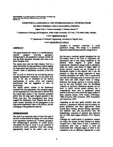
Fig. 1. Location and geography of the survey area.

necessary where there is a need for detailed assessment of the salt/freshwater distribution and estimates of e.g. chloride concentrations at the intake of water supply wells (Buckley et al., 2001; Mullen and Kellett, 2007), and where there is a need for determining the exact location of lithological boundaries. In this paper we present the results of a large AEM survey, which combined with seismic data and well logs provides an excellent picture of a series of subsurface structures as well as the salt/freshwater distribution in the survey area. The influence of these geological structures on the hydraulic system in response to future sea level rise is evaluated. The study emphasizes the need for sound representations of important geological features in numerical models and thus for the importance of having geophysical data available.

2 2.1

Area description Geography

The surveyed area covers the western part of the border region between Denmark and Germany (Fig. 1). The present-day landscape has been shaped by processes during Pleistocene and Holocene time. The morphology is mainly affected by undulating moraine hills preserved from the Saalian glaciations. The Weichselian outwash plains gently dip towards the flat Holocene marshland at the North Sea www.hydrol-earth-syst-sci.net/16/1845/2012/

coast. During the past 8000 yr, the marshland has been more or less covered by the North Sea with shallow salt-marsh deposition of mainly marine sand, but peat and gyttja are also present in the up to 10-m thick Holocene succession (Bartholdy and Pejrup, 1994; Hoffmann, 2004). Dike construction during the past 500 yr has converted the area into a dry, drained marshland (Jacobsen, 1964). According to the relief of the landscape, surface water runs off to the marshland from where it is channelled away to the North Sea by a dense net of drainage channels. The entire area has a rural character with cropland and grassland dominating the land use. 2.2

Hydrology and hydrogeology

The marshland is a low-lying area which has been developed into farmlands since the 16th century by the development of dikes and later drainage channels and pumping stations. The surface elevation in large parts of the area is around sea level (Fig. 2). To avoid inundation and to make these areas available for agriculture, they are drained through the channels. At numerous pumping stations, the water collected by the channels is pumped into the Vidaa River which routes the water to the North Sea. Because of the intensive drainage, the groundwater level in the upper aquifer does not exceed elevations of approximately one metre below soil surface, which corresponds to an elevation equal to or lower than sea level in a large part of the area. Hence, an inland hydraulic gradient is Hydrol. Earth Syst. Sci., 16, 1845–1862, 2012

1848


Fig. 2. Land surface elevation in metres above sea level (m a.s.l.), drainage system and groundwater abstraction.

established in a large area under present conditions that will slowly result in deterioration of the chemical status of the groundwater. The salinity in the subsurface of the marshland is generally high and above the WHO/EU drinking water standard of 250 mg l−1 , but it varies significantly with depth from about 40 mg l−1 to more than 3000 mg l−1 (Heck, 1931, 1932; GEUS, 2012; Ødum, 1934). Investigation wells and short wells within the marshland formerly used for households showed only shallow freshwater lenses directly resting on brackish groundwater (Ødum, 1934; GEUS, 2012); a situation that may be compared to the polder areas of Belgium (Vandenbohede et al., 2011) and the Netherlands (de Louw et al., 2011). Hence, groundwater abstraction wells are primarily installed at the margins of the marshland, e.g. the waterworks at the city of Tønder in Denmark and the city of Niebüll in Germany (Fig. 2). The quantity of groundwater abstraction at the well fields is relatively low: approximately 1.5 million m3 per year at Tønder and 3.0 million m3 per year at Niebüll; but local depressions in the hydraulic head distribution of the deeper aquifers are observed, which increases the risk of saltwater upconing. 2.3

Geology

The geology consists of three major sedimentary sequences (Fig. 3). Deep-marine Palaeogene clay is situated at depths Hydrol. Earth Syst. Sci., 16, 1845–1862, 2012

of about 300 m in the study area (Friborg and Thomsen, 1999). The Palaeogene clay is overlain by alternating layers of Miocene sand, silt and clay. The Miocene section consists of the deltaic Bastrup Formation, the marine clay formations of the fine-grained Klintinghoved and the more silty Arnum Formation overlain by the fine-grained Gram and Hodde Formations (Rasmussen et al., 2010). The clay formations are intervened by delta lobe sands. The Miocene sequence is covered by a relatively thin sheet of glacial sediments (10– 40 m). These glacial sediments can be considerably thicker in places where buried tunnel valleys incise Miocene and Palaeogene formations (Fig. 3) (Thomsen, 1990, 1991; Friborg and Thomsen, 1999; Jørgensen and Sandersen, 2006). The glacial sequence is mainly composed of coarse meltwater sediments, but clayey tills and glaciolacustrine clay occasionally also occur. A large-scale glaciotectonic thrust complex mapped in the Fanø Bugt 50 km towards the northwest is proposed to continue onshore through the survey area (Andersen, 2004). This complex is composed of kilometre-wide structures thrusted from easterly directions and with a basal décollement as deep as 200–360 m. Indications of glaciotectonics within the area (at Tønder) are also described on the basis of borehole data (Friborg, 1989). The complex is believed to have formed during the Saalian Warthe glaciation (Andersen, 2004; Houmark-Nielsen, 2007). Marine Eemian deposits are frequently found in boreholes along the coastal areas in the region (Friborg, 1996; Konradi

www.hydrol-earth-syst-sci.net/16/1845/2012/

g. 3


1849

Miocene

Incised tunnel valley

Pleistocene

Palaeogene Cretaceous Till Clay Sand Cret.

Fig. 3. Conceptual stratigraphical log for the survey area.

et al., 2005). The former Eemian shoreline is expected to have been situated more or less along the boundary between the marshland and the Pleistocene upland (Fig. 1). Since many borehole records show marine Eemian in and around the city of Tønder, it is proposed that a couple of palaeofjords may have reached some kilometres inland here (Friborg, 1996; Konradi et al., 2005). The survey area is transected by a NW–SE-striking fault zone (the Rømø Fault Zone) related to the evolution of the Ringkøbing-Fyn High (Cartwright, 1990). A graben structure (the Tønder Graben) has developed in the area along this fault zone and can be seen within the Palaeogene and Miocene setting (Friborg and Thomsen, 1999). It has been mapped in the survey area on the basis of conventional oil seismic data, but its precise outline and structure has only been roughly interpreted. A generalized stratigraphical log for the area is shown in Fig. 3.

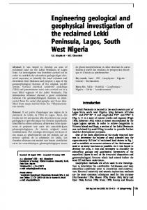
Fig. 4. Left: SkyTEM system. Right: example of a data curve divided into two moments, one giving information of the near-surface in the early times (Low Moment – LM) and the other one completing the sounding model in the deeper part with measurement at the late times (High Moment – HM).

the near surface and the other called High Moment (HM) which gives deep information (Fig. 4). These two moments are jointly inverted at each single sounding location estimating electrical resistivity from the near-surface to a depth of 250–300 m, depending on the setup used and the geology in the survey area. The height of the frame is measured by laser altimeter. To ensure correction for the movements of the frame, pitch/roll is continuously measured by inclinometers (Auken et al., 2009). With a nominal speed of 45 km h−1 and good weather conditions, the SkyTEM system has a production rate of 1000 km of flight lines within 4–5 days. 3.2

3 3.1

Methods SkyTEM

The SkyTEM system initially developed by Sørensen and Auken (2004) is a helicopter-borne time-domain AEM system that consists of a wire loop transmitter of a several hundred square metre area and of a small receiver loop of less than 1 m2 (Fig. 4). Different sizes of the transmitter loop exist depending on the depth of investigation required for a survey. The intensity of the current as well as the number of turns can also be increased to amplify the magnetic moment and thereby improve the signal-to-noise ratio and to get a larger depth of investigation. However, there is a trade-off since a higher current will induce a longer turn-off of the current inside the loop, which prevents the use of early times resulting in a poor near-surface resolution. For this reason, the SkyTEM usually operates with two transmitter moments, one called Low Moment (LM) which gives information on www.hydrol-earth-syst-sci.net/16/1845/2012/

Seismic

Seismic methods utilize differences in mechanical properties of geological units. The propagation velocity and signal strength of seismic waves inside earth depend on the dynamic elastic constants of the rocks and on their density. The method provides information primarily about the framework and delineation of geological units. Different types of waves are used for near-surface seismic surveying: compressional or P -waves and shear or S-waves that differ in depth range and resolution. Due to low velocity or impedance contrasts in the low, consolidated Quaternary or Neogene sediments present in the surveyed area, the refraction seismic method is not suitable. The reflection seismic systems used in this paper are appropriate for the target depths of 20 m to 700 m. The penetration depth is realizable with vibroseis and the common midpoint (CMP) method. With the P -waves used, the resolution is in the order of 4 m depending on wavelength and depth of target (Steeples, 2005).

Hydrol. Earth Syst. Sci., 16, 1845–1862, 2012

1850 3.3

F. Jørgensen et al.: Transboundary geophysical mapping of geological elements Borehole geophysics

A large number of different types of logging probes exist for measurements in boreholes. The different probes typically measure changes in the physical characteristics of the surrounding formation, which reflect changes in lithology and/or porewater salinity. The use of a combination of different geophysical logging probes, such as gamma (NG), induction (IN) and fluid temperature and conductivity (FTC), has proved very efficient for investigation of important characteristics of coastal aquifer systems (Buckley et al., 2001). These tools have therefore been used in the present study. The NG and IN tools reveal changes in the lithology of the formation surrounding the wells, while the FTC probe measures the temperature and electrical conductivity of the water inside the borehole, which generally represents an average of the conductivity of the porewater in the formation around the screened part of cased wells. Besides changes in the lithology of the formation, the IN logging probe also records detailed changes in the salinity of the porewater in the formation around the well, or rather a combination of changes in porewater hydrochemistry and formation lithology.

4 4.1

Surveys performed SkyTEM

A first survey was carried out in the German part north of the town of Niebüll during 17–25 September 2008 (west–east oriented lines in Fig. 5). This survey comprised 1481 line km with a line spacing of 250 m and covered an area of 396 km2 . The second survey was made in the Danish part around the town Tønder during 1–21 April 2009 (north–south oriented lines in Fig. 5). This survey included 1750 line km with a main line spacing of 166 m and covered an area of 325 km2 . The SkyTEM surveys utilized the largest SkyTEM loop with an area of 494 m2 and a maximum current for the HM of 95 A. This resulted in a larger penetration depth compared with other SkyTEM systems with smaller loops and lower currents. With a speed of 72 km h−1 for the Niebüll survey and a speed of 43 km h−1 for the Tønder survey, the average lateral resolution along the flight lines was about 25–30 m – at least for the first tens of metres from the surface. The resolution decreases with depth because of the diffusion of the electromagnetic signal with depth. The data were processed and inverted with the Aarhus Workbench software package (Viezzoli, 2009; Roth et al., 2011). The first step in the processing of the raw data was the removal of all coupling effects induced by man-made installations such as power lines, cables, pipes or railroads (Sørensen et al., 2001). Since these coupling effects cannot be modelled and compensated for, parts of flight lines affected by these couplings had to be removed from the data set. While automatic filtering can remove some of them, a Hydrol. Earth Syst. Sci., 16, 1845–1862, 2012

careful manual check had to be undertaken to remove both undetected couplings and remnants of only partly removed couplings. Once the couplings were removed from the raw data, the data were averaged with trapezoidal filters whose width increase with time after the turn-off of the source increased, i.e. as the data contain deeper and deeper information. These trapezoid filters were set in such a way that they were adapted to the signal-to-noise ratio which decreasinversion algorithm which give at late times. Finally, late time data were removed from averaged data where the background noise level reached the level of the earth response. Other filters on the altitude and the pitch/roll of the loop were also applied since these parameters influenced the strength of the recorded signal. After a final review of the data to check that all couplings were removed, the data were then inverted through a spatially constrained inversion algorithm which gave a quasi–3-D interpretation of the ground (Viezzoli et al., 2008, 2009). In this inversion procedure, the parameters of soundings were linked together with constraints that were proportional to the distance separating them. These constraints prevent artificial local results that may be due to poor signal-to-noise ratio and poorly defined parameters. However, care has to be taken when setting the strength of these lateral constraints which can induce overly smooth geological structures. To obtain a more realistic interpretation and to avoid problems due to a fixed number of layers, the sections were inverted into smooth models with 19 layers. The thicknesses of these layers were fixed. They increase logarithmically with the depth with the deepest layer boundary at 250 m. Their resistivity values were linked by vertical constraints to ensure smooth variations between the layers of the same sounding. 4.2

Seismic

A P -wave seismic reflection survey was conducted in May 2009 on the German side of the border by the Leibniz Institute for Applied Geophysics (LIAG). The survey was recorded with conventionally planted z-geophones (SM4 20 Hz) and LIAG’s vibrator truck in the area near Süderlügum (Fig. 5). With a 5-m receiver spacing and a 10m source spacing, a high-resolution subsurface image with a 2.5-m common midpoint (CMP) distance was obtained. For acquisition, LIAG used up to 264 channels in a combination of split spread and roll along techniques. Sourcereceiver offsets ranged from −1200 m to +1200 m. The maximum CMP fold was 129; the mean fold was at least 60. The hydraulic vibrator truck MHV2.7 (2.7 ton vibrator) was controlled by a sweep of 30–200 Hz with a length of 10 s and 4 sweeps were vertically stacked at each source point. The data were recorded with the Geometrics Geode system and saved in a stacked and correlated state. For quality control, several records with an impulse source (hammer blow) were taken. In total, 817 vibrator points on 7.8 km of profiles were www.hydrol-earth-syst-sci.net/16/1845/2012/


1851

Fig. 5. Map with SkyTEM data after processing (red lines) and seismic data (blue lines). The flight lines of the Tønder survey are north– south oriented. The flight lines of the Leck survey are west–east oriented. Seismic sections D2, D4 and G1–4 are shown in Figs. 6, 7 and 8. Unlabelled profiles were collected, but are not shown. SkyTEM profiles 1 and 2 indicated on the map are shown in Fig. 11. The locations of boreholes 167.711, 167.1538 and A49-3 are also shown.

recorded within 8 days. Five individual profile sections were acquired. On the Danish side of the border, five seismic reflection profiles were also surveyed. The profiles covered a total distance of 29.5 km and were recorded in April and May 2010 using an IVI Minivib T7000 3.5-ton vibrator and 224 towed 14 Hz L10 AI geophones in groups of two. The first group was used for recording the “pilot-trace” of the vibrator. The geophone trail wire length was 225 m. The first 49 active geophone groups were separated by 1.25 m, while spacing between each of the remaining 63 groups was 2.5 m. The source (vibro point) spacing was 10 m with a 6.25-m distance to the first active geophone group. Acquisition used Geometrics Seismodule Controller software and a 64-channel Geometrics StrataVisor instrument supplemented by two 24-channel Geometrics Geode recording units. At each source point, a minimum of two vibrator sweeps of 40–400 Hz with a length of 10 s were carried out. The data were collected and processed by Rambøll (2010).


The collected raw data show varying quality. The survey in the vicinity of Süderlügum profiles G1, G3 and G4 show a good signal/noise ratio, while profiles G2 and G5 were located near main roads and were influenced by cargenerated noise. The profiles north of the border were all located on roads with a limited amount of traffic, and the sections were therefore only to a minor extent influenced by traffic-generated noise. On the other hand, strong winds prevailing in the area were probably part of the reason for the insufficient quality on two profiles, D1 and D5. These two profiles were therefore resurveyed. Unfortunately, only D1 benefited from the effort. After geometry assignment, first breaks were picked and controlled with first breaks from the impulse source. Refraction statics were calculated from the first break picks and applied in the pre-stack processing. Additional steps performed included amplitude control by automatic gain control, spectral whitening and bandpass filtering, as well as trace-muting and application of residual statics. Velocity analysis provided stacking velocities for dip move-out (DMO) and normal move-out (NMO) correction Hydrol. Earth Syst. Sci., 16, 1845–1862, 2012

1852


and created seismic time sections after CMP stacking. In the post-stack processing, finite-difference time migration removed diffractions and F-X deconvolution smoothed the resultant section. Time-to-depth conversion finally created the depth sections that were used for interpretation. Stacking velocities were converted into interval velocities and an averaged single interval velocity function was used for time-todepth conversion. 4.3

Borehole geophysics

Three deep boreholes were logged in the study area: one well in Germany (A49-3, north of Karlum) and two in Denmark (archive no. 166.711 and 167.1538, GEUS, 2012; see Fig. 5 for locations). Two of the wells (A49-3 and 166.711) were logged by use of different geophysical probes including natural gamma (NG), induction (IN) and fluid temperature and conductivity (FTC). The logs were run at a speed of 3 m min−1 in either downwards (NG, FTC) or upwards direction (IN). The third well (167.1538) was logged in an open hole with drilling mud fluids; hence, the fluid conductivity log does not reflect the porewater conductivity. By using Archie’s law (Archie, 1942), it is possible to calculate the formation factor (the ratio between formation and porewater resistivity) from measurements of formation resistivity (by IN logs) and fluid resistivity (by FTC logs) through the screened section of a borehole. The formation factor is important when developing maps that provide a “regional” overview of the variations in groundwater resistivity (or conductivity), assessment of groundwater chloride concentrations and the chemical status in the investigated area. It is important to note that observed changes in formation resistivities may be the result of changes in either formation lithology or porewater salinity (or both). For example, a decrease in the IN log may stem either from increasing clay contents or from increasing porewater salinity. The only way to assess the relative importance of these factors is to use the NG log because the NG log remains unaffected by changes in porewater salinity, or by taking lithological information from sample descriptions into account. Lithological descriptions of borehole samples or the NG logs are therefore important for the correct interpretation of both IN logs and AEM measurements and, hence, the distribution of saltwater and the development of salt/freshwater interfaces in coastal aquifer systems. 5 5.1

Results Data interpretation

After processing and inversion, the geophysical data were subjected to geological interpretation. The use of borehole data is of utmost importance for successful transfer of acoustic and resistivity data into lithology and for spatial conceptualisation of the geological structures. Most borehole data Hydrol. Earth Syst. Sci., 16, 1845–1862, 2012

originate from water well construction, but also a few investigative drillings contribute to ground-truthing of the geophysical data. The available sample descriptions vary in quality, and care must be taken when they are used within the process of geological interpretation. They should generally be supported by geophysical borehole logs whenever possible. Furthermore, most of the boreholes are not very deep, typically less than 25–50 m, and they are too widely spaced to mimic spatial variations in the subsurface. The seismic data contribute detailed structural information along the 2D sections, but, again, even when combined with borehole data, there is no correlation between the sections in the area. The seismic data are displayed with borehole data (if deep boreholes are available within a reasonable distance from the section) and transparent colour-scaled SkyTEM data on top (Figs. 6, 7 and 8). This enables the interpreter to compare the structural information from the seismic data with the direct and derived lithological information from boreholes and SkyTEM. The SkyTEM resistivity data are converted into a series of horizontal slices each representing mean values at 5-m intervals. Resistivity values in these intervals are calculated for each SkyTEM smooth layer sounding model and subsequently interpolated using kriging with a horizontal cell size of 100 m. In order to allow detailed spatial inspection of the resistivity data, all grids from 250 m below the sea level (m b.s.l.) to the surface are stacked into a 3-D resistivity volume. This 3-D resistivity volume can be sliced horizontally at different levels (Figs. 9 and 10), but also vertically either along the seismic sections (Figs. 6, 7 and 8) or along any desirable profile section through the area (Fig. 11). During the process of geological interpretation, it is essential to do more than just evaluate interpolated resistivity data, because basic geophysical information is often lost in the transformation from sounding data to interpolated grids. The inverted resistivity models, dB/dt data, and data uncertainty must also be individually consulted on a regular basis in order to avoid misinterpretation due to noise, equivalence effects, resolution issues and structural heterogeneity, etc. The SkyTEM resistivity data are visualised through a colour scale where high resistivities are represented by reddish colours and low resistivities by blue colours. This is a widely used colour scale for electrical resistivity, and by using this in our coastal area, the seawater will be more intuitively imaged because it will occur in blue as hydrographic features generally do on maps. The following section will outline a series of prominent geological features that may be important in relation to future potential saltwater intrusion. 5.2

Faults

Faults related to the NW–SE-striking Rømø Fault Zone are clearly seen in the seismic profile D4 (Fig. 6). Two normal faults with offsets of 50–100 m are present on the section. www.hydrol-earth-syst-sci.net/16/1845/2012/


1853

Fig. 6. Interpreted seismic section (profile D4) with SkyTEM resistivity data showing the Tønder Graben with subsided Miocene and Palaeogene layers and a deep, buried tunnel valley. A new deep borehole (archive no. 167.1538, GEUS, 2012) drilled on the section is shown with lithological sample descriptions. The IN and NG logs obtained in the open well are shown on the section, too. For location of the section, see Figs. 5 and 9. Vertical exaggeration 3×.

Fig. 7. Interpreted seismic section (profile D2) with SkyTEM resistivity data showing glaciotectonised Miocene and Pleistocene layers and the same deep, buried tunnel valley as shown on profile D4. Lithology and an IN log from a borehole (archive no. 166.711, GEUS, 2012) located approximately 160 m in the eastward extension of the seismic section are also shown on the profile. Interference by bentonite plugs (shown on right of induction log) in this well produces false low-resistivity values at distinct intervals on the IN log, but an overall good match between the lithology and the log results is seen. For location of the section, see Figs. 5 and 10. Vertical exaggeration 3×.



1854


Fig. 8. Interpreted seismic section (profile G1–4) with SkyTEM resistivity data showing glaciotectonised Miocene and Pleistocene layers over an incised valley structure. For location of the sections, see Figs. 5 and 9. Vertical exaggeration 3×.

These faults bound a graben structure (the Tønder Graben) and intersect the entire setting until at least the Miocene. The Miocene Gram and Hodde clay (see section below) is subsided into a graben structure, and the faults must therefore have been active during or after the deposition of this clay. The southernmost fault seems to terminate into an incised tunnel valley (see section below), and the valley is therefore formed after the formation of the graben structure. The faults can also be laterally delineated in the resistivity data since the down-faulted Miocene clay is electrically very conductive. The clay layer is therefore distinct in the seismic section D4 (Fig. 6) and seen as a 75-m thick low-resistivity layer (8– 10 m) in the graben structure. By slicing the 3-D resistivity grid horizontally at levels around the subsided clay (100 to 175 m b.s.l.), the graben structure is delineated laterally by a low-resistivity elongated body (Fig. 9). The extent of the northern fault can also be traced in resistivity slices at higher levels (Fig. 10). Profile 1 in Fig. 11 shows an example of a S– N vertical slice through the 3-D resistivity volume. The faults bounding the graben structure are also clearly seen here (between profile coordinates 13 750 m and 16 000 m).


Fig. 9. Horizontal resistivity slice 152.5 m below sea level. Faults related to the Tønder Graben are shown with thick black lines. Grey lines depict the seismic lines shown in Figs. 6, 7 and 8. Location of the two SkyTEM profiles 1 and 2, shown in Fig. 11, are marked with dashed lines. Some of the deeper buried valleys are delineated, but not necessarily expressed in the resistivity data at this specific level.

5.3

Palaeogene and Miocene

An interpretation of oil seismic data has shown that the surface of the Palaeogene clay is generally situated at depths between 250 and 320 m b.s.l. outside the Tønder Graben; and inside the graben, it reaches depths of about 450 m b.s.l. (Friborg and Thomsen, 1999). A deep borehole (archive no. 167.1538, GEUS, 2012) situated exactly on the seismic section D4 (Fig. 6) shows that the top of the Palaeogene is situated at 325 m b.s.l., corresponding to a high amplitude reflection on the seismic section denoted by a blue line. The clay was found in the borehole samples and its exact location was confirmed by the NG log. This reflection can be traced on each of the seismic lines collected in the area. The reflection reaches depths of more than 500 m b.s.l. within the graben on section D4. The depth to the Palaeogene is generally too large to be resolved by the SkyTEM soundings. However, where it reaches its highest levels, towards the north and east, it is resolved as a very conductive layer (Fig. 11, profile 2). In these areas, it reaches about 200 m b.s.l. The Miocene deposits are primarily seen in the SkyTEM resistivity data as an upper conductive layer (8–10 m) and a lower resistive layer (>100 m). The upper layer, which is 50–75 m thick, is composed of marine Gram and Hodde www.hydrol-earth-syst-sci.net/16/1845/2012/


1855

Fig. 10. Horizontal resistivity slices at four selected levels. Mapped buried valleys are outlined on the maps, but not necessarily expressed in the resistivity data at each level. Boreholes with interglacial marine clay recordings are marked as black dots on 32.5 m below sea level. This particular valley was apparently inundated by the sea during the last interglacial. Location of the two SkyTEM profiles 1 and 2 shown in Fig. 11 are marked with dashed lines.

clay and occurs in areas where the glaciers did not remove or disturb it (buried valleys and glaciotectonics, see below). Where preserved, it is clearly portrayed in both vertical sections (profiles 1 and 2, Fig. 11). The layer is situated at levels of about 50 to 100 m b.s.l. in the eastern part, whereas it apparently gradually dips towards the west to a level of 100 to 150 m b.s.l. The lower resistive layer is mapped where the SkyTEM system is able to penetrate the Gram and Hodde clay layers (Fig. 11). According to Rasmussen et al. (2010), the less clayey marine Arnum Formation should be present below the Gram and Hodde clay in the survey area, followed by the deltaic sandy Bastrup Formation. The widespread


high-resistivity Miocene layers in the area (Figs. 6, 7, 8, 10 and 11) most likely correspond to sandy members of the Bastrup Formation. 5.4

Tunnel valleys

The area is dissected by a series of both deep and more shallow incisions whose appearance and property are typical for buried tunnel valleys in the area (Jørgensen and Sandersen, 2006, 2009). The deepest tunnel valley is seen on the two seismic sections D4 and D2 (Figs. 6 and 8). This valley reaches about 350 m b.s.l., but other valleys are much shallower. The valleys are precisely delineated in the resistivity Hydrol. Earth Syst. Sci., 16, 1845–1862, 2012

1856


South

Profile 1

Meltwater sand

Meltwater sand

2000

3000

4000

5000

6000

Miocene clay

Meltwater sand

Saline groundwater

Miocene silt/sand 1000

Glaciotectonic complex

Glaciolac. clay

Miocene clay

0

North Clay till

Clay till

7000

8000

9000

West

10000

km

Miocene silt/sand 11000

12000

13000

14000

15000

16000

17000

18000

19000

20000

East

Profile 2 Meltwater sand

e

e

lin 6000

8000

er

Miocene silt/sand?

er 4000

at

at

w

w

nd

2000

Miocene silt/sand

nd

ou

ou gr

Miocene clay

gr

0

Miocene clay

lin

Sa

Sa

Glaciotectonic complex

10000

12000

Paleogene clay 14000

16000

1

10

km

18000

Resistivity [Ωm]

20000

100

22000

24000

26000

28000

30000

32000

1000

Fig. 11. Cross section profiles through the SkyTEM 3-D resistivity grid: for location, see Figs. 5, 9 and 10. The deep valley seen in the seismic data on Figs. 6 and 7 is clearly seen on profile 1 (coordinate 10 000 m) where the Miocene clay is interrupted. The Tønder Graben structure is evident in the northern part of the profile. The area is partly capped by a thin sheet of clay till. Profile 2 shows the increased salinity in the western part, the dipping Miocene clay and one of the two glaciotectonically deformed areas. Vertical exaggeration 8 and 12×.

data (Fig. 10) because the resistivity of the infill typically differs from that of the surroundings. In some situations the valleys are filled with either glaciolacustrine clay or clay till, and they occur as elongated low-resistivity structures if incised into sandy Pleistocene or Miocene sediments. In other situations, they are filled with coarse glaciofluvial deposits, and in such cases they occur as resistive structures. The valleys are typically visible at different levels along their pathways (Fig. 10). Their widths vary from a few hundred metres to about 2.5 km. As mentioned, the infill is composed of a variety of Pleistocene sediments. Profile D2 (Fig. 7) shows thick, high-resistivity sediments in the lower part of the valley covered by a 25–50-m thick layer of low-resistivity sediments. Above this, high-resistivity sediments are found again, and the entire sequence is capped by a thin lowresistivity layer. According to borehole 166.711 (see lithology and IN log, Fig. 7), the high-resistivity sediments correspond to glacial meltwater sand, whereas the low-resistivity layer corresponds to glaciolacustrine clay and silt. The lowresistivity top layer corresponds to clay till. Approximately the same overall setting is seen in the same valley in profile 1 (Fig. 11, profile coordinate 9500–11 500 m). The valley is also crossed by section D4, but the drilling here (167.1538) shows a thicker sequence of fine-grained meltwater sediments (Fig. 6). The IN log, however, indicates that the upper parts of this sequence are more resistive and are therefore likely to be more silty than the lower part. A distinct drop in formation resistivity to about 5 m is seen for the lower part of the valley sediments in the IN log. Since lithologic logs describe the sediments as mainly sandy at this depth, low resistivity suggests that the formation must be affected by saline porewater here. This corresponds to the low resistivities as measured by the SkyTEM (Fig. 6).


The deep valleys typically cut through the Miocene clay layers and into the deep sandy/silty Miocene layers (Figs. 6, 7, 8 and 11). Apparently, they do not follow the fault Fig.struc11 tures and seem therefore to be unaffected by their presence (Fig. 9). All boreholes hosted in the Danish national borehole database (GEUS, 2012) have been searched for records of Eemian deposits throughout the area, and boreholes with hits are plotted on the uppermost horizontal slice in Fig. 10. It appears that there is a good match between the outline of one of the buried valleys and the occurrence of Eemian deposits. It is likely that this particular valley was open and inundated by the sea during the last interglacial. The mapped valley therefore constitutes one of the palaeo-fjords proposed by Friborg (1996) – the Tønder Fjord. On top of the marine Eemian, the valley is filled by meltwater sediments from the Weichselian glaciation (Konradi et al., 2005), and it is therefore not visible in present-day topography. The precise time of incision of the valley is uncertain, but a Saalian age is likely since it was open during the Eemian. The age of the other valleys is unknown, but it is possible that at least the deep valley seen on profiles D2 and D4 (Figs. 6 and 7) is older than the Late Saalian, because it is situated below the Saalian moraine hill north of Tønder (Fig. 1) which is covered by Late Saalian till. The general pattern of the valleys indicates more than one single valley generation. Apparently, there are NE–SW oriented valleys, N–S oriented valleys and one SE–NW oriented valley – probably three generations. 5.5

Glaciotectonics

The SkyTEM data show a very heterogeneous picture in two distinct areas (labelled “Glaciotectonic complex” in Fig. 10). www.hydrol-earth-syst-sci.net/16/1845/2012/

F. Jørgensen et al.: Transboundary geophysical mapping of geological elements These areas are situated in the central northern part and in the central southern part of the survey area. The areas generally appear as more resistive, but they are interrupted by many small, often slightly elongated low-resistivity bodies. The seismic lines D2 and G1–4, all collected in these areas, indicate the presence of folds and thrust structures with a décollement between 150 and 200 m b.s.l. (marked by a black line in Figs. 7 and 8). It is therefore inferred that the heterogeneous areas express the extent of one or two large glaciotectonic complexes. The elongated low-resistivity bodies seen in the resistivity data are mainly SE–NW oriented, which indicates an ice movement from a northeasterly direction. This is more or less consistent with the findings in the Fanø Bugt, where the large glaciotectonic complex was formed by a glacier from the east (Andersen, 2004). It is therefore plausible that the complexes found in our survey are an onshore continuation of the larger offshore complex as also proposed by Andersen (2004). If this is true and the assumed Late Saalian age of the complex is true, then at least the deep, buried tunnel valley depicted on the seismic sections D2 and D4 (Figs. 6 and 7), which is older than Late Saalian, must have been exposed to the glaciotectonic stress. Strongly dipping and wavy reflections, which may represent glaciotectonic deformation within the valley fill, are seen between 2000 and 3500 m on profile D4, and between 2500 and 3500 m on profile D2 (Fig. 7), but this interpretation is uncertain. On the other hand, a relatively clear erosional boundary between the valley and the surroundings indicates that the valley infill was not severely deformed by glaciotectonic deformation. Indications of an old incision below the décollement plane (Fig. 8) are seen on the seismic profile G1–4. The profile shows the pre-existence of a valley before the glaciotectonic deformation took place. Thus, it is difficult to assess the exact chronology of valley incision and glaciotectonic deformation, but the valley incision likely occurred both before and after the deformation phase. 5.6

Formation resistivity, formation factors, groundwater salinity and chemical status

The saltwater-saturated subsurface of the low-lying marshland is clearly depicted in the resistivity data, which generally shows low resistivities here. The area with low resistivities in the southwestern part of the survey area (as seen in Fig. 10, 32.5 m b.s.l.) corresponds to the extent of the marshland (Fig. 1). Although the setting is saturated with saltwater, it is still possible to delineate the buried valleys and the Miocene layers in the maps and on the cross sections (Figs. 10 and 11, profile 2). The resistivity of the Miocene silt/sand is seen to be considerably lower than in the freshwater-saturated areas, but resolution problems prevent assessment of the exact resistivity value that deep in the conductive setting, which acts as an effective shield. The resistivity of the assumed Miocene clay is somewhat lower www.hydrol-earth-syst-sci.net/16/1845/2012/

1857

(3–5 m at profile coordinate 0–14 000 m, profile 2, Fig. 11) than in the freshwater-saturated setting (5–7 m at profile coordinate 26 000–32 000 m, profile 2, Fig. 11). Above the Miocene clay layer in the saltwater-saturated area (Fig. 11, profile 2), the setting can generally be subdivided into three layers based on its resistivity. Although it is still rather low, a layer with a relatively high resistivity (∼6–8 m) exists right above the assumed clay. This layer is overlain by a low-resistivity layer (∼2–4 m) which is topped by a shallow near-surface layer (0–10 m depth) that sometimes has relatively high resistivities. The last layer’s high-resistivity spots are probably identical to the areas with shallow lenses of freshwater and old drinking water wells. The resistivity of the second layer is higher than expected for sediments saturated by seawater originating from the North Sea. The formation factor is estimated for the wells 166.711 and A49-3 (see Fig. 5 for location) to be 3.5 and 3.1, respectively, for the screened sandy sections of the wells. This compares well with the average formation factor (3.4, std. 0.5) estimated from 19 well logs in coastal sandy aquifers in Belgium, The Netherlands, Germany and Denmark performed as part of the CLIWAT project, and with assessments of the average formation factor (3.5) in sandy aquifers at the Belgian coast line (Vandenbohede et al., 2011). With a typical resistivity for seawater of 0.3 m, the resulting formation resistivity would be approximately 1.0 m (Archie, 1942). A previous study reported a resistivity of 1 m in a borehole log from the northern part of the island of Rømø (archive no. 148.52) in the northern part of the Wadden Sea (Hinsby et al., 2001); and true seawater salinities were confirmed by chemical groundwater analysis at the relevant level. Since the resistivity reaches 6–8 m in the investigated area, the sediments do not seem to be saturated with fully marine sea water. The same reasoning applies to the Miocene clay layer and the upper low-resistivity layer. These layers do not reach such low resistivity values either, and the sediments are therefore not saturated with fully marine sea water. A couple of flight lines over the tidal flat on the seaside of the dike also show resistivity values above the expected level for sediments saturated by fully marine water (Fig. 10). Assuming an average formation factor of 3.5, the porewaters of the sandy aquifers in the region breach the EU drinking water guideline for electrical conductivity (250 ms m−1 = 4 m) when the AEM and/or borehole log measurements show formation resistivities below 14 m (3.5 × 4 m). Similarly, in analogy with a suggested European threshold value for chloride (Hinsby et al., 2008), the threshold value for electrical conductivity would be 150 ms m−1 or 23 m (3.5 × (1/0.15)). Hence, sandy aquifers in the investigated region with resistivities below approximately 23 m contain groundwater of poor chemical status according to the EU groundwater directive.


1858 6


Hydrogeological evaluation and discussion

The results from the survey show that large parts of the area are affected by saltwater. The saltwater observed in the Miocene aquifers may be residual from the time when the formation was deposited, saltwater either flushed into the system during Pleistocene or Holocene transgressions, or it intruded in recent times after dike construction and drainage of the marshland. Since saltwater is not found in the Miocene sediments bordering on the marshland, it is likely that the residual saltwater had been flushed by freshwater during periods where the sea levels were much lower than the present, e.g. during the Last Glacial Maximum where the sea level was more than 120 m lower than now (Edmunds et al., 2001; Clark and Mix, 2002). The origin of the saltwater is therefore expected to be more recent, either due to infiltration and intrusion during the Holocene transgression and/or as a result of seawater intrusion after the drainage of the area. Based on the current knowledge, however, it is difficult to make further estimates of the origin of the saltwater. The dynamics of the saltwater are also difficult to assess, i.e. if residual saltwater is presently being flushed by freshwater, or if the present drainage and pumping in the area generates additional saltwater intrusion into the aquifers. However, the low resistivities seen in Fig. 11, profile 2 between coordinates 0 and 12 000 m indicate that flushing of the saltwater is not taking place or is very low in the current situation. Only the uppermost about 10 m show high resistivities indicating that freshwater is restricted to the shallow aquifer system. Hence, freshwater lenses have probably developed between the drainage channels in the polder area in response to infiltrating rainwater and upward flowing saline groundwater (de Louw et al., 2011), which indicates that the system is not in a situation of refreshing. As mentioned above, the resistivities of the formations in the marshland area (Fig. 11, profile 2) are higher than expected for sediments saturated with fully marine water. Hence, the salinities of both the Miocene clay and the sandy Miocene and Pleistocene deposits above are below that of the North Sea, which indicates that dilution has taken place. Such conditions have also been reported from Rømø where partly flushed seawater (brackish water) was also found at a depth of 300 m and below more than 100 m of marine clays in well 148.52 (Hinsby et al., 2001). Due to density differences, rainwater from above is not expected to recharge deep into the profile. The reduced salinities may therefore be caused by an upward flow of fresher water from below. Active groundwater flow may take place from east to west through the deep Miocene sediment seen on Fig. 11, profile 2, between the coordinates of 0 and 14 000 m at elevations below −150 m. This aquifer is probably fed by groundwater recharging in the central part of Jutland (Hinsby et al., 2001), which is known to be an artesian aquifer. Unfortunately, measurements of hydraulic head from the deep part of the Miocene aquifer are only available at a few locations, Hydrol. Earth Syst. Sci., 16, 1845–1862, 2012

including archive no. 158.698 and 159.995 (GEUS, 2012) located 15 km north and 14 km northeast of Tønder, respectively, where head values above soil surface have been observed. The hydraulic heads of this formation may therefore be higher than the equivalent freshwater heads of surficial sandy formations intruded by sea water. In this case, groundwater is expected to seep up through the clay layer and further up through the sand layer due to buoyancy forces. Such a mechanism could give rise to salinities that are lower than those corresponding to fully marine conditions and could explain the observed elevated resistivities. The existence of an active flow system in the lower Miocene sand/silt formation could also explain the relatively high resistivities found in the deeper parts of the buried valley seen on Fig. 11, profile 2, between coordinates 1000–1500 m and in Fig. 9 at a depth of 152.5 m. The existence of fresh water below the more saline water in the valley probably requires that (1) the infill of the valley is layered in a manner that partially confines the lower part from the upper saline part and (2) that the flux of fresh groundwater through the lower part is sufficient to dilute the buoyancy-driven downward flux of high-salinity water from above. If these requirements are met, the buried valley may act as a drainage channel for the deep Miocene aquifer. This hypothesis is corroborated by the fact that the Miocene sand formations tend to pinch out close to the west coast of Jutland (Scharling et al., 2009), in which case the flow through the formations is restricted. However, as the layered Miocene sequence seems to have been destroyed by the formation of the glaciotectonic complex just to the east of the marshland (Fig. 11), the Miocene clay may not be very effective as a confining layer in this area. The hypothesis discussed above is therefore only tentative and it requires that the confining layer is uninterrupted by glaciotectonics or by other elements such as tunnel valleys. Low resistivities likely to represent saline groundwater are also found on profile 1 (Fig. 11) between coordinates 6000 and 7000 m next to the marshland. They are found in the Miocene silt/sand at a location exactly below one of the tunnel valleys that perforates the Miocene clay. This area was not inundated by the Holocene transgression, but the tunnel valley was an open fjord during the Eemian (Fig. 10) and during this period the saline groundwater may have infiltrated through the valley to the underlying Miocene sand and silt layers. If seawater intruded through the valley during the Eemian, there should be no groundwater flow in the aquifer since the seawater body still exists. This contradicts the hypothesis discussed above, where flow was expected to take place in the lower Miocene aquifer. Another possibility is therefore that the valley is deeper than may be anticipated from the SkyTEM data (as drawn on Fig. 10) and that the observed low resistivities originate from clay sediments and/or saltwater within the valley itself. If the latter is true and the valley hosts saltwater, the water could perhaps have intruded laterally from the North Sea through the valley infill.


F. Jørgensen et al.: Transboundary geophysical mapping of geological elements Unfortunately, there are no boreholes, logs or seismic data to clarify this question. The continuation of the tunnel valleys towards the North Sea through the marshland is evidenced by elongated bodies with resistivity values that deviate from those of their surroundings (Figs. 10 and 11). In the uppermost 60 m, the southwestward continuation of the above-mentioned Eemian valley exposes resistivities in the vicinity of around 2–3 m, and in the southwestern-most part close to the North Sea the resistivities are between 1 and 2 m. Thus, unlike the surrounding sediments, the valley may here host full marine water. This water could be remnants of old marine water, but the observed difference in resistivities could also point to the fact that the valleys act as pathways for past and/or present seawater intrusion into the marshland. As described above, the hydrogeology of the study area is very complex, and detailed predictions of the impact of a sea level rise are therefore difficult to make. The complex geological setting and hydrological flow system only allow tentative evaluations. Due to the drainage system in the marshland, the groundwater table is here located close to or below the sea level. Hence, a hydraulic gradient from the sea towards the inland areas exists in the present conditions. Saltwater is therefore expected to migrate into the inland aquifers. Since the groundwater table is controlled by the drainage and pumping systems, a rise in the sea level will not affect the elevation of the groundwater table in the marshland. Hence, a higher sea level is expected to result in a higher gradient and therefore increasing saltwater intrusion (Werner and Simmons, 2009), at least in the upper aquifers. Hansen et al. (2011) show that isostatic down-warping at a rate of 0.25–0.50 mm yr−1 takes place in the border region of Denmark and Germany. In combination with eustatic sea level rise, this makes the area especially vulnerable to sea water intrusion. If the geology in the area was not interrupted by faults, buried valleys and glaciotectonics, the relatively thick and widespread Miocene clay layer would be continuous and would cover a large area from central Jutland into the North Sea. In this case, the aquifer in lower Miocene sand/silt (Fig. 11) would be confined and would presumably not be intruded by seawater as it would be protected by the overlying clay layer. However, the geological anomalies do provide pathways between the upper Quaternary aquifers and the Miocene aquifers in the area, as sea–aquifer exchange usually takes place along preferential pathways (Carrera et al., 2010). Density-driven convective flow may take place at these locations which will result in saltwater intrusion into the deeper aquifers. Head gradients caused by groundwater abstraction from the Miocene aquifers, e.g. at Tønder and Niebüll, may enhance this development. An example is seen at the Tønder Graben where it is likely that the upper aquifers are in hydraulic contact with the lower Miocene aquifer (Figs. 9 and 11) and therefore may serve as a pathway for saline water in the area close to the sea. A similar www.hydrol-earth-syst-sci.net/16/1845/2012/

1859

situation has been described by Nishikawa et al. (2009). The glaciotectonic complex seen in Fig. 11, profile 2 may constitute another structure where downward migration of saltwater may take place if sea water intrudes further into the upper aquifer, e.g. at coordinates 12 000–14 000 m. Even more critical for the exchange of saline groundwater between aquifers may be the frequent occurrence of incised and cross-cutting buried tunnel valleys (Figs. 6, 7, 10 and 11). The east–west-aligned buried tunnel valleys connecting the sea aquifers and the Miocene aquifers through the marshland, as well as further inland, constitute elements central for the horizontal exchange of water. They often contain coarsegrained and highly permeable infills that allow for immense vertical exchange between the upper and the lower Miocene sand layers. Since the valleys cross-cut and since they often contain more than one aquifer (like the deep valley shown in Figs. 6 and 7), exchange may also take place between different valley aquifers in the same or different valleys. It is therefore very important not only to map the valleys, but also to know the age relationships between cross-cutting valleys (and other geological elements). In our study, we have estimated the age relationships between different buried valleys and the glaciotectonic complex, but a number of questions regarding this issue remain unanswered. The exchange of groundwater between aquifers hosted in the different geological structures is very likely to play an important role for the entire flow regime in the area and would probably be enhanced by the increased potential gradients due to a rising sea level. A qualitative evaluation of the impact of geological structures on saltwater migration in the study area has been presented above. A quantitative assessment of the risk of saltwater intrusion in response to a sea level rise requires the use of a comprehensive density-dependent flow and transport model. In addition, a reliable prediction of the exchange of saltwater between the sea and the inland aquifers and between the different formations requires a detailed 3-D geological model. In such a model, it is of paramount importance to incorporate the interpreted geological elements as they have been described in the present paper. A flow model would perhaps be able to give answers to some of the many open questions about the flow system and the exchange between aquifers, but since the described geological elements are critical for the entire flow regime and thus for the flow calculations, these elements have to be properly characterised both spatially and lithologically. It is questionable whether this task has been sufficiently fulfilled by the present investigation because a series of basic questions remain open. These questions relate, for instance, to the extension and the lithology of the lower Miocene aquifer; to the occurrence, spatial extent and age relationships of the buried valleys; to the lack of spatial resolution of the interior of the glaciotectonic complex; and to difficulties of mapping all fault structures precisely in the entire area. On the other hand, it is evident from this study that it would not be Hydrol. Earth Syst. Sci., 16, 1845–1862, 2012

1860


possible to perform a modelling exercise in this area without geophysical data. Such data must include densely collected resistivity data, which, combined with borehole logs, provide an indispensable spatial overview of the geological structure and salinity distribution as well as the lithological properties of the area. In addition, seismic data may provide a detailed structural picture of the subsurface. In order to answer the open questions and thus to be able to establish and conduct unambiguous density-dependent flow and transport modelling, additional data collection would most likely be required. Particular benefit would also accrue from access to seismic data as well as borehole data and well logs, and also information on hydraulic head, salinity and groundwater age at selected locations, especially from the deeper aquifers. Such data are important for a full and integrated understanding of the flow dynamics and hydrochemical evolution in groundwater systems (Gannon et al., 2012), not least when the groundwater systems are closely linked to the sea (Vandenbohede et al., 2011). 7

Conclusions

We have conducted a geological, physical and hydrochemical characterisation of the subsurface by a combination of airborne, surface and borehole geophysics and geological well logs in a transboundary study in the border region between Germany and Denmark. Furthermore, we have illustrated and discussed the importance of a sound understanding and description of the subsurface, including the hydraulic parameters which are of crucial importance for accurate predictions of the impacts of climate change and sea level rise in coastal regions. Detailed descriptions of geologically important features, such as buried valleys and fault zones and their hydraulic characteristics, are of vital importance for the assessment of the impacts of climate change and sea level rise.

Acknowledgements. The study is a part of the CLIWAT project, which is co-funded by The Interreg IVB North Sea Region Programme, European Union. The manuscript was greatly improved by reviews from M. Deszcz-Pan, J. Ehlers and by editorial comments from B. Siemon. Edited by: B. Siemon

References Andersen, L. T.: The Fanø Bugt Glaciotectonic Thrust Fault Complex, Southeastern Danish North Sea. A study of large-scale glaciotectonics using high-resolution seismic data and numerical modeling, Ph.D. thesis, Department of Earth Science, Aarhus University, Geological Survey of Denmark and Greenland report 2004/30, 2004. Andersen, M. S., Baron, L., Gudbjerg, J., Gregersen, J., Chapellier, D., Jakobsen, R., and Postma, D.: Discharge of nitrate-containing


groundwater into a coastal marine environment, J. Hydrol,, 336, 98–114, 2007. Archie, G. E.: The electrical resistivity log as an aid in determining some reservoir characteristics, T. Am. I. Min. Met., 146, 54–62, 1942. Auken, E. and Sørensen, K. I.: Large-scale TEM investigation for groundwater ASEG, Australia, 2003. Auken, E., Christiansen, A. V., Westergaard, J. A., Kirkegaard, C., Foged, N., and Viezzoli, A.: An integrated processing scheme for high-resolution airborne electromagnetic surveys, the SkyTEM system, Explor. Geophys., 40, 184–192, 2009. Auken, E., Foged, N., and Sørensen, K. I.: Approaching 10 microsec (and earlier) with the SkyTEM system ASEG, 21st International Geophysical Confernce and Exhibition, Sydney, 2010a. Auken, E., Kirkegaard, C., Ribeiro, J., Foged, N., and Kok, A.: The use of airborne electromagnetic for efficient mapping of salt water intrusion and outflow to the sea, SWIM21 – 21st Salt Water Intrusion Meeting, 21–26 June, Azores, Portugal, 2010b. Bartholdy, J. and Pejrup, M.: Holocene Evolution of the Danish Wadden Sea, Senck. Marit., 24, 187–209, 1994. Bear, J., Cheng, A. H. D., Sorek, S., Ouazar, D., and Herrera, I.: Seawater intrusion in coastal aquifers – concepts, methods and practices, Kluwer Academic Publishers, Dordrecht, 1999. Buckley, D. K., Hinsby, K., and Manzano, M.: Application of geophysical borehole logging techniques to examine coastal aquifer palaeohydrogeology, Geol. Soc. SP, 189, 251–270, 2001. Calvache, M. L. and Pulido-Bosch, A.: Effects of geology and human activity on the dynamics of salt-water intrusion in three coastal aquifers in southern Spain, Environ. Geol., 30, 215–223, 1997. Carrera, J., Hidalgo, J. J., Slooten, L. J., and Vázquez-Suñe´ , E.: Computational and conceptual issues in the calibration of seawater intrusion models, Hydrogeol. J., 18, 131–145, 2010. Cartwright, J.: The structural evolution of the Ringkøbing-Fyn High, in: Tectonic Evolution of the North Sea Rifts, edited by: Blundell, D. J. and Gibbs, A. D., Clarendon Press, Oxford, 200– 216, 1990. Chang, S. W., Clement, T. P., Simpson, M. J., and Lee, K.-K.: Does sea-level rise have an impact on saltwater intrusion?, Adv. Water Resour., 34, 1283–1291, 2011. Clark, P. U. and Mix, A. C.: Ice sheets and sea level of the Last Glacial Maximum, Quaternary Sci. Rev., 21, 1–7, 2002. Custodio, E. and Bruggeman, G. A.: Groundwater problems in coastal areas, UNESCO, International Hydrological Programme, Paris, 1987. de Louw, P. G. B., Eeman, S., Siemon, B., Voortman, B. R., Gunnink, J., van Baaren, E. S., and Oude Essink, G. H. P.: Shallow rainwater lenses in deltaic areas with saline seepage, Hydrol. Earth Syst. Sci., 15, 3659–3678, doi:10.5194/hess-15-36592011, 2011. Edmunds, W. M., Hinsby, K., Marlin, C., Condesso de Melo, M. T., Manzano, M., Vaikmae, R., and Travi, Y.: Evolution of groundwater systems at the European coastline, Geol. Soc. SP, 189, 289–311, 2001. Fitterman, D. V. and Deszcz-Pan, M.: Characterization of Saltwater Intrusion in South Florida Using Electromagnetic Geophysical Methods, Proceedings of the 18th Salt Water Intrusion Meeting, 31 May–3 June 2004, Cartagena, Spain, 2004.


F. Jørgensen et al.: Transboundary geophysical mapping of geological elements Friborg, R.: Geologisk model for Tønder Nyhedsbrev, May 1989, Sønderjyllands Amt, 1989. Friborg, R.: The landscape below the Tinglev outwash plain. A reconstruction, B. Geol. Soc. Denmark, 43, 34–40, 1996 Friborg, R. and Thomsen, S.: Kortlægning af Ribeformationen. Et fællesjysk grundvandssamarbejde, Technical report, Ribe ˚ Amt, Ringkøbing Amt, Viborg Amt, Arhus Amt, Vejle Amt, Sønderjyllands Amt, ISBN no. 87-7486-359-2, 1999. Gannon, J. P., Burbey, T. J., Bodnar, R. J., and Aylor, J.: Geophysical and geochemical characterization of the groundwater system and the role of Chatham Fault in groundwater movement at the Coles Hill uranium deposit, Virginia, USA, Hydrogeol. J., 20, 45–60, 2012. GEUS: The National well database (Jupiter), available at: http://geuskort.geus.dk/GeusMap/index jupiter.jsp?imgxy= 622+403&iMapWidth=1244&iMapHeight=806, last access: 15 February 2012. Hansen, J. M., Aagaard, T., and Binderup, M.: Absolute sea levels and isostatic changes of the eastern North Sea to central Baltic region during the last 900 years, Boreas, online first: doi:10.1111/j.1502-3885.2011.00229.x, 2011. Heck, H.-L.: Grundwasserverhältnisse und geologischer Bau im schleswig-holsteinischen Marsch- und Nordseeinselgebiet, Sitzungsber. D. Preuss. Geol. Landesanstalt, 6, 169–196, 1931. Heck, H.-L.: Das Grundwasser im Zusammenhang mit dem geologischen Bau Schleswig-Holsteins, Preuss. Geol. Landesanstalt, 133 pp., 1932. Hinsby, K., Harrar, W. G., Nyegaard, P., Konradi, P. B., Rasmussen, E. S., Bidstrup, T., Gregersen, U., and Boaretto, E.: The Ribe Formation in western Denmark; Holocene and Pleistocene groundwaters in a coastal Miocene sand aquifer, Geol. Soc. SP, 189, 29–48, 2001. Hinsby, K., de Melo, M. T. C., and Dahl, M.: European case studies supporting the derivation of natural background levels and groundwater threshold values for the protection of dependent ecosystems and human health, Sci. Total Environ., 401, 1–20, 2008. Hoffmann, D.: Holocene landscape development in the marshes of the West Coast of Schleswig-Holstein, Germany, Quaternary Int., 112, 29–36, 2004. Houmark-Nielsen, M.: Extent and age of Middle and Late Pleistocene glaciations and periglacial episodes in southern Jutland, Denmark, B. Geol. Soc. Denmark, 55, 9–35, 2007. Høyer, A., Lykke-Andersen, H., Jørgensen, F., and Auken, E.: Combined interpretation of SkyTEM and high-resolution seismic data, Phys. Chem. Earth, 36, 1386–1397, 2011. IPCC: Climate Change 2007 – The Physical Science Basis. Contribution of Working Group I to the Fourth Assessment Report of the Intergovernmental Panel on Climate Change 2007: Synthesis Report. Contribution of Working Groups I, II and III to the Fourth Assessment. Report of the Intergovernmental Panel on Climate Change, edited by: Pachauri, R. K. and Reisinger, A., IPCC, Geneva, Switzerland, 104 pp., 2007. Iribar, V., Carrera, J., Custodio, E., and Medina, A.: Inverse modelling of seawater intrusion in the Llobregat delta deep aquifer RID E-7251-2011, J. Hydrol., 198, 226–244, 1997. Jacobsen, N. K.: Tøndermarskens Naturgeografi, Folia Geogr. Danm., 7, 350 pp., 1964.


1861

Jørgensen, F. and Sandersen, P. B. E.: Buried and open tunnel valleys in Denmark – erosion beneath multiple ice sheets, Quaternary Sci. Rev., 25, 1339–1363, 2006. Jørgensen, F. and Sandersen, P. B. E.: Buried valley mapping in Denmark: evaluating mapping method constraints and the importance of data density. Z. Dtsch. Ges. Geowiss., 160, 211–223, 2009. Jørgensen, F., Lykke-Andersen, H., Sandersen, P. B. E., Auken, E., and Nørmark, E.: Geophysical investigations of buried Quaternary valleys in Denmark: An integrated application of transient electromagnetic soundings, reflection seismic surveys and exploratory drillings, J. Appl. Geophys., 53, 215–228, 2003. Kafri, U. and Goldman, M.: The use of the time domain electromagnetic method to delineate saline groundwater in granular and carbonate aquifers and to evaluate their porosity, J. Appl. Geophys., 57, 167–178, 2005. Kirkegaard, C., Sonnenborg, T., Auken, E., and Jørgensen, F.: Salinity distribution in heterogeneous coastal aquifers mapped by airborne electromagnetics, Vadose Zone J., 10, 125–135, 2011. Kok, A., Auken, E., Groen, M., Ribeiro, J., and Schaars, F.: Using Ground based Geophysics and Airborne Transient Electromagnetic Measurements (SkyTEM) to map Salinity Distribution and Calibrate a Groundwater Model for the Island of Terschelling – The Netherlands 21st SWIM conference, Azores, 2010. Konradi, P. B., Larsen, B., and Sørensen, A. B.: Marine Eemian in the Danish eastern North Sea, Quaternary Int., 133–134, 21–31, 2005. Mullen, I. and Kellett, J.: Groundwater salinity mapping using airborne electromagnetics and borehole data within the lower Balonne catchment, Queensland, Australia, Int. J. Appl. Earth Obs., 9, 116–123, 2007. Mulligan, A. E., Evans, R. L., and Lizarralde, D.: The role of paleochannels in groundwater/seawater exchange, J. Hydrol., 335, 313–329, 2007. Nishikawa, T., Siade, A. J., Reichard, E. G., Ponti, D. J., Canales, A. G., and Johnson, T. A.: Stratigraphic controls on seawater intrusion and implications for groundwater management, Dominguez Gap area of Los Angeles, California, USA, Hydrogeol. J., 17, 1699–1725, 2009. Nyboe, N. S., Jørgensen, F., and Sørensen, K. I.: Integrated inversion of TEM and seismic data facilitated by high penetration depths of a segmented receiver setup, Near Surf. Geophys., 8, 467–473, 2010. Ødum, H.: Grundvandsforholdene i Tønder-Marsken, DGU, IV rk., 2, 17 pp., 1934. Oude Essink, G. H. P.: Salt water intrusion in a three-dimensional groundwater system in the Netherlands: A numerical study, Transport Porous Med., 43, 137–158, 2001. Oude Essink, G. H. P., van Baaren, E. S., and de Louw, P. G. B.: Effects of climate change on coastal groundwater systems: A modeling study in the Netherlands, Water Resour. Res., 46, W00F04, doi:10.1029/2009WR008719, 2010. Post, V. and Abarca, E.: Preface: Saltwater and freshwater interactions in coastal aquifers RID E-6054-2011, Hydrogeol. J., 18, 1–4, 2010. Rambøll: Seismisk kortlægning ved Tønder, Unpublished report, 2010. Rasmussen, E. S.: Detailed mapping of marine erosional surfaces and the geometry of clinoforms on seismic data: a tool to identify


1862


the thickest reservoir sand, Basin Res., 21, 721–737, 2009. Rasmussen, E. S., Dybkjær, K., and Piasecki, S.: Lithostratigraphy of the Upper Oligocene – Miocene succession of Denmark, Geol. Surv. Den. Greenl., 22, 92 pp., 2010. Ribeiro, J.: Interaction of salt – fresh water using airborne TEM methods, Faculty of Science – Lisbon University, 2010. Roth, B., Mikkelsen, P., and Auken, E.: SkyTEM Survey Tønder 2009, Leck 2008, Rens/Løgumg˚arde 2011, Department of Earth Sciences, Aarhus University, 2011. Rumpel, H.-M., Binot, F., Gabriel, G., Siemon, B., Steuer, A., and Wiederhold, H.: The benefit of geophysical data for hydrogeological 3D modelling – an example using the Cuxhaven buried valley, Z. Dtsch. Ges. Geowiss., 160, 259–269, 2009. Sandersen, P. B. E., Jørgensen, F., Larsen, N. K., Westergaard, J., and Auken, E.: Rapid tunnel valley formation beneath the receding Late Weichselian ice sheet in Vendsyssel, Denmark, Boreas, 38, 834–851, 2009. Schamper, C., Auken, E., and Sørensen, K. I.: A new processing system for very early time SkyTEM101 data. 22nd International Geophysical Conference & Exhibition, ASEG 26–29 February 2012, Brisbane, Australia, Extended abstracts, 2012. Scharling, P. B., Rasmussen, E. S., Sonnenborg, T. O., Engesgaard, P., and Hinsby, K.: Three-dimensional regional-scale hydrostratigraphic modeling based on sequence stratigraphic methods: a case study of the Miocene succession in Denmark, Hydrogeol. J., 17, 1913–1933, 2009. Siemon, B., Christiansen, A. V., and Auken, E.: A review of helicopter-borne electromagnetic methods for groundwater exploration, Near Surf. Geophys., 7, 629–646, 2009. Spechler, R. M.: The relation between structure and saltwater intrusion in the Floridan Aquifer System, Northeastern Florida 2001, in: US Geological Survey Karst Interest Group Proceedings, edited by: Kuniansky, E. L., Water-Resources Investigations Report 01-4011, 25–29, 2001. Sørensen, K. I. and Auken, E.: SkyTEM – A new high-resolution helicopter transient electromagnetic system, Explor. Geophys., 35, 191–199, 2004. Sørensen, K. I., Thomsen, P., Auken, E., and Pellerin, L.: The effect of Coupling in Electromagnetic Data. EEGS, Birmingham, England, 2001. Steeples, D. W.: Shallow seismic methods, in: Hydrogeophysics, edited by: Rubin, Y. and Hubbard, S. S., Springer, 2005.


Steuer, A., Siemon, B., and Auken, E.: A comparison of helicopterborne electromagnetics in frequency- and time-domain at the Cuxhaven valley in Northern Germany, J. Appl. Geophys., 67, 194–205, 2009. Teatini, P., Tosi, L., Viezzoli, A, Baradello, L., Zecchin, M., and Silvestri, S.: Understanding the hydrogeology of the Venice Lagoon subsurface with airborne electromagnetics, J. Hydrol., 411, 342–354, 2011. Thomsen, S.: Surveying Deep-seated Aquifers in Denmark, Proceedings of the 11th General Meeting of the Nordic Geodetic Commission, Copenhagen, 7–11 May, 526–537, 1990. Thomsen, S.: Kortlægning af dybe grundvandsmagasiner. 1. Statusrapport. Kort- og Matrikelstyrelsen, Geodætisk-Seismisk afdeling samt Sønderjyllands Amt, Miljø- og Vandløbsvæsenet, 30 pp., 1991. Vandenbohede, A., Hinsby, K., Courtens, C., and Lebbe, L.: Flow and transport model of a polder area in the Belgian coastal plain: example of data integration, Hydrogeol. J., 19, 1599–1615, 2011. Viezzoli, A.: Processing and inversion of SkyTEM data, Leck, 2008, Aarhus Geophysics, 2009. Viezzoli, A., Christiansen, A. V., Auken, E., and Sørensen, K. I.: Quasi-3D modeling of airborne TEM data by Spatially Constrained Inversion, Geophysics, 73, F105–F113, 2008. Viezzoli, A., Auken, E., and Munday, T.: Spatially constrained inversion for quasi 3D modelling of airborne electromagnetic data – an application for environmental assessment in the Lower Murray Region of South Australia, Explor. Geophys., 40, 173–183, 2009. Viezzoli, A., Tosi, L., Teatini, P., and Silvestri, S.: Surface watergroundwater exchange in transitional coastal environments by airborne electromagnetics: The Venice Lagoon example, Geophys. Res. Lett., 37, L01402, doi:10.1029/2009GL041572, 2010. Werner, A. D. and Simmons, C. T.: Impact of sea-level rise on sea water intrusion in coastal aquifers, Ground Water, 47, 197–204, 2009. Yechieli, Y., Kafri, U., Goldman, M., and Voss, C.: Factors controlling the configuration of the fresh-saline water interface in the Dead Sea coastal aquifers: synthesis of TDEM surveys and numerical groundwater modeling, Hydrogeol. J., 9, 367–377, 2001.


Transboundary geophysical mapping of geological elements ... - Core

Transboundary geophysical mapping of geological elements ... - Core

Suggest Documents

GEOPHYSICAL, GEOLOGICAL AND ...

GEOPHYSICAL, GEOLOGICAL AND

GEOLOGICAL MAPPING

Executive Summary - Alaska Division of Geological & Geophysical ...

Executive Summary - Alaska Division of Geological & Geophysical ...

Geological and geophysical characterization of the ...

Qualitative integration of geological, geophysical and ...

integrated geophysical and geological investigations of karst ...

Executive Summary - Alaska Division of Geological & Geophysical ...

Geophysical Journal International - Geological Survey of Israel

Integrated geological and geophysical analysis of

Geophysical and Geological Evidence of Neotectonic Deformation ...

Synopsis of Current Three- dimensional Geological Mapping ... - Core

Three-Dimensional Geological Mapping - Illinois State Geological ...

Basic Geological Mapping - UPSE

GEOLOGICAL FIELD MAPPING

an integrated geological and geophysical ... - Springer Link

Incorporating geological dip information into geophysical inversions

Geophysical and geological constraints on the ...

Engineering geological and geophysical investigation ... - Springer Link

An integrated geological, hydrogeological and geophysical ... - hessd

the geological and geophysical investigation study at

An integrated geological, hydrogeological and geophysical ... - hessd

Geological, geophysical and geotechnical investigations into the