Transfer of Task Representation in Reinforcement Learning ... - Inria

Transfer of Task Representation in Reinforcement ∗ Learning using Policy-based Proto-value Functions Eliseo Ferrante

Alessandro Lazaric

Marcello Restelli

Politecnico di Milano



[email protected]

[email protected]

ABSTRACT Reinforcement Learning research is traditionally devoted to solve single-task problems. This means that, anytime a new task is faced, learning must be restarted from scratch. Recently, several studies have addressed the issues of reusing the knowledge acquired in solving previous related tasks by transferring information about policies and value functions. In this paper we analyze the use of proto-value functions under the transfer learning perspective. Proto-value functions are effective basis functions for the approximation of value functions defined over the graph obtained by a random walk on the environment. The definition of this graph is a key aspect for transfer learning. In particular, when transferring knowledge across tasks with different reward functions and domains, it is important that the graph effectively captures information from both these elements. For this reason, we introduce policy-based proto-value functions, which can be obtained by considering the graph generated by a random walk guided by the optimal policy of one of the tasks at hand. We compare the effectiveness of the two kinds of proto-value functions (domain and policy-based), on goal transfer and domain-transfer problems defined on a simple grid-world environment.

Categories and Subject Descriptors I.2 [Artificial Intelligence]: Learning

General Terms Spectral graph theory

Keywords Reinforcement Learning, Transfer Learning, Proto-value functions

1.

INTRODUCTION

Reinforcement Learning (RL) [22] is a very general learning paradigm, which potentially can be used to solve a wide range of problems. Nevertheless, each time a new task must ∗ Padgham, Parkes, Mueller and Parsons (eds.): Proc. of AAMAS 2008, Estoril, May, 12-16., 2008, Portugal, pp. XXX-XXX. Cite as: Title, Author(s), Proc. of 7th Int. Conf. on Autonomous Agents and Multiagent Systens, pp. XXX-XXX, 2008. c 2008 , International Foundation for Autonomous Agents and Copyright Multiagent Systems (www.ifaamas.org). All rights reserved..

[email protected]

be solved the learning is restarted from scratch and this may lead to prohibitive spatial and temporal complexity. The goal of transfer learning [20] is to design algorithms able to extract and reuse the knowledge learned in one or more tasks to efficiently develop an effective solution for a new task. In this paper, we focus on the problem of learning and transfer the common representation underlying the optimal value functions of a set of different but related tasks. In particular, we build on the proto-value functions (PVF) framework [14, 24], that provides a general method for the automatic extraction of a set basis functions that can be used in linear function approximation. Unlike other works on transfer in RL and with PVF [9], we focus on the problem of transfer in which the state and action spaces are shared across all the tasks but both the dynamics of the environment and the reward function may vary. The PVF method is defined under the assumption that the function to be approximated can be effectively represented on a graph obtained through a random walk on the environment. Therefore, in the context of transfer, it is important to build a graph that captures not only the topology and the dynamics of the environment but also the possible reward functions of the tasks. For this reason, we introduce the policy-based PVFs obtained starting from a graph built from a random walk biased towards the optimal policy of one of the tasks at hand (referred to as the source task). The rest of the paper is organized as follows. In Section 2 we review existing literature related to transfer learning in reinforcement learning. In Section 3 we review the protovalue functions framework. In Section 4 we give the definition of the transfer problem and we introduce the policybased proto-value functions. In Section 5, we analyze experiments that compare transfer capabilities of the original PVFs with those of the policy-based PVFs. Finally, in Section 6 we conclude and we discuss some possible future directions.

2. TRANSFER IN REINFORCEMENT LEARNING Transfer learning is receiving increasing attention in the RL community as an effective way to deal with the curse of dimensionality [22]. Hierarchical RL approaches are particularly promising for transfer learning: building blocks of the decomposed problem may be transferred to new, decomposable tasks having some of the subgoals in common with the original task. Subgoal discovery methods [15, 21, 17], which involves the automatic identification of subgoals, can be considered as a

mechanism for the extraction of policies that can be profitably transferred in a large set of related tasks. In particular, since the subgoal discovery often takes place on a specific given task, the learned policies are effective to solve tasks that share similar goals. Similarly, Intrinsically Motivated Learning (IML) approaches [3, 5] allow the development of general skills by direct interaction with the environment through self-motivation. Since the skills are independent from any specific task, they are likely to be general enough to be reused in tasks that share the same domain but with different reward functions. Another HRL approach to transfer is proposed in [16]. Unlike most of the subgoal discovery and IML approaches, they do not use the options framework but they propose a transfer framework based on the MAXQ value function decomposition [7]. In particular, they define an algorithm able to incrementally build a set of sub-policies, each corresponding to a subtask as defined in the MAXQ decomposition, that can be combined together to solve complex different tasks with different reward functions but that share both the dynamics (domain) and the decomposition of the task. Another approach to find the commonalities shared across different tasks is the transfer framework proposed in [11, 10] where two different problem representations, the problem space and the agent space, are used to transfer options across different tasks. The problem space is a state descriptor which contains enough elements to allow the distinction between states associated only to the current task. Conversely, the agent space is a representation that pertains to sensations which are shared across the sequence of tasks. While the problem space models the Markov description of a specific task, the agent space models the (potentially non-Markov) commonalities across a set of tasks. Based on these model, they focused on both knowledge transfer and skill transfer. In [11], they provided techniques that enable learning of shaping rewards. Shaping rewards is a mechanism to introduce a more informative reward signal into a problem, in order to speed up RL. Learning with agent and problem space can effectively yield to a signal that can be used either to provide an initialization for the value function of future tasks or as a transferable shaping reward. In [10], they enabled transfer of options by redefining them under the new, two-representation-based framework. Another category of transfer approaches involves the transfer of value functions and policies across tasks defined over different domains (e.g., with different state and action spaces). In [2] a method to transfer value functions in the general game playing (GGP) domain is proposed. In particular, they consider the transfer of knowledge captured while playing in one game to accelerate and perform better learning in another game, by initializing the value function of the target task. They identify a set of features, i.e. properties of the state space, which are game-independent and that can be transferred from the source to the target game. Another approach that transfer a set of abstractions among different tasks, is GATA (General Abstraction Transfer Algorithm) [26]. Besides its application as function approximator, state abstraction can also be useful in creating the building blocks needed to achieve transfer. In particular, a set of techniques used to perform state abstraction is analyzed according to the compactness of the state space representation and to the effectiveness of the transfer of this representation among different tasks.

In [25, 24], they consider transfer of policies via inter-task mappings across tasks defined on arbitrary domains. The transfer process they introduce is the following: a policy is learned from a source task and is represented with an appropriate action selector; subsequently, using a transfer functional that maps policies from a source task to policies in the target task, they build a new policy which can be used as a starting point for learning in the target task. Finally, policy search methods are used to adapt that policy to the target task. In [23], value function transfer is considered. This approach uses a transfer functional to transform the learned state-action value function from the source task to a state-action value function for the target task. In [13] they also allow automatic extraction of transfer functionals, by using Structure Mapping Engine (SME) [8] and Qualitative Dynamic Bayes Networks (QDBN). In [19], they introduce action transfer, that is, the extraction of a subset of actions from a source task and their use in place of the full action space in the target task. Furthermore, they prove that the error obtained using a subset of actions can be bounded to a finite value. Finally, in [9] they present a transfer learning approach within the proto-value function framework. They address the goal-transfer problem using the original formulation of PVFs, whereas they propose the use of matrix perturbation theory and of the Nystr¨ om method to address domaintransfer. This is the main difference with our approach, which is based on a different method of constructing the graph.

3. REINFORCEMENT LEARNING AND PROTO-VALUE FUNCTIONS In this section, we briefly review the basic elements of function approximation in Reinforcement Learning (RL) and of the Proto-Value Function (PVF) method. In general, RL problems are formally defined as a Markov Decision Process (MDP), described as a tuple hS, A, T , Ri, a where S is the set of states, A is the set of actions, Tss ′ is the transition model that specifies the transition probability from state s ∈ S to state s′ ∈ S when action a ∈ A is taken, and Ras is the reward function. The (deterministic) policy of the agent is defined as a function π : S × A → [0; 1] that prescribes the action taken by the agent in each state. The goal of the agent is to learn the optimal policy π ∗ that maximizes the reward received in the long run. Furthermore, it is possible to compute the optimal value function V ∗ (s), that is the expected sum of discounted rewards in each state obtained by following π ∗ , by solving the Bellman equations: # " X a ∗ ′ V ∗ (s) = max Ras + γ Tss′ V (s ) , a∈A

s′ ∈S

where γ ∈ [0, 1) is the discount factor. Similarly it is possible to define the optimal state-action value function Q∗ (s, a) as: X a Tss′ max Q∗ (s′ , a′ ), Q∗ (s, a) = Ras + γ ′ s′ ∈S

a ∈A

In many practical applications it is unfeasible, both in terms of spatial and temporal complexity, to store the value function with a distinct value for each state (or state-action pair). This problem is referred to as the curse of dimensionality [22] and it is usually faced by the use of function

approximators, significantly reducing the dimensionality of the problem. In particular, in this paper we focus on linear function approximators of the action value function: b a) = Q(s,

k X

φi (s, a)θi ,

i=1

where [θ1 , . . . , θk ] is the weights vector to be learned, [φ1 . . . φk ] is the basis function matrix, which has |S| × |A| rows and k columns and each φi : S × A → ℜ, i ∈ 1, . . . , k is a basis function defined on the state space or, more generally, on the state-action space. Most of the RL algorithms consider a set of hand-coded basis functions (e.g., RBFs), while the learning process learns the weights vector θ that minimizes the approximation error. On the other hand, the PVF framework [14] provides an algorithm for the automatic extraction of a set of basis functions based on spectral graph theory [6]. The basic intuition is that the value functions can be approximated by a set of orthonormal basis computed from the Laplacian of the graph obtained by a random walk on the environment at hand. Thus, the basis functions effectively represent the intrinsic geometry of the problem and are likely to approximate all the functions that share that underlying representation. The algorithm introduced in [14] is Representation Policy Iteration or RPI (Algorithm 1). In the representation

Subsequently, in step 3, spectral analysis of the graph is performed, extracting the eigenvectors of some graph operator, that is the PVFs. The most used graph operator is the graph Laplacian, that in turns can be defined in many ways, with the most common being the normalized Laplacian definition: L = I − D−1/2 W D−1/2 , where I is the identity matrix and D is a diagonal matrix called the valency matrix, P whose entries duu contain the degree of a node duu = v∈N wuv . Finally, in the control learning phase, LSPI [12] is used to learn the weights vector θ. One of the most critical part in the previous algorithm is the construction of the graph used to extract the PVFs. The agent explores the environment using a sampling policy π σ and a set of sample transitions hs, a, s′ , ri is collected (Step 1 of the algorithm). In general, the sampling policy is the random policy π σ = π R . Subsequently, a graph can be constructed alternatively by taking into account the estimated transition model of the problem, i.e. by considering the random walk P (containing the probability of going from state s to s′ ) computed as: X σ ′ a W ≡ Pss = π (s, a)Tss ′, a∈A

Algorithm 1 RPI Algorithm(E , N , ǫ, k, O) // E : Number of episodes // N : Number of steps per episode // ǫ: Convergence condition for policy iteration // k: Number of PVF to extract and use // O: Type of graph operator

Representation Learning Phase 1: Perform a random walk of E episodes, each of maximum N steps, and collect samples. 2: Build an undirected weighted graph G from samples. 3: Construct one of the operators O on graph G. Compute the k smoothest eigenvectors of O on the graph G and collect them as columns of the basis function matrix Φ. Control Learning Phase 1: Initialize θ to a random vector. 2: repeat 3: i= i+1 4: Update A matrix and b vector for each sample using the LSPI update rule 5: Solve the system Aθ = b 6: until kθi − θi+1 k2 ≪ ǫ 7: Return the approximation of the optimal value function Q learning phase, PVFs are extracted. In particular, in step 2 they consider an undirected or directed weighted graph G = hN, E, W i that reflects the topology of the environment, where N is the set of nodes (i.e. either states or state-action pairs), E the set of edges and W the matrix containing the weights wuv between each pair of nodes (u, v).

or by defining a suitable distance function D(si , sj ), si , sj ∈ 2 S and using an exponential weighting e−D(su ,sv ) to assign weights to each edge on the graph (u, v) ∈ E. Recently, Petrik [18] showed theoretical evidence for choosing the first formulation, in particular in discrete problems in which domain’s connectivity not necessarily reflects the connectivity measured by the Euclidean, Manhattan or other distance functions. Furthermore, in this paper we focus on graphs defined over the state-action space [?]. In state-action graphs, the nodes are labeled by (s, a) pairs and the connectivity can be constructed according to two different approaches: onpolicy or off-policy. According to the off-policy approach, a node (s, a) is connected to (s′ , a′ ) if the agent is in state s, takes action a, transitions to state s′ and a′ is in the set of the actions available in s′ . On the other hand, the on-policy graph connects (s, a) to (s′ , a′ ) if the agent is in state s, takes action a, transitions to state s′ and then selects action a′ from there. In the next section, we discuss the reason why on-policy state-action graphs can be more suitable for transferring basis function across different tasks.

4. POLICY-BASED PROTO-VALUE FUNCTIONS FOR TRANSFER 4.1 The Transfer Problem We consider the following transfer learning framework. Let hS, A, T, Ri with T = {T1 , . . . , Tn } and R = {R1 , . . . , Rn } be a family of MDPs sharing the same state space S and action space A but with different transition models and reward functions. The family represents the set of tasks that are related in some way, enabling transfer across them. We define two probability distribution: QT : T → [0, 1] that is used to select the transition model and QR : R → [0, 1] that is used to select the reward function. We consider a simple

L

πR

MDP

G

φ(s)

LSPI

T ,R V∗

V∗ d

Figure 1: Approximating value functions using representation extraction from graphs

Figure 3: An example of policy-based graph

Figure 2: An example of domain-based graph scenario with one source task, from which the representation knowledge is extracted, and one or more target tasks, where learning exploiting transfer occurs. To select both the source task and the target task we use QT and QR to generate Ts , Rs , Tt and Rt and hence the corresponding MDPs Ms : hS, A, Ts , Rs i and Mt : hS, A, Tt , Rt i. In the following we distinguish between goal transfer and domain transfer. In goal transfer we assume that the goal changes between the source and the target task, whereas the domain remains unchanged. In domain transfer the two tasks share the same goal, whereas the domain is different. In goal transfer we let QT = 1 only in one point corresponding to the shared transition model Ts = Tt , whereas in domain transfer QR = 1 for the shared transition model Rs = Rt and 0 otherwise. If we are dealing with the general case of domain and goal transfer, no restrictions is imposed on both QT and QR .

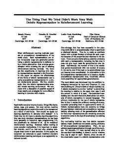
4.2 Policy-based Proto-value Functions As discussed in Section 3, the basic assumption underlying the PVF framework is that the optimal value function V ∗ can be represented on the graph G obtained through a random walk following a policy π R on the environment at hand. Since the optimal value function is defined according to both the transition model T and the reward function R (see Figure 1), the graph should effectively capture both these elements. This requirement is particularly important under the transfer perspective introduced in the previous section. PVFs extracted on the basis of a graph obtained by a random exploration of the environment (from now on denoted as domain-based PVFs) can be effectively used only to achieve domain transfer across tasks. In fact, in this case the implicit assumption is that all the optimal value functions of the tasks can be well approximated by the basis of the domain-based graph, i.e. the graph that captures the dynamics of the environment but completely ignores the reward functions. On the other hand, since in the more general case both the transition model and the reward function can vary from one task to another, the PVFs should be extracted taking into account both of them. Unfortunately, it is not possible to explicitly use the reward function in the construction of the graph. Nonetheless,

Figure 4: An example of averaged graph it is possible to bias the exploration of the environment towards the optimal policy of the source task at hand, thus indirectly taking its reward function into account. This yields to a new sampling policy which is different from the random policy π σ 6= π R . As a result, we can compute a new kind of graph that takes the new sampling policy. Such graph will be denoted as policy-based graph. We now explain how to build policy-based graphs. Consider a task with a completely connected but stochastic domain consisting of 5 states and with the goal in the state in the center, denoted with a cross. A domain-based graph would be the one depicted in Figure 2, where the number on the arcs represent the weights for the (in this case undirected) edges. On the other hand, a policy-based graph should take the goal into account. If the weight matrix of the graph is a stochastic matrix (i.e. it contains probabilities), we can compute its t-th power to obtain the probability distribution after t steps. If this is not performed, then the contribution of the policy is only local and will not produce very different PVFs if compared to domain-based graphs. After this step, we obtain the graph depicted in Figure 3. This graph captures information about the goal, since the weights on the edges directed towards the goal is very high and the other weights are close to 0. However the information about the domain is completely lost. Hence we introduce averaged graph construction methods. For this example, an average graph is the one depicted in Figure 4. This new graph includes information about both the goal and the domain. In particular, weights on edges going towards the goal have a higher value, whereas the other weights correspond to a smaller value but still greater than 0, to preserve domain topology’s information. Following these observations, we propose the state-action graph construction method reported in Algorithm 2. The algorithm takes an δ parameter as input. This parameter is called policy bias factor and it is used to adjust the bias

towards the optimal policy π ∗ in the construction of the graph. In particular we set the sampling policy π σ to:  R π with probability 1 − δ πσ = π∗ with probability δ When δ = 0, a completely exploratory behavior is followed, i.e. the policy is not used at all to construct the graph and both graph and PVFs are extracted from the environment only. On the other hand, when δ is close to 1, then the policy contribution is very strong and the walk (and hence the graph) is strongly leaned towards the goal. In Step 6 the graph averaging is done. One way to average the graph is to use the time-averaged transition probability matrix [4]: Wte =

t 1X i W , t i=1

that stores the probability of being in one state (state-action pair) after starting from some other state (state-action pair) after taking an arbitrary number of steps between 1 and t. Another averaging method produces a discounted graph. This method is more consistent with the RL paradigm. More precisely, given a discount factor γ, the new graph is computed as: t X W i (1 − γ)γ i−1 Wte = . 1 − γt i=1

w(u, v) =

′

′

u = (s, a), v = (s , a ).

This produces a weighted on-policy state-action graph. The weight associated to the edge between (s, a) and (s′ , a′ ) is greater if we want the impact of the policy to be more consistent and smaller otherwise. The amount of biasing towards the policy is controlled by the δ parameter.

5.

//E : //N : //t : //δ :

Number of episodes Number of steps per episode Exponent for the average matrix Policy bias factor

1: Perform a random walk of E episodes, each of maximum N steps, and collect samples in the form hs, a, r, s′ i in the sample set SS. 2: Construct the transition model T and the reward function R from SS 3: Use dynamic programming to compute the optimal policy π ∗ using T and R 4: Use the δ parameter to produce the sampling policy π σ from π (with probability 1 − δ we explore, i.e. we use a random policy, and with probability δ we use π ∗ ). a σ σ 5: Given Tss ′ and π , where π (a, s) is the probability of execution of action a in state s according to π σ , compute the initial weight matrix for the state-action graph by setting each entry to W ((si , ak ), (sj , al )) = Tsai ksj π σ (al |sj ), ∀si , sj ∈ S, ak , al ∈ A 6: Compute the weight matrix of the average graph as Wte =

In step 7 the graph is symmetrized. This is needed in most of the situations, especially when using the Laplacian as defined on undirected graphs, since the estimated transition matrix and in particular the final graph matrix is not symmetric. To produce state-action graphs, we used a modified version of the approach in [?]. The topology of the graph is constructed in the same way as the off-policy approach, however the weighting technique is different. More precisely, a weight associated to the edge is computed as: a σ ′ ′ Tss ′ π (s , a ),

Algorithm 2 BuildGammaSAByPolicy(E ,N ,t,δ)

EXPERIMENTAL RESULTS

In order to compare the learning performance (i.e. the average reward per trial) of domain-based and policy-based PVFs in transfer problem, we consider the three-rooms gridworld domain (Figure 5) used in [14]. This consists in a stochastic environment, where each action is successful with probability 0.9, whereas with probability 0.1 the agent remains in the same state. In Table 1 we enlist the parameters common to all experiments.

5.1 Goal Transfer Experiment We first perform goal transfer experiments. These experiments consider tasks related in terms of their domain but with different reward functions. We extract a total of 24 state-action domain-based PVFs. We would expect domainbased PVFs to perform well, since they effectively capture

or as Wte =

t 1X i W t i=1

t X W i (1 − γ)γ i−1 1 − γt i=1

7: Symmetrize the graph Wte ← WteWte′ , where Wte′ is the transpose of Wte

Table 1: Experiments Common Parameters Type of graph Number of samples Discount factor Max iterations for LSPI ǫ parameter for LSPI

discounted state-action graph 15000 0.9 16 0.001

the representation of the domain. In the first experiment we consider one source task with the goal in the upper right angle of the gridworld, and one target task with the goal in the upper left corner. The value function for the source task is reported in Figure 6. As we can see, it presents some nonlinearities in the regions that are close to the walls. In [14] they already showed that domain-based PVFs can effectively capture those nonlinearities. Learning performance are reported in Figure 7. In this case the two tasks are completely unrelated in terms of their goal and their optimal policy, whereas their domain is the same. Results show that domain-based PVFs can effectively achieve goal transfer in this case. According to the definition of transfer in Section 4.1, we now consider a goal transfer problem in which the reward functions are obtained by perturbation of the reward function of a source task. In the source task the goal is placed at (8, 27), close to the upper-right corner and the correspond-

Learning Performances with domain−based PVFs on Symmetric Goal Transfer 0.08 0.07

Learning performance

0.06 0.05 0.04 0.03 0.02 0.01

Performance with domain−based PVFs Optimal performances

0

1

2

3

4 5 LSPI iteration

6

7

8

Figure 7: Learning performance in goal transfer obtained by moving the goal in a symmetric position

Figure 5: The three-rooms gridworld

Exact Value Function

Exact Value Function

8

10 8

6 6

4

4 2

2

0 15 30

10 20 5

0 15 30

10

10 0

0

20 5

10 0

Figure 6: A value function with nonlinearities generated the transition model. ing optimal value function is reported in Figure 8. It is interesting to notice that, in this case, the value function has many nonlinearities that are not related to the topology of the environment but that are generated by the reward function. Thus, the domain-based PVFs are likely to fail to approximate the optimal value functions of target tasks that share these characteristics with the source task. On the other hand, the policy-based PVFs generated from the graph obtained by biasing the exploration towards the optimal policy of the source task, better capture the particular shape of the value functions to approximate. Also in this experiment we extract 24 state-action PVFs. We consider 9 target tasks where the goal is moved around the goal of the source task (including itself). We plot the average learning performances of domain-based PVFs and policy-based PVFs obtained with policy bias factor set to 0.75, and we compare them with the average optimal performance. Results are reported in Figure 9. As it can be noticed, policy-based PVFs performs better than domain-based PVFs. The tasks we are considering in this experiment are related both in terms of their domain and in terms of the optimal policy. The value function to be approximated contains a nonlinearity close to the goal that cannot be captured by domain-based PVFs. Furthermore, we see how policy-based PVFs can help to capture and transfer the information about the nonlinearities close to the goal, thanks to the fact that we are

0

Figure 8: A value function with nonlinearities generated by the reward function and not the transition model. also transferring information about the optimal policy of the source task which shares some commonalities with those of the target tasks.

5.2 Domain Transfer Experiment Next, we consider a domain transfer experiment. In this experiment we consider tasks that are strictly related in terms of their optimal policy but with different underlying domains. Hence we also assume that their shared representation can be compactly extracted by using a low number of PVFs. In this experiment we consider only 6 PVFs, as we assume the representation to be captured can be compacted in a few number of PVFs. The source task has a domain which is “tilted” in the opposite direction of the goal. This means that the probability of success of actions that aims in the opposite direction of the goal are higher than the one aiming towards the goal. In the target task, the domain is the standard “untilted” one, with actions having the same probability of success. The goal is placed in the upper-right corner in both tasks. Figure 10 compares the learning performance of domain-based PVFs with those of policy-based PVFs obtained with policy bias factor set to 0.75. Optimal performances are reported as well. As we can see, policybased PVFs outperform domain-based PVFs in this transfer

Learning Performance comparing domain−based PVFs with policy−based PVFs in goal transfer in multiple target tasks

Learning performance comparing domain−based PVFs with policy−based PVFs in goal and domain transfer 0.1

0.1 0.09

Performance with domain−based PVFs

0.09

Performance with Policy−based PVFs

Performance with domain−based PVFs

0.07 0.06 0.05 0.04

Optimal performance

0.06 0.05 0.04

0.02

0.02

0.01

0.01

0

0

2

4

6

8

10 LSPI iteration

12

14

16

18

Figure 9: Learning performance in goal transfer obtained by moving the goal in states around coordinates (8, 27)

0.07 0.06 0.05 0.04 Performance with domain−based PVFs 0.03

Performance with policy−based PVFs Optimal performance

0.02 0.01

1

2

3

4

5 6 LSPI iteration

7

8

2

4

6

8 10 LSPI iteration

12

14

16

Figure 11: Learning performance in goal and domain transfer

6. CONCLUSIONS

Learning performance comparing domain−based PVFs with policy−based PVFs in domain transfer 0.08


0.07

0.03

0.03

0

Performance with policy−based PVFs

0.08

Average optimal performance



0.08

9

10

Figure 10: Learning performance in domain transfer

experiment. This is because the two tasks share the representation about their optimal policy, and this can be easily captured using policy-based PVFs, whereas domain-based PVFs are not able to extract this representation information.

5.3 Goal-Domain Transfer Experiment In the final experiment we consider a case where both the domain and the goal changes. We consider a source task whose domain is tilted towards the bottom-left direction, and a goal set in coordinates (8, 27). We consider three target tasks: the first has a standard untilted domain and the goal set in coordinates (8, 28); the second has the domain tilted towards north and the goal set in coordinates (9, 27); the third has the domain tilted towards south and the goal set in coordinates (9, 26). Also in this experiment we consider 6 PVFs for the same reason as the previous experiment, by setting the policy bias factor to 0.5. Figure 11 compares the learning performance of domain-based PVFs with those of policy-based PVFs. Optimal performances are reported as well. Also in this case, policy-based PVFs outperform domain-based PVFs. By transferring information about the optimal policy, we are able both to counter-balance the effect of the nonlinearity close to the goal and the change in the domain.

In this paper we focused on the problem of transfer in terms of the extraction of a set of basis functions that can be profitably used for the approximation of the optimal value functions of a set of related tasks. In particular, building on the PVF framework, we showed that, in the transfer problem, the graph construction method should take into consideration both the transition model and the reward function. Hence, we proposed the use of an averaged discounted graph obtained through a biased exploration of the environment. Thus, the graph successfully captures the representation shared across different tasks, and the corresponding policy-based PVFs are likely to effectively approximate the optimal value functions of the target tasks. The experimental activity, although preliminary, showed that the policy-based PVFs perform better than domain-based PVFs in goal and domain transfer problems and also when both the goal and the domain are varied from the source to the target tasks. In particular, in the case of goal transfer, domain-based PVFs are able to provide effective transfer whenever the optimal value functions has nonlinearities directly related with the intrinsic structure of the environment. On the other hand, when optimal value functions present some nonlinearities caused by the reward function, the use of the optimal policy of the source target leads to the extraction of policy-based PVFs that can better approximate the target functions. Furthermore, the experiments of domain transfer experiments showed that the policy-based PVFs can improve the transfer capabilities in cases where the source and the target task share a similar optimal policy, but the domains are different. Finally, we analyzed experiments of goal-domain transfer, in which the policy-based PVFs confirmed a performance improvement with respect to the domain-based PVFs. One major drawback of policy-based PVFs is their computational complexity. The construction of the state-action graph becomes rapidly infeasible in complex problems. Furthermore, PVFs are stored in a tabular form, i.e., each PVF is a vector of size |S| × |A|, but this has often the same complexity of storing in a tabular form the optimal value function itself. Hence, there is the need to devise techniques able to introduce a parametrization of PVFs that allows to derive PVFs with a limited set of parameters. Another direction for future work is the improvement of

the PVFs for transfer problems. In this paper, we considered the scenario in which the PVFs are extracted from one source task and then reused in a series of target tasks. On the other hand, it would be possible to define a method to incrementally adapt the initial set of PVFs according to the target tasks at hand, thus improving their approximation capabilities on the tasks that must be actually solved. Finally, the extraction of PVFs could be extended, under a multi-task perspective, to the problem of the extraction of a set of basis functions that effectively capture the underlying structure common to the optimal value functions of a set of tasks [1].

7.

REFERENCES

[1] A. Argyriou, C. A. Micchelli, M. Pontil, and Y. Ying. A spectral regularization framework for multi-task structure learning. In NIPS, 2007. [2] B. Banarjee and P. Stone. General game learning using knowledge transfer. In Proceedings of the 20th International Joint Conference on Artificial Intelligence, 2007. [3] A. G. Barto, S. Singh, and N. Chentanez. Intrinsically motivated learning of hierarchical collections of skills. In Proceedings of the 3rd International Conference on Development and Learning (ICDL 2004), 2004. [4] A. T. Bharucha-Reid. Elements of the Theory of Markov Processes and Their Applications. Dover Publications, 1997. [5] A. Bonarini, A. Lazaric, and M. Restelli. Incremental skill acquisition for self-motivated learning animats. In From Animals to Animats 9 (SAB), 2006. [6] F. R. Chung. Spectral Graph Theory. Amer Mathematical Society, 1997. [7] T. G. Dietterich. Hierarchical reinforcement learning with the MAXQ value function decomposition. Journal of Artificial Intelligence Research, 13:227–303, 2000. [8] B. Falkenhainer, K. D. Forbus, and D. Gentner. The structure-mapping engine: Algorithm and examples. Artificial Intelligence, 41(1):1–63, 1989. [9] K. Ferguson and S. Mahadevan. Proto-transfer learning in markov decision processes using spectral methods. In ICML Workshop on Transfer Learning, 2006. [10] G. Konidaris and A. Barto. Autonomous shaping: Knowledge transfer in reinforcement learning. In Proceedings of the 23rd International Conference on Machine Learning, 2006. [11] G. Konidaris and A. Barto. Building portable options: Skill transfer in reinforcement learning. Technical report, University of Massachusetts, Department of Computer Science, 2006. [12] M. G. Lagoudakis and R. Parr. Least-squares policy iteration. JMLR, 4:1107–1149, 2003. [13] Y. Liu and P. Stone. Value-function-based transfer for reinforcement learning using structure mapping. In Proceedings of the Twenty-First National Conference on Artificial Intelligence, pages 415–20, July 2006. [14] S. Mahadevan and M. Maggioni. Proto-value functions: A laplacian framework for learning representation and control in markov decision processes. JMLR, 8:2169–2231, 2007.

[15] A. McGovern and A. G. Barto. Automatic discovery of subgoals in reiforcement learning using diverse density. In 18th International Conference on Machine Learning, 2001. [16] N. Mehta, S. Natarajan, P. Tadepalli, and A. Fern. Transfer in variable-reward hierarchical reinforcement learning. In NIPS 2005 Workshop, Inductive Transfer: 10 Years Later, 2005. [17] I. Menache, S. Mannor, and N. Shimkin. Q-cut dinamic discovery o sub-goals in reinforcement learning. In Thirteenth European Conference on Machine Learning, 2002. [18] M. Petrik. An analysis of laplacian methods for value function approximation in mdps. In IJCAI, pages 2574–2579, 2007. [19] A. A. Sherstov and P. Stone. Improving action selection in mdps via knowledge transfer. In Proceedings of the Twentieth National Conference on Artificial Intelligence, 2005. [20] D. Silver, G. Bakir, K. Bennett, R. Caruana, M. Pontil, S. Russell, and P. Tadepalli, editors. Workshop on ”Inductive Transfer : 10 Years Later” at NIPS, 2005. ¨ Simsek and A. G. Barto. Using relative novelty to [21] O. identify useful temporal abstractions in reinforcement learning. In ICML, 2004. [22] R. S. Sutton and A. G. Barto. Reinforcement Learning: An Introduction. MIT Press, Cambridge, MA, 1998. [23] M. E. Taylor, P. Stone, and Y. Liu. Value functions for RL-based behavior transfer: A comparative study. In AAAI, pages 880–885, July 2005. [24] M. E. Taylor, P. Stone, and Y. Liu. Transfer learning via inter-task mappings for temporal difference learning. JMLR, 8:2125–2167, 2007. [25] M. E. Taylor, S. Whiteson, and P. Stone. Transfer via inter-task mappings in policy search reinforcement learning. In Autonomous Agents and Multi-Agent Systems Conference, 2007. [26] T. J. Walsh, L. Li, and M. L. Littman. Transferring state abstractions between mdps. In ICML-06 Workshop on Structural Knowledge Transfer for Machine Learning, 2006.